Scalable Coupling of Deep Learning with Logical Reasoning

Abstract

In the ongoing quest for hybridizing discrete reasoning with neural nets, there is an increasing interest in neural architectures that can learn how to solve discrete reasoning or optimization problems from natural inputs. In this paper, we introduce a scalable neural architecture and loss function dedicated to learning the constraints and criteria of NP-hard reasoning problems expressed as discrete Graphical Models. Our loss function solves one of the main limitations of Besag’s pseudo-loglikelihood, enabling learning of high energies. We empirically show it is able to efficiently learn how to solve NP-hard reasoning problems from natural inputs as the symbolic, visual or many-solutions Sudoku problems as well as the energy optimization formulation of the protein design problem, providing data efficiency, interpretability, and a posteriori control over predictions.

1 Introduction

In recent years, several hybrid neural architectures have been proposed to integrate discrete reasoning or optimization within neural networks. Many of the architectures incorporate an optimization or reasoning layer in a neural network where the previous layer outputs the parameters defining the criteria of the discrete problem Wang et al. (2019); Amos and Kolter (2017); Mandi and Guns (2020); Pogančić et al. (2020); Mandi et al. (2022); Sahoo et al. (2023). Learning is then achieved by back-propagating gradients from known solutions and natural inputs (such as symbols, images, text or molecule geometries). In this paper, we are more specifically interested in scalable learning when the underlying discrete reasoning problem incorporates unknown logical (deterministic) information or constraints.

Our contributions are twofold: we introduce a hybrid architecture combining arbitrary deep learning layers with a final discrete NP-hard Graphical Model (GM) reasoning layer and propose a new loss function that efficiently deals with logical information. We use discrete GMs Cooper et al. (2020) as the reasoning language because GMs have been used to represent both Boolean functions (in propositional logic, constraint networks) and constrained numerical functions (partial weighted MaxSAT, Cost Function Networks). Also, a probabilistic interpretation of such models is available in stochastic GMs such as Markov Random Fields (MRFs), where infinite costs represent zero probabilities (infeasibility).

Besides the discrete nature of variables that defines zero gradients almost everywhere, the Boolean nature of logic creates an additional challenge. Indeed, constraints are either satisfied or violated and the continuous relaxation of Boolean satisfiability or constraint satisfaction in weighted variants Wang et al. (2019); Brouard et al. (2020); Palm et al. (2018) may not always account for the potentially redundant nature of constraints: in some contexts, a meaningful constraint $c$ may be implied by a set of other constraints $C$, making the learning of $c$ from examples impossible if $C$ has already been learned.

In our architecture, during inference, an arbitrary deep learning architecture receives natural inputs and outputs a fully parameterized discrete GM. This GM can then be solved using any suitable optimization solver. To benefit from the guarantees of logical reasoning on proper input, we use the exact GM prover toulbar2 Allouche et al. (2015). During learning, GMs computed from natural inputs need to be gradually improved from solutions in the data set. Given the NP-hard nature of discrete GM reasoning and our target of scalable learning, using an exact optimization during learning seems inadequate: even if the finally predicted GMs may be empirically easy to solve (as is the case, e.g., for the Sudoku problem), the GMs predicted in the early epochs of learning are essentially random, defining empirically extremely hard instances that cannot be solved to optimality in a reasonable time Zhang (2001). Relying instead on more scalable convex relaxations of the discrete GM optimization problem Durante et al. (2022) would come at the cost of sacrificing the guarantees of logical reasoning on proper input.

We instead exploit the probabilistic interpretation of weighted GMs and target the optimization of the asymptotically consistent and scalable Negative Pseudo-LogLikelihood (NPLL) of the training data set Besag (1975). However, this loss function is plagued with an incapability of dealing with large costs Montanari and Pereira (2009) and therefore with constraints. In this paper, we analyze the reasons for this incapability and show that it can be explained by the context-dependent redundancy of logical information. We propose a variant, the E-NPLL, for scalable decision-focused learning. With this differentiable informative loss, our architecture is able to efficiently learn from natural inputs to, e.g., solve the Visual Sudoku Wang et al. (2019); Brouard et al. (2020). We also apply it to a many-solutions Sudoku data set Nandwani et al. (2021) and to a data set of Protein Design instances including several hundreds of variables. With an exact prover used during inference, 100% accuracy can be reached on the symbolic Sudoku, even with small data sets. Moreover, the output of the penultimate layer being a full GM, it can be scrutinized to detect possible symmetries Lim et al. (2022) for example. It is also possible to introduce a posteriori constraints to get solutions that satisfy desirable properties or even bias the learned criteria by adding new functions to the produced GM.

2 Preliminaries

2.1 Background

A discrete graphical model is a concise description of a joint function of many discrete variables as the combination of many simple functions. Depending on the nature of the output of the functions (Boolean or numerical), and how they are combined and described, GMs cover a large spectrum of AI NP-hard reasoning and optimization frameworks including Constraint Networks, Propositional Logic as well as their numerical additive variants Cost Function Networks and partial weighted MaxSAT Cooper et al. (2020). Following cost exponentiation and normalization, these numerical joint functions can describe joint probability distributions, as done in Markov Random Fields (MRFs). In this paper, we use Cost Function Networks for their ability to express both numerical and logical functions. We assume here that cost functions take their value in $\bar{\mathbb{R}}=\mathbb{R}\cup\{\infty\}$.

In the rest of the document, we denote sequences, vectors, tensors in bold. Variables are denoted in capitals with a given variable $Y_{i}\in\mathbf{Y}$ being the $i^{th}$ variable in the sequence $\mathbf{Y}$. An assignment of the variables in $\mathbf{Y}$ is denoted $\mathbf{y}$ and $y_{i}$ is the assignment of $Y_{i}$ in $\mathbf{y}$. $\mathbf{Y}_{-i}$ denotes the sequence of variables $\mathbf{Y}$ after removal of variable $Y_{i}$ and similarly for $\mathbf{y}_{-i}$ given $\mathbf{y}$. For a set of variables $\mathbf{M}\subset\mathbf{Y}$, we also note $\mathbf{Y}_{-M}=\mathbf{Y}\setminus\mathbf{M}$ and $\mathbf{y}_{-M}$ their values in $\mathbf{y}$. The domain of a variable $Y_{i}$ is a set denoted $D^{i}$ with $|D^{i}|\leq d$, the maximum domain size. For a sequence of variables $\mathbf{Y}$ we denote as $D^{\mathbf{Y}}$ the Cartesian product of all $D^{i}$ with $Y_{i}\in\mathbf{Y}$. A cost function over a subset of $\mathbf{Y}$ described by a tensor (cost matrix) over $\bar{\mathbb{R}}$ is called an elementary cost function.

Definition 1.

Given a sequence $\mathbf{Y}=\{Y_{1},\ldots,Y_{n}\}$ of $n$ finite domain variables, a cost function network $C$ is defined as a set of elementary cost functions. It defines a joint cost function, also denoted $C(\cdot)=\sum_{F\in C}F$, involving all variables in $\mathbf{Y}$. The optimization problem, known as the Weighted Constraint Satisfaction Problem (WCSP), is to find an assignment $\mathbf{y}$ that minimizes the joint function $C(\mathbf{y})$. If $C(\mathbf{y})<\infty$, $\mathbf{y}$ is called a solution (a model in propositional logic).

In stochastic GMs such as MRFs, the joint function $C(\cdot)$ is used to define a joint probability distribution $P^{C}~{}\propto~{}exp(-C(\cdot))=\prod_{F\in C}exp(-F)$ requiring the expensive computation of a #-P-hard normalizing constant.

When a given function $F$ is never larger than another function $F^{\prime}(F\leq F^{\prime})$, $F$ is known as a relaxation of $F^{\prime}$. A constraint is a cost function $F$ such that $F(\mathbf{t})\in\{0,\infty\}$: it exactly forbids all assignments $\mathbf{t}$ such that $F(\mathbf{t})=\infty$. When $F\leq F^{\prime}$ are constraints, we say that $F$ is a logical consequence of $F^{\prime}$: whenever $F^{\prime}$ is satisfied (equal to $0$), $F$ is satisfied too. For a set of constraints $C$, $F\in C$ is redundant w.r.t. $C$ iff $C$ and $C\setminus\{F\}$ define the same function. At a finer grain, we say $F$ is partially redundant if $\exists F^{\prime}<F$ such that $(C\setminus\{F\})\cup\{F^{\prime}\}$ and $C$ define the same function. Consider for example $\mathbf{Y}=\{Y_{1},Y_{2},Y_{3},Y_{4}\}$ with domains $\{0,1\}$ and $C=\{Y_{1}\neq Y_{2},Y_{2}+Y_{3}>1,Y_{3}\neq Y_{4}\}$. No constraint is redundant in $C$, but in the context of the assignment $\{Y_{2}=1,Y_{3}=1\}$, the constraint $Y_{2}+Y_{3}>1$ becomes redundant w.r.t. $C^{\prime}=C\cup\{Y_{2}=1,Y_{3}=1\}$ . In the context of $\{Y_{1}=0\}$, $Y_{2}+Y_{3}>1$ becomes partially redundant, as it could equivalently be replaced by the weaker $Y_{2}=Y_{3}$. Because of redundancies, the observed values in a sample can create a context that makes some constraints redundant and therefore not learnable.

For $n$ variables, a strictly pairwise graphical model $C$ ($\forall F\in C$, $F$ involves exactly $2$ variables) can be described with $n(n-1)/2$ elementary cost function with tensors (matrices) of size at most $d^{2}$. We denote by $C[i,j]$ the tensor describing the cost function $F_{ij}$ between variables $Y_{i}$ and $Y_{j}$. Thus $F_{ij}(Y_{i}=a,Y_{j}=b)$ is simply $C[i,j](a,b)$.

2.2 Problem Statement

In this work, we assume that we observe samples $(\omega,\mathbf{y})$ of the values $\mathbf{y}$ of the variables $\mathbf{Y}$ as low-cost solutions of an underlying constrained optimization problem with parameters influenced by natural inputs $\omega$. From a data set $S$ of pairs $(\omega,\mathbf{y})$, we want to learn a model $N$ (in our case, a neural network) which predicts a pairwise graphical model $N(\omega)$ such that $\mathbf{y}\in\operatorname*{\arg\!\min}_{\mathbf{y}\in D^{\mathbf{Y}}}N(\omega)(\mathbf{y})$. Such a graphical model $C=N(\omega)$ defines the last layer of our hybrid neural+graphical model architecture (see Figure 1).

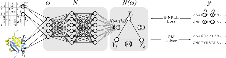
Figure 1: Our hybrid learning architecture: natural inputs $\omega$ (left) feed a neural net $N$ in charge of predicting all pairwise cost functions $F_{ij}$ of the GM $N(\omega)$. To learn $N$, we back-propagate solutions $\mathbf{y}\in S$ through the E-NPLL loss function. At inference, $N(\omega)$ can be directly fed to any GM solver, be it exact, based on a scalable relaxation or a (meta)-heuristics. This is illustrated here on 2 possible problems: a visual Sudoku problem (top) and a protein design problem (bottom).

In terms of supervision, we assume that the variables in $\mathbf{Y}$ are identified but we also want to exploit any information that would be available on elements of $\omega$. Some of these natural inputs may be direct constraints or assignments of variables in $\mathbf{Y}$ that can be directly incorporated into the GM $N(\omega)$, others may be known to influence only a subset of all the variables $\mathbf{Y}$. In the symbolic Sudoku problem, a partially filled grid of numbers is observed in $\omega$ and each observed value in the grid is known to be the value of its corresponding variable. Similarly, in the visual Sudoku, each image of a digit in the grid is known to represent the value of a single variable, observed in $\mathbf{y}$, providing grounding information Chang et al. (2020).

Assuming the data set $S$ contains i.i.d. samples from an unknown probability distribution $P(\mathbf{Y}|\omega)$, a natural loss function for the GM $N(\omega)$ is the asymptotically consistent negative logarithm of the probability $\textrm{NLL}(S)=-\log(\prod_{(\omega,\mathbf{y})\in S}P^{N(\omega)}(\mathbf{Y}=\mathbf{y}))$ of the observed samples. This negative loglikelihood is however intractable because of the #P-hard normalizing constant. We instead rely on the asymptotically consistent tractable negative pseudo-loglikelihood Besag (1975) $\textrm{NPLL}(S)=\sum_{(\omega,y)\in S}-\log(\prod_{i}P^{N(\omega)}(y_{i}|\mathbf{y}_{-i}))$. The NPLL works at the level of each variable $Y_{i}$, in the context of $\mathbf{y}_{-i}$, the assignment of all other variables. It requires only normalization over one variable $Y_{i}$, a computationally easy task.

Property 1.

For $Y_{i}$, we have $P(Y_{i}|\mathbf{y}_{-i})=\mathrm{softmax}(-m_{i}(Y_{i}))$ where $m_{i}(Y_{i})=\sum_{j\neq i}F_{ij}(Y_{i},y_{j})$. In a message passing interpretation, $m_{i}(\cdot)\in\bar{\mathbb{R}}^{|D^{i}|}$ represents the sum of all messages received from neighbor variables $Y_{j}$ through the incident functions $F_{ij}$, given $Y_{j}=y_{j}$. Computing the NPLL is in $O(n(n-1)d)$ per sample and epoch. It can easily be vectorized (computed independently on each variable).

The NPLL enables scalable training from natural inputs assuming an underlying GM NP-hard optimization problem. However, the proof of asymptotic consistency of the NPLL Besag (1975); Geman and Graffigne (1986) relies on identifiability assumptions that obviously do not hold in the context of constraints (zero probabilities) because of redundant constraints. Unsurprisingly, the NPLL is known to perform poorly in the presence of large costs Montanari and Pereira (2009). Empirically, we observed that the resulting architecture completely fails at solving even the simplest symbolic Sudoku problem where $\omega$ contains the digits from the unsolved Sudoku grid and $\mathbf{y}$ is the corresponding solution.

3 The E-NPLL

To understand the incapacity of the NPLL to deal with large costs, it is interesting to look into the contribution of every pair $(\omega,\mathbf{y})$ to the gradient $\frac{\partial NPLL}{\partial N(\omega)[i,j](v_{i},v_{j})}$ of the NPLL for a given pair of values $(v_{i},v_{j})$ of a pair of variables $(Y_{i},Y_{j})$.

Property 2 (see full paper).

The contribution of a pair $(\omega,\mathbf{y})$ to the gradient $\frac{\partial NPLL}{\partial N(\omega)[i,j](v_{i},v_{j})}$ is equal to

$$[\mathbb{1}(y_{i}=v_{i},y_{j}=v_{j})-P^{N(\omega)}(v_{i}|\mathbf{y}_{-i})\mathbb{1}(y_{j}=v_{j})]\\ +[\mathbb{1}(y_{i}=v_{i},y_{j}=v_{j})-P^{N(\omega)}(v_{j}|\mathbf{y}_{-j})\mathbb{1}(y_{i}=v_{i})]$$

The two terms in the gradient above come from NPLL terms computed on variables $Y_{i}$ and $Y_{j}$ respectively. Consider our previous example with four variables, $C=\{Y_{1}\neq Y_{2},Y_{2}+Y_{3}>1,Y_{3}\neq Y_{4}\}$ and $\mathbf{y}=(0,1,1,0)$. We focus on the variables $Y_{i=2}$ and $Y_{j=3}$ and assume that $C$ should hold under $\omega$, which means that the pair of values $(Y_{2}=0,Y_{3}=0)$ should be predicted as forbidden. Being forbidden under $\omega$, $\mathbb{1}(y_{2}=0,y_{3}=0)=0$. If additionally, the forbidden pairs $(Y_{1}=0,Y_{2}=0)$ and $(Y_{3}=0,Y_{4}=0)$ have already reached a high cost under $\omega$, then both $P^{N(\omega)}(Y_{2}=0|\mathbf{y}_{-2})$ and $P^{N(\omega)}(Y_{3}=0|\mathbf{y}_{-3})$ will be close to zero, as well as the gradient itself. This will lead to a negligible (if any) change in the cost of the pair $(Y_{2}=0,Y_{3}=0)$: learning will be blocked or tremendously slowed down. Said otherwise, the fact that, in the context of $(\omega,\mathbf{y})$, the forbidden pair $(Y_{2}=0,Y_{3}=0)$ is redundant w.r.t. already identified forbidden pairs $(Y_{1}=0,Y_{2}=0)$ and $(Y_{3}=0,Y_{4}=0)$ effectively prevents any change in the cost $N(\omega)[2,3](0,0)$. The issue with the NPLL lies therefore in the dynamic of the stochastic gradient optimization: the early identification of some high costs under $\omega$ will prevent the increase of other significant costs which are redundant in the context of the observed $\mathbf{y}$, but not redundant in the unconditioned problem.

Inspired by “dropout” in deep learning Srivastava et al. (2014), we introduce the Emmental NPLL (E-NPLL) as an alternative to the NPLL that should still work when constraints (infeasibilities) are present in $S$.

Definition 2.

The E-NPLL is a stochastic loss defined as $\textrm{E-NPLL}(\mathbf{y})=-\sum_{Y_{i}\in\mathbf{Y}}\log(P^{N(\omega)}(y_{i}|\mathbf{y}_{-(\{i\}\cup\mathbf{M}_{i})}))$ where each $\mathbf{M}_{i}$ is a random subset of $\{1,\ldots,n\}\setminus\{i\}$.

In the above formula, $P^{N(\omega)}(y_{i}|\mathbf{y}_{-(\{i\}\cup\mathbf{M}_{i})})$ is a short (and slighly abusive) notation for $\mathrm{softmax}(-m_{i}(Y_{i}))$ where $m_{i}(Y_{i})=\sum_{j\not\in\{i\}\cup\mathbf{M}_{i}}F_{ij}(Y_{i},y_{j})$. The idea of the E-NPLL follows directly from the previous gradient analysis: to prevent a combination of incident functions with already-learned high cost from shrinking gradients, we mute a random fraction of the incident functions. This is used in combination with an L1 regularization on the output of the learned network $N(\omega)$ to favour the prediction of exact zero costs which makes the GM optimization problem easier to solve. Because the E-NPLL is designed to fight the side effects of redundant constraints on gradients, we expect it to learn a GM $N(\omega)$ with all redundant pairwise constraints.

3.1 Redundancy and Many Solutions

We hypothesize that existing neural architectures where an exact solver is called during training will instead be insensitive to redundant constraints and will tend to not predict them. Contrarily to the NPLL that analyzes $N(\omega)$ independently for every variable $Y_{i}$ in the context of $\mathbf{y}_{-i}$, a solver will deal with the global problem and the presence or absence of globally redundant constraints will not affect its output and therefore the associated loss. With L1 regularization, we hypothesize that redundant constraints will tend to disappear. We will test this using the Hinge loss Tsochantaridis et al. (2005), a well-known differentiable upper bound of the Hamming distance between a solver solution $\operatorname*{\arg\!\min}_{\mathbf{y}\in D^{\mathbf{Y}}}N(\omega)(\mathbf{y})$ and the observed $\mathbf{y}$. Note that in our settings, the Hinge loss is equivalent (under conditions detailed in the full paper) to the recent loss of Sahoo et al. (2023).

When a solver is called during training on $(\omega,\mathbf{y})$, the output of the solver is compared to the solution $\mathbf{y}$. But reasoning problems usually have more than one solution and non-zero gradients get back-propagated when the predicted solution is different from the observed one, even if it is a correct one. It has been argued that this can severely hamper the training ability of solver-based layers, and Reinforcement Learning strategies have been defined to fight this Nandwani et al. (2021). Because it does not rely on the comparison of an arbitrary solver solution of the underlying discrete problem with the solution $\mathbf{y}$ in the data set, our approach should be directly able to deal with problems with many solutions.

4 Related Works

As Palm et al. (2018); Wang et al. (2019); Amos and Kolter (2017); Brouard et al. (2020); Pogančić et al. (2020); Sahoo et al. (2023), we assume we have a data set of pairs $(\omega,\mathbf{y})$ where $\mathbf{y}$ is sampled from a distribution of feasible high-quality solutions of a discrete reasoning problems whose parameters are influenced by $\omega$. We want to be able to predict solutions for new values of $\omega$. While Brouard et al. (2020) proposed a non-differentiable architecture, most recent proposals, including ours, provide a differentiable DL architecture that enables learning from observables $\omega$ including natural inputs. All architectures exploit an optimization model with continuous parameters that are predicted by the previous layer. For training, a discrete differentiable reasoning layer can be used, requiring one Tsochantaridis et al. (2005); Sahoo et al. (2023); Berthet et al. (2020); Niepert et al. (2021) or two Pogančić et al. (2020) solver calls per training sample at each epoch. On NP-hard problems, such as MaxSAT or integer linear programming, these architectures may have excruciating training costs and are therefore applied only on tiny instances ($20$-cities traveling salesperson problems Pogančić et al. (2020) or 3 jobs/10 machines scheduling problems Mandi et al. (2022)). For more scalability, relaxations of the underlying NP-hard problem using continuous optimization Amos and Kolter (2017); Wang et al. (2019); Mandi and Guns (2020); Wilder et al. (2019) or lifted message passing Palm et al. (2018) have been used for efficient approximate solving.

For training, the architecture we propose relies instead on a dedicated loss function (that can therefore not be easily changed). At inference, the output of the architecture is a full GM that can be optimized with any suitable optimizer. This implies that our layer is the last layer of the architecture, which is probably a reasonable assumption for most decision-focused learning problems Wilder et al. (2019).

In the Predict-and-optimize framework Elmachtoub and Grigas (2022); Mandi et al. (2020), a known optimization problem needs to be solved but some parameters $\mathbf{v}$ in the criterion must be predicted using historical records of pairs $(\omega,\mathbf{v})$. $\mathbf{v}$ being available at training, the optimization problem can be solved and the regret (the loss in criteria generated by using predicted instead of true values of $\mathbf{v}$) can be computed and used as a loss. In our case, we only have an unlabeled solution $\mathbf{y}$ instead of the optimization parameters $\mathbf{v}$. The reader is referred to the review of Kotary et al. (2021) for more details on end-to-end constrained optimization learning.

Learning constraint is also central in constraint acquisition Bessiere et al. (2017), where guaranteed learning of constraints is achieved using positive/negative examples, in interaction with an agent. We instead assume a fixed data set with just positive examples annotated by features $\omega$, a setting where guarantees are essentially unreachable. Our approach is closer to Beldiceanu and Simonis (2016), where global (instead of elementary) constraints are learned from solutions of highly-structured problems, without differentiability.

5 Experiments

We test our architecture on logical (feasibility) problems with one or many solutions Nandwani et al. (2021), $\omega$ being purely symbolic or containing images. We also apply it to a real, purely data-defined, discrete optimization problem to check the ability of the E-NPLL to estimate a criteria.

Unless specified otherwise, all experiments use a Nvidia RTX-6000 with 24GB of VRAM and a $2.2$ GHz CPU with 128 GB of RAM. Our code is written in Python using PyTorch version 11.10.2 and PyToulbar2 version 0.0.0.2. We use the Adam optimizer with a weight decay of $10^{-4}$ and a learning rate of $10^{-3}$ (other parameters take default values). An L1 regularization with multiplier $2.10^{-4}$ is applied on the cost matrices $N(\omega)[i,j]$. Code and data are available at https://forgemia.inra.fr/marianne.defresne/emmental-pll.

5.1 Learning To Play the Sudoku

The NP-complete Sudoku problem is a classical logical reasoning problem that has been repeatedly used as a benchmark in a “learning to reason” context Palm et al. (2018); Amos and Kolter (2017); Wang et al. (2019); Brouard et al. (2020). The task is to learn how to solve new Sudoku grids from a set of solved grids, without knowing the game rules.

Task.

Given samples $(\omega^{l},\mathbf{y}^{l})$ of initial and solved Sudoku grids, we want to learn how to solve new grids. Sudoku players know that Sudoku grids can be more or less challenging. As one could expect, it is also harder to train how to solve hard grids than easy grids Brouard et al. (2020). We use the number of initially filled cells (hints) as a proxy to the problem hardness, a grid with few hints being hard. The minimal number of hints required to define a single solution is 17, defining the hardest single-solution Sudoku grids. We use an existing data set Palm et al. (2018), composed of single-solution grids with $17$ to $34$ hints. We use $1,000$ grids for training, and $256$ for validation (all hardness). As in Palm et al. (2018), we test on the hardest 17-hints instances, $1,000$ in total.

A $9\times 9$ Sudoku grid is represented as $81$ cell coordinates with a possible hint when available. Each cell is represented by a GM variable with domain $\{1,\ldots,9\}$. For $N$, we use a Multi-Layer Perceptron (MLP) with $10$ hidden layers of $128$ neurons and residual connections He et al. (2016) every $2$ layers. It receives the pairs of coordinates of pairs of cells $(Y_{i},Y_{j})$ and predicts all pairwise cost matrices $N(\omega)[i,j]$. Hints are used to set the values of their corresponding variable in $N(\omega)$. Performances are measured by the percentage of correctly filled grids; no partial credit is given for individual digits.

The resulting architecture learns how to solve the Sudoku and provides rules in $N(\omega)[i,j]$. For pairs of cells on the same row, column or $3$ sub-square, we expect soft difference-like cost function to be predicted (a matrix with a strictly positive diagonal and zeros) that prevents the use of the same value for the two variables. With the L1 regularization on the output of the neural net, other cost matrices should be $0$, indicating the absence of a pairwise constraint.

Grids with a unique solution.

We first train our network with the regular NPLL loss. As expected, it learns only a subset of the rules that suffices to make all other rules redundant: for a cell $Y_{i}$ in the context of $\mathbf{y}_{-i}$, a single clique of difference constraints for every row (or column, or square) is sufficient to determine the value of the cell $Y_{i}$ from $\mathbf{y}_{-i}$, creating vanishing gradients for all other constraints that are instead estimated as constant $0$ matrices. On the test set, inference completely fails.

We replaced the NPLL by the E-NPLL, ignoring messages from $k$ randomly chosen other variables. In terms of accuracy, the training is largely insensitive to the value of the hyper-parameter $k$ (see Table 1) as long as it is neither $0$ (regular NPLL) nor close to $n-1$ (no information). However, larger values of $k$ tend to lead to longer training. We set $k=10$ for all Sudoku experiments. In this case, training takes less than $15$ minutes. At inference, the predicted $N(\omega)$ leads to 100% accuracy on the $1,000$ hard test-set grids.

$k$	Epochs	Training time (s)	Runs with 100% test grids solved
$0$	$100$	-	$0$%
$10$	$23.2\pm 2.6$	$566\pm 67$	$100$%
$20$	$38.6\pm 6.9$	$900\pm 151$	$90$%
$50$	$50.4\pm 7.6$	$1257\pm 184$	$90$%
$70$	$27.2\pm 2.7$	$724\pm 83$	$100$%
$80$	$100$	-	$0$%

Table 1: Average performances over $10$ initialization, for various number of E-NPLL holes $k$. Training is limited to $100$ epochs.

In Table 2, we compare our results with previous approaches that learn how to solve Sudoku. The Graph Neural Net approach of Recurrent Relational Network (RRN) Palm et al. (2018), the convex optimization layer SATNet Wang et al. (2019) and a hybrid ML/CP method Brouard et al. (2020). It should be noted that SATNet’s accuracy is measured on a test set of easy Sudoku grids (avg. 36.2 hints). All the methods that rely on an exact solver are able to reach 100% accuracy but the modeling flexibility of Deep Learning offers the ability to describe the grid geometry in $\omega$, leading to better inductive bias and far better data efficiency. In our case, with $k=10$, we still obtain 100% accuracy on 17-hints grids using a training set of just $200$ grids. More epochs are necessary (less than $200$) but the training time does not increase ($587\pm 32s$ over 10 training using 10 different seeds).

Approach	Acc.	#hints	Train set	Param.
Palm et al. (2018)	96.6%	17	180,000	200k
Wang et al. (2019)	99.8%	36.2	9,000	600k
Brouard et al. (2020)	100%	17	9,000	-
Hinge (here)	100%	17	1,000	180k
E-NPLL (here)	100%	17	200	180k

Table 2: Accuracies of related works. The ’# hints’ gives the hardness of the test set. Param. is the number of parameters of the nets.

Interpreting the neural output.

In our settings, besides a solution, we obtain a full GM that can be scrutinized and interpreted in terms of which rules have been learned. In the benchmarking situation of the Sudoku problem, we can be confident that the accuracy of 100% observed on the test set actually extends to any Sudoku instance. More interestingly, as shown in Lim et al. (2022), this output could also be monitored during training to detect symmetries that could speed up training and provide more human-readable information.

Redundant constraints.

The rules of Sudoku are naturally described as $810$ pairwise difference constraints. It is known that $162$ of these (at least) are redundant Demoen and de la Banda (2014). As we expected, the E-NPLL produces the full set of $810$ pairwise rules, including redundant constraints. We tried to learn how to solve the Sudoku problem using an embedded exact prover and the Hinge loss Tsochantaridis et al. (2005). Embedding an exact prover for an NP-hard problem as a neural layer proved to be challenging even on this small problem. In particular, in the first epochs, the predicted GMs $N(\omega)$ are dense random pairwise GMs that are impossible to solve in a reasonable time Zhang (2001). Therefore, we adopted a progressive learning scheme where additional hints are extracted from $\mathbf{y}$, leaving an increasing number of unassigned variables: we used $20$ variables initially, increasing this at each epoch until, eventually, only the initial hints were left. This schedule was difficult to adjust. Each training took 2 to 3 days on $1,000$ training grids. Still, it reaches 100% accuracy on the Sudoku test set. Depending on initialization, we observe that several redundant constraints are not learned (see Figure 2), always preserving more than $648$ soft difference cost matrices, the conjectured number of non-redundant constraints for Sudoku Demoen and de la Banda (2014).

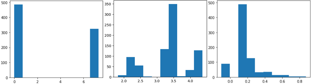
Figure 2: Diagonal costs learned for pairs of cells on the same row, column or sub-square, using the regular NPLL (left), the E-NPLL with $k=10$ (middle), and the Hinge loss (right). A positive cost shows a constraint has been learned. The NPLL shows many missed constraints. The E-NPLL learns all $810$ constraints, the Hinge loss omits some redundant ones (preserving $100\%$ test accuracy).

Multiple-solution grids.

Published Sudoku grids have only one solution. We now consider a Sudoku benchmark used in Nandwani et al. (2021), where each grid has more than one solution. For each grid, the set of solutions is only partially accessible during training: at most $5$ of them are present in the training set. The aim is to be able to predict any solution. We use $1,000$, $64$ and $256$ grids of the data set from Nandwani et al. (2021) respectively for training, validating, and testing. All hyper-parameters are set as previously, the validation set is only used to stop training. The testing criteria is to be able to retrieve one of the feasible solutions (all of them are known for testing).

Since the E-NPLL never compares a solver-produced solution to the provided solution $\mathbf{y}$, it is not sensitive to the existence of many solutions. With the same training procedure as previously, selecting one of the $5$ provided solutions randomly at each epoch, training takes $723.4\pm 64.9$ seconds ($21.4\pm 1.9$ epochs) on average, leading to one of the expected solutions for 100% of the test grids. In fact, since the correct rules are identified, we could verify that thresholding the learned costs into Boolean enables a complete enumeration of all feasible solutions for all instances in the test set.

5.2 Visual Sudoku

Our previous examples show the benefits of exploiting inputs $\omega$. To explore this capacity more deeply, we tackle the visual Sudoku problem in which hints are MNIST images. The goal is to simultaneously learn how to recognize digits and how to play Sudoku. We add a LeNet network Lecun et al. (1998) to our previous architecture. The GM $N(\omega$) produced is composed of the pairwise cost functions produced by the same Residual MLP with the addition of the negated logit output of LeNet as an elementary cost function on each variable $Y_{i}$ with a hint. This GM is fed to our regularized E-NPLL loss for back-propagating solutions. No new tuning is necessary (same learning rate for both networks).

Our data set is obtained from the symbolic Sudoku data set by replacing hints with corresponding MNIST images, as in Brouard et al. (2020). We use the same $1,000$ grids for training, the validation set contains $64$ grids (only used to stop training). To check for sensitivity to initialization (an 80% training failure rate was observed for SATNet in Chang et al. (2020)), $10$ runs with different seeds were performed.

After training, we extract the LeNet network alone: it reaches a $97.6$% accuracy on MNIST, being indirectly supervised by the provided hints, through the E-NPLL (directly in SATNet Chang et al. (2020)). We test again on $1,000$ hard grids (see Table 3). When all the hints are correctly predicted, grids are correctly filled, as proper rules have been learned. Moreover, in $8.7$% of cases, the solver is able to correct LeNet’s errors, leading to an overall accuracy of $76$% on hard grids. Training takes an average time of $1150\pm 13s$.

MNIST accuracy	Correct grids	Of which corrected
$97.6\pm 0.9$%	$760\pm 9$	$87\pm 3$

Table 3: Visual Sudoku performance ($1,000$ hard 17-hints test grids)

We also compare our architecture with SATNet, using their data set of 9K training and 1K easy test grids (average of $36.2$ hints Wang et al. (2019)). We use the exact same parameters as in the previous experiment and reuse SATNet’s ConvNet to process MNIST digits. We train for at most $20$ epochs ($100$ for SATNet) using $64$ of the training grids for validation (to decide when to stop training). On this data set, SATNet’s accuracy is $63.2$%. SATNet’s authors compared this to a theoretical maximum accuracy of $74.7\%$, using a $99.2\%$ accuracy MNIST classifier and a perfect Sudoku solver. Integrating LeNet’s uncertainty on classification as negated logits in the GM pushes accuracy well beyond this theoretical limit (see Table 4). Since the ConvNet is trained through the E-NPLL loss, its weights are automatically adjusted to optimize the joint Pseudo-Loglikelihood that includes also the Sudoku rules being learned. This automatically calibrates its output for the task (similarly to what is done, a posteriori and with known hard Sudoku rules, in Mulamba et al. (2020)).

SATNet	Theoretical	Ours
$63.2$ %	$74.2$%	$\mathbf{94.1}\pm 0.8$%

Table 4: Fraction of solved grids using SATNet data set for training and testing (averaged over 3 different initializations).

5.3 Learning To Design Proteins

The problem of designing proteins has similarities with solving Sudoku Strokach et al. (2020). Proteins are linear macro-molecules defined by a sequence of natural amino acids. Proteins usually fold into a specific 3D structure which enables specific biological or biochemical functions. Designed proteins have applications in health and green chemistry, among others Kuhlman and Bradley (2019). To design new proteins, with new functions or enhanced properties, one usually starts from an input backbone structure, matching the target functions, and predicts a sequence of amino acids that will fold onto the target structure.

Considering an input protein structure as a Sudoku grid, each amino acid corresponds to a cell and must be chosen among the $20$ natural amino acids instead of $9$ digits. The structure is predominantly determined by inter-atomic forces, which drive folding into a minimum energy geometry: the most usual approach of the protein design problem is as an NP-hard unconstrained energy minimization problem Pierce and Winfree (2002); Allouche et al. (2014). Inter-atomic forces are influenced by relative distances and atomic natures which implies that the final interactions inside a protein depend on the geometry of the input structure: we will therefore use this geometry in the natural inputs $\omega$, as we did with the (fixed) Sudoku grid geometry. Compared to Sudoku, protein design instances have variable geometry, they may contain several hundreds of amino acids or more and they are subjected to many-bodies interactions that cannot be directly represented in a pairwise GM.

When designing proteins, the Hamming distance between the predicted and observed (native) sequences, called the Native Sequence Recovery rate (NSR), is often used for evaluation. Protein design is a multiple-solution problem: above 30% of similarity, two protein sequences are considered as having the same fold (geometry). So, one given structure can adopt many sequences and a 100% NSR cannot be reached.

For training, we use the data set of Ingraham et al. (2019), already split into train/validation/test sets of respectively $17,000$, $600$ and $1,200$ proteins, in such a way that proteins with similar structures or sequences are in the same set. Similarly to Sudoku, a protein is described by features $\omega$ computed on each pair of positions $i,j$ in the protein. They include inter-atomic distance features encoded with Gaussian radial basis function Dauparas et al. (2022), and a positional encoding of the sequence distance ($|i-j|$) Vaswani et al. (2017). Each backbone geometry $\omega$ is associated with $\mathbf{y}$, the sequence of the corresponding known protein. All pair features in $\omega$ are processed by a neural network composed of a gated MLP Liu et al. (2021) that learns an environment embedding from a central amino acid and its neighbors within $10$Å, fed to a ResMLP (as for Sudoku) that takes pairs of features and environment embeddings to predict $20\times 20$ cost matrices. Training and architecture details are in annex C.

We train the same model with the same initialization using either the NPLL or the E-NPLL loss. To adapt to variable protein sizes, the E-NPLL eliminates $k$% of incoming neighbor messages. With up to $500$ amino acids, the optimization task is challenging at inference and we used a recent GM convex solver Durante et al. (2022). As shown in Table 5, we observe that the E-NPLL not only preserves the good properties of the NPLL but actually improves the NSR. While protein design is often stated as an unconstrained optimization problem, we hypothesize that this improvement results from the existence of infeasibilities: when local environments are very tight, they absolutely forbid large amino acids. Such infeasibilities could not be properly estimated by the NPLL alone.

k	0	10	40
NSR	40.6%	41.4%	42.9%

Table 5: Comparing the E-NPLL and the regular NPLL on the test proteins. Median NSR over the full test set are given. The case $k=0$ corresponds to the regular NPLL.

Our architecture provides a decomposable scoring function, such as those used for protein design in Rosetta Park et al. (2016). Table 6 compares both approaches on the data set of Park et al. (2016). We see that the E-NPLL learned decomposable scoring function outperforms Rosetta’s energy function. This is all the more satisfying as Rosetta’s full-atom function considers all atoms of the protein while we just use the backbone geometry and amino acids identities (as in coarse-grained scoring functions Kmiecik et al. (2016)).

	Rosetta	E-NPLL
NSR	17.9%	27.8%

Table 6: Comparison with the energy-based design method Rosetta on small single-chain proteins.

6 Conclusion

In this paper, we introduce a hybrid neural+graphical model architecture and a dedicated loss function for learning how to solve discrete reasoning problems. It is differentiable and as such, allows natural inputs to participate in the definition of discrete reasoning/optimization problems, providing the ability to inject suitable inductive biases that can also enhance data efficiency, as shown in the case of Sudoku. While most discrete/relaxed optimization layers Pogančić et al. (2020); Sahoo et al. (2023); Wang et al. (2019) can be inserted in an arbitrary position in a neural net, our final GM layer with the E-NPLL loss offers scalable training, avoiding calls to exact solvers that quickly struggle with the noisy instances that are predicted in early training epochs. It is able to benefit from exact or relaxed solvers during inference. Thanks to the E-NPLL, it can simultaneously identify a criterion to optimize as well as constraints. Finally, its output can be scrutinized to check properties and can be a posteriori completed with side constraints or additional criteria, in order to inject further instance-dependent information, that may have been learned, be available as knowledge or as user requirements.

On various NP-hard Sudoku benchmarks, it is able to produce correct solutions from natural input (including images), while being data-efficient and capable of generalization in incomplete multiple-solution settings. The use of an exact prover during inference results in robust prediction, allowing for the correction of otherwise noisy neural predictions. On the real-world protein design problem, our approach is also quickly able to learn a geometry-dependent pairwise decomposed function that outperforms the most recent full-atom pairwise decomposable energy functions for predicting the sequence of natural proteins.

Much remains to be done around this architecture. As for SATNet Lim et al. (2022), the ultimate $N(\omega)$ GM layer of our architecture could be analyzed during training to identify emerging hypothetical global properties such as symmetries or global decomposable constraints, allowing for more efficient learning and improved human understanding. For memory and computational efficiency, we limited ourselves to pairwise models but the use of other languages (e.g. weighted clauses) in replacement of, or addition to, pairwise functions would enhance the capacity of the architecture to capture many-bodies interactions. Another possibility is the use of latent/hidden variables Stergiou and Walsh (1999).

Appendix A On the Hinge loss

Property 3.

The Hinge loss for the Hamming loss with a $0$-margin is equivalent to the loss of Sahoo et al. (2023) with no projection.

When using the Hinge loss, the solver is embedded as a neural layer. For each sample $(\omega,\mathbf{y})$, the solver computes the optimal solution $\mathbf{y}^{*}$ of the predicted GM $N(\omega)$: $\mathbf{y}^{*}=\operatorname*{\arg\!\min}_{\mathbf{t}\in D^{\mathbf{Y}}}N(\omega)(\mathbf{t})$.

The observed $\mathbf{y}$ and the predicted solution $\mathbf{y}^{*}$ are compared using the Hamming loss.

$$\textit{Hamming}(\mathbf{y},\mathbf{y}^{*})=\sum_{i=1}^{n}\mathbb{1}[{y_{i}\neq y^{*}_{i}}]$$

This loss is discrete, therefore its gradient are uninformative (either $0$ or non-existent). To obtain meaningful gradients to back-propagate, the Hinge loss Tsochantaridis et al. (2005) provides an upper bound on the loss that is specifically easy to express for pairwise-decomposable losses $L$, such as the Hamming loss above.

$$\textit{Hinge}(\omega,\mathbf{y}) =\max_{\mathbf{t}\in D^{\mathbf{Y}}}\left[L(\mathbf{y},\mathbf{t})+(N(\omega)(\mathbf{y})-N(\omega)(\mathbf{t}))\right]$$

$$=N(\omega)(\mathbf{y})-\underbrace{\min_{\mathbf{t}\in D^{\mathbf{Y}}}\left[N(\omega)(\mathbf{t})-L(\mathbf{y},\mathbf{t})\right]}_{\operatorname*{\arg\!\min}=\mathbf{y}^{m}}$$

The Hamming loss can be simply computed as the cost of a CFN over $\mathbf{Y}$ with one cost function $F_{i}$ per variable $Y_{i}$ with $F_{i}(t_{i})=\mathbb{1}[t_{i}\neq y_{i}]$. The right minimization problem above can be therefore solved by calling the GM solver on the original problem $N(\omega)$ to which functions $-F_{i}$ scaled by factor $\alpha\geq 0$ (called the margin) have been added. If we denote by $\mathbf{y}^{m}$ the solution of this problem, for sample $(\omega,\mathbf{y})$, the Hinge loss will contain costs N$(\omega)[i,j](v_{i},v_{j})$ with a positive sign iff $v_{i}=y_{i}$ and $v_{j}=y_{j}$ (in $N(\omega)(\mathbf{y})$) and also with a negative sign iff $v_{i}=y^{m}_{i}$ and $v_{j}=y^{m}_{j}$ ($-N(\omega)(\mathbf{y}^{m})$). The only possibly non-zero gradient terms will be therefore $+1$ for $N(\omega)[i,j](y_{i},y_{j})$ and $-1$ for $N(\omega)[i,j](y^{m}_{i},y^{m}_{j})$ which will cancel iff $y_{i}=y^{m}_{i}$ and $y_{j}=y^{m}_{j}$. When looking at equation (2) from Sahoo et al. (2023), we obtain exactly the same gradients using $\alpha=0$. Therefore, the $0$-margin Hinge loss (also called the contrastive Viterbi loss or the perceptron loss LeCun et al. (2006)) is equivalent to the loss of  Sahoo et al. (2023) with no projection.

Appendix B Gradient of the NPLL

We have a data set $S$ composed of $m$ pairs $(\omega^{l},\mathbf{y}^{l}),1\leq l\leq m$. The Negative Pseudologlikelihood of $S$ is the sum of the negative log-probability of each $(\omega^{l},\mathbf{y}^{l})$:

$$NPLL(S) =\sum_{l=1}^{m}NPLL(\omega^{l},\mathbf{y}^{l})$$

$$=-\sum_{l=1}^{m}\left[\sum_{Y_{i}\in\mathbf{Y}}\log P^{N(\omega)}(y_{i}^{l}|\mathbf{y}^{l}_{-i})\right]$$

where

$$P^{N(\omega)}(y_{i}^{l}|\mathbf{y}^{l}_{-i})=\frac{\exp(-\sum_{j\neq i}N(\omega)[i,j](y^{l}_{i},y^{l}_{j}))}{\sum_{v_{i}\in D^{i}}\exp(-\sum_{j\neq i}N(\omega)[i,j](v_{i},y^{l}_{j}))}$$

The conditional probability above is obtained using the normalizing constant $Z^{N(\omega)}(\mathbf{y}^{l}_{-i})$ in the denominator:

$$Z^{N(\omega)}(\mathbf{y}^{l}_{-i})=\sum_{v_{i}\in D^{i}}\exp(-\sum_{j\neq i}N(\omega)[i,j](v_{i},y^{l}_{j}))$$

computed over all possible values $v_{i}$ of $Y_{i}$. This corresponds to the application of a softmax on the logits $-\sum_{j\neq i}N(\omega)[i,j](v_{i},y^{l}_{j})$.

Minimizing the NPLL means maximizing the probability above, therefore making $-N(\omega)[i,j](\cdot,y^{l}_{j})$ higher on the observed value $y^{l}_{i}$ (used in the numerator) than on the other values $v_{i}\neq y^{l}_{i}$ or equivalently, the cost $N(\omega)[i,j](\cdot,y^{l}_{j})$ lower on $y^{l}_{i}$ than on other values: the NPLL is a contrastive loss that seeks to create a margin between the values that are observed in the sample $S$ and the other values of the variable, for every variable and every sample.

Focusing on one pair $(\omega,\mathbf{y})\in S$ , we expand and get:

$$NPLL(\omega,\mathbf{y})=\\ -\sum_{Y_{i}\in\mathbf{Y}}\left[\left(-\sum_{j\neq i}N(\omega)[i,j](y_{i},y_{j})\right)-\log Z^{N(\omega)}(\mathbf{y}_{-i})\right]$$ (1)

The NPLL is a sum over all variables $Y_{i}\in\mathbf{Y}$ and we consider the contribution of a given variable $Y_{i}$. To compute the gradients of the corresponding term of the NPLL, we first compute the partial derivative of the logarithm of the normalizing constant $Z^{N(\omega)}(\mathbf{y}_{-i})$ ($i$ fixed) w.r.t. $N(\omega)[i,j](v_{i},y_{j})$ (for arbitrary $j\neq i$ and $v_{i}\in D^{i}$, other costs do not appear in $Z^{N(\omega)}(\mathbf{y}_{-i})$ and the corresponding partial derivative is $0$).

$$\frac{\partial\log Z^{N(\omega)}(\mathbf{y}_{-i})}{\partial N(\omega)[i,j](v_{i},y_{j})} =\frac{-\exp(-\sum_{k\neq i}N(\omega)[i,k](v_{i},y_{k}))}{Z^{N(\omega)}(\mathbf{y}_{-i})}$$

$$=-P^{N(\omega)}(v_{i}|\mathbf{y}_{-i})$$

For any $Y_{i}$, the partial derivative of the first term in equation 1 w.r.t. $N(\omega)[i,j](v_{i},v_{j})$ is $-\mathbb{1}(v_{i}=y_{i},v_{j}=y_{j})$.

Overall, given that $N(\omega)[i,j](v_{i},v_{j})$ and $N(\omega)[j,i](v_{j},v_{i})$ are the same, the contribution of sample $(\omega,\mathbf{y})$ to $\frac{\partial NPLL}{\partial N(\omega)[i,j](v_{i},v_{j})}$ will reduce to the non-zero contributions of variables $Y_{i}$ and $Y_{j}$:

$$\frac{\partial NPLL}{\partial N(\omega)[i,j](v_{i},v_{j})}=\\ [\mathbb{1}(y_{i}=v_{i},y_{j}=v_{j})-P^{N(\omega)}(v_{i}|\mathbf{y}_{-i})\mathbb{1}(y_{j}=v_{j})]\\ +[\mathbb{1}(y_{i}=v_{i},y_{j}=v_{j})-P^{N(\omega)}(v_{j}|\mathbf{y}_{-j})\mathbb{1}(y_{i}=v_{i})]$$

Appendix C Architecture and training details

For the protein design task, the neural network is composed of an input linear layer of size $128$, a gatedMLP with 15 layers, a width of $128*6=768$ and an output dimension of $64$, and a ResMLP with $20$ layers of $256$ neurons, with residual connections every $2$ layers. The gatedMLP consider the $45$ nearest neighbours of each residues. As in most protein energy functions Alford et al. (2017), amino acid pairs separated by a large distance are ignored. We use a $15$Å threshold.

The neural network is trained using the Adam optimizer, with a weight decay of $10^{-3}$ and an initial learning rate of $5.10^{-4}$, divided by $10$ when the validation loss decreases (with patience $0$) until it reaches $10^{-8}$. A L1 regularization of $10^{-4}$ is applied to costs.

To compare between the NPLL loss and the E-NPLL loss, we trained the same model with the same hyperparameters and starting from the same weight initialization with each of the loss. Both models run as long as the minimum LR is not reached, and therefore not necessarily for the same number of epochs.

References

- Alford et al. (2017) Rebecca F Alford, Andrew Leaver-Fay, Jeliazko R Jeliazkov, Matthew J O’Meara, Frank P DiMaio, Hahnbeom Park, Maxim V Shapovalov, P Douglas Renfrew, Vikram K Mulligan, Kalli Kappel, et al. The rosetta all-atom energy function for macromolecular modeling and design. Journal of chemical theory and computation, 13(6):3031–3048, 2017.
- Allouche et al. (2014) David Allouche, Isabelle André, Sophie Barbe, Jessica Davies, Simon de Givry, George Katsirelos, Barry O’Sullivan, Steve Prestwich, Thomas Schiex, and Seydou Traoré. Computational protein design as an optimization problem. Artificial Intelligence, 212:59–79, 2014.
- Allouche et al. (2015) David Allouche, Simon de Givry, George Katsirelos, Thomas Schiex, and Matthias Zytnicki. Anytime hybrid best-first search with tree decomposition for weighted csp. In International Conference on Principles and Practice of Constraint Programming, pages 12–29. Springer, 2015.
- Amos and Kolter (2017) Brandon Amos and J. Zico Kolter. OptNet: Differentiable optimization as a layer in neural networks. In Doina Precup and Yee Whye Teh, editors, Proceedings of the 34th International Conference on Machine Learning, volume 70 of Proceedings of Machine Learning Research, pages 136–145. PMLR, 06–11 Aug 2017.
- Beldiceanu and Simonis (2016) Nicolas Beldiceanu and Helmut Simonis. Modelseeker: Extracting global constraint models from positive examples. In Data Mining and Constraint Programming, pages 77–95. Springer, 2016.
- Berthet et al. (2020) Quentin Berthet, Mathieu Blondel, Olivier Teboul, Marco Cuturi, Jean-Philippe Vert, and Francis Bach. Learning with differentiable pertubed optimizers. In H. Larochelle, M. Ranzato, R. Hadsell, M.F. Balcan, and H. Lin, editors, Advances in Neural Information Processing Systems, volume 33, pages 9508–9519. Curran Associates, Inc., 2020.
- Besag (1975) Julian Besag. Statistical analysis of non-lattice data. Journal of the Royal Statistical Society: Series D (The Statistician), 24(3):179–195, 1975.
- Bessiere et al. (2017) Christian Bessiere, Frédéric Koriche, Nadjib Lazaar, and Barry O’Sullivan. Constraint acquisition. Artificial Intelligence, 244:315–342, 2017.
- Brouard et al. (2020) Céline Brouard, Simon de Givry, and Thomas Schiex. Pushing data into CP models using graphical model learning and solving. In International Conference on Principles and Practice of Constraint Programming, pages 811–827. Springer, 2020.
- Chang et al. (2020) Oscar Chang, Lampros Flokas, Hod Lipson, and Michael Spranger. Assessing SATNet's ability to solve the symbol grounding problem. In H. Larochelle, M. Ranzato, R. Hadsell, M.F. Balcan, and H. Lin, editors, Advances in Neural Information Processing Systems, volume 33, pages 1428–1439. Curran Associates, Inc., 2020.
- Cooper et al. (2020) Martin Cooper, Simon de Givry, and Thomas Schiex. Graphical models: queries, complexity, algorithms. In Symposium on Theoretical Aspects of Computer Science, Leibniz International Proceedings in Informatics, volume 154, pages 4–1, 2020.
- Dauparas et al. (2022) J. Dauparas, I. Anishchenko, N. Bennett, H. Bai, R. J. Ragotte, L. F. Milles, B. I. M. Wicky, A. Courbet, R. J. de Haas, N. Bethel, P. J. Y. Leung, T. F. Huddy, S. Pellock, D. Tischer, F. Chan, B. Koepnick, H. Nguyen, A. Kang, B. Sankaran, A. K. Bera, N. P. King, and D. Baker. Robust deep learning-based protein sequence design using proteinMPNN. Science, 378(6615):49–56, 2022.
- Demoen and de la Banda (2014) Bart Demoen and Maria Garcia de la Banda. Redundant sudoku rules. Theory and Practice of Logic Programming, 14(3):363–377, 2014.
- Durante et al. (2022) Valentin Durante, George Katsirelos, and Thomas Schiex. Efficient low rank convex bounds for pairwise discrete Graphical Models. In Thirty-ninth International Conference on Machine Learning, Baltimore, United States, July 2022.
- Elmachtoub and Grigas (2022) Adam N. Elmachtoub and Paul Grigas. Smart “predict, then optimize”. Management Science, 68(1):9–26, 2022.
- Geman and Graffigne (1986) Stuart Geman and Christine Graffigne. Markov random field image models and their applications to computer vision. In Proceedings of the international congress of mathematicians, volume 1, page 2. Berkeley, CA, 1986.
- He et al. (2016) Kaiming He, Xiangyu Zhang, Shaoqing Ren, and Jian Sun. Deep residual learning for image recognition. In Proceedings of the IEEE Conference on Computer Vision and Pattern Recognition (CVPR), June 2016.
- Ingraham et al. (2019) J. Ingraham, V. K. Garg, R. Barzilay, and T. Jaakkola. Generative models for graph-based protein design. In 33rd Conference on Neural Information Processing Systems (NeurIPS 2019), 2019.
- Kmiecik et al. (2016) Sebastian Kmiecik, Dominik Gront, Michal Kolinski, Lukasz Wieteska, Aleksandra Elzbieta Dawid, and Andrzej Kolinski. Coarse-grained protein models and their applications. Chemical Reviews, 116(14):7898–7936, 2016. PMID: 27333362.
- Kotary et al. (2021) James Kotary, Ferdinando Fioretto, Pascal Van Hentenryck, and Bryan Wilder. End-to-end constrained optimization learning: A survey. In Proc. of the 30 International Joint Conference on Artificial Intelligence, IJCAI 2021, IJCAI International Joint Conference on Artificial Intelligence, pages 4475–4482, 2021.
- Kuhlman and Bradley (2019) Brian Kuhlman and Philip Bradley. Advances in protein structure prediction and design. Nature Reviews Molecular Cell Biology, 20(11):681–697, 2019.
- Lecun et al. (1998) Y. Lecun, L. Bottou, Y. Bengio, and P. Haffner. Gradient-based learning applied to document recognition. Proceedings of the IEEE, 86(11):2278–2324, 1998.
- LeCun et al. (2006) Yann LeCun, Sumit Chopra, Raia Hadsell, M Ranzato, and Fujie Huang. A tutorial on energy-based learning. Predicting structured data, 1(0), 2006.
- Lim et al. (2022) Sangho Lim, Eun-Gyeol Oh, and Hongseok Yang. Learning symmetric rules with SATNet. In Proc. of NeurIPS’2022, 2022.
- Liu et al. (2021) Hanxiao Liu, Zihang Dai, David So, and Quoc V Le. Pay attention to MLPs. In M. Ranzato, A. Beygelzimer, Y. Dauphin, P.S. Liang, and J. Wortman Vaughan, editors, Advances in Neural Information Processing Systems, volume 34, pages 9204–9215. Curran Associates, Inc., 2021.
- Mandi and Guns (2020) Jayanta Mandi and Tias Guns. Interior point solving for LP-based prediction+ optimisation. Advances in Neural Information Processing Systems, 33:7272–7282, 2020.
- Mandi et al. (2020) Jayanta Mandi, Emir Demirovic, Peter J. Stuckey, and Tias Guns. Smart predict-and-optimize for hard combinatorial optimization problems. In Proceedings of the AAAI Conference on Artificial Intelligence, volume 34, pages 1603–1610, Apr. 2020.
- Mandi et al. (2022) Jayanta Mandi, Víctor Bucarey, Maxime Mulamba Ke Tchomba, and Tias Guns. Decision-focused learning: Through the lens of learning to rank. In Kamalika Chaudhuri, Stefanie Jegelka, Le Song, Csaba Szepesvari, Gang Niu, and Sivan Sabato, editors, Proceedings of the 39th International Conference on Machine Learning, volume 162 of Proceedings of Machine Learning Research, pages 14935–14947. PMLR, 17–23 Jul 2022.
- Montanari and Pereira (2009) Andrea Montanari and Jose Pereira. Which graphical models are difficult to learn? In Y. Bengio, D. Schuurmans, J. Lafferty, C. Williams, and A. Culotta, editors, Advances in Neural Information Processing Systems, volume 22. Curran Associates, Inc., 2009.
- Mulamba et al. (2020) Maxime Mulamba, Jayanta Mandi, Rocsildes Canoy, and Tias Guns. Hybrid classification and reasoning for image-based constraint solving. In International Conference on Integration of Constraint Programming, Artificial Intelligence, and Operations Research, pages 364–380. Springer, 2020.
- Nandwani et al. (2021) Yatin Nandwani, Deepanshu Jindal, Mausam ., and Parag Singla. Neural learning of one-of-many solutions for combinatorial problems in structured output spaces. In International Conference on Learning Representations, ICLR’21, 2021.
- Niepert et al. (2021) Mathias Niepert, Pasquale Minervini, and Luca Franceschi. Implicit MLE: Backpropagating through discrete exponential family distributions. In M. Ranzato, A. Beygelzimer, Y. Dauphin, P.S. Liang, and J. Wortman Vaughan, editors, Advances in Neural Information Processing Systems, volume 34, pages 14567–14579. Curran Associates, Inc., 2021.
- Palm et al. (2018) Rasmus Palm, Ulrich Paquet, and Ole Winther. Recurrent relational networks. In S. Bengio, H. Wallach, H. Larochelle, K. Grauman, N. Cesa-Bianchi, and R. Garnett, editors, Advances in Neural Information Processing Systems, volume 31. Curran Associates, Inc., 2018.
- Park et al. (2016) Hahnbeom Park, Philip Bradley, Per Greisen, Yuan Liu, Vikram Khipple Mulligan, David E. Kim, David Baker, and Frank DiMaio. Simultaneous optimization of biomolecular energy functions on features from small molecules and macromolecules. Journal of Chemical Theory and Computation, 12(12):6201–6212, 2016.
- Pierce and Winfree (2002) Niles A Pierce and Erik Winfree. Protein design is NP-hard. Protein engineering, 15(10):779–782, 2002.
- Pogančić et al. (2020) Marin Vlastelica Pogančić, Anselm Paulus, Vit Musil, Georg Martius, and Michal Rolinek. Differentiation of blackbox combinatorial solvers. In International Conference on Learning Representations, 2020.
- Sahoo et al. (2023) Subham Sekhar Sahoo, Anselm Paulus, Marin Vlastelica, Vít Musil, Volodymyr Kuleshov, and Georg Martius. Backpropagation through combinatorial algorithms: Identity with projection works. In Proc. of ICLR’23, 2023.
- Srivastava et al. (2014) Nitish Srivastava, Geoffrey Hinton, Alex Krizhevsky, Ilya Sutskever, and Ruslan Salakhutdinov. Dropout: a simple way to prevent neural networks from overfitting. The journal of machine learning research, 15(1):1929–1958, 2014.
- Stergiou and Walsh (1999) Kostas Stergiou and Toby Walsh. Encodings of non-binary constraint satisfaction problems. In Proc. AAAI’99, pages 163–168, 1999.
- Strokach et al. (2020) Alexey Strokach, David Becerra, Carles Corbi-Verge, Albert Perez-Riba, and Philip M. Kim. Fast and flexible protein design using deep graph neural networks. Cell Systems, 11(4):402–411.e4, 2020.
- Tsochantaridis et al. (2005) Ioannis Tsochantaridis, Thorsten Joachims, Thomas Hofmann, Yasemin Altun, and Yoram Singer. Large margin methods for structured and interdependent output variables. Journal of machine learning research, 6(9), 2005.
- Vaswani et al. (2017) Ashish Vaswani, Noam Shazeer, Niki Parmar, Jakob Uszkoreit, Llion Jones, Aidan N. Gomez, Lukasz Kaiser, and Illia Polosukhin. Attention is all you need. In 1st Conference on Neural Information Processing Systems (NIPS 2017), 2017.
- Wang et al. (2019) Po-Wei Wang, Priya Donti, Bryan Wilder, and Zico Kolter. SATNet: Bridging deep learning and logical reasoning using a differentiable satisfiability solver. In Kamalika Chaudhuri and Ruslan Salakhutdinov, editors, Proceedings of the 36th International Conference on Machine Learning, volume 97 of Proceedings of Machine Learning Research, pages 6545–6554. PMLR, 09–15 Jun 2019.
- Wilder et al. (2019) Bryan Wilder, Bistra Dilkina, and Milind Tambe. Melding the data-decisions pipeline: Decision-focused learning for combinatorial optimization. In Proceedings of the AAAI Conference on Artificial Intelligence, volume 33, pages 1658–1665, Jul. 2019.
- Zhang (2001) Weixiong Zhang. Phase transitions and backbones of 3-sat and maximum 3-sat. In International Conference on Principles and Practice of Constraint Programming, pages 153–167. Springer, 2001.