MoMo: Momentum Models for Adaptive Learning Rates

Abstract

Training a modern machine learning architecture on a new task requires extensive learning-rate tuning, which comes at a high computational cost. Here we develop new adaptive learning rates that can be used with any momentum method, and require less tuning to perform well. We first develop MoMo, a Momentum Model based adaptive learning rate for SGD-M (Stochastic gradient descent with momentum). MoMo uses momentum estimates of the batch losses and gradients sampled at each iteration to build a model of the loss function. Our model also makes use of any known lower bound of the loss function by using truncation, e.g. most losses are lower-bounded by zero. We then approximately minimize this model at each iteration to compute the next step. We show how MoMo can be used in combination with any momentum-based method, and showcase this by developing MoMo-Adam - which is Adam with our new model-based adaptive learning rate. Additionally, for losses with unknown lower bounds, we develop on-the-fly estimates of a lower bound, that are incorporated in our model. Through extensive numerical experiments, we demonstrate that MoMo and MoMo-Adam improve over SGD-M and Adam in terms of accuracy and robustness to hyperparameter tuning for training image classifiers on MNIST, CIFAR10, CIFAR100, Imagenet, recommender systems on the Criteo dataset, and a transformer model on the translation task IWSLT14.

1 Introduction

Training of a modern production-grade large neural network can cost over $1$ million dollars in compute. For instance, the cost for the Text-to-Text Transfer Transformer T5-model (Raffel et al., 2020) is estimated to be more than $1.3$ million dollars for a single run (Sharir et al., 2020). What makes training models so expensive is that multiple runs are needed to tune the hyperparameters, with arguably the most important parameter being the learning rate. Indeed, finding a good learning-rate schedule plays a disproportionately large role in the resulting test error of the model, with one extensive study showing that it was at least as important as the choice of optimizer (Schmidt et al., 2021).

Here, we develop adaptive learning rates that can be used together with any momentum-based method. To showcase our method, we apply our learning rates to SGD-M (Stochastic Gradient Descent with momentum) and to Adam (Kingma and Ba, 2015), which gives the MoMo and MoMo-Adam method, respectively. We make use of model-based stochastic optimization (Asi and Duchi, 2019; Davis and Drusvyatskiy, 2019; Chadha et al., 2021), and leverage that loss functions are bounded below (typically by zero) to derive our new MoMo (Model-based Momentum) adaptive learning rate.

1.1 The Model-Based Approach

Consider the problem

$$\min_{x\in\mathbb{R}^{d}}\;f(x),\quad f(x):=\mathbb{E}_{s\sim{\cal D}}\left[f(x,s)\right],$$ (1)

where $f(x,s)$ is a loss function, $s$ is an input (mini-batch of data), and $x$ are the parameters of a model we are trying to fit to the data. We assume throughout that $f(x,s)\geq 0$, which is the case for most loss functions. We also assume that $f(\cdot,s)$ is continuously differentiable for all $s\in{\cal D}$, that there exists a solution $x^{*}$ to (1) and denote the optimal value by $f^{*}\coloneqq f(x^{*})\in\mathbb{R}$.

In our main algorithms MoMo and MoMo-Adam (Algorithms 1 and 2), we present adaptive learning rates for SGD-M and Adam, respectively. To derive MoMo and MoMo-Adam, we use the model-based viewpoint, which is often motivated by the Stochastic Proximal Point (SPP) (Asi and Duchi, 2019; Davis and Drusvyatskiy, 2019) method. At each iteration, SPP samples $s_{k}\sim{\cal D},$ then trades-off minimizing $f(x,s_{k})$ with not moving too far from the current iterate $x^{k}$. Given a learning rate $\alpha_{k}>0$, this can be written as

$$x^{k+1}=\underset{x\in\mathbb{R}^{d}}{\operatorname{argmin}}\;f(x,s_{k})+\frac{1}{2\alpha_{k}}\left\|x-x^{k}\right\|^{2}.$$ (2)

Since this problem needs to be solved at every iteration, it needs to be fast to compute. However, in general (2) is difficult to solve because $f(x,s_{k})$ can be a highly nonlinear function. Model-based methods replace $f(x,s_{k})$ by a simple model $m_{k}(x)$ of the function (Asi and Duchi, 2019; Davis and Drusvyatskiy, 2019), and update according to

$$x^{k+1}\;=\;\underset{x\in\mathbb{R}^{d}}{\operatorname{argmin}}\;m_{k}(x)+\frac{1}{2\alpha_{k}}\left\|x-x^{k}\right\|^{2}.$$ (3)

SGD can be formulated as a model-based method by choosing the model to be the linearization of $f(x,s_{k})$ around $x^{k},$ that is

$$m_{k}(x)\;=\;f(x^{k},s_{k})+\left<\nabla f(x^{k},s_{k}),x-x^{k}\right>.$$ (4)

Using the above $m_{k}(x)$ in (3) gives the SGD update $x^{k+1}=x^{k}-\alpha_{k}\nabla f(x^{k},s_{k})$, see (Robbins and Monro, 1951; Asi and Duchi, 2019).

Our main insight for developing the MoMo methods is that we should build a model directly for $f(x)$, and not $f(x,s_{k})$, since our objective is to minimize $f(x)$. To this end, we develop a model $m_{k}(x)$ that is a good approximation of $f(x)$ when $x$ is close to $x^{k}$, and such that (3) has a simple closed form solution. Our model uses momentum estimates of past gradients and loss values to build a model $f(x)$. Finally, since the loss function is positive, we also impose that our model be positive.

1.2 Background and Contributions

Momentum and model-based methods.

The update formula of many stochastic methods such as SGD can be interpreted by taking a proximal step with respect to a model of the objective function (Asi and Duchi, 2019; Davis and Drusvyatskiy, 2019). Independently of this, (heavy-ball) momentum (Polyak, 1964; Sebbouh et al., 2021) is incorporated into many methods in order to boost performance.

Contributions. Here we give a new model-based interpretation of momentum, namely that it can be motivated as a model of the objective function $f(x)$ by averaging sampled loss functions. This allows us to naturally combine momentum with other model-based techniques.

Lower bounds and truncated models.

One of the main advantages of the model-based viewpoint (Asi and Duchi, 2019; Davis and Drusvyatskiy, 2019) is that it illustrates how to use knowledge of a lower bound of the function via truncation. Methods using this truncated model are often easier to tune (Meng and Gower, 2023; Schaipp et al., 2023).

Contributions. By combining the model-based viewpoint of momentum with a truncated model we arrive at our new MoMo method. Since we are interested in loss functions, we can use zero as a lower bound estimate in many learning tasks. However, for some tasks such as training transformers, the minimal loss is often non-zero. If the non-zero lower bound is known, we can straightforwardly incorporate it into our model. For unknown lower bound values we also develop new online estimates of a lower bound in Section 4. Our estimates can be applied to any stochastic momentum-based method, and thus may be of independent interest. Our main influence for this development was D-adaptation (Defazio and Mishchenko, 2023) which develops an online estimate of the distance to the solution.

Adaptive methods.

In practice, tuning learning-rate schedules is intricate and computationally expensive. Adam  (Kingma and Ba, 2015) and variants such as AdamW (Loshchilov and Hutter, 2019), are often easier to tune and are now being used routinely to train DNNs across a variety of tasks. This and the success of Adam have incentivised the development of many new adaptive learning rates, including approaches based on coin-betting  (Orabona and Tommasi, 2017), variants of AdaGrad (Duchi et al., 2011; Defazio and Mishchenko, 2023), and stochastic line search (Vaswani et al., 2019). Recent work also combines parameter-free coin betting methods with truncated models (Chen et al., 2022).

Contributions. Our new adaptive learning rate can be combined with any momentum based method, and even allows for a preconditioner to be used. For example, Adam is a momentum method that makes use of a preconditioner. By using this viewpoint, together with a lower bound, we derive MoMo-Adam, a variant of Adam that uses our adaptive learning rates.

Adaptive Polyak step sizes.

For convex, non-smooth optimization, Polyak proposed an adaptive step size using the current objective function value $f(x^{k})$ and the optimal value $f^{*}$ (Polyak, 1987). Recently, the Polyak step size has been adapted to the stochastic setting (Berrada et al., 2020; Gower et al., 2021; Loizou et al., 2021; Orvieto et al., 2022). For example, (Loizou et al., 2021) proposed

$$x^{k+1}=x^{k}-\min\Big{\{}\gamma_{b},\tfrac{f(x^{k},s_{k})-\inf_{z}f(z,s_{k})}{c\|\nabla f(x^{k},s_{k})\|^{2}}\Big{\}}\nabla f(x^{k},s_{k}),$$ (SPS_max)

called the SPS_max method, where $c,\gamma_{b}>0$. The stochastic Polyak step size is closely related to stochastic model-based proximal point methods as well as stochastic bundle methods (Asi and Duchi, 2019; Paren et al., 2022; Schaipp et al., 2023).

Contributions. Our proposed method MoMo can be seen as an extension of the Polyak step size that also incorporates momentum. This follows from the viewpoint of the Polyak step size (Berrada et al., 2020; Paren et al., 2022; Schaipp et al., 2023) as a truncated model-based method. In particular MoMo with no momentum is equal to SPS_max.

Numerical findings.

We find that MoMo consistently improves the sensitivity with respect to hyperparameter choice as compared to SGD-M for standard image classification tasks including MNIST, CIFAR10, CIFAR100 and Imagenet. The same is true for MoMo-Adam compared to Adam on encoder-decoder transformers on the translation task IWSLT14.

Furthermore, we observe that the adaptive learning rate of MoMo(-Adam) for some tasks automatically performs a warm-up at the beginning of training and a decay in later iterations, two techniques often used in order to improve training (Sun, 2020).

2 Model-Based Momentum Methods

Let us recall the SGD model in (4) which has two issues: First, it approximates a single stochastic function $f(x,s_{k})$, as opposed to the full loss $f(x)$. Second, this model can be negative even though our loss function is always positive. Here, we develop a model directly for $f(x)$, and not $f(x,s_{k}),$ which also takes into account lower bounds on the function value.

2.1 Model-Based Viewpoint of Momentum

Suppose we have sampled inputs $s_{1},\ldots,s_{k}$ and past iterates $x^{1},\ldots,x^{k}$. We can use these samples to build a better model of $f(x)$ by averaging past function evaluations as follows

$$f(x)=\mathbb{E}_{s\sim{\cal D}}\left[f(x,s)\right]\;\approx\;\tfrac{1}{\rho_{k}}\sum_{j=1}^{k}\rho_{j,k}f(x,s_{j}),$$ (5)

where $\rho_{j,k}\geq 0$ and $\rho_{k}:=\sum_{j=1}^{k}\rho_{j,k}$. Thus, the $\rho_{k}^{-1}\rho_{j,k}$ are a discrete probability mass function over the previous samples. The issue with (5) is that it is expensive to evaluate $f(x,s_{j})$ for $j=1,\ldots,k$, which we would need to do at every iteration. Instead, we approximate each $f(x,s_{j})$ by linearizing $f(x,s_{j})$ around $x^{j}$, the point it was last evaluated

$$f(x,s_{j})\approx f(x^{j},s_{j})+\left<\nabla f(x^{j},s_{j}),x-x^{j}\right>,\quad\mbox{for }j=1,\ldots,k.$$ (6)

Using (5) and the linear approximations in (6) we can approximate $f(x)$ as follows

$$f(x)\approx\tfrac{1}{\rho_{k}}\sum_{j=1}^{k}\rho_{j,k}\big{(}f(x^{j},s_{j})+\left<\nabla f(x^{j},s_{j}),x-x^{j}\right>\big{)}=m_{k}(x).$$ (7)

If we use the above model $m_{k}(x)$ in (3), then the resulting update is SGD-M

$$x^{k+1}\;=x^{k}-\frac{\alpha_{k}}{\rho_{k}}d_{k},\quad\mbox{where }\;\textstyle d_{k}\coloneqq\sum_{j=1}^{k}\rho_{j,k}\nabla f(x^{j},s_{j}).$$ (8)

This gives a new viewpoint of momentum. Next we incorporate a lower bound into this model so that, much like the loss function, it cannot become negative.

2.2 Deriving MoMo

Since we know the loss is lower-bounded by zero, we will also impose a lower bound on the model (7). Though we could use zero, we will use an estimate $f_{*}^{k}\geq 0$ of the lower bound to allow for cases where $f(x^{*})$ may be far from zero. Imposing a lower bound of $f_{*}^{k}$ gives the following model

$$\textstyle f(x)\approx\max\Big{\{}\tfrac{1}{\rho_{k}}\sum_{j=1}^{k}\rho_{j,k}\big{(}f(x^{j},s_{j})+\left<\nabla f(x^{j},s_{j}),x-x^{j}\right>\big{)},f_{*}^{k}\Big{\}}=:m_{k}(x).$$ (9)

For overparametrized machine-learning models the minimum value $f(x^{*})$ is often close to zero (Ma et al., 2018; Gower et al., 2021). Thus, choosing $f_{*}^{k}=0$ in every iteration will work well (as we verify later in our experiments). For tasks where $f_{*}^{k}=0$ is too loose of a bound, in Section 4 we develop an online estimate for $f_{*}^{k}$ based on available information. Using the model (9), we can now define the proximal update

$$x^{k+1}=\underset{y\in\mathbb{R}^{d}}{\operatorname{argmin}}\;m_{k}(y)+\frac{1}{2\alpha_{k}}\|y-x^{k}\|^{2}.$$ (10)

Because $m_{k}(y)$ is a simple piece-wise linear function, the update (10) has a closed form solution, as we show in the following lemma (proof in Section C.1).

Lemma 2.1.

[MoMo update] Let

$$d_{k}\coloneqq\sum_{j=1}^{k}\rho_{j,k}\nabla f(x^{j},s_{j}),\quad\bar{f}_{k}:=\sum_{j=1}^{k}\rho_{j,k}f(x^{j},s_{j}),\quad\gamma_{k}:=\sum_{j=1}^{k}\rho_{j,k}\langle\nabla f(x^{j},s_{j}),x^{j}\rangle.$$ (11)

Using model (9), the closed form solution to (10) is

$$x^{k+1}=x^{k}-\tau_{k}d_{k},\quad\tau_{k}:=\min\Big{\{}\tfrac{\alpha_{k}}{\rho_{k}},\tfrac{\big{(}\bar{f}_{k}+\left<d_{k},x^{k}\right>-\gamma_{k}-\rho_{k}f_{*}^{k}\big{)}_{+}}{\|d_{k}\|^{2}}\Big{\}}.$$ (12)

Finally, it remains to select the averaging coefficients $\rho_{j,k}$. Here we will use an exponentially weighted average that places more weight on recent samples. Aside from working well in practice on countless real-world examples, exponential averaging can be motivated through the model-based interpretation. Recent iterates will most likely have gradients, and loss values, that are closer to our current iterate $x^{k}$. Thus we place more weight on recent iterates i.e. $\rho_{j,k}$ big for $j$ close to $k$. We give two options for exponentially weighted averaging next.

2.3 The Coefficients $\rho_{j,k}$: To bias or not to bias

We now choose $\rho_{j,k}\geq 0$ such that we can update $\bar{f}_{k}$, $d_{k}$ and $\gamma_{k}$ in (11) on the fly, storing only two scalars and one vector, and with the same resulting iteration complexity as SGD-M.

Exponentially Weighted Average. Let $\beta\in[0,1)$. Starting with $\rho_{1,1}=1$, and for $k\geq 2$ define $\rho_{j,k}=\beta\rho_{j,k-1}$ for $j\leq k-1$ and $\rho_{j,k}=1-\beta$ for $j=k$. Then, $\rho_{k}=\sum_{j=1}^{k}\rho_{j,k}=1$ for all $k\in\mathbb{N}$ and the quantities in (11) are exponentially weighted averages, see Lemma A.1. As a consequence, we can update $\bar{f}_{k}$, $d_{k}$ and $\gamma_{k}$ on the fly as given in lines 1–1 in Algorithm 1. Combining update (12) and the fact that $\rho_{k}=1$, we obtain Algorithm 1, which we call MoMo.

1 Default settings: $\alpha_{k}=1$, $\beta=0.9$, $(f_{*}^{k})_{k\in\mathbb{N}}=0.$

Input: $x^{1}\in\mathbb{R}^{d}$, $\beta\in[0,\;1)$, $\alpha_{k}>0,(f_{*}^{k})_{k\in\mathbb{N}}\subset\mathbb{R}$

2 Init:$\bar{f}_{0}=f(x^{1},s_{1}),d_{0}=\nabla f(x^{1},s_{1})$,$\gamma_{0}=\left<d_{0},x^{1}\right>$

3for $k=1$ to $K-1$ do

4       $\displaystyle\bar{f}_{k}\;=(1-\beta)f(x^{k},s_{k})+\beta\bar{f}_{k-1}$

5      $\displaystyle\gamma_{k}=(1-\beta)\left<\nabla f(x^{k},s_{k}),x^{k}\right>+\beta\gamma_{k-1}$

6      $\displaystyle d_{k}\;=(1-\beta)\nabla f(x^{k},s_{k})+\beta d_{k-1}$

7      $\displaystyle h_{k}\;=\bar{f}_{k}+\left<d_{k},x^{k}\right>-\gamma_{k}$

8      $\displaystyle x^{k+1}=x^{k}-\min\Big{\{}\alpha_{k},\tfrac{(h_{k}-f_{*}^{k})_{+}}{\|d_{k}\|^{2}}\Big{\}}d_{k}$

Output: $x^{K}$

Algorithm 1 MoMo: Model-based Momentum method.

Remark 2.2.

The adaptive learning rate $\tau_{k}$ in (12) determines the size of the step and can vary in each iteration even if $\alpha_{k}$ is constant. The (user-specified) learning rate $\alpha_{k}$ caps the adaptive learning rate.

Remark 2.3 (Complexity).

MoMo has the same order iteration complexity and memory footprint as SGD-M. MoMo stores two additional scalars $\gamma_{k}$ and $\bar{f}_{k}$, as compared to SGD-M, and has two additional ${\cal O}(d)$ inner products lines 5 and 7, and one ${\cal O}(d)$ vector norm on line 8.

For $\beta=0$ (no momentum), we have $\gamma_{k}=\langle\nabla f(x^{k},s_{k}),x^{k}\rangle=\langle d_{k},x^{k}\rangle$ and $\bar{f}_{k}=f(x^{k},s_{k}).$ Consequently $h_{k}=f(x^{k},s_{k})$, and in this special case, MoMo is equivalent to (SPS_max).

Fig. 1 shows how the MoMo model (10) approximates a convex function (left) and a non-convex function (right). The MoMo update $x_{{\texttt{MoMo}}{}}^{k+1}$ in Fig. 1 is closer to the minima (left) and sometimes much closer (right) on non-convex problems, as compared the SGD-M update.

Averaging with Bias Correction.

Alternatively, we can choose $\rho_{j,k}=(1-\beta)\beta^{k-j}$ for $j=1,\ldots,k$, as it is used in Adam (Kingma and Ba, 2015). This gives $\rho_{k}=1-\beta^{k}\neq 1$. We discuss this choice for MoMo in Section A.1 and will use it later for MoMo-Adam.

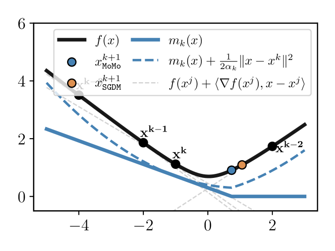
(a) Convex loss

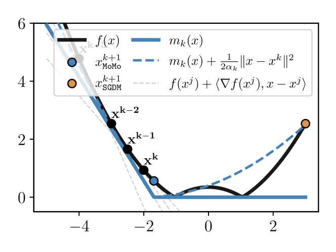
(b) Non-convex loss

Figure 1: Illustration of the MoMo model (blue curves) for two different loss functions with $\alpha_{k}=5$. Due to truncation, the new iterate of MoMo (blue point) is closer to the minimum than SGD-M (orange point). The right plot shows how MoMo takes a small step when gradients are steep, whereas SGD-M takes a large step and ends up far from the solution.

3 Weight Decay and Preconditioning

Often weight decay is used in order to improve generalization (Zhang et al., 2019). Weight decay is equivalent to adding a squared $\ell_{2}$-regularization to the objective function (Krogh and Hertz, 1991), in other words, instead of (1) we solve $\min_{x\in\mathbb{R}^{d}}f(x)+\tfrac{\color[rgb]{0,0,0}{\lambda}}{2}\left\|x\right\|^{2}$, where $f(x)$ is again the loss function. To include weight decay, we build a model $m_{k}$ for the loss $f$ and keep the $\ell_{2}$-regularization outside of the model. That is equation (10) is modified to

$$x^{k+1}=\underset{\scriptsize y\in\mathbb{R}^{d}}{\operatorname{argmin}}\;m_{k}(y)+\frac{\color[rgb]{0,0,0}{\lambda}}{2}\|y\|^{2}+\frac{1}{2\alpha_{k}}\|y-x^{k}\|^{2}.$$ (13)

Finally, the Euclidean norm may often not be best suited. Many popular methods such as AdaGrad or Adam are based on using a preconditioner for the proximal step. Hence, we allow for an arbitrary norm defined by a symmetric, positive definite matrix ${\color[rgb]{0,0,0}{\bf D}_{k}}\in\mathbb{R}^{d\times d}$, i.e. $\left\|x\right\|_{{\color[rgb]{0,0,0}{\bf D}_{k}}}^{2}:=\langle{\color[rgb]{0,0,0}{\bf D}_{k}}x,x\rangle.$ We can now use ${\color[rgb]{0,0,0}{\bf D}_{k}}$ to change the metric within our proximal method

$$x^{k+1}=\underset{y\in\mathbb{R}^{d}}{\operatorname{argmin}}\;m_{k}(y)+\frac{\color[rgb]{0,0,0}{\lambda}}{2}\|y\|_{{\color[rgb]{0,0,0}{\bf D}_{k}}}^{2}+\frac{1}{2\alpha_{k}}\|y-x^{k}\|_{{\color[rgb]{0,0,0}{\bf D}_{k}}}^{2}.$$ (14)

This update (14) enjoys the following closed form solution (proof in Section C.2).

Lemma 3.1.

Using model (9), the closed form solution to (14) is given by

$$\tau_{k} =\min\Big{\{}\frac{\alpha_{k}}{\rho_{k}},\frac{\big{(}(1+\alpha_{k}{\color[rgb]{0,0,0}{\lambda}})(\bar{f}_{k}-\rho_{k}f_{*}^{k}-\gamma_{k})+\langle d_{k},x^{k}\rangle\big{)}_{+}}{\|d_{k}\|_{{\color[rgb]{0,0,0}{\bf D}_{k}^{-1}}}^{2}}\Big{\}},$$ (15)

$$x^{k+1} =\tfrac{1}{1+\alpha_{k}\color[rgb]{0,0,0}{\lambda}}\Big{[}x^{k}-\tau_{k}{\color[rgb]{0,0,0}{\bf D}_{k}^{-1}}d_{k}\Big{]}.$$ (16)

Lemma 3.1 shows how to incorporate weight decay in MoMo: we replace Algorithm 1 in Algorithm 1 by (16) with ${\color[rgb]{0,0,0}{\bf D}_{k}}=\mathbf{Id}$ and $\rho_{k}=1$. If $\beta=0$ (no momentum) then MoMo with weight decay recovers ProxSPS, the proximal version of the stochastic Polyak step (Schaipp et al., 2023).

Deriving MoMo-Adam.

Using Lemma 3.1 we can obtain an Adam-version of MoMo by defining ${\color[rgb]{0,0,0}{\bf D}_{k}}$ as the diagonal preconditioner of Adam. Let $\mathbf{1}_{d}$ be the $d$-dimensional vector of ones, $\mathrm{Diag}(v)$ a diagonal matrix with diagonal entries $v\in\mathbb{R}^{d}$, and $\odot$ and $\sqrt{v}$ the elementwise multiplication and square-root operations. Denoting $g_{k}=\nabla f(x^{k},s_{k})$, we choose

$$v_{k}=(1-\beta_{2})v_{k-1}+\beta_{2}(g_{k}\odot g_{k}),\quad{\color[rgb]{0,0,0}{\bf D}_{k}}=\mathrm{Diag}(\epsilon\mathbf{1}_{d}+\sqrt{v_{k}/(1-\beta_{2})^{k}}),$$

where $\beta_{2}\in[0,1),~{}\epsilon>0$. Using this preconditioner with Lemma 3.1 gives Algorithm 2, called MoMo-Adam. Note that here we choose $\rho_{j,k}=(1-\beta)\beta^{k-j}$ (cf.  Section 2.3) which gives the standard averaging scheme of Adam. We focus on MoMo versions of SGD-M and Adam because these are the two most widely used methods. However, from Lemma 3.1 we could easily obtain a MoMo-version of different variations, such as Adabelief (Zhuang et al., 2020).

1 Default settings: $\alpha_{k}=10^{-2}$, $(\beta_{1},\beta_{2})=(0.9,0.999)$, $\epsilon=10^{-8}$

Input: $x^{1}\in\mathbb{R}^{d}$, $\beta_{1},\beta_{2}\in[0,\;1)$, $\epsilon>0$, $\alpha_{k}>0$, ${\color[rgb]{0,0,0}{\lambda}}\geq 0$, and $(f_{*}^{k})_{k\in\mathbb{N}}\subset\mathbb{R}$.

2 Initialize: $\bar{f}_{0}=0,d_{0}=0$, $\gamma_{0}=0$, and $v_{0}=0$.

3for $k=1$ to $K-1$ do

4      

5      $\displaystyle g_{k}\;=\nabla f(x^{k},s_{k});\quad d_{k}\;=(1-\beta_{1})g_{k}+\beta_{1}d_{k-1}$

6      $\displaystyle v_{k}\;=\beta_{2}v_{k-1}+(1-\beta_{2})(g_{k}\odot g_{k})$

7      ${\color[rgb]{0,0,0}{\bf D}_{k}}\;=\mathrm{Diag}\big{(}\epsilon\mathbf{1}_{d}+\sqrt{\left.v_{k}\right/(1-\beta_{2}^{k})}\big{)}$

8      $\displaystyle\bar{f}_{k}\;=(1-\beta_{1})f(x^{k},s_{k})+\beta_{1}\bar{f}_{k-1}$

9      $\displaystyle\gamma_{k}=(1-\beta_{1})\left<g_{k},x^{k}\right>+\beta_{1}\gamma_{k-1}$

10      $\tau_{k}\;=\min\Big{\{}\frac{\alpha_{k}}{1-\beta_{1}^{k}},\frac{\big{(}(1+{\color[rgb]{0,0,0}\lambda}\color[rgb]{0,0,0}\alpha_{k})(\bar{f}_{k}-\gamma_{k}-(1-\beta_{1}^{k})f_{*}^{k})+\left<d_{k},x^{k}\right>\big{)}_{+}}{\|d_{k}\|_{{\color[rgb]{0,0,0}{\bf D}_{k}^{-1}}}^{2}}\Big{\}}$

11      $x^{k+1}=\tfrac{1}{1+\alpha_{k}{\color[rgb]{0,0,0}{\lambda}}}\left[x^{k}-\tau_{k}{\color[rgb]{0,0,0}{\bf D}_{k}^{-1}}d_{k}\right]$

Output: $x^{K}$

Algorithm 2 MoMo-Adam: Adaptive learning rates for Adam

4 Estimating a Lower Bound

So far, we have assumed that lower-bound estimates $(f_{*}^{k})$ are given with $f_{*}^{k}=0$ being the default. However, this might not be a tight estimate of $f^{*}$ (e.g. when training transformers). In such situations, we derive an online estimate of the lower bound. In particular, for convex functions we will derive a lower bound for an unbiased estimate of $f(x^{*})$ given by

$$\bar{f}^{k}_{*}:= \tfrac{1}{\rho_{k}}\mbox{$\sum_{j=1}^{k}$}\rho_{j,k}f(x^{*},s_{j}),\quad\mbox{where}\quad\mathbb{E}\left[\bar{f}^{k}_{*}\right]=f(x^{*}).$$ (17)

Though $\bar{f}^{k}_{*}$ is not equal to $f(x^{*})$, it is an unbiased estimate since $\mathbb{E}\left[f(x^{*},s_{j})\right]=f(x^{*})$. It is also a reasonable choice since we motivated our method using the analogous approximation of $f(x)$ in (5). Furthermore, if $f_{*}^{k}=\bar{f}^{k}_{*}$ then for any preconditioner and convex losses, an iterate of MoMo can only decrease the distance to a given optimal point, as we show next.

Lemma 4.1.

Let $f(\cdot,s)$ be convex for every $s$ and let $x^{*}\in\arg\min_{x\in\mathbb{R}^{d}}f(x)$. For the iterates of the general MoMo update (cf. Lemma 3.1) with $\lambda=0$ and $f_{*}^{k}=\bar{f}^{k}_{*}$, it holds

$$\left\|x^{k+1}-x^{*}\right\|_{{\bf D}_{k}}^{2}\leq\left\|x^{k}-x^{*}\right\|_{{\bf D}_{k}}^{2}-\tau_{k}(h_{k}-\rho_{k}\bar{f}^{k}_{*})_{+}.$$ (18)

We use this monotonicity to derive a convergence theorem for MoMo in Theorem F.2. The following lemma derives an estimate $f_{*}^{k}\geq 0$ for $\bar{f}^{k}_{*}$ given in (17) by using readily available information for any momentum-based method, such as Algorithm 2.

Lemma 4.2.

Let $f(x,s)$ be convex in $x$ for all $s\in\cal D$. Let $x^{k}$ be given by (16) with $\lambda=0$. Let $\eta_{k}:=\prod_{j=2}^{k}\lambda_{\min}\big{(}{\bf D}_{j}^{-1}{\bf D}_{j-1}\big{)},$ and $h_{k}:=\bar{f}_{k}+\langle d_{k},x^{k}\rangle-\gamma_{k}$. We have $\bar{f}_{*}^{k}\geq f_{*}^{k+1}$ where

$$f_{*}^{k+1}\coloneqq\tfrac{1}{2\eta_{k}\tau_{k}\rho_{k}}\Big{(}\mbox{$\sum_{j=1}^{k}2\eta_{j}\tau_{j}\left(h_{j}-\tfrac{1}{2}\tau_{j}\left\|d_{j}\right\|_{{\bf D}_{j}^{-1}}^{2}\right)-D_{1}^{2}-2\sum_{j=1}^{k-1}\eta_{j}\tau_{j}\rho_{j}\bar{f}_{*}^{j}$}\Big{)}$$

where $D_{1}:=\left\|x^{1}-x^{*}\right\|_{{\bf D}_{1}}.$ Bootstrapping by using $f^{k}_{*}\approx\bar{f}_{*}^{k-1}$ we have for $k\geq 2$ that

$$f_{*}^{k+1} =\;\frac{1}{\rho_{k}}\left(h_{k}-\tfrac{1}{2}\tau_{k}\left\|d_{k}\right\|_{{\bf D}_{k}^{-1}}^{2}\right).$$ (19)

To simplify the discussion, consider the case without a preconditioner, i.e. ${\bf D}_{k}=\mathbf{Id}$, thus $\eta_{k}=1$. First, note that $f_{*}^{k+1}$ depends on the initial distance to the solution $D_{1}$, which we do not know. Fortunately, $D_{1}$ does not appear in the recursive update (19), because it only appears in $f^{1}_{*}.$ We can circumvent this initial dependency by simply setting $f^{1}_{*}=0.$

We need one more precautionary measure, because we cannot allow the step size $\tau_{k}$ in (15) to be zero. That is, by examining (15) we have to disallow that

$$(1+\alpha_{k}\lambda)\rho_{k}f_{*}^{k}\geq(1+\alpha_{k}\lambda)(\bar{f}_{k}-\gamma_{k})+\langle d_{k},x^{k}\rangle=:h_{k}^{\lambda}.$$ (20)

Hence, in each iteration of MoMo or MoMo-Adam, we call the ResetStar routine in Algorithm 3 before the update of $x^{k+1}$ that checks if this upper bound has been crossed, and if so, resets $f_{*}^{k}$ to be sufficiently small. After updating $x^{k+1}$, we update $f_{*}^{k+1}$ with EstimateStar routine in Algorithm 4, according to Lemma 4.2. We call the respective methods MoMo^∗ and MoMo-Adam^∗. For completeness, we give the full algorithm of MoMo^∗ in Algorithm 6 in the Appendix. We give an example of how the values of $f_{*}^{k}$ converge to $f^{*}$ in Section E.4.

Input: $f_{*}^{k},~{}\alpha_{k},\lambda,\rho_{k},h_{k}^{\lambda}$

1 if (20) then

2      $f_{*}^{k}=\max\big{\{}\tfrac{1}{2}[(1+\alpha_{k}\lambda)\rho_{k}]^{-1}h_{k}^{\lambda},f_{*}^{1}\big{\}}$

Output: $f_{*}^{k}$

Algorithm 3 ResetStar

Input: $\bar{f}_{k},x^{k},\gamma_{k},\tau_{k},d_{k},{\bf D}_{k},\rho_{k}$

1

2$\displaystyle h_{k}=\bar{f}_{k}+\langle d_{k},x_{k}\rangle-\gamma_{k}$

3$\displaystyle f_{*}^{k+1}=\max\big{\{}\rho_{k}^{-1}(h_{k}-\tfrac{1}{2}\tau_{k}\|d_{k}\|^{2}_{{\bf D}_{k}^{-1}},f_{*}^{1}\big{\}}$

Output: $f_{*}^{k+1}$

Algorithm 4 EstimateStar

5 Experiments

Our experiments will focus on the sensitivity with respect to choice of the learning rate $\alpha_{k}$. Schmidt et al. (2021) showed that most optimization methods perform equally well when being tuned. For practical use a tuning budget needs to be considered, and hence we are interested in methods that require little or no tuning. Here we investigate how using our MoMo adaptive learning rate can improve the stability of both SGD-M and Adam. To do this, for each task and model, we do a learning-rate sweep for both SGD-M, Adam, MoMo and MoMo-Adam and compare the resulting validation score for each learning rate.

For MoMo and MoMo-Adam, note that the effective step size (cf. (16)) has the form

$$\tau_{k}=\min\{\tfrac{\alpha_{k}}{\rho_{k}},\zeta_{k}\}\quad\mbox{with}\quad\zeta_{k}:=\frac{1}{\|d_{k}\|_{{\bf D}_{k}^{-1}}^{2}}\left((1+\alpha_{k}\lambda)(\bar{f}_{k}-\rho_{k}f_{*}^{k}-\gamma_{k})+\left<d_{k},x^{k}\right>\right)_{+}.$$ (21)

We refer to Algorithm 1, Algorithm 1 and Algorithm 2, Algorithm 2 for the exact formula for MoMo and MoMo-Adam (For MoMo we have that $\rho_{k}=1,{\bf D}_{k}=\mathbf{Id}$). We will refer to $\alpha_{k}$ as the (user-specified) learning rate and to $\tau_{k}$ as the adaptive learning rate.

5.1 Zero as Lower Bound

First, we compare the MoMo methods to SGD-M and Adam for problems where zero is a good estimate of the optimal value $f^{*}$. In this section, we set $f_{*}^{k}=0$ for all $k\in\mathbb{N}$ for MoMo(-Adam).

Models and Datasets.

We do the following tasks (more details in Section E.3).

• ResNet110 for CIFAR100, ResNet20, VGG16, and ViT for CIFAR10,

• DLRM for Criteo Kaggle Display Advertising Challenge,

• MLP for MNIST: two hidden layers of size 100 and ReLU.

Parameter Settings.

We use default choices for momentum parameter $\beta=0.9$ for MoMo and SGD-M, and $(\beta_{1},\beta_{2})=(0.9,0.999)$ for MoMo-Adam and Adam respectively. In the experiments of this section, we always report averaged values over three seeds (five for DLRM).

Discussion.

We run MoMo, MoMo-Adam, Adam and SGD-M, for a fixed number of epochs (cf. Section E.3), using a constant learning rate $\alpha_{k}=\alpha_{0}$. The plots in Fig. 2 show the final training loss (top) and accuracy on the validation set (bottom) of each method when varying the learning rate $\alpha_{0}$. The training curves for the best runs can be found in Figs. 3 and 4. For VGG16 for CIFAR10 and MLP for MNIST, the same plots can be found in Appendix E. We observe that for small learning rates MoMo (MoMo-Adam) is identical to SGD-M (Adam). This is expected, since for small $\alpha_{0}$, we have $\tau_{k}=\alpha_{0}$ (see (21)).

For larger learning rates, we observe that MoMo and MoMo-Adam improve the training loss and validation accuracy, but SGD-M and Adam decline in performance or even fail to converge. Most importantly, MoMo(-Adam) consistently extends the range of “good” learning rates by over one order of magnitude. Further, MoMo(-Adam) achieve the overall best validation accuracy for all problems except DLRM and ViT, where the gap to the best score is minute and within the standard deviation of running multiple seeds.

This advantage can be explained with the adaptivity of the step size of MoMo(-Adam). In Fig. 2(a), we plot the adaptive term $\zeta_{k}$ (21) for MoMo on a ResNet20. For $\alpha_{0}\in[1,10]$, we observe that the effective learning rate $\tau_{k}$ is adaptive even though $\alpha_{k}$ is constant. We observe two phenomena: firstly, in Fig. 2(a) MoMo is doing an automatic learning rate decay without any user choice for a learning-rate schedule. Secondly, in the very first iterations, MoMo is doing a warm-up of the learning rate as $\tau_{k}=\zeta_{k}$ starts very small, but quickly becomes large. Both dynamics of $\tau_{k}$ help to improve performance and stability. We also observe faster initial training progress of MoMo(-Adam) (cf. Figs. 3 and 4).

For all of the above tasks, the (training) loss converges to values below $0.5$. Next, we consider two problems where the final training loss is significantly above zero. In such situations, we find that MoMo methods with $f_{*}^{k}=0$ are less likely to make use of the adaptive term $\zeta_{k}$. As a consequence, MoMo with $f_{*}^{k}=0$ will yield little or no improvement. To see improvement, we employ the online estimation of a lower bound for MoMo given in Lemma 4.2.

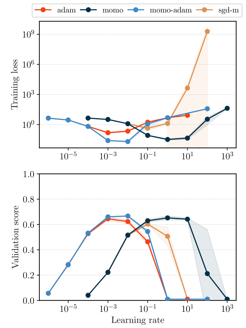
(a) ResNet110 for CIFAR100

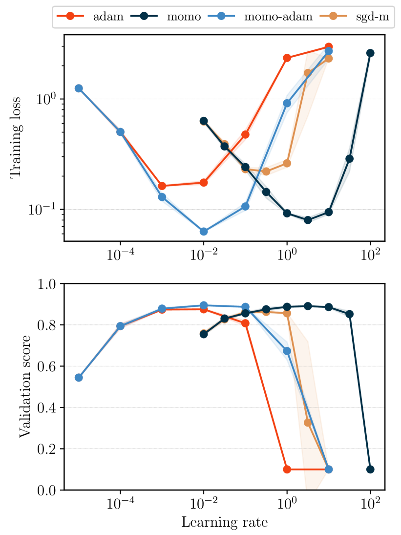
(b) ResNet20 for CIFAR10

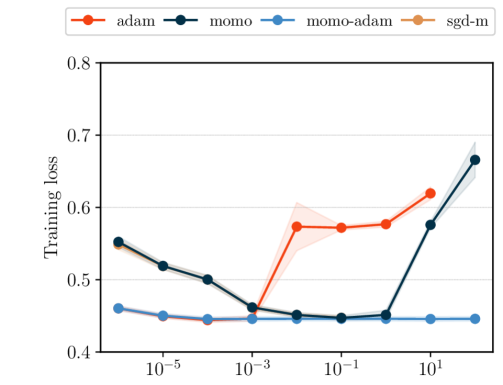
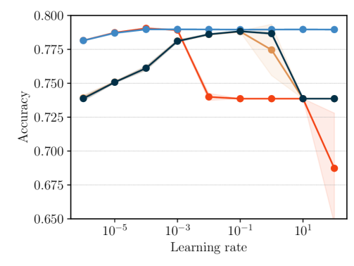
(c) DLRM for Criteo

Figure 2: Training loss (top row) and validation accuracy (bottom row) after a fixed number of epochs, for varying (constant) learning rate $\alpha_{0}$. Shaded area depicts two standard deviations.

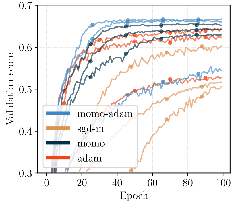
(a) ResNet110 for CIFAR100

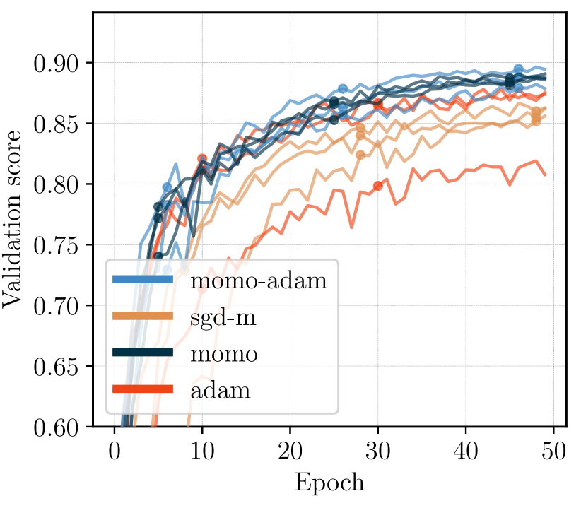
(b) ResNet20 for CIFAR10

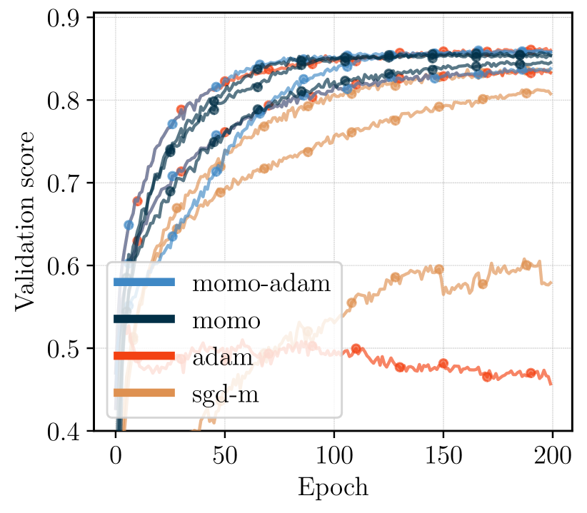
(c) ViT for CIFAR10

Figure 3: Validation score over training, we plot, for each method, the three choices of $\alpha_{0}$ that lead to the best validation score (compare to Fig. 2).

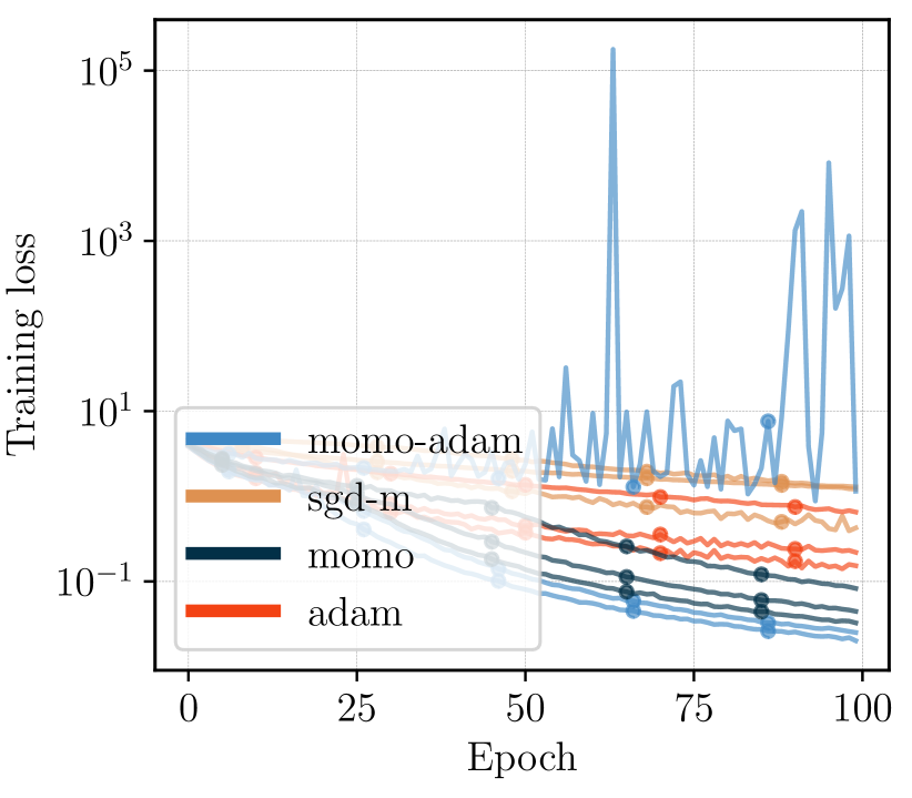
(a) ResNet110 for CIFAR100

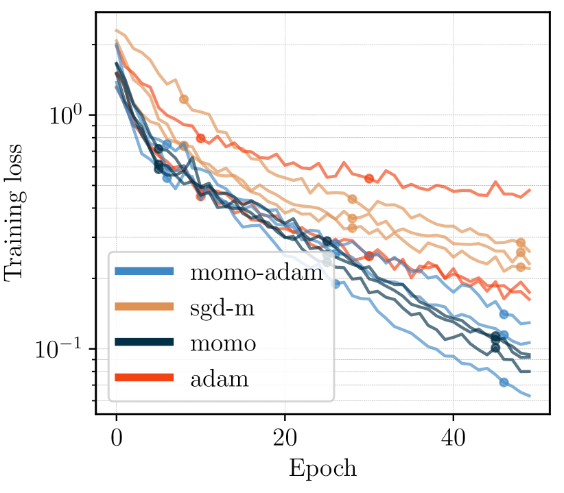
(b) ResNet20 for CIFAR10

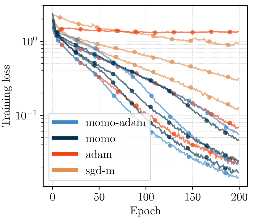
(c) ViT for CIFAR10

Figure 4: Training loss over training, we plot, for each method, the three choices of $\alpha_{0}$ that lead to the best validation score.

5.2 Online Lower Bound Estimation

We now consider image classification on Imagenet32/-1k and a transformer for German-to-English translation. For both problems, the optimal value $f^{*}$ is far away from zero and hence we use MoMo with a known estimate of $f^{*}$ or with the online estimation developed in Section 4. Details on models and datasets are listed in Section E.3.

Imagenet Classification.

We train a ResNet18 for Imagenet32 and give the resulting validation accuracy in Fig. 5(a) for weight decay $\lambda=0$. We show the results $\lambda=10^{-4}$ and for Imagenet-1k in the appendix in Fig. E.3. We run MoMo(-Adam) first with constant lower bound $f_{*}^{k}=0$ and an oracle value $f_{*}^{k}=0.9$. Further, we run MoMo(-Adam)^∗ (indicated by the suffix -star in the plots), (cf. Algorithm 6). We compare to SGD-M and AdamW as baseline. For all methods, we use a constant learning rate $\alpha_{k}=\alpha_{0}$ and vary the value of $\alpha_{0}$.

First, observe that lower bound $f_{*}^{k}=0$ leads to similar performance as the baseline method (in particular it is never worse). Next, observe that the tighter lower bound $f_{*}^{k}=0.9$ leads to improvement for all learning rates. Finally, the online estimated lower bound widens the range of learning rate with good accuracy by an order of magnitude and leads to small improvements in top accuracy.

Transformer for German-to-English Translation.

We consider the task of neural machine translation from German to English by training an encoder-decoder transformer architecture (Vaswani et al., 2017) on the IWSLT14 dataset. We run two settings, namely dropout of $0.1$ and $0.3$. We fine-tune the hyperparameters of the baseline AdamW: for the learning-rate schedule $\alpha_{k}$, we use a linear warm-up of 4000 iterations from zero to a given value $\alpha_{0}$ followed by an inverse square-root decay (cf. Fig. 5(b) for an example curve and the adaptive step sizes). All other parameter settings are given in Section E.3. MoMo-Adam^∗ uses the same hyperparameter settings as AdamW.

Fig. 5(b) shows the BLEU score after 60 epochs when varying the initial learning rate $\alpha_{0}$: MoMo-Adam^∗ is on par or better than AdamW on the full range of initial learning rates and for both dropout values. While the improvement is not as substantial as for previous examples, we remark that for this particular task we compare to a fine-tuned configuration of AdamW.

(a) ResNet18 for Imagenet32

(b) Encoder-Decoder Transformer for IWSLT14

Figure 5: Validation accuracy over a range of learning rates $\alpha_{0}$. (a) Imagenet32 without weight decay ($\lambda=0$). (b) Left: IWSLT14 translation task with dropout 0.1 (plain) or 0.3 (dashed). Right: Learning rate schedule (black) and adaptive step sizes (grey dots) of MoMo-Adam^∗ for $\alpha_{0}=10^{-3}$.

6 Conclusion

We present MoMo and MoMo-Adam, adaptive learning rates for SGD-M and Adam. The main conceptual insight is that momentum can be used to build a model of the loss by averaging a stream of loss function values and gradients. Combined with truncating this average at a known lower bound of the loss, we obtain the MoMo algorithms. This technique can be applied potentially to other methods, for example variants of Adam.

We show examples where incorporating MoMo into SGD-M and Adam significantly reduces the sensitivity to learning rate choice. This can be particularly helpful for practitioners who look for good out-of-the-box optimization performance for new tasks.

Appendix A Implementation details

A.1 Notes on the Averaging Coefficients

Lemma A.1.

Let $\beta\in[0,1)$. Let $\rho_{1,1}=1$, and for $k\geq 2$ let

$$\rho_{j,k}=\begin{cases}\beta\rho_{j,k-1},\quad&j\leq k-1,\\ 1-\beta,\quad&j=k.\end{cases}$$

Then, $\sum_{j=1}^{k}\rho_{j,k}=1$ holds for all $k\in\mathbb{N}$. Further, for an arbitrary sequence $(u_{j})_{j\in\mathbb{N}}\subset\mathbb{R}^{m}$, $m\in\mathbb{N}$, consider the weighted sum

$$\bar{u}_{k}:=\sum_{j=1}^{k}\rho_{j,k}u_{j}.$$

Then, if $\bar{u}_{0}:=u_{1}$ it holds $\bar{u}_{k}=(1-\beta)u_{k}+\beta\bar{u}_{k-1}$ for all $k\in\mathbb{N}$.

Proof.

We prove that $\sum_{j=1}^{k}\rho_{j,k}=1$ holds for all $k\in\mathbb{N}$ by induction. For the base case $k=1$, we have $\rho_{1,1}=1$ by definition. Assuming that $\sum_{j=1}^{k-1}\rho_{j,k-1}=1$, we have

$$\sum_{j=1}^{k}\rho_{j,k}=\rho_{k,k}+\sum_{j=1}^{k-1}\rho_{j,k}=1-\beta+\beta\sum_{j=1}^{k-1}\rho_{j,k-1}=1-\beta+\beta=1.$$

Consequently, we have $\bar{u}_{1}=\rho_{11}u_{1}=u_{1}$, and for $k\geq 2$,

$$\bar{u}_{k} =\sum_{j=1}^{k}\rho_{j,k}u_{j}=(1-\beta)u_{k}+\sum_{j=1}^{k-1}\beta\rho_{j,k-1}u_{j}=(1-\beta)u_{k}+\beta\sum_{j=1}^{k-1}\rho_{j,k-1}u_{j}$$

$$=(1-\beta)u_{k}+\beta\bar{u}_{k-1}.$$

∎

For the choice of $\rho_{j,k}$ in Lemma A.1, unrolling the recursion, for $k\geq 2$ we obtain the explicit formula

$$\rho_{j,k}=\begin{cases}(1-\beta)\beta^{k-j},~{}&j\geq 2\\ \beta^{k-1},~{}&j=1.\end{cases}$$ (22)

Averaging with Bias Correction.

Chosing $\rho_{j,k}=(1-\beta)\beta^{k-j}$, we have $\rho_{j,k}=\beta\rho_{j,k-1}$, and $\rho_{k,k}=1-\beta$. Hence, we can update $\bar{f}_{k}=(1-\beta)f(x^{k},s_{k})+\beta\bar{f}_{k-1}$ and analogously for $d_{k},\gamma_{k}$. However, this choice does not satisfy $\sum_{j=1}^{k}\rho_{j,k}=1$. Indeed using the geometric series gives

$$\rho_{k}=(1-\beta)\sum_{j=0}^{k-1}\beta^{j}=1-\beta^{k}.$$

This fact motivates scaling by the factor of $1-\beta^{k}$ which was termed debiasing in Adam. This alternative averaging scheme leads to a variant of MoMo with bias correction, presented in Algorithm 5. As the two presented choices of $\rho_{j,k}$ are very similar, we do not expect major differences in their performance (cf. Remark A.2).

Input: $x^{1}\in\mathbb{R}^{d}$, $\beta\in[0,\;1)$, $\alpha_{k}>0$, $(f_{*}^{k})_{k\in\mathbb{N}}\subset\mathbb{R}$.

3 Initialize: $\bar{f}_{0}=0,d_{0}=0$ and $\gamma_{0}=0$.

4for $k=1$ to $K-1$ do

5       $\displaystyle\bar{f}_{k}\;=(1-\beta)f(x^{k},s_{k})+\beta\bar{f}_{k-1}$

6      $\displaystyle d_{k}\;=(1-\beta)\nabla f(x^{k},s_{k})+\beta d_{k-1}$

7      $\displaystyle\gamma_{k}=(1-\beta)\left<\nabla f(x^{k},s_{k}),x^{k}\right>+\beta\gamma_{k-1}$

8      $\displaystyle x^{k+1}=x^{k}-\min\Big{\{}\frac{\alpha_{k}}{1-\beta^{k}},\frac{(\bar{f}_{k}-(1-\beta^{k})f_{*}^{k}+\left<d_{k},x^{k}\right>-\gamma_{k})_{+}}{\|d_{k}\|^{2}}\Big{\}}d_{k}.$

Output: $x^{K}$

Defaults settings $\beta=0.9$.

Algorithm 5 MoMo-Bias: Model-based Momentum with bias correction.

Defaults settings $\beta=0.9$.

Remark A.2.

Algorithm 5 differs from Algorithm 1 only in two steps: first, the quantities $\bar{f}_{0},~{}d_{0},~{}\gamma_{0}$ are initialized at zero. Secondly, we use $\frac{\alpha_{k}}{1-\beta^{k}}$ instead of $\alpha_{k}$ and $(1-\beta^{k})f_{*}^{k}$ instead of $f_{*}^{k}$ in line (5). As $\beta\in[0,1)$, for late iteration number $k$, we can expect that both methods behave very similarly.

A.2 Comparison of MoMo-Adam to AdamW

Algorithm 2 naturally compares to AdamW [Loshchilov and Hutter, 2019]. Note that the update of AdamW (in the notation of Algorithm 2) can be written as

$$x^{k+1}=(1-\alpha_{k}\lambda)x^{k}-\frac{\alpha_{k}}{1-\beta_{1}^{k}}{\bf D}_{k}^{-1}d_{k},$$

Compared to Algorithm 2, Algorithm 2, the weight decay of AdamW is not done dividing the whole expression by $\frac{1}{1+\alpha_{k}\lambda}$, but instead multiplying only $x^{k}$ with $1-\alpha_{k}\lambda$. This is a first-order Taylor approximation [Zhuang et al., 2022]: for $\alpha$ small it holds $\frac{1}{1+\alpha\lambda}\approx 1-\alpha\lambda$ and $\frac{\alpha}{1+\alpha\lambda}\approx\alpha$. If we would want to adapt this approximation, we could replace Algorithm 2 with

$$x^{k+1}=(1-\lambda\alpha_{k})x^{k}-\min\Big{\{}\frac{\alpha_{k}}{1-\beta_{1}^{k}},\frac{\big{(}(1+\lambda\alpha_{k})(\bar{f}_{k}-(1-\beta_{1}^{k})f_{*}^{k}-\gamma_{k})+\left<d_{k},x^{k}\right>\big{)}_{+}}{\|d_{k}\|_{{\bf D}_{k}^{-1}}^{2}}\Big{\}}{\bf D}_{k}^{-1}d_{k}.$$ (23)

However, the results of [Zhuang et al., 2022] suggest that this approximation has almost no impact on the empirical performance.

A.3 MoMo^∗

Here we give the complete pseudocode for MoMo^∗, that is the MoMo method that uses the estimator for $f_{*}^{k}$ given in Lemma 4.2.

Input: $x^{1}\in\mathbb{R}^{d}$, $\beta\in[0,\;1)$, $\alpha_{k}>0,f_{*}^{1}\subset\mathbb{R}$.

1 Initialize: $\bar{f}_{0}=f(x^{1},s_{1}),d_{0}=\nabla f(x^{1},s_{1})$ and $\gamma_{0}=\left<d_{0},x^{1}\right>$

2for $k=1$ to $K-1$ do

3       $\displaystyle\bar{f}_{k}\;=(1-\beta)f(x^{k},s_{k})+\beta\bar{f}_{k-1}$

4      $\gamma_{k}=(1-\beta)\left<\nabla f(x^{k},s_{k}),x^{k}\right>+\beta\gamma_{k-1}$

5      $\displaystyle d_{k}\;=(1-\beta)\nabla f(x^{k},s_{k})+\beta d_{k-1}$

6      $\displaystyle f_{*}^{k}=\texttt{ResetStar}()$

7      $\displaystyle x^{k+1}=x^{k}-\min\Big{\{}\alpha_{k},\frac{(\bar{f}_{k}-f_{*}^{k}+\left<d_{k},x^{k}\right>-\gamma_{k})_{+}}{\|d_{k}\|^{2}}\Big{\}}d_{k}$

8      $\displaystyle f_{*}^{k+1}=\texttt{EstimateStar}().$

Output: $x^{K}$

Algorithm 6 MoMo^∗: Adaptive learning rates and online estimation of $f^{*}$.

Appendix B Auxiliary Lemmas

Lemma B.1.

Let $y_{0},a\in\mathbb{R}^{p}$ with $a\neq 0$ and $c\in\mathbb{R}$. Let $\beta>0$. The solution to

$$y^{+}=\arg\min_{y}\underbracket{\Big{(}c+\langle a,y-y_{0}\rangle\Big{)}_{+}}_{=:h(y)}+\frac{1}{2\beta}\|y-y_{0}\|^{2}$$ (24)

is given by

$$y^{+}=y_{0}-\underbracket{\min\big{\{}\beta,\frac{(c)_{+}}{\|a\|^{2}}\big{\}}}_{=:\tau}a.$$

Moreover we have $h(y^{+})=\big{(}c-\tau\|a\|^{2}\big{)}_{+}$ and

$$h(y^{+})=c-\tau\|a\|^{2},\quad \text{if }c\geq 0.$$ (25)

Proof.

Clearly, the objective of (24) is strongly convex and therefore there exists a unique solution. The (necessary and sufficient) first-order optimality condition is given by

$$0=ta+\beta^{-1}(y^{+}-y_{0}),\quad t\in\partial(\cdot)_{+}(c+\langle a,y^{+}-y_{0}\rangle).$$ (26)

We distinguish three cases:

1. Suppose $c<0$. Then, $y_{0}$ satisfies (26) with $t=0$ and hence $y^{+}=y_{0}$. In this case $\tau=0$ and $h(y^{+})=0=(c)_{+}$.

2. Let $\bar{y}:=y_{0}-\beta a$ and assume $c+\langle a,\bar{y}-y_{0}\rangle>0\iff c-\beta\|a\|^{2}>0\iff\frac{c}{\|a\|^{2}}>\beta$. Then $\bar{y}$ satisfies (26) with $t=1$ and hence $y^{+}=\bar{y}$. As $\beta>0$, hence $c>0$ and $\tau=\beta$. As $h(y^{+})=c+\langle a,y^{+}-y_{0}\rangle=c-\beta\|a\|^{2}$, equation (25) holds.

3. If neither $c<0$ nor $\frac{c}{\|a\|^{2}}>\beta$ hold, then it must hold $c+\langle a,y^{+}-y_{0}\rangle=0$. Then, the optimality condition is $0=ta+\beta^{-1}(y^{+}-y_{0})$ for some $t\in[0,1]$. Hence, $y^{+}=y_{0}-t\beta a$ and $c+\langle a,y^{+}-y_{0}\rangle=c-t\beta\|a\|^{2}=0\iff t=\frac{c}{\beta\|a\|^{2}}$. As $c\geq 0$ we have $t\geq 0$ and $\frac{c}{\|a\|^{2}}\leq\beta$ implies $t\leq 1$. Hence, $\tau=\frac{c}{\|a\|^{2}}$ and $c-\tau\|a\|^{2}=c-c=0$, so (25) holds.

∎

Lemma B.2.

Let $y_{0},~{}a\in\mathbb{R}^{p}$ with $a\neq 0$ and $c\in\mathbb{R}$. Let $\mathbf{D}\in\mathbb{R}^{p\times p}$ be a symmetric, positive definite matrix. The solution to

$$y^{+}=\underset{y\in\mathbb{R}^{p}}{\operatorname{argmin}}\;\underbracket{\Big{(}c+\langle a,y-y_{0}\rangle\Big{)}_{+}}_{=:h(y)}+~{}\frac{1}{2\alpha}\|y-y_{0}\|_{\mathbf{D}}^{2}+\frac{\lambda}{2}\|y\|_{\mathbf{D}}^{2}$$ (27)

is given by

$$y^{+}=\frac{1}{1+\lambda\alpha}\Bigg{[}y_{0}-\underbracket{\min\Big{\{}\alpha,\frac{\big{(}(1+\lambda\alpha)c-\lambda\alpha\left<a,y_{0}\right>\big{)}_{+}}{\|a\|_{\mathbf{D}^{-1}}^{2}}\Big{\}}}_{=:\tau}\mathbf{D}^{-1}a\Bigg{]}.$$

Furthermore

$$h(y^{+})=\Big{(}c-\frac{\lambda\alpha}{1+\lambda\alpha}\langle a,y_{0}\rangle-\frac{\tau}{1+\lambda\alpha}\left\|a\right\|_{\mathbf{D}^{-1}}^{2}\Big{)}_{+}.$$

Proof.

First we complete the squares as follows

$$\frac{\lambda}{2}\|y\|_{\mathbf{D}}^{2}+\frac{1}{2\alpha}\|y-y_{0}\|_{\mathbf{D}}^{2} =\frac{1}{2\alpha}\|y\|^{2}_{(1+\lambda\alpha)\mathbf{D}}-\frac{1}{\alpha}\langle y,\mathbf{D}y_{0}\rangle+\mathrm{cst}.(y)$$

$$=\frac{1}{2\alpha}\|y\|^{2}_{(1+\lambda\alpha)\mathbf{D}}-\frac{1}{\alpha}\langle y,(1+\lambda\alpha)\mathbf{D}\tfrac{y_{0}}{1+\lambda\alpha}\rangle+\mathrm{cst}.(y)$$

$$=\frac{1}{2\alpha}\|y-\tfrac{1}{1+\lambda\alpha}y_{0}\|^{2}_{(1+\lambda\alpha)\mathbf{D}}+\mathrm{cst}.(y),$$

where $\mathrm{cst}.(y)$ denotes terms that are constant in $y$. Using the above, (27) is equivalent to

$$y^{+} =\underset{y\in\mathbb{R}^{p}}{\operatorname{argmin}}\;h(y)+\frac{1}{2\alpha}\|y-\tfrac{1}{1+\lambda\alpha}y_{0}\|_{(1+\lambda\alpha)\mathbf{D}}^{2}$$

$$=\underset{y\in\mathbb{R}^{p}}{\operatorname{argmin}}\;\left(c+\langle a,y-\tfrac{1}{1+\lambda\alpha}y_{0}\rangle+\left(\tfrac{1}{1+\lambda\alpha}-1\right)\left<a,y_{0}\right>\right)_{+}+\frac{1}{2\alpha}\|y-\tfrac{1}{1+\lambda\alpha}y_{0}\|_{(1+\lambda\alpha)\mathbf{D}}^{2}.$$

Let $\hat{c}:=c+\left(\tfrac{1}{1+\lambda\alpha}-1\right)\left<a,y_{0}\right>=c-\tfrac{\lambda\alpha}{1+\lambda\alpha}\left<a,y_{0}\right>.$ With this definition, problem (27) is equivalent to

$$y^{+} =\underset{y\in\mathbb{R}^{p}}{\operatorname{argmin}}\;\left(\hat{c}+\langle a,y-\tfrac{1}{1+\lambda\alpha}y_{0}\rangle\right)_{+}+\frac{1}{2\alpha}\|y-\tfrac{1}{1+\lambda\alpha}y_{0}\|_{(1+\lambda\alpha)\mathbf{D}}^{2}.$$

Changing variables with $z^{+}=\mathbf{D}^{1/2}y^{+}$, $z=\mathbf{D}^{1/2}y$, and $z_{0}=\mathbf{D}^{1/2}y_{0}$ gives

$$z^{+} =\underset{z\in\mathbb{R}^{p}}{\operatorname{argmin}}\;\left(\hat{c}+\langle\mathbf{D}^{-1/2}a,z-\tfrac{1}{1+\lambda\alpha}z_{0}\rangle\right)_{+}+\frac{(1+\lambda\alpha)}{2\alpha}\|z-\tfrac{1}{1+\lambda\alpha}z_{0}\|^{2}.$$

Applying Lemma B.1 with $y_{0}\leftarrow\tfrac{1}{1+\lambda\alpha}z_{0},\;c\leftarrow\hat{c},\;a\leftarrow\mathbf{D}^{-1/2}a,\beta\leftarrow\frac{\alpha}{1+\lambda\alpha}$ gives

$$z^{+}=\frac{1}{1+\lambda\alpha}z_{0}-\min\big{\{}\frac{\alpha}{1+\lambda\alpha},\frac{(\hat{c})_{+}}{\|a\|_{\mathbf{D}^{-1}}^{2}}\big{\}}\mathbf{D}^{-1/2}a.$$

Changing variables back using $y^{+}=\mathbf{D}^{-1/2}z^{+}$, substituting $\hat{c}=c-\tfrac{\lambda\alpha}{1+\lambda\alpha}\left<a,y_{0}\right>$ and re-arranging the above gives

$$y^{+} =\frac{1}{1+\lambda\alpha}y_{0}-\min\Big{\{}\frac{\alpha}{1+\lambda\alpha},\frac{\big{(}c-\tfrac{\lambda\alpha}{1+\lambda\alpha}\left<a,y_{0}\right>\big{)}_{+}}{\|a\|_{\mathbf{D}^{-1}}^{2}}\Big{\}}\mathbf{D}^{-1}a$$

$$=\frac{1}{1+\lambda\alpha}\Bigg{[}y_{0}-\min\Big{\{}\alpha,\frac{\big{(}(1+\lambda\alpha)c-\lambda\alpha\left<a,y_{0}\right>\big{)}_{+}}{\|a\|_{\mathbf{D}^{-1}}^{2}}\Big{\}}\mathbf{D}^{-1}a\Bigg{]}.$$ (28)

∎

Appendix C Missing Proofs

C.1 Proof of Lemma 2.1

See 2.1

Proof.

Recall problem (10) given by

$$x^{k+1}=\underset{y\in\mathbb{R}^{d}}{\operatorname{argmin}}\;m_{k}(y)+\frac{1}{2\alpha_{k}}\|y-x^{k}\|^{2}.$$

Introducing

$$h_{k}\coloneqq\sum_{j=1}^{k}\rho_{j,k}[f(x^{j},s_{j})+\langle\nabla f(x^{j},s_{j}),x^{k}-x^{j}\rangle]=\bar{f}_{k}+\langle d_{k},x^{k}\rangle-\gamma_{k},$$ (29)

we have that

$$m_{k}(y)=\max\Big{\{}\rho_{k}^{-1}(h_{k}+\langle d_{k},y-x^{k}\rangle),f_{*}^{k}\Big{\}}=\Big{(}\rho_{k}^{-1}(h_{k}+\langle d_{k},y-x^{k}\rangle)-f_{*}^{k}\Big{)}_{+}+f_{*}^{k}.$$ (30)

Using (30), dropping the constant term $f_{*}^{k}$, and multiplying with $\rho_{k}$, problem (10) is equivalent to

$$x^{k+1}=\underset{y\in\mathbb{R}^{d}}{\operatorname{argmin}}\;\Big{(}h_{k}+\langle d_{k},y-x^{k}\rangle-\rho_{k}f_{*}^{k}\Big{)}_{+}+\frac{\rho_{k}}{2\alpha_{k}}\|y-x^{k}\|^{2}.$$

Applying Lemma B.1 with $\beta\leftarrow\rho_{k}^{-1}\alpha_{k}$, $c\leftarrow h_{k}-\rho_{k}f_{*}^{k}$, $a\leftarrow d_{k}$ and $y_{0}\leftarrow x^{k}$ gives the result. ∎

C.2 Proof of Lemma 3.1

See 3.1

Proof.

Recall problem (14) given by

$$x^{k+1}=\underset{y\in\mathbb{R}^{d}}{\operatorname{argmin}}\;m_{k}(y)+\frac{1}{2\alpha_{k}}\|y-x^{k}\|_{{\bf D}_{k}}^{2}+\frac{\lambda}{2}\|y\|_{{\bf D}_{k}}^{2}.$$

We use again (30). Dropping the constant term $f_{*}^{k}$, and multiplying with $\rho_{k}$, problem (14) is equivalent to

$$x^{k+1}=\underset{y\in\mathbb{R}^{d}}{\operatorname{argmin}}\;\Big{(}h_{k}+\langle d_{k},y-x^{k}\rangle-\rho_{k}f_{*}^{k}\Big{)}_{+}+\frac{\rho_{k}}{2\alpha_{k}}\|y-x^{k}\|_{{\bf D}_{k}}^{2}+\frac{\rho_{k}\lambda}{2}\|y\|_{{\bf D}_{k}}^{2}.$$

Now applying Lemma B.2 with $y_{0}\leftarrow x^{k}$, $a\leftarrow d_{k}$, $c\leftarrow h_{k}-\rho_{k}f_{*}^{k}$, $\lambda\leftarrow\rho_{k}\lambda$, $\alpha\leftarrow\rho_{k}^{-1}\alpha_{k}$ and $\mathbf{D}\leftarrow{\bf D}_{k}$, we obtain the result. ∎

Appendix D Estimating a Lower Bound: Proofs and Alternatives

D.1 Proof of Lemma 4.2

See 4.2

Proof.

Consider the update (16) without weight decay, that is $\lambda=0$, and switching the index $k\to j$, which is

$$x^{j+1}=x^{j}-\tau_{j}{\bf D}_{j}^{-1}d_{j},$$

where $\tau_{j}$ is the step size. Subtracting $x^{*}$ from both sides, taking norms and expanding the squares we have that

$$\left\|x^{j+1}-x^{*}\right\|_{{\bf D}_{j}}^{2} =\left\|x^{j}-x^{*}\right\|_{{\bf D}_{j}}^{2}-2\tau_{j}\left<d_{j},x^{j}-x^{*}\right>+\tau_{j}^{2}\left\|d_{j}\right\|_{{\bf D}_{j}^{-1}}^{2}.$$ (31)

Now let $\delta_{j+1}:=\lambda_{\min}\big{(}{\bf D}_{j+1}^{-1}{\bf D}_{j}\big{)}$ and note that for every vector $v\in\mathbb{R}^{d}$ we have that

$$\delta_{j+1}\left\|v\right\|^{2}_{{\bf D}_{j+1}}\leq\left\|v\right\|^{2}_{{\bf D}_{j}}.$$ (32)

Indeed this follows since

$$\left\|v\right\|^{2}_{{\bf D}_{j}} =v^{\top}{\bf D}_{j}v=v^{\top}{\bf D}_{j+1}^{1/2}\big{(}{\bf D}_{j+1}^{-1/2}{\bf D}_{j}{\bf D}_{j+1}^{-1/2}\big{)}{\bf D}_{j+1}^{1/2}v$$

$$\geq\lambda_{\min}\big{(}{\bf D}_{j+1}^{-1}{\bf D}_{j}\big{)}\left\|v\right\|_{{\bf D}_{j+1}}^{2}=\delta_{j+1}\left\|v\right\|_{{\bf D}_{j+1}}^{2}.$$

For simplicity, denote $\nabla f_{l}=\nabla f(x^{l},s_{l}),f_{l}=f(x^{l},s_{l})$. We have that

$$\left<d_{j},x^{j}-x^{*}\right> =\sum_{l=1}^{j}\rho_{l,j}\left<\nabla f_{l},x^{j}-x^{*}\right>$$

$$=\sum_{l=1}^{j}\rho_{l,j}\left(\left<\nabla f_{l},x^{j}-x^{l}\right>+\left<\nabla f_{l},x^{l}-x^{*}\right>\right)$$

$$\geq\sum_{l=1}^{j}\rho_{l,j}\left(\left<\nabla f_{l},x^{j}-x^{l}\right>+f_{l}-f(x^{*},s_{l})\right) f(\cdot,s)$$ (by convexity of )

$$=\bar{f}_{j}+\left<d_{j},x^{j}\right>-\gamma_{j}-\sum_{l=1}^{j}\rho_{l,j}f(x^{*},s_{l})\;=\;h_{j}-\rho_{j}\bar{f}_{*}^{j}.$$ (33)

Using (32) together with (33) in (31) gives

$$\delta_{j+1}\left\|x^{j+1}-x^{*}\right\|_{{\bf D}_{j+1}}^{2} \leq\left\|x^{j+1}-x^{*}\right\|_{{\bf D}_{j}}^{2}$$

$$=\left\|x^{j}-x^{*}\right\|_{{\bf D}_{j}}^{2}-2\tau_{j}\left<d_{j},x^{j}-x^{*}\right>+\tau_{j}^{2}\left\|d_{j}\right\|_{{\bf D}_{j}^{-1}}^{2}$$

$$\leq\left\|x^{j}-x^{*}\right\|_{{\bf D}_{j}}^{2}-2\tau_{j}(h_{j}-\rho_{j}\bar{f}_{*}^{j})+\tau_{j}^{2}\left\|d_{j}\right\|_{{\bf D}_{j}^{-1}}^{2}.$$ (34)

Now we will perform a weighted telescoping. We will multiply the above by $\eta_{j}>0$ such that $\delta_{j+1}\eta_{j}=\eta_{j+1},$ thus $\eta_{j}=\eta_{1}\prod_{l=2}^{j}\delta_{l}.$ Thus multiplying through by $\eta_{j}$ we have that

$$\eta_{j+1}\left\|x^{j+1}-x^{*}\right\|_{{\bf D}_{j+1}}^{2} \leq\eta_{j}\left\|x^{j}-x^{*}\right\|_{{\bf D}_{j}}^{2}-2\eta_{j}\tau_{j}(h_{j}-\rho_{j}\bar{f}_{*}^{j})+\eta_{j}\tau_{j}^{2}\left\|d_{j}\right\|_{{\bf D}_{j}^{-1}}^{2}.$$

Summing up from $j=1,\ldots,k$ and telescoping we have that

$$0 \leq\eta_{k+1}\left\|x^{k+1}-x^{*}\right\|_{{\bf D}_{k+1}}^{2}$$

$$\leq\eta_{1}\left\|x^{1}-x^{*}\right\|_{{\bf D}_{1}}^{2}-2\sum_{j=1}^{k}\eta_{j}\tau_{j}(h_{j}-\rho_{j}\bar{f}_{*}^{j})+\sum_{j=1}^{k}\eta_{j}\tau_{j}^{2}\left\|d_{j}\right\|_{{\bf D}_{j}^{-1}}^{2}.$$ (35)

Re-arranging the above, choosing $\eta_{1}=1$ and isolating $\bar{f}_{*}^{k}$ gives

$$2\eta_{k}\tau_{k}\rho_{k}\bar{f}_{*}^{k} \geq 2\sum_{j=1}^{k}\eta_{j}\tau_{j}h_{j}-\left\|x^{1}-x^{*}\right\|_{{\bf D}_{1}}^{2}-\sum_{j=1}^{k}\eta_{j}\tau_{j}^{2}\left\|d_{j}\right\|_{{\bf D}_{j}^{-1}}^{2}-2\sum_{j=1}^{k-1}\eta_{j}\tau_{j}\rho_{j}\bar{f}_{*}^{j}.$$

Dividing through by $2\eta_{k}\tau_{k}\rho_{k}$ gives the main result. Finally the recurrence follows since, for $k\geq 2$ we have that

$$f_{*}^{k+1}=\frac{2\sum_{j=1}^{k}\eta_{j}\tau_{j}h_{j}-\left\|x^{1}-x^{*}\right\|_{{\bf D}_{1}}^{2}-\sum_{j=1}^{k}\eta_{j}\tau_{j}^{2}\left\|d_{j}\right\|_{{\bf D}_{j}^{-1}}^{2}-2\sum_{j=1}^{k-1}\eta_{j}\tau_{j}\rho_{j}\bar{f}_{*}^{j}}{2\eta_{k}\tau_{k}\rho_{k}}$$

$$=\frac{\eta_{k-1}\tau_{k-1}\rho_{k-1}}{\eta_{k}\tau_{k}\rho_{k}}\underbracket{\frac{2\sum_{j=1}^{k-1}\eta_{j}\tau_{j}h_{j}-\left\|x^{1}-x^{*}\right\|_{{\bf D}_{1}}^{2}-\sum_{j=1}^{k-1}\eta_{j}\tau_{j}^{2}\left\|d_{j}\right\|_{{\bf D}_{j}^{-1}}^{2}-2\sum_{j=1}^{k-2}\eta_{j}\tau_{j}\rho_{j}\bar{f}_{*}^{j}}{2\eta_{k-1}\tau_{k-1}\rho_{k-1}}}_{=f_{*}^{k}}$$

$$\hskip 8.61108pt\;+\frac{\eta_{k-1}\tau_{k-1}\rho_{k-1}}{\eta_{k}\tau_{k}\rho_{k}}\frac{2\eta_{k}\tau_{k}h_{k}-\eta_{k}\tau_{k}^{2}\left\|d_{k}\right\|_{{\bf D}_{k}^{-1}}^{2}-2\eta_{k-1}\tau_{k-1}\rho_{k-1}\bar{f}_{*}^{k-1}}{2\eta_{k-1}\tau_{k-1}\rho_{k-1}}$$

$$=\frac{2\eta_{k-1}\tau_{k-1}\rho_{k-1}(f_{*}^{k}-\bar{f}_{*}^{k-1})-\eta_{k}\tau_{k}^{2}\left\|d_{k}\right\|_{{\bf D}_{k}^{-1}}^{2}+2\eta_{k}\tau_{k}h_{k}}{2\eta_{k}\tau_{k}\rho_{k}}.$$

Now bootstrapping by using $f_{*}^{k}\approx\bar{f}_{*}^{k-1}$ gives the result. ∎

D.2 The Max Lower Bound

Here we derive an alternative estimate for the lower bound that does not require bootstrapping, contrary to Lemma 4.2.

Lemma D.1.

Let $f(x,s)$ be convex in $x$ for every sample $s$. Furthermore let $x^{*}\in\underset{x\in\mathbb{R}^{d}}{\operatorname{argmin}}\;f(x)$. Consider $x^{k}$ are the iterates of (16) with $\lambda=0$ and let

$$\eta_{k}=\prod_{j=2}^{k}\lambda_{\min}\big{(}{\bf D}_{j}^{-1}{\bf D}_{j-1}\big{)},\;\bar{f}_{*}^{k}:=\frac{1}{\rho_{k}}\sum_{j=1}^{k}\rho_{j,k}f(x^{*},s_{j}),\;h_{k}=\bar{f}_{k}+\langle d_{k},x^{k}\rangle-\gamma_{k}.$$

It follows that

$$\max_{j=1,\ldots,k}\bar{f}_{*}^{j}\geq f_{*}^{k+1}\coloneqq\frac{2\sum_{j=1}^{k}\eta_{j}\tau_{j}h_{j}-\left\|x^{1}-x^{*}\right\|^{2}-\sum_{j=1}^{k}\eta_{j}\tau_{j}^{2}\left\|d_{j}\right\|_{{\bf D}_{j}^{-1}}^{2}}{2\sum_{j=1}^{k}\eta_{j}\tau_{j}\rho_{j}}.$$ (36)

Furthermore we have the recurrence

$$f_{*}^{k+1} =\;\frac{f_{*}^{k}\sum_{j=1}^{k-1}\eta_{j}\tau_{j}\rho_{j}+\eta_{k}\tau_{k}\left(h_{k}-\frac{1}{2}\tau_{k}\left\|d_{k}\right\|_{{\bf D}_{k}^{-1}}^{2}\right)}{\sum_{j=1}^{k}\eta_{j}\tau_{j}\rho_{j}}.$$ (37)

In particular when ${\bf D}_{k}=\mathbf{Id}$ for every $k$, then we have that $\eta_{k}=1$ for all $k$.

Proof.

From step (35) and re-arranging we have that

$$2\big{(}\max_{j=1,\ldots,k}\bar{f}_{*}^{j}\big{)}\big{(}\sum_{j=1}^{k}\eta_{j}\tau_{j}\rho_{j}\big{)}\; \geq 2\big{(}\sum_{j=1}^{k}\eta_{j}\tau_{j}\rho_{j}\big{)}\bar{f}_{*}^{j}$$

$$\geq 2\sum_{j=1}^{k}\eta_{j}\tau_{j}h_{j}-\left\|x^{1}-x^{*}\right\|_{{\bf D}_{1}}^{2}-\sum_{j=1}^{k}\eta_{j}\tau_{j}^{2}\left\|d_{j}\right\|_{{\bf D}_{j}^{-1}}^{2}.$$

If we now assume that $\bar{f}_{*}^{j}\approx f(x^{*})$ (or upper bounding $\bar{f}_{*}^{j}$ by a constant) then by substituting in $f(x^{*})$, dividing through by $\big{(}\sum_{j=1}^{k}\eta_{j}\tau_{j}\rho_{j}\big{)}$ gives the estimate

$$\max_{j=1,\ldots,k}\bar{f}_{*}^{j}\geq f_{*}^{k+1}\coloneqq\frac{2\sum_{j=1}^{k}\eta_{j}\tau_{j}h_{j}-\left\|x^{1}-x^{*}\right\|^{2}-\sum_{j=1}^{k}\eta_{j}\tau_{j}^{2}\left\|d_{j}\right\|_{{\bf D}_{j}^{-1}}^{2}}{2\sum_{j=1}^{k}\eta_{j}\tau_{j}\rho_{j}}.$$

Finally the recurrence follows since

$$f_{*}^{k+1} =\frac{2\sum_{j=1}^{k}\eta_{j}\tau_{j}h_{j}-\left\|x^{1}-x^{*}\right\|_{{\bf D}_{1}}^{2}-\sum_{j=1}^{k}\eta_{j}\tau_{j}^{2}\left\|d_{j}\right\|_{{\bf D}_{j}^{-1}}^{2}}{2\sum_{j=1}^{k}\eta_{j}\tau_{j}\rho_{j}}$$

$$=\frac{\sum_{j=1}^{k-1}\eta_{j}\tau_{j}\rho_{j}}{\sum_{j=1}^{k}\eta_{j}\tau_{j}\rho_{j}}\frac{2\sum_{j=1}^{k-1}\eta_{j}\tau_{j}h_{j}-\left\|x^{1}-x^{*}\right\|_{{\bf D}_{1}}^{2}-\sum_{j=1}^{k-1}\eta_{j}\tau_{j}^{2}\left\|d_{j}\right\|_{{\bf D}_{j}^{-1}}^{2}}{2\sum_{j=1}^{k-1}\eta_{j}\tau_{j}\rho_{j}}$$

$$\quad+\frac{2\eta_{k}\tau_{k}h_{k}-\eta_{k}\tau_{k}^{2}\left\|d_{k}\right\|_{{\bf D}_{k}^{-1}}^{2}}{2\sum_{j=1}^{k}\eta_{j}\tau_{j}\rho_{j}}$$

$$=\frac{f_{*}^{k}\sum_{j=1}^{k-1}\eta_{j}\tau_{j}\rho_{j}+\eta_{k}\tau_{k}\left(h_{k}-\frac{1}{2}\tau_{k}\left\|d_{k}\right\|_{{\bf D}_{k}^{-1}}^{2}\right)}{\sum_{j=1}^{k}\eta_{j}\tau_{j}\rho_{j}}.$$

∎

Appendix E Additional Information on Experiments

E.1 Additional Plots

(a) VGG16 for CIFAR10

(b) ViT for CIFAR10

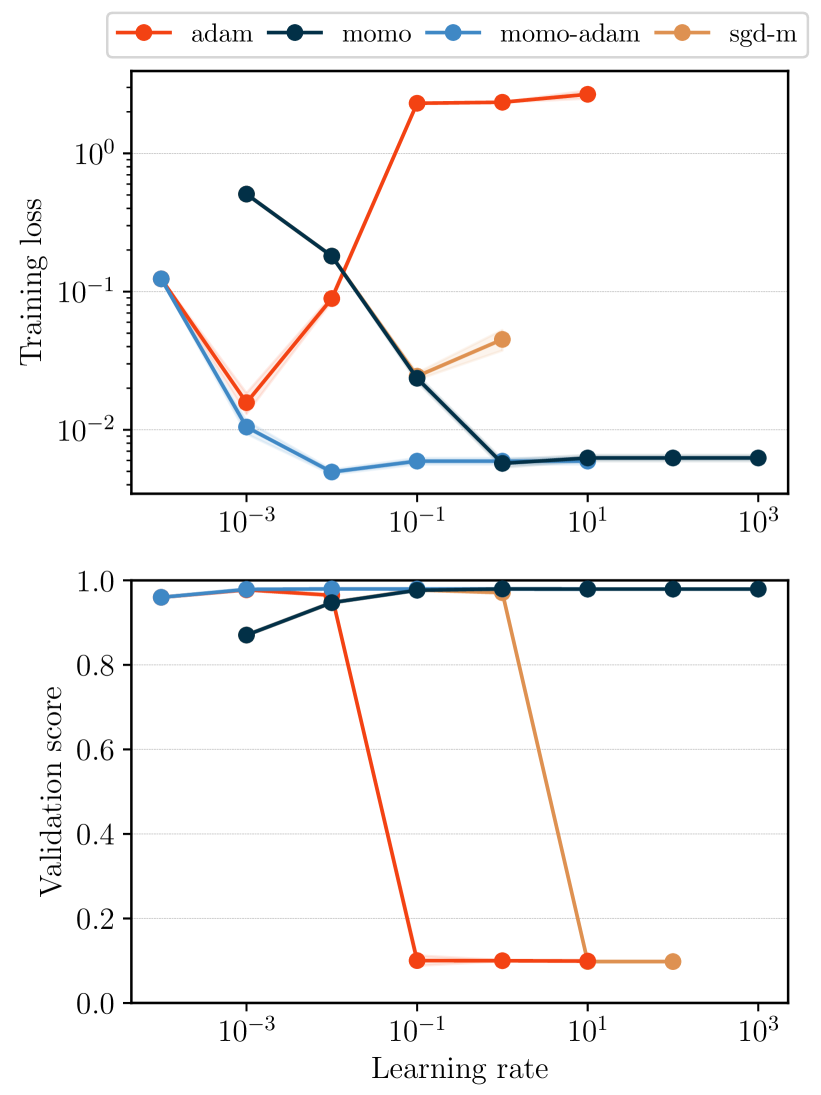
(c) MLP for MNIST

Figure E.1: Training loss (top row) and validation accuracy (bottom row) after a fixed number of epochs, for varying (constant) learning rate $\alpha_{0}$.

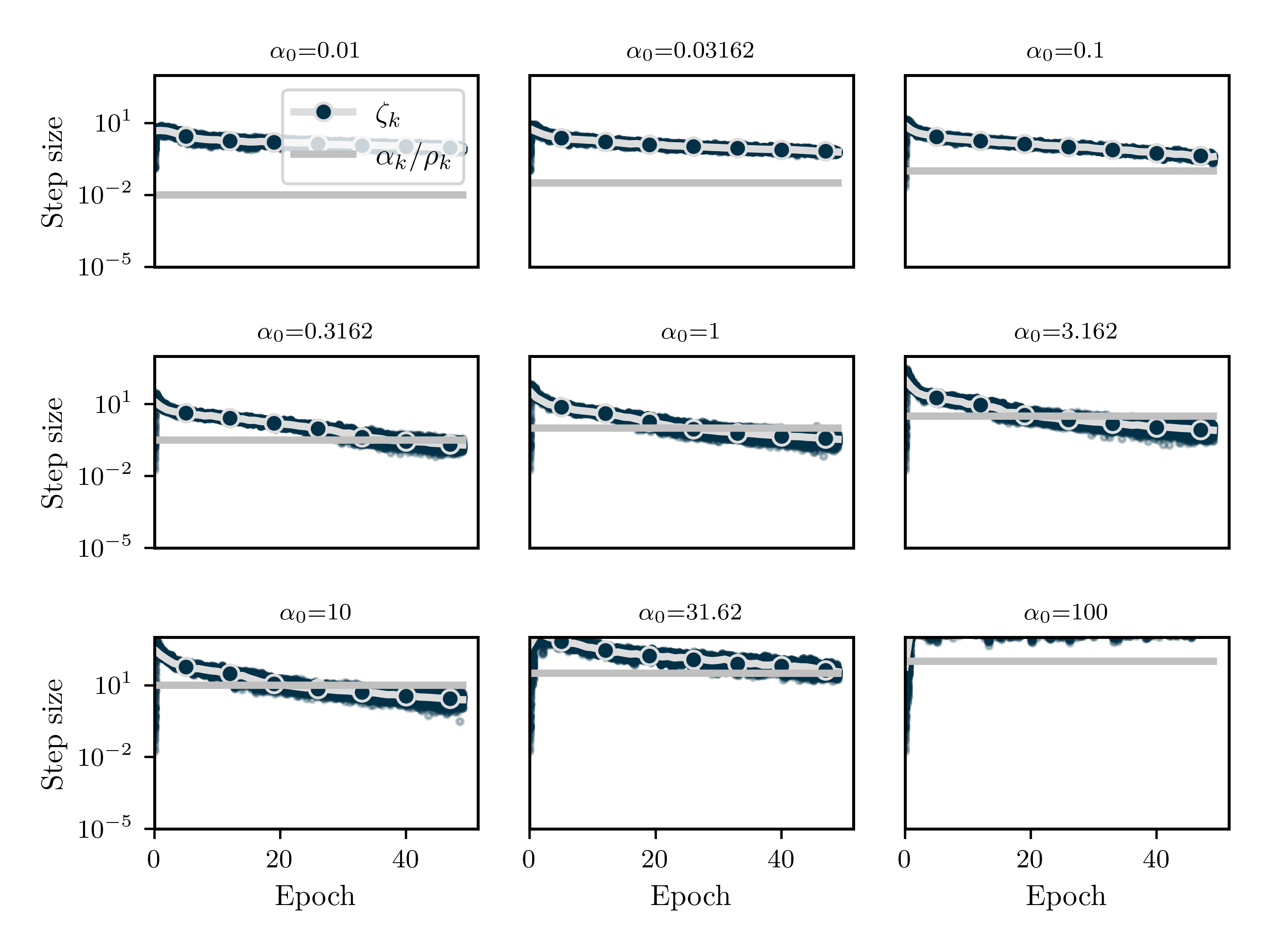
(a) MoMo

(b) MoMo-Adam

Figure E.2: ResNet20 for CIFAR10. Adaptive learning rate of MoMo (left) and MoMo-Adam (right). The colored dots represent the term $\zeta_{k}$ in each iteration. The grey line represents the user-specified learning rate $\alpha_{k}/\rho_{k}$ (note that $\rho_{k}=1$ for MoMo and $\rho_{k}\approx 1$ except for the first few iterations in MoMo-Adam). The minimum of the grey line and the dots is the adaptive learning rate $\tau_{k}=\min\{\frac{\alpha_{k}}{\rho_{k}},\zeta_{k}\}$ in each iteration. The silver line with colored markers is the median over the values of $\zeta_{k}$ in each epoch.

	MoMo	MoMo-Adam	SGD-M	Adam
ResNet110 for CIFAR100	65.21$~{}\pm 1.61$	66.71$~{}\pm 0.31$	60.28$~{}\pm 0.36$	64.5$~{}\pm 1.14$
ResNet20 for CIFAR10	89.07$~{}\pm 0.2$	89.45$~{}\pm 0.17$	86.27$~{}\pm 0.67$	87.54$~{}\pm 0.26$
ViT for CIFAR10	85.43$~{}\pm 0.19$	85.81$~{}\pm 0.57$	83.39$~{}\pm 0.28$	86.02$~{}\pm 0.44$
VGG16 for CIFAR10	90.64$~{}\pm 0.18$	90.9$~{}\pm 0.17$	89.81$~{}\pm 0.43$	89.95$~{}\pm 0.67$
MLP for MNIST	97.97$~{}\pm 0.08$	97.96$~{}\pm 0.12$	97.73$~{}\pm 0.12$	97.75$~{}\pm 0.06$
DLRM for Criteo	78.83 $~{}\pm 0.038$	78.98 $~{}\pm 0.036$	78.81 $~{}\pm 0.041$	79.05 $~{}\pm 0.014$
ResNet18 for Imagenet32	47.66∗	47.54∗	47.38	46.98
ResNet18 for Imagenet-1k	69.68	N/A	69.57	N/A
IWSLT14 (dp 0.1)	N/A	33.63∗	N/A	32.56
IWSLT14 (dp 0.3)	N/A	35.34∗	N/A	34.97

Table 1: Validation score (with one standard deviation) for the best learning rate choice for each method among the ones displayed in Section 5. Symbol “^∗" indicates usage of online lower bound, otherwise MoMo(-Adam) used with $f_{\star}^{k}=0$. Bold indicates the best method (for experiments with multiple seeds, we only mark in bold if the advantage is outside of standard deviation).

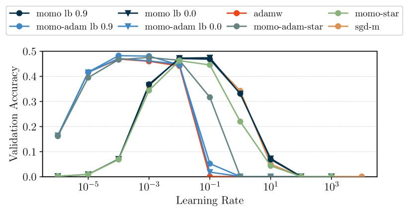
(a) ResNet18 for Imagenet32

(b) ResNet18 for Imagenet-1k

Figure E.3: Left: Validation accuracy of a ResNet18 for Imagenet32 with weight decay $\lambda=10^{-4}$. Right: Validation accuracy of a ResNet18 for Imagenet-1k, with standard exponential learning rate schedule (decay factor 10 at epochs 30 and 60) and constant learning rate schedule.

E.2 Experimental Setup of Section 5.1

We set the momentum parameter $\beta=0.9$ for MoMo and SGD-M, and $(\beta_{1},\beta_{2})=(0.9,0.999)$ for MoMo-Adam and Adam respectively. We do not use weight decay, i.e. $\lambda=0$.

For SGD-M we set the dampening parameter (in Pytorch) equal to the momentum parameter $0.9$. Like this, SGD-M does an exponentially-weighted average of past gradients and hence is comparable to MoMo for identical learning rate and momentum. Setting $\texttt{dampening}=0.9$ is equivalent to running with $\texttt{dampening}=0$ and a ten times smaller learning rate. For all other hyperparameters we use the Pytorch default values for Adam and SGD-M (unless explicitly stated otherwise).

E.3 Models and Datasets

ResNet for CIFAR

[He et al., 2016] 
Used for ResNet20 for CIFAR10 and ResNet110 for CIFAR100. We adapt the last layer output size to $\{10,100\}$ according to the used dataset. We run 50 epochs for ResNet20 and $100$ epochs for ResNet110.

Model

https://github.com/akamaster/pytorch_resnet_cifar10/blob/master/resnet.py

VGG16 for CIFAR10

[Simonyan and Zisserman, 2015] 
A deep network with 16 convolutional layers. We run 50 epochs.

Model

https://github.com/chengyangfu/pytorch-vgg-cifar10/blob/master/vgg.py

ViT for CIFAR10

[Dosovitskiy et al., 2021] 
A small vision transformer, based on the hyperparameter setting proposed in github.com/kentaroy47/vision-transformers-cifar10. In particular, we set the patch size to four. We run 200 epochs.

Model

https://github.com/lucidrains/vit-pytorch

ResNet18 for Imagenet32

[He et al., 2016] 
Imagenet32 is a downsampled version of Imagenet-1k to images of $32\times 32$ pixels. We adapt the last layer output size to $1000$. We run 45 epochs.

Model

https://github.com/kuangliu/pytorch-cifar/blob/master/models/resnet.py

ResNet18 for Imagenet-1k

[He et al., 2016] 
We use both a constant learning rate and a schedule that decays the learning rate by 0.1 every 30 epochs. We run 90 epochs. Note that for SGD-M the decaying schedule with initial learning rate of $0.1$ is considered state-of-the-art. As we set $\texttt{dampening}=0.9$, and this is equivalent to $\texttt{dampening}=0$ and a ten times smaller learning rate (see Section E.2), in our plots the best score is displayed for initial learning rate of $1$ accordingly.

Model

pytorch.org/vision/main/models/generated/torchvision.models.resnet18.html

DLRM for Criteo

[Tien and Chapelle, 2014] 
DLRM is an industry-scale model with over 300 million parameters. the Criteo dataset contains approximately $46$ million training samples. We run 300k iterations with batch size 128.

Dataset	https://kaggle.com/c/criteo-display-ad-challenge
Model	https://github.com/facebookresearch/dlrm

IWSLT14

[Ott et al., 2019] 
We use a transformer with six encoder and decoder blocks from fairseq. The training loss is the cross-entropy loss with label smoothing of $0.1$. We use weight decay of $\lambda=10^{-4}$ (although we noticed that weight decay does not influence the performance of MoMo-Adam), momentum parameters $(\beta_{1},\beta_{2})=(0.9,0.98)$. We train for $60$ epochs.

Model

https://github.com/facebookresearch/fairseq

For each experiments, we list how long one training run approximately takes on the hardware we use. Unless specified otherwise, we train on a single NVIDIA A100 GPU. ResNet110 for CIFAR100 $90$ min, ResNet20 for CIFAR10 $30$ min, VGG16 for CIFAR10 $30$ min, MLP for MNIST $3$ min, ResNet18 for Imagenet32 20 hours (on NVIDIA V100), Transformer for IWSLT14 $3$ hours.

E.4 Illustrative Example of Online Lower Bound Estimation

We show how our online estimation of $f_{*}^{k}$, derived in Section 4 and Lemma 4.2, work for a simple example. Consider a regression problem, with synthetic matrix $A\in\mathbb{R}^{200\times 10}$ and $b\in\mathbb{R}^{200}$. We solve the problem $\min_{x\in\mathbb{R}^{10}}\sum_{i=1}^{200}\frac{1}{2}\|a_{i}^{\top}x-b_{i}\|^{2}$, where $a_{i}$ are the rows of $A$. The data is generated in a way such that there exists $\hat{x}$ with $b=A\hat{x}$ and hence the optimal value is $f^{*}=0$.

We now run MoMo(-Adam) with lower bound estimate $f_{*}^{k}=-10$ in all iterations, and MoMo(-Adam)^∗ with initialization $f_{*}^{1}=-10$. Clearly, this is not a tight estimate of the optimal value $f^{*}$. From Fig. 4(a), we see that online estimation of $f_{*}^{k}$, used in MoMo(-Adam)^∗, improves stability of the training compared to plain MoMo(-Adam) where a constant value $f_{*}^{k}=-10$ is used. From Fig. 4(b), we also see that the online values of $f_{*}^{k}$ converge to $f^{*}=0$.

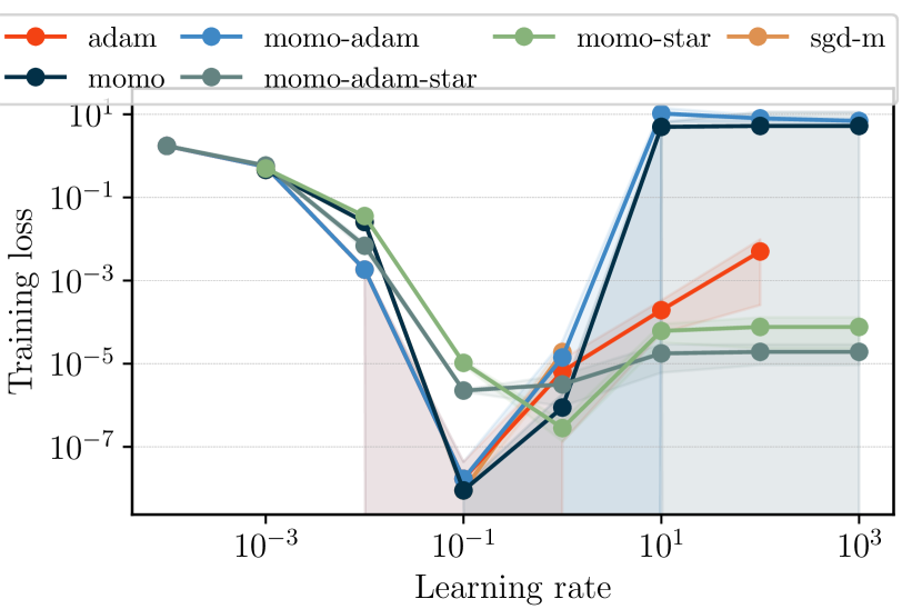
(a) Training Loss

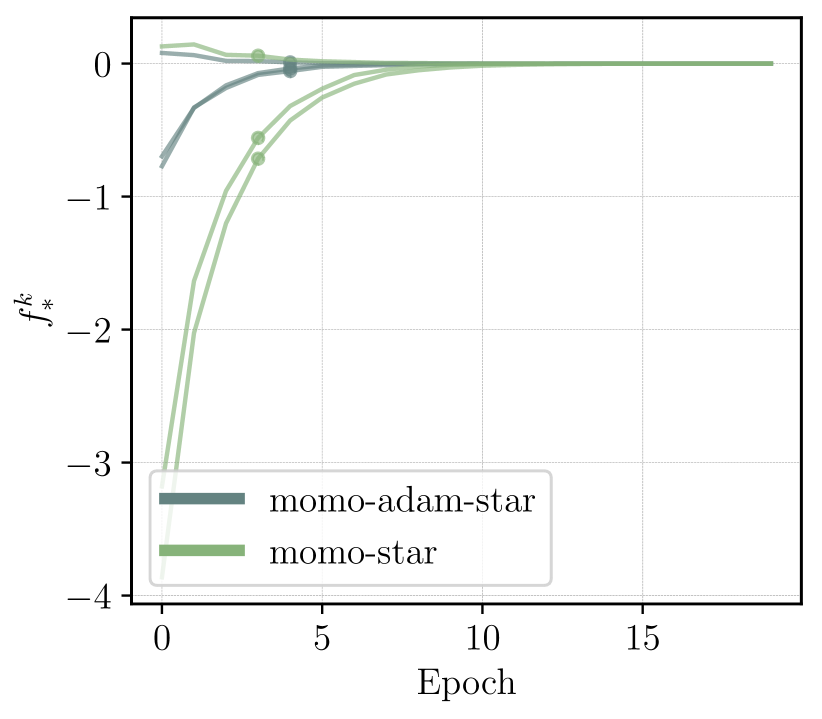
(b) Online estimation of $f^{*}=0$

Figure E.4: Illustrative example of online lower bound estimation. For all MoMo methods, we initialize $f_{*}^{1}=-10$. Left: Training loss for varying (constant) learning rate $\alpha_{0}$. Right: Value of $f_{*}^{k}$ over training, one line corresponds to one choice of $\alpha_{0}$. We plot per method the four values of $\alpha_{0}$ that lead to smallest training loss.

Appendix F Convergence Analysis

Here we give another motivation for a variant of MoMo through convexity. We discovered this interpretation of MoMo after reading the concurrent work [Wang et al., 2023].

For this alternative derivation of MoMo, first let $\tau_{k}\geq 0$ be a free parameter, and consider a general momentum method with a preconditioner given by

$$\begin{split}d_{k}&=\sum_{j=1}^{k}\rho_{j,k}\nabla f(x^{j},s_{j}),\\ x^{k+1}&=x^{k}-\tau_{k}{\bf D}_{k}^{-1}d_{k}.\end{split}$$ (38)

We can now view $x^{k+1}$ as a function of $\tau_{k}$, that is $x^{k+1}(\tau_{k})$. Ideally we would like to choose $\tau_{k}$ so that $x^{k+1}$ is as close as possible to the optimum solution $x^{*}$, that is to minimize $\left\|x^{k+1}(\tau_{k})-x^{*}\right\|_{{\bf D}_{k}}^{2}$ in $\tau_{k}.$ This is general not possible because we do not know $x^{*}.$ But if we assume that $f(\cdot,s)$ is a convex function, then we can minimize an upper bound of $\left\|x^{k+1}(\tau_{k})-x^{*}\right\|_{{\bf D}_{k}}^{2}$ with respect to $\tau_{k}$. As we show next, this gives the adaptive term in the learning rate of MoMo if $f_{*}^{k}=\bar{f}^{k}_{*}$.

Lemma F.1.

Let $f(\cdot,s)$ be convex for every $s$. Let $h_{k}:=\bar{f}_{k}+\langle d_{k},x^{k}\rangle-\gamma_{k}$ where $d_{k},\bar{f}_{k},$ and $\gamma_{k}$ are defined in (11). Consider the iterates given by (38) and let $x^{*}\in\arg\min_{x\in\mathbb{R}^{d}}f(x)$. Then, we have the upper bound

$$\left\|x^{k+1}-x^{*}\right\|_{{\bf D}_{k}}^{2} \leq\left\|x^{k}-x^{*}\right\|_{{\bf D}_{k}}^{2}-2\tau_{k}(h_{k}-\rho_{k}\bar{f}^{k}_{*})+\tau_{k}^{2}\left\|d_{k}\right\|_{{\bf D}_{k}^{-1}}^{2}.$$ (39)

The minimum of the right-hand side of (39), over the set $\tau_{k}\in\mathbb{R}_{\geq 0}$, is attained at

$$\bar{\tau}_{k}\;=\;\frac{(h_{k}-\rho_{k}\bar{f}^{k}_{*})_{+}}{\left\|d_{k}\right\|_{{\bf D}_{k}^{-1}}^{2}}.$$ (40)

Proof.

Subtracting $x^{*}$ from both sides, taking norms and expanding the squares gives

$$\left\|x^{k+1}-x^{*}\right\|_{{\bf D}_{k}}^{2} =\left\|x^{k}-x^{*}\right\|_{{\bf D}_{k}}^{2}-2\tau_{k}\left<d_{k},x^{k}-x^{*}\right>+\tau_{k}^{2}\left\|d_{k}\right\|_{{\bf D}_{k}^{-1}}^{2}.$$ (41)

Denote $\nabla f_{j}:=\nabla f(x^{j},s_{j}),~{}f_{j}:=f(x^{j},s_{j})$. Now using that

$$\left<d_{k},x^{k}-x^{*}\right> =\sum_{j=1}^{k}\rho_{j,k}\left<\nabla f_{j},x^{k}-x^{*}\right>$$

$$=\sum_{j=1}^{k}\rho_{j,k}\left(\left<\nabla f_{j},x^{k}-x^{j}\right>+\left<\nabla f_{j},x^{j}-x^{*}\right>\right)$$

$$\geq\sum_{j=1}^{k}\rho_{j,k}\left(\left<\nabla f_{j},x^{k}-x^{j}\right>+f_{j}-f(x^{*},s_{j})\right) f(\cdot,s_{j})$$ (by convexity of )

$$=\left<d_{k},x^{k}\right>-\gamma_{k}+\sum_{j=1}^{k}\rho_{j,k}(f_{j}-f(x^{*},s_{j}))=h_{k}-\rho_{k}\bar{f}^{k}_{*}.$$ (42)

Using (42) in (41) gives

$$\left\|x^{k+1}-x^{*}\right\|_{{\bf D}_{k}}^{2} =\left\|x^{k}-x^{*}\right\|_{{\bf D}_{k}}^{2}-2\tau_{k}\left<d_{k},x^{k}-x^{*}\right>+\tau_{k}^{2}\left\|d_{k}\right\|_{{\bf D}_{k}^{-1}}^{2}$$

$$\leq\left\|x^{k}-x^{*}\right\|_{{\bf D}_{k}}^{2}-2\tau_{k}(h_{k}-\rho_{k}\bar{f}^{k}_{*})+\tau_{k}^{2}\left\|d_{k}\right\|_{{\bf D}_{k}^{-1}}^{2}.$$

If we now minimize the right-hand side of the above in $\tau_{k}$, but restricted to $\tau_{k}\geq 0$, we arrive at (40). ∎

Inequality (39) holds for any choice of $\tau_{k}\geq 0$ in (38), in particular for $\tau_{k}=\min\{\frac{\alpha_{k}}{\rho_{k}},\frac{(h_{k}-\rho_{k}\bar{f}^{k}_{*})_{+}}{\left\|d_{k}\right\|_{{\bf D}_{k}^{-1}}^{2}}\}$. This choice for $\tau_{k}$ is equal to MoMo for $\lambda=0$ and $f_{*}^{k}=\bar{f}^{k}_{*}$. As a consequence, we we can prove a descent lemma for MoMo.

See 4.1

Proof.

We again denote $h_{k}=\bar{f}_{k}+\langle d_{k},x^{k}\rangle-\gamma_{k}$. First, assume $\tau_{k}=\frac{(h_{k}-\rho_{k}\bar{f}^{k}_{*})_{+}}{\left\|d_{k}\right\|_{{\bf D}_{k}^{-1}}^{2}}$. Inserting this $\tau_{k}$ back in (39) we have that

$$\left\|x^{k+1}-x^{*}\right\|_{{\bf D}_{k}}^{2} \leq\left\|x^{k}-x^{*}\right\|_{{\bf D}_{k}}^{2}-2\frac{(h_{k}-\rho_{k}\bar{f}^{k}_{*})_{+}}{\left\|d_{k}\right\|_{{\bf D}_{k}^{-1}}^{2}}(h_{k}-\rho_{k}\bar{f}^{k}_{*})+\frac{(h_{k}-\rho_{k}\bar{f}^{k}_{*})_{+}^{2}}{\left\|d_{k}\right\|_{{\bf D}_{k}^{-1}}^{2}}$$

$$=\left\|x^{k}-x^{*}\right\|_{{\bf D}_{k}}^{2}-\frac{(h_{k}-\rho_{k}\bar{f}^{k}_{*})_{+}^{2}}{\left\|d_{k}\right\|_{{\bf D}_{k}^{-1}}^{2}}$$

$$=\left\|x^{k}-x^{*}\right\|_{{\bf D}_{k}}^{2}-\tau_{k}(h_{k}-\rho_{k}\bar{f}^{k}_{*})_{+}.$$ (43)

Here we used that $a(a)_{+}=(a)_{+}^{2}$ for all $a\in\mathbb{R}$.

If we have $\tau_{k}=\frac{\alpha_{k}}{\rho_{k}}$, then from (39) we get

$$\left\|x^{k+1}-x^{*}\right\|_{{\bf D}_{k}}^{2} \leq\left\|x^{k}-x^{*}\right\|_{{\bf D}_{k}}^{2}+\frac{\alpha_{k}}{\rho_{k}}\big{[}-2(h_{k}-\rho_{k}\bar{f}^{k}_{*})+\frac{\alpha_{k}}{\rho_{k}}\left\|d_{k}\right\|_{{\bf D}_{k}^{-1}}^{2}\big{]}.$$ (44)

Using that in this case $\frac{\alpha_{k}}{\rho_{k}}\leq\frac{(h_{k}-\rho_{k}\bar{f}^{k}_{*})_{+}}{\left\|d_{k}\right\|_{{\bf D}_{k}^{-1}}^{2}}$ and hence $\frac{\alpha_{k}}{\rho_{k}}\left\|d_{k}\right\|_{{\bf D}_{k}^{-1}}^{2}\leq(h_{k}-\rho_{k}\bar{f}^{k}_{*})_{+}$. Further, it must hold $(h_{k}-\rho_{k}\bar{f}^{k}_{*})=(h_{k}-\rho_{k}\bar{f}^{k}_{*})_{+}$ as $\alpha_{k}>0$. We get

$$\left\|x^{k+1}-x^{*}\right\|_{{\bf D}_{k}}^{2} \leq\left\|x^{k}-x^{*}\right\|_{{\bf D}_{k}}^{2}-\frac{\alpha_{k}}{\rho_{k}}(h_{k}-\rho_{k}\bar{f}^{k}_{*})_{+}$$

$$=\left\|x^{k}-x^{*}\right\|_{{\bf D}_{k}}^{2}-\tau_{k}(h_{k}-\rho_{k}\bar{f}^{k}_{*})_{+}\quad(\tau_{k}=\frac{\alpha_{k}}{\rho_{k}}).$$ (45)

Now, if $\tau_{k}=\min\{\frac{\alpha_{k}}{\rho_{k}},\frac{(h_{k}-\rho_{k}\bar{f}^{k}_{*})_{+}}{\left\|d_{k}\right\|_{{\bf D}_{k}^{-1}}^{2}}\}$, either (43) or (45) is true, and hence we have

$$\left\|x^{k+1}-x^{*}\right\|_{{\bf D}_{k}}^{2}\leq\left\|x^{k}-x^{*}\right\|_{{\bf D}_{k}}^{2}-\tau_{k}(h_{k}-\rho_{k}\bar{f}^{k}_{*})_{+}.$$

∎

We will need the following interpolation assumption:

$$f(x^{*},s)=\inf_{x}f(x,s)=f^{*}\quad\text{for all }s\in\mathcal{D}.$$ (46)

The following theorem proves convergence of MoMo (Algorithm 1) with $\alpha_{k}=+\infty$ under interpolation, when the loss functions are convex, and the gradients are either locally bounded or the gradients are continuous. This is an unusual result, since in the non-smooth setting, one needs to assume the gradients or the iterates are globally bounded [Orabona, 2019, Garrigos and Gower, 2023], or in the smooth setting (where the gradient is continuous) one needs to assume globally Lipschitz gradients. Here we do not need these assumptions, and instead, rely on interpolation.

Theorem F.2.

Let $f(\cdot,s)$ be convex for every $s$ and let $x^{*}\in\arg\min_{x\in\mathbb{R}^{d}}f(x)$. Assume that (46) holds. Let $(x^{k})$ be the iterates of Algorithm 1 with $f_{*}^{k}=f^{*}$, $\alpha_{k}=+\infty$ for all $k\in\mathbb{N}$ and assume that $d_{k}\neq 0$ for all $k\in\mathbb{N}$. Define

$$B:=\{x~{}|~{}\|x-x^{*}\|<\|x^{1}-x^{*}\|\}.$$

Assume that there exists $G>0$ such that $\max_{x\in B}\mathbb{E}\left[\|\nabla f(x,s)\|^{2}\right]=G^{2}<\infty$. Then, it holds

$$\min_{k=1,\dots,K}\mathbb{E}\left[f(x^{k})-f^{*}\right]\leq\frac{G\|x^{1}-x^{*}\|}{\sqrt{K}(1-\beta)}.$$

Proof.

Recall that for Algorithm 1 it holds that $\rho_{k}=1,~{}{\bf D}_{k}=\mathbf{Id}$ in Lemma 3.1. The key quantity is $h_{k}:=\bar{f}_{k}+\langle d_{k},x^{k}\rangle-\gamma_{k}$. Let us denote $g_{k}=\nabla f(x^{k},s_{k})$. Further, denote with $\mathcal{F}_{k}$ the $\sigma$-algebra generated by $\{s_{1},\dots,s_{k-1}\}$.

Step 1. We first show by induction that $h_{k}-f^{*}\geq 0$ for all $k\in\mathbb{N}$. For $k=1$ we have $h_{1}=f(x^{1},s_{1})\geq f^{*}$ due to (46). Now assume that $h_{k-1}-f^{*}\geq 0$. Rewrite as

$$h_{k} =\beta\big{[}\bar{f}_{k-1}+\langle d_{k-1},x^{k}\rangle-\gamma_{k-1}\big{]}+(1-\beta)\big{[}f(x^{k},s_{k})+\langle g_{k},x^{k}\rangle-\langle g_{k},x^{k}\rangle\big{]}$$

$$=\beta\big{[}\bar{f}_{k-1}+\langle d_{k-1},x^{k-1}\rangle-\gamma_{k-1}+\langle d_{k-1},x^{k}-x^{k-1}\rangle\big{]}+(1-\beta)f(x^{k},s_{k})$$

$$=\beta h_{k-1}+\beta\langle d_{k-1},x^{k}-x^{k-1}\rangle+(1-\beta)f(x^{k},s_{k}).$$

Using the update rule $x^{k}=x^{k-1}-\tau_{k-1}d_{k-1}$ in the above gives

$$h_{k}=\beta(h_{k-1}-\tau_{k-1}\|d_{k-1}\|^{2})+(1-\beta)f(x^{k},s_{k}).$$ (47)

Recall that $\tau_{k}=\frac{(h_{k}-f_{*}^{k})_{+}}{\|d_{k}\|^{2}}$ due to $\alpha_{k}=+\infty$. Hence,

$$\tau_{k-1}\|d_{k-1}\|^{2}=(h_{k-1}-f_{*}^{k-1})_{+}=(h_{k-1}-f^{*})_{+}=h_{k-1}-f^{*}$$

where the last equality is the induction hypothesis. Re-arranging the above we get

$$h_{k-1}-\tau_{k-1}\|d_{k-1}\|^{2}=f^{*}.$$ (48)

Plugging this equality into (47) gives

$$h_{k}=\beta f^{*}+(1-\beta)f(x^{k},s_{k})\geq f^{*},$$

due to $\beta\in[0,1)$ and $f(x^{k},s_{k})\geq f^{*}$. This completes the induction, and we have further shown that

$$h_{k}-f^{*}=(1-\beta)\big{(}f(x^{k},s_{k})-f^{*}\big{)}.$$ (49)

Step 2. Due to (46) and $\rho_{k}=1$, it holds $\bar{f}_{k}^{*}=f^{*}=f_{*}^{k}$. Hence, the assumptions of Lemma 4.1 are satisfied and we can apply (18), which implies in particular that the iterates $(x^{k})$ are almost surely contained in the bounded set $B$. By assumption, we conclude that $\mathbb{E}\left[\|g_{j}\|^{2}~{}|~{}\mathcal{F}_{k}\right]\leq G^{2}$ for all $j\leq k$. Using Jensen for the discrete probability measure induced by $\rho_{j,k}$, we have

$$\|d_{k}\|^{2}=\|\sum_{j=1}^{k}\rho_{j,k}g_{j}\|^{2}\leq\sum_{j=1}^{k}\rho_{j,k}\|g_{j}\|^{2}.$$

Thus, we conclude for the conditional expectation that $\mathbb{E}\left[\|d_{k}\|^{2}~{}|~{}\mathcal{F}_{k}\right]\leq G^{2}$. By Step 1, we have $\tau_{k}=\frac{h_{k}-f^{*}}{\|d_{k}\|^{2}}$. We will use next that $(x,y)\mapsto x^{2}/y$ is convex for $x\in\mathbb{R},y>0$. From (43) and applying conditional expectation, we have

$$\mathbb{E}\left[\|x^{k+1}-x^{*}\|^{2}~{}|~{}\mathcal{F}_{k}\right] \leq\|x^{k}-x^{*}\|^{2}-\mathbb{E}\left[\frac{(h_{k}-f^{*})^{2}}{\|d_{k}\|^{2}}~{}|~{}\mathcal{F}_{k}\right]$$

$$\leq\|x^{k}-x^{*}\|^{2}-\frac{\mathbb{E}\left[h_{k}-f^{*}~{}|~{}\mathcal{F}_{k}\right]^{2}}{\mathbb{E}\left[\|d_{k}\|^{2}~{}|~{}\mathcal{F}_{k}\right]}$$

$$\overset{\eqref{eqn:lower-bound-hk}}{=}\|x^{k}-x^{*}\|^{2}-\frac{(1-\beta)^{2}\mathbb{E}\left[f(x^{k},s_{k})-f^{*}~{}|~{}\mathcal{F}_{k}\right]^{2}}{\mathbb{E}\left[\|d_{k}\|^{2}~{}|~{}\mathcal{F}_{k}\right]}$$

$$\leq\|x^{k}-x^{*}\|^{2}-\frac{(1-\beta)^{2}(f(x^{k})-f^{*})^{2}}{G^{2}}.$$

Step 3. Taking full expectation, using the law of total expectation, suming over $k=1,\dots,K$, dividing by $K$ and re-arranging gives

$$\frac{1}{K}\sum_{k=1}^{K}\mathbb{E}\left[(f(x^{k})-f^{*})^{2}\right]\leq\frac{G^{2}\|x^{1}-x^{*}\|^{2}}{K(1-\beta)^{2}}.$$ (50)

Now, due to Jensen’s inequality we have $\mathbb{E}\left[(f(x^{k})-f^{*})^{2}\right]\geq\mathbb{E}\left[f(x^{k})-f^{*}\right]^{2}$ and because the square-root is concave, it holds

$$\frac{1}{K}\sum_{k=1}^{K}\mathbb{E}\left[f(x^{k})-f^{*}\right]\leq\sqrt{\frac{1}{K}\sum_{k=1}^{K}\mathbb{E}\left[f(x^{k})-f^{*}\right]^{2}}.$$

Using the above together with (50), we obtain

$$\min_{k=1,\dots,K}\mathbb{E}\left[f(x^{k})-f^{*}\right]\leq\frac{1}{K}\sum_{k=1}^{K}\mathbb{E}\left[f(x^{k})-f^{*}\right]\leq\frac{G\|x^{1}-x^{*}\|}{\sqrt{K}(1-\beta)}.$$

∎

The above result is basically identical to [Loizou et al., 2021, Thm. C.1], but also allowing for momentum. We make two remarks: the best constant is clearly achieved by $\beta=0$, i.e. no momentum. While empirically, momentum helps in most cases, we can not show a theoretical improvement at this time. Second, we do not need to assume bounded gradient norms as done in [Loizou et al., 2021], because this follows from the descent property Lemma 4.1. However, this improvement could be achieved analogously for the the proof of [Loizou et al., 2021] based on our techniques.

References

- Asi and Duchi [2019] Hilal Asi and John C. Duchi. Stochastic (approximate) proximal point methods: convergence, optimality, and adaptivity. SIAM J. Optim., 29(3):2257–2290, 2019. ISSN 1052-6234. doi: 10.1137/18M1230323.
- Berrada et al. [2020] Leonard Berrada, Andrew Zisserman, and M. Pawan Kumar. Training neural networks for and by interpolation. In Proceedings of the 37th International Conference on Machine Learning, volume 119 of Proceedings of Machine Learning Research, pages 799–809. PMLR, 13–18 Jul 2020.
- Chadha et al. [2021] Karan Chadha, Gary Cheng, and John C. Duchi. Accelerated, optimal, and parallel: Some results on model-based stochastic optimization. January 2021.
- Chen et al. [2022] Keyi Chen, Ashok Cutkosky, and Francesco Orabona. Implicit parameter-free online learning with truncated linear models. In Sanjoy Dasgupta and Nika Haghtalab, editors, Proceedings of The 33rd International Conference on Algorithmic Learning Theory, volume 167 of Proceedings of Machine Learning Research, pages 148–175. PMLR, 29 Mar–01 Apr 2022. URL https://proceedings.mlr.press/v167/chen22a.html.
- Davis and Drusvyatskiy [2019] Damek Davis and Dmitriy Drusvyatskiy. Stochastic model-based minimization of weakly convex functions. SIAM J. Optim., 29(1):207–239, 2019. ISSN 1052-6234. doi: 10.1137/18M1178244.
- Defazio and Mishchenko [2023] Aaron Defazio and Konstantin Mishchenko. Learning-rate-free learning by d-adaptation. In Andreas Krause, Emma Brunskill, Kyunghyun Cho, Barbara Engelhardt, Sivan Sabato, and Jonathan Scarlett, editors, Proceedings of the 40th International Conference on Machine Learning, volume 202 of Proceedings of Machine Learning Research, pages 7449–7479. PMLR, 23–29 Jul 2023.