Nonparametric data segmentation in multivariate time series via joint characteristic functions

Abstract

Modern time series data often exhibit complex dependence and structural changes which are not easily characterised by shifts in the mean or model parameters. We propose a nonparametric data segmentation methodology for multivariate time series termed NP-MOJO. By considering joint characteristic functions between the time series and its lagged values, NP-MOJO is able to detect change points in the marginal distribution, but also those in possibly non-linear serial dependence, all without the need to pre-specify the type of changes. We show the theoretical consistency of NP-MOJO in estimating the total number and the locations of the change points, and demonstrate the good performance of NP-MOJO against a variety of change point scenarios. We further demonstrate its usefulness in applications to seismology and economic time series.

Keywords: change point detection, joint characteristic function, moving sum, multivariate time series, nonparametric

1 Introduction

Change point analysis has been an active area of research for decades, dating back to Page, (1954). Literature on change point detection continues to expand rapidly due to its prominence in numerous applications, including biology (Jewell et al.,, 2020), financial analysis (Lavielle and Teyssiere,, 2007) and environmental sciences (Carr et al.,, 2017). Considerable efforts have been made for developing computationally and statistically efficient methods for data segmentation, a.k.a. multiple change point detection, in the mean of univariate data under independence (Killick et al.,, 2012; Frick et al.,, 2014; Fryzlewicz,, 2014) and permitting serial dependence (Tecuapetla-Gómez and Munk,, 2017; Dette et al.,, 2020; Cho and Kirch,, 2022; Cho and Fryzlewicz,, 2022). There also exist methods for detecting changes in the covariance (Aue et al.,, 2009; Wang et al.,, 2021), parameters under linear regression (Bai and Perron,, 1998; Xu et al., 2022a, ) or other models (Fryzlewicz and Subba Rao,, 2014; Safikhani and Shojaie,, 2022) in fixed and high dimensions. For an overview, see Truong et al., (2020) and Cho and Kirch, (2023).

Any departure from distributional assumptions such as independence and Gaussianity tends to result in poor performance of change point algorithms. Furthermore, it may not be realistic to assume any knowledge of the type of change point that occurs, or to make parametric assumptions on the data generating process, for time series that possess complex structures and are observed over a long period. Searching for change points in one property of the data (e.g. mean), when the time series instead undergoes changes in another (e.g. variance), may lead to misleading conclusions and inference on such data. Therefore, it is desirable to develop flexible, nonparametric change point detection techniques that are applicable to detect general changes in the underlying distribution of serially dependent data.

There are several strategies for the nonparametric change point detection problem, such as those based on the empirical cumulative distribution and density functions (Carlstein,, 1988; Zou et al.,, 2014; Haynes et al.,, 2017; Padilla et al.,, 2021; Vanegas et al.,, 2022; Padilla et al.,, 2022, 2023), kernel transforms of the data (Harchaoui et al.,, 2009; Celisse et al.,, 2018; Arlot et al.,, 2019; Li et al.,, 2019) or $U$-statistics measuring the ‘energy’-based distance between different distributions (Matteson and James,, 2014; Chakraborty and Zhang,, 2021; Boniece et al.,, 2022). There also exist graph-based methods applicable to non-Euclidean data (Chen and Zhang,, 2015; Chu and Chen,, 2019). All these methods can only detect changes in the marginal distribution of the data and apart from Padilla et al., (2023), assume serial independence. We also mention Cho and Fryzlewicz, (2012), Preuß et al., (2015) and Korkas and Fryzlewicz, (2017) where the problem of detecting changes in the second-order structure is addressed, but their methods do not have power against changes in non-linear dependence.

We propose NP-MOJO, a nonparametric moving sum (MOSUM) procedure for detecting changes in the joint characteristic function, which detects multiple changes in serial, possibly non-linear dependence as well as marginal distributions of a multivariate time series $\{X_{t}\}_{t=1}^{n}$. We adopt a moving sum (MOSUM) procedure to scan the data for multiple change points. The moving sum methodology has successfully been applied to a variety of change point testing (Chu et al.,, 1995; Hušková and Slabỳ,, 2001) and data segmentation problems (Eichinger and Kirch,, 2018). Here, we combine it with a detector statistic carefully designed to detect changes in complex dependence structure beyond those detectable from considering the marginal distribution only. Specifically, we utilise an energy-based distributional discrepancy that measures any change in the joint characteristic function of the time series at some lag $\ell\geq 0$, which allows for detecting changes in the joint distribution of $(X_{t},X_{t+\ell})$ beyond the changes in their linear dependence. To the best of our knowledge, NP-MOJO is the first nonparametric methodology which is able to detect changes in non-linear serial dependence in multivariate time series.

We establish that NP-MOJO achieves consistency in estimating the number and locations of the change points for a given lag, and propose a methodology that extends this desirable property of single-lag NP-MOJO to multiple lags. Combined with a dependent multiplier bootstrapping procedure, NP-MOJO and its multi-lag extension perform well across a wide range of change point scenarios in simulations and real data applications.

The remainder of the article is organised as follows. Section 2 introduces the piecewise stationary time series model and describes the measure of change in serial dependence. In Section 3, we propose the NP-MOJO procedure for detecting changes in the joint distribution of $(X_{t},X_{t+\ell})$ at a given $\ell\geq 0$, as well as its multi-lag extension, and establish their consistency in multiple change point detection. In Section 4, we discuss recommendations for the practical implementation of the method, followed by simulation studies (Section 5) and applications to seismology and economic data sets (Section 6). Accompanying R software implementing NP-MOJO is available from https://github.com/EuanMcGonigle/CptNonPar.

2 Model and measure of discrepancy

We observe a multivariate time series $\{X_{t}\}_{t=1}^{n}$ of (finite) dimension $p$, where

$$X_{t}=\sum_{j=0}^{q}X^{(j)}_{t}\cdot\mathbb{I}\{\theta_{j}+1\leq t\leq\theta_{j+1}\}$$ (1)

with $X_{t}=(X_{t1},\ldots,X_{tp})^{\top}$. For each sequence $\{X_{t}^{(j)}:\ t\geq 1\},\,j=0,\ldots,q$, there exists an $\mathbb{R}^{p}$-valued measurable function $g^{(j)}(\cdot)=(g^{(j)}_{1}(\cdot),\ldots,g_{p}^{(j)}(\cdot))^{\top}$ such that $X_{t}^{(j)}=g^{(j)}(\mathcal{F}_{t})$ with $\mathcal{F}_{t}=\sigma(\varepsilon_{s}:s\leq t)$, and i.i.d. random elements $\varepsilon_{t}$. We assume that $g^{(j-1)}\neq g^{(j)}$ for all $j=1,\ldots,q$, such that under the model (1), the time series undergoes $q$ change points at locations $\Theta=\{\theta_{1},\ldots,\theta_{q}\}$, with the notational convention that $\theta_{0}=0$ and $\theta_{q+1}=n$. That is, $\{X_{t}\}_{t=1}^{n}$ consists of $q+1$ stationary segments where the $j$-th segment is represented in terms of a segment-dependent ‘output’ $g^{(j)}(\mathcal{F}_{t})$, with the common ‘input’ $\mathcal{F}_{t}$ shared across segments such that dependence across the segments is not ruled out. Each segment has a non-linear Wold representation as defined by Wu, (2005); this representation includes commonly adopted time series models including ARMA and GARCH processes.

Denote the inner product of two vectors $x$ and $y$ by $\langle x,y\rangle=x^{\top}y$ and $\imath$ the imaginary unit with $\imath^{2}=-1$. At some integer $\ell$, define the joint characteristic function of $\{X^{(j)}_{t}\}_{t\in\mathbb{Z}}$ at lag $\ell$, as

$$\phi^{(j)}_{\ell}(u,v)=\mathbb{E}\left[\exp\left(\imath\langle u,X^{(j)}_{1}\rangle+\imath\langle v,X^{(j)}_{1+\ell}\rangle\right)\right],\quad 0\leq j\leq q.$$

We propose to measure the size of changes between adjacent segments under (1), using an ‘energy-based’ distributional discrepancy given by

$$d_{\ell}^{(j)}=\int_{\mathbb{R}^{p}}\int_{\mathbb{R}^{p}}\left|\phi^{(j)}_{\ell}(u,v)-\phi_{\ell}^{(j-1)}(u,v)\right|^{2}w(u,v)dudv,\quad 1\leq j\leq q,$$ (2)

where $w(u,v)$ is a positive weight function for which the above integral exists. For given lag $\ell\geq 0$, the quantity $d_{\ell}^{(j)}$ measures the weighted $L_{2}$-norm of the distance between the lag $\ell$ joint characteristic functions of $\{X^{(j-1)}_{t}\}_{t\in\mathbb{Z}}$ and $\{X^{(j)}_{t}\}_{t\in\mathbb{Z}}$. A discrepancy measure of this form is a natural choice for nonparametric data segmentation, since:

Lemma 1.

We have $d^{(j)}_{\ell}=0$ for all $\ell\geq 0$ if and only if $g^{(j)}=g^{(j-1)}$.

Lemma 1 extends the observation made in Matteson and James, (2014) about the correspondence between the characteristic function and marginal distribution. It shows that by considering the joint characteristic functions $\phi^{(j)}_{\ell}(u,v)$ at multiple lags $\ell\geq 0$, the discrepancy $d^{(j)}_{\ell}$ is able to capture changes in the serial dependence as well as those in the marginal distribution of $\{X_{t}\}_{t=1}^{n}$.

Let $\|x\|$ denote the Euclidean norm of a vector $x$. For some choices of the weight function $w(u,v)$, the discrepancy $d^{(j)}_{\ell}$ is associated with the expectations of the kernel-based transforms of $Y_{t}^{(j)}=(X_{t}^{(j)},X^{(j)}_{t+\ell})$ and $\tilde{Y}^{(j)}_{t}=(\tilde{X}^{(j)}_{t},\tilde{X}^{(j)}_{t+\ell})$, where $\tilde{X}^{(j)}_{t}=g^{(j)}(\tilde{\mathcal{F}}_{t})$ with $\tilde{\mathcal{F}}_{t}=\sigma(\tilde{\varepsilon}_{s}:s\leq t)$ and $\tilde{\varepsilon}_{t}$ is an independent copy of $\varepsilon_{t}$.

Lemma 2.

1. For any $\beta>0$, suppose that $d^{(j)}_{\ell}$ in (2) is obtained with respect to the following weight function:

   $$w_{1}(u,v)=C_{1}(\beta,p)^{-2}\exp\left(-\frac{1}{2\beta^{2}}\left(\|u\|^{2}+\|v\|^{2}\right)\right)\text{ \ with \ }C_{1}(\beta,p)=(2\pi)^{p/2}\beta^{p}.$$

   Then, the function $h_{1}:\mathbb{R}^{2p}\times\mathbb{R}^{2p}\to[0,1]$ defined as $h_{1}(x,y)=\exp(-\beta^{2}\|x-y\|^{2}/2)$ for $x,y\in\mathbb{R}^{2p}$, satisfies

   $$d^{(j)}_{\ell} =\mathbb{E}\left[h_{1}\left(Y_{1}^{(j)},\tilde{Y}_{1}^{(j)}\right)\right]+\mathbb{E}\left[h_{1}\left(Y_{1}^{(j-1)},\tilde{Y}_{1}^{(j-1)}\right)\right]-2\mathbb{E}\left[h_{1}\left(\tilde{Y}_{1}^{(j)},Y_{1}^{(j-1)}\right)\right].$$

2. For any $\delta>0$, suppose that $d^{(j)}_{\ell}$ is obtained with

   $$w_{2}(u,v)=C_{2}(\delta,p)^{-2}\prod_{s=1}^{p}u_{s}^{2}v_{s}^{2}\exp\left(-\delta\left(u_{s}^{2}+v_{s}^{2}\right)\right)\text{ \ with \ }C_{2}(\delta,p)=\frac{\pi^{p/2}}{2^{p}\delta^{3p/2}}.$$

   Then, the function $h_{2}:\mathbb{R}^{2p}\times\mathbb{R}^{2p}\to[-2e^{-2/3},1]$ defined as

   $$h_{2}(x,y)=\prod_{r=1}^{2p}\frac{\left(2\delta-(x_{r}-y_{r})^{2}\right)\exp\left(-\frac{1}{4\delta}(x_{r}-y_{r})^{2}\right)}{2\delta}$$

   for $x=(x_{1},\ldots,x_{2p})^{\top}$ and $y=(y_{1},\ldots,y_{2p})^{\top}$, satisfies

   $$d^{(j)}_{\ell} =\mathbb{E}\left[h_{2}\left(Y_{1}^{(j)},\tilde{Y}_{1}^{(j)}\right)\right]+\mathbb{E}\left[h_{2}\left(Y_{1}^{(j-1)},\tilde{Y}_{1}^{(j-1)}\right)\right]-2\mathbb{E}\left[h_{2}\left(\tilde{Y}_{1}^{(j)},Y_{1}^{(j-1)}\right)\right].$$

The weight function $w_{1}$ is commonly referred to as the Gaussian weight function. Both $w_{1}$ and $w_{2}$ are unit integrable and separable in their arguments, such that $d^{(j)}_{\ell}$ is well-defined due to the boundedeness of the characteristic function. We provide an alternative weight function in Appendix A.2 and also refer to Fan et al., (2017) for other suitable choices.

Remark 1.

From Lemma 2, $d^{(j)}_{\ell}$ can be viewed as the squared maximum mean discrepancy (MMD) on a suitably defined reproducing kernel Hilbert space with the associated kernel function; see Lemma 6 of Gretton et al., (2012) and Section 2.6 of Celisse et al., (2018). We also note the literature on the (auto)distance correlation for measuring and testing dependence in multivariate (Székely et al.,, 2007) and time series (Zhou,, 2012; Fokianos and Pitsillou,, 2017; Davis et al.,, 2018) settings.

3 Methodology

3.1 NP-MOJO: nonparametric MOSUM procedure for detecting changes in the joint characteristic function

The identities given in Lemma 2 allow for the efficient computation of the statistics approximating $d^{(j)}_{\ell}$ and their weighted sums, which forms the basis for the NP-MOJO procedure for detecting multiple change points from a multivariate time series $\{X_{t}\}_{t=1}^{n}$ under the model (1). Throughout, we present the procedure with a generic kernel $h$ associated with some weight function $w$. We first introduce NP-MOJO for the problem of detecting changes in the joint distribution of $Y_{t}=(X_{t},X_{t+\ell})$ at a given lag $\ell\geq 0$, and extend it to the multi-lag problem in Section 3.3.

For fixed bandwidth $G\in\mathbb{N}$, NP-MOJO scans the data using a detector statistic computed on neighbouring moving windows of length $G$, which approximates the discrepancy between the local joint characteristic functions of the corresponding windows measured analogously as in (2). Specifically, the detector statistic at location $k$ is given by the following two-sample $V$-statistic:

$$T_{\ell}(G,k)=\frac{1}{(G-\ell)^{2}}\left(\sum_{s,t=k-G+1}^{k-\ell}h(Y_{s},Y_{t})+\sum_{s,t=k+1}^{k+G-\ell}h(Y_{s},Y_{t})-2\sum_{s=k-G+1}^{k-\ell}\sum_{t=k+1}^{k+G-\ell}h(Y_{s},Y_{t})\right)$$

for $k=G,\ldots,n-G$, as an estimator of the local discrepancy measure

$$\mathcal{D}_{\ell}(G,k)=\sum_{j=0}^{q}\left(\frac{G-\ell-|k-\theta_{j}|}{G-\ell}\right)^{2}d^{(j)}_{\ell}\cdot\mathbb{I}{\{|k-\theta_{j}|\leq G-\ell\}}.$$ (3)

We have $\mathcal{D}_{\ell}(G,k)=0$ when the section of the data $\{X_{t},\,|t-k|\leq G-\ell\}$ does not undergo a change and accordingly, $T_{\ell}(G,k)$ is expected to be close to zero. On the other hand, if $|k-\theta_{j}|<G-\ell$, then $\mathcal{D}_{\ell}(G,k)$ increases and then decreases around $\theta_{j}$ with a local maximum at $k=\theta_{j}$, and $T_{\ell}(G,k)$ is expected to behave similarly. We illustrate this using the following example.

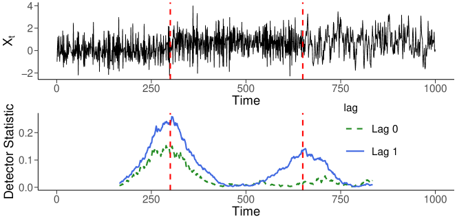
Figure 1: Top: time series of length $n=1000$ with change points $\theta_{1}=300$ and $\theta_{2}=650$ (vertical dashed lines), see Example 1. Bottom: corresponding detector statistics $T_{\ell}(G,k)$ computed at lags $\ell=0$ (dashed) and $\ell=1$ (solid).

Example 1.

A univariate time series $\{X_{t}\}_{t=1}^{n}$ of length $n=1000$ is generated as $X_{t}=\mu_{t}+\varepsilon_{t}$, where $\mu_{t}=0.7\cdot\mathbb{I}{\{t>\theta_{1}\}}$ and $\varepsilon_{t}=\varepsilon^{(1)}_{t}\cdot\mathbb{I}{\{t<\theta_{2}\}}+\varepsilon^{(2)}_{t}\cdot\mathbb{I}{\{t\geq\theta_{2}\}}$, with $\theta_{1}=300$ and $\theta_{2}=650$. Each $\varepsilon^{(j)}_{t}$ is an autoregressive (AR) process of order 1: $\varepsilon_{t}^{(1)}=0.5\varepsilon_{t-1}^{(1)}+W_{t}$ and $\varepsilon_{t}^{(2)}=-0.5\varepsilon_{t-1}^{(2)}+W_{t}$, where $\{W_{t}\}_{t\in\mathbb{Z}}$ is a white noise process with $\mathsf{Var}(W_{t})=\sqrt{1-0.5^{2}}$. This choice leads to $\mathsf{Var}(X_{t})=1$ for all $t$, see the top panel of Figure 1 for a realisation. Then, the mean shift at $\theta_{1}$ is detectable at all lags while the autocorrelation change at $\theta_{2}$ is detectable at odd lags only, i.e. $d^{(2)}_{\ell}=0$ for even $\ell\geq 0$. The bottom panel of Figure 1 plots $T_{\ell}(G,k),\,G\leq k\leq n-G$, computed using kernel $h_{2}$ in Lemma 2 (ii) with $G=166$. At lag $\ell=0$, the detector statistic forms a prominent peak around $\theta_{1}$ but it is flat around $\theta_{2}$; at lag $\ell=1$, the statistic $T_{1}(G,k)$ forms local maxima around both $\theta_{j},\,j=1,2$.

Based on these observations, it is reasonable to detect and locate the change points in the joint distribution of $(X_{t},X_{t+\ell})$ as significant local maximisers of $T_{\ell}(G,k)$. We adopt the selection criterion, first considered by Eichinger and Kirch, (2018) in the context of detecting mean shifts from univariate time series, for simultaneous estimation of multiple change points. For some fixed constant $\eta\in(0,1)$ and a threshold $\zeta_{\ell}(n,G)>0$, we identify any local maximiser of $T_{\ell}(G,k)$, say $\widehat{\theta}$, which satisfies

$$T_{\ell}(G,\widehat{\theta})>\zeta_{\ell}(n,G)\quad\text{and}\quad\widehat{\theta}={\operatorname*{arg\,max}}_{k:\,|k-\widehat{\theta}|\leq\eta G}T_{\ell}(G,k).$$ (4)

We denote the set of such estimators fulfilling (4) by $\widehat{\Theta}_{\ell}$ with $\widehat{q}_{\ell}=|\widehat{\Theta}_{\ell}|$. The choice of $\zeta_{\ell}(n,G)$ is discussed in Section 3.4.

3.2 Theoretical properties

For some finite integer $\ell\geq 0$, we define the index set of the change points detectable at lag $\ell$ as $\mathcal{I}_{\ell}=\{1\leq j\leq q:\,d^{(j)}_{\ell}\neq 0\}$, and denote its cardinality by $q_{\ell}=|\mathcal{I}_{\ell}|\leq q$. Not all change points are detectable at all lags, see Example 1 where we have $\mathcal{I}_{0}=\{1\}$ and $\mathcal{I}_{1}=\{1,2\}$. In this section, we show that the single-lag NP-MOJO described in Section 3.1 consistently estimates the total number $q_{\ell}$ and the locations $\{\theta_{j},\,j\in\mathcal{I}_{\ell}\}$ of the change points detectable at lag $\ell$, by $\widehat{\Theta}_{\ell}$.

Writing $g_{ti}(\cdot)=\sum_{j=0}^{q}g^{(j)}_{i}(\cdot)\cdot\mathbb{I}{\{\theta_{j}+1\leq t\leq\theta_{j+1}\}}$, define $X_{ti,\{t-s\}}=g_{ti}(\mathcal{F}_{t,\{t-s\}})$, where $F_{t,\{t-s\}}=\sigma(\ldots,\varepsilon_{t-s-1},\tilde{\varepsilon}_{t-s},\varepsilon_{t-s+1},\ldots,\varepsilon_{t})$ is a coupled version of $\mathcal{F}_{t}$ with $\varepsilon_{t-s}$ replaced by its independent copy $\tilde{\varepsilon}_{t-s}$. For a random variable $Z$ and $\nu>0$, let $\|Z\|_{\nu}=(\mathbb{E}(|Z|^{\nu}))^{1/\nu}$. Analogously as in Xu et al., 2022a , we define the element-wise functional dependence measure and its cumulative version as

$$\delta_{s,\nu,i}=\sup_{t\in\mathbb{Z}}\|X_{ti}-X_{ti,\{t-s\}}\|_{\nu}\text{ \ and \ }\Delta_{m,\nu}=\max_{1\leq i\leq p}\sum_{s=m}^{\infty}\delta_{s,\nu,i},\ m\in\mathbb{Z}.$$ (5)

Then, we make the following assumptions on the degree of serial dependence in $\{X_{t}\}_{t=1}^{n}$.

Assumption 1.

There exist some constants $C_{F},C_{X}\in(0,\infty)$ and $\gamma_{1}\in(0,2)$ such that

$$\sup_{m\geq 0}\exp(C_{F}m^{\gamma_{1}})\Delta_{m,2}\leq C_{X}.$$

Assumption 2.

The time series $\{X_{t}\}_{t=1}^{n}$ is continuous and $\beta$-mixing with $\beta(m)\leq C_{\beta}m^{-\gamma_{2}}$ for some constants $C_{\beta}\in(0,\infty)$ and $\gamma_{2}\geq 1$, where

$$\beta(m)=\sup_{t\in\mathbb{Z}}\left(\sup\frac{1}{2}\sum_{r=1}^{R}\sum_{s=1}^{S}\left|\mathsf{P}(A_{r}\cap B_{s})-\mathsf{P}(A_{r})\mathsf{P}(B_{s})\right|\right).$$

Here, the inner supremum is taken over all pairs of finite partitions $\{A_{1},\ldots,A_{R}\}$ of $\mathcal{F}_{t}=\sigma(\varepsilon_{u},\,u\leq t)$ and $\{B_{1},\ldots,B_{S}\}$ of $\sigma(\varepsilon_{u},\,u\geq t+m)$.

Assumptions 1 and 2 require the serial dependence in $\{X_{t}\}_{t=1}^{n}$, measured by $\Delta_{m,2}$ and $\beta(m)$, to decay exponentially, and both are met by a range of linear and non-linear processes (Wu,, 2005; Mokkadem,, 1988). Under Assumption 1, we have $\|X_{it}\|_{2}<\infty$ for all $i$ and $t$. Assumption 1 is required for bounding $T_{\ell}(G,k)-\mathbb{E}[T_{\ell}(G,k)]$ uniformly over $k$, while Assumption 2 is used for controlling the bias $\mathbb{E}[T_{\ell}(G,k)]-\mathcal{D}_{\ell}(G,k)$ which is attributed to serial dependence. A condition similar to Assumption 2 is often found in the time series literature making use of distance correlations, see e.g. Davis et al., (2018) and Yousuf and Feng, (2022).

Assumption 3.

The kernel function $h$ is symmetric and bounded, and can be written as $h(x,y)=h_{0}(x-y)$ for some function $h_{0}:\mathbb{R}^{2p}\to\mathbb{R}$ that is Lipschitz continuous with respect to $\|\cdot\|$ with Lipschitz constant $C_{h}\in(0,\infty)$.

Assumption 3 on the kernel function $h$ is met by $h_{1}$ and $h_{2}$ introduced in Lemma 2, with constants $C_{h}$ bounded by $\beta e^{-1/2}$ and $2\sqrt{2}p^{3/2}\delta^{-1/2}$, respectively.

Assumption 4.

1. $G=G_{n}$ satisfies $G^{-1}\log(n)\to 0$ as $n\to\infty$, and $\min_{0\leq j\leq q}(\theta_{j+1}-\theta_{j})\geq 2G$.

2. ${\sqrt{G/\log(n)}}\min_{j\in\mathcal{I}_{\ell}}d^{(j)}_{\ell}\to\infty$.

Recall that $\mathcal{I}_{\ell}$ denotes the index set of detectable change points at lag $\ell$, i.e. $d^{(j)}_{\ell}>0$ iff $j\in\mathcal{I}_{\ell}$. However, this definition of detectability is too weak to ensure that all $\theta_{j},\,j\in\mathcal{I}_{\ell}$, are detected by NP-MOJO with high probability at lag $\ell$, since we do not rule out the case of local changes where $d^{(j)}_{\ell}~{}\to~{}0$. Consider Example 1: the change in the autocorrelations results in $d^{(2)}_{\ell}>0$ for all odd $\ell$ but the size of change is expected to decay exponentially fast as $\ell$ increases. Assumption 4 allows for local changes provided that $\sqrt{G/\log(n)}d^{(j)}_{\ell}$ diverges sufficiently fast. Assumption 4 (i) on the minimum spacing of change points, is commonly imposed in the literature on change point detection using moving window-based procedures. Assumption 4 does not rule out $G/n\to 0$ and permits the number of change points $q$ to increase in $n$. We discuss the selection of bandwidth in Section 4.

Theorem 1.

Let Assumptions 1, 2, 3 and 4 hold and $\ell\geq 0$ be a finite integer, and set the threshold as $\zeta_{\ell}(n,G)=c_{\zeta}\sqrt{\log(n)/G}$ for some constant $c_{\zeta}>0$. Then, there exists $c_{0}>0$, depending only on $C_{F}$, $C_{X}$, $\gamma_{1}$, $C_{\beta}$ and $\gamma_{2}$, such that as $n\to\infty$,

$$\mathsf{P}\left(\widehat{q}_{\ell}=q_{\ell},\,\max_{j\in\mathcal{I}_{\ell}}\min_{\widehat{\theta}\in\widehat{\Theta}_{\ell}}\,d^{(j)}_{\ell}|\widehat{\theta}-\theta_{j}|\leq c_{0}\sqrt{G\log(n)}\right)\to 1.$$

Theorem 1 establishes that, for given $\ell$, NP-MOJO correctly estimates the total number and the locations of the change points detectable at lag $\ell$. In particular, by Assumption 4, the change point estimators satisfy

$$\min_{\widehat{\theta}\in\widehat{\Theta}_{\ell}}\,|\widehat{\theta}-\theta_{j}|=O_{P}((d^{(j)}_{\ell})^{-1}\sqrt{G\log(n)})=o_{P}(\min(\theta_{j}-\theta_{j-1},\theta_{j+1}-\theta_{j}))\text{ \ for all \ }j\in\mathcal{I}_{\ell},$$

i.e. the change point estimators converge to the true change point locations in the rescaled time. Further, the rate of estimation is inversely proportional to the size of change $d^{(j)}_{\ell}$, such that the change points associated with larger $d^{(j)}_{\ell}$ are estimated with better accuracy. Also making use of the energy-based distributional discrepancy, Matteson and James, (2014) establish the consistency of their proposed E-Divisive method for detecting changes in (marginal) distribution under independence. In addition to detection consistency, we further derive the rate of estimation for NP-MOJO which is applicable to detect changes in complex time series dependence besides those in marginal distribution, in broader situations permitting serial dependence.

3.3 Multi-lag extension of NP-MOJO

In this section, we address the problem of combining the results of the NP-MOJO procedure when it is applied with multiple lags. Let $\mathcal{L}\subset\mathbb{N}_{0}=\{0,1,\ldots\}$ denote a (finite) set of non-negative integers. Recall that given $\ell\in\mathcal{L}$, NP-MOJO returns a set of change points estimators $\widehat{\Theta}_{\ell}$. Denote the union of change point estimators over all lags $\mathcal{L}$ by $\widetilde{\Theta}=\bigcup_{\ell\in\mathcal{L}}\widehat{\Theta}_{\ell}=\{\widetilde{\theta}_{j},\,1\leq j\leq Q:\,\widetilde{\theta}_{1}<\ldots,<\widetilde{\theta}_{Q}\}$, and denote by $\mathbb{T}(\widetilde{\theta})=\max_{\ell\in\mathcal{L}}T_{\ell}(G,\widetilde{\theta})$ the maximum detector statistic at $\widetilde{\theta}$ across all $\ell\in\mathcal{L}$. We propose to find a set of the final change point estimators $\widehat{\Theta}\subset\widetilde{\Theta}$ by taking the following steps; we refer to this procedure as multi-lag NP-MOJO.

1. Set $\widehat{\Theta}=\emptyset$ and select a constant $c\in(0,2]$.

2. Set $\widetilde{\Theta}_{1}=\widetilde{\Theta}$ and $m=1$. Iterate Steps 2–4 for $m=1,2,\ldots$, while $\widetilde{\Theta}_{m}\neq\emptyset$.

3. Let $\widetilde{\theta}_{m}=\min\,\widetilde{\Theta}_{m}$ and identify $\mathcal{C}_{m}=\{\widetilde{\theta}\in\widetilde{\Theta}_{m}:\,\widetilde{\theta}-\widetilde{\theta}_{m}<cG\}$.

4. Identify $\widehat{\theta}_{m}=\operatorname*{arg\,max}_{\widetilde{\theta}\in\mathcal{C}_{m}}\mathbb{T}(\widetilde{\theta})$; if there is a tie, we arbitrarily break it.

5. Add $\widehat{\theta}_{m}$ to $\widehat{\Theta}$ and update $m\leftarrow m+1$ and $\widetilde{\Theta}_{m}=\widetilde{\Theta}_{m-1}\setminus\mathcal{C}_{m-1}$.

At iteration $m$ of the multi-lag NP-MOJO, Step 2 identifies the minimal element from the current set of candidate change point estimators $\widetilde{\Theta}_{m}$, and a cluster of estimators $\mathcal{C}_{m}$ whose elements are expected to detect the identical change points from multiple lags. Then, Step 3 finds an estimator $\widehat{\theta}\in\mathcal{C}_{m}$, which is associated with the largest detector statistic at some lag, and it is added to the set of final estimators. This choice is motivated by Theorem 1, which shows each $\theta_{j}$ is estimated with better accuracy at the lag associated with the largest change in the lagged dependence (measured by $d^{(j)}_{\ell}$). Iterating these steps until all the elements of $\widetilde{\Theta}$ are either added to $\widehat{\Theta}$ or discarded, we obtain the set of final change point estimators.

We define a subset of $\mathcal{L}$ containing the lags at which the $j$-th change point is detectable, as $\mathcal{L}^{(j)}=\{\ell\in\mathcal{L}:\,d^{(j)}_{\ell}\neq 0\}$. Re-visiting Example 1, when we set $\mathcal{L}=\{0,1\}$, it follows that $\mathcal{L}^{(1)}=\{0,1\}$ and $\mathcal{L}^{(2)}=\{1\}$. To establish the consistency of the multi-lag NP-MOJO, we formally assume that all changes points are detectable at some lag $\ell\in\mathcal{L}$.

Assumption 5.

For $\mathcal{L}\subset\mathbb{N}_{0}$ with $L=|\mathcal{L}|<\infty$, we have $\cup_{\ell\in\mathcal{L}}\mathcal{I}_{\ell}=\{1,\ldots,q\}$. Equivalently, $\mathcal{L}^{(j)}\neq\emptyset$ for all $j=1,\ldots,q$.

Under Assumptions 1–5, the consistency of the multi-lag NP-MOJO procedure is largely a consequence of Theorem 1. Assumption 4 (ii) requires that at any lag $\ell\in\mathcal{L}$ and a given change point $\theta_{j}$, we have either $j\in\mathcal{I}_{\ell}$ with $d^{(j)}_{\ell}$ large enough (in the sense that $\sqrt{G/\log(n)}d^{(j)}_{\ell}\to\infty$), or $j\notin\mathcal{I}_{\ell}$ such that $d^{(j)}_{\ell}=0$. Such a dyadic classification of the change points rules out the possibility that for some $j$, we have $d^{(j)}_{\ell}>0$ but $d^{(j)}_{\ell}=O(\sqrt{\log(n)/G})$, in which case $\theta_{j}$ may escape detection by NP-MOJO at lag $\ell$. We therefore consider the following alternative:

Assumption 6.

1. $G=G_{n}$ satisfies $G^{-1}\log(n)\to 0$ as $n\to\infty$, and $\min_{0\leq j\leq q}(\theta_{j+1}-\theta_{j})\geq 4G$.

2. $\sqrt{G/\log(n)}\min_{1\leq j\leq q}\max_{\ell\in\mathcal{L}^{(j)}}d^{(j)}_{\ell}\to\infty$.

Compared to Assumption 4, Assumption 6 requires that the change points are further apart from one another relative to $G$ by the multiplicative factor of two. At the same time, the latter only requires that for each $j=1,\ldots,q$, there exists at least one lag $\ell\in\mathcal{L}$ at which $d^{(j)}_{\ell}$ is large enough to guarantee the detection of $\theta_{j}$ by NP-MOJO with large probability. Theorem 2 establishes the consistency of multi-lag NP-MOJO under either Assumption 4 or 6.

Theorem 2.

Suppose that Assumptions 1, 2, 3 and 5 hold and at each $\ell\in\mathcal{L}$, we set $\zeta_{\ell}(n,G)=c_{\zeta,\ell}\sqrt{\log(n)/G}$ with some constants $c_{\zeta,\ell}>0$. Let $\widehat{\Theta}=\{\widehat{\theta}_{j},\,1\leq j\leq\widehat{q}:\,\widehat{\theta}_{1}<\ldots\widehat{\theta}_{\widehat{q}}\}$ denote the set of estimators returned by multi-lag NP-MOJO with tuning parameter $c$.

1. If Assumption 4 holds for all $\ell\in\mathcal{L}$ and $c=2\eta$ with $\eta\in(0,1/2]$, then with $c_{0}$ in Theorem 1,

   $$\mathsf{P}\left(\widehat{q}=q,\,\max_{1\leq j\leq q}\max_{\ell\in\mathcal{L}^{(j)}}d^{(j)}_{\ell}\left|\widehat{\theta}_{j}-\theta_{j}\right|\leq c_{0}\sqrt{G\log(n)}\right)\to 1\text{ \ as \ }n\to\infty.$$

2. If Assumption 6 holds and $c=2$, then the conclusion of (i) holds.

Under Assumption 6 (ii), which is weaker than Assumption 4 (ii), we may encounter a situation where $\sqrt{G/\log(n)}d^{(j)}_{\ell}=O(1)$ while $d^{(j)}_{\ell}>0$ at some lag $\ell\in\mathcal{L}$. Then, we cannot guarantee that such $\theta_{j}$ is detected by NP-MOJO at lag $\ell$ and, even so, we can only show that its estimator $\widetilde{\theta}\in\widetilde{\Theta}_{\ell}$ satisfies $|\widetilde{\theta}-\theta_{j}|=O(G)$. This requires setting the tuning parameter $c$ maximally for the clustering in Step 2 of multi-lag NP-MOJO, see Theorem 2 (ii). At the same time, there exists a lag well-suited for the localisation of each change point and Step 3 identifies an estimator detected at such lag, and the final estimator inherits the rate of estimation attained at the favourable lag.

3.4 Threshold selection via dependent wild bootstrap

Theorem 1 gives the choice of the threshold $\zeta_{\ell}(n,G)=c_{\zeta}\sqrt{\log(n)/G}$ which guarantees the consistency of NP-MOJO in multiple change point estimation. The choice of $c_{\zeta}$ influences the finite sample performance of NP-MOJO but it depends on many unknown quantities involved in specifying the degree of serial dependence in $\{X_{t}\}_{t=1}^{n}$ (see Assumptions 1 and 2), which makes the theoretical choice of little practical use. Resampling is popularly adopted for the calibration of change point detection methods including threshold selection. However, due to the presence of serial dependence, permutation-based approaches such as that adopted in Matteson and James, (2014) or sample splitting adopted in Padilla et al., (2021) are inappropriate.

We propose to adopt the dependent wild bootstrap procedure proposed in Leucht and Neumann, (2013), in order to approximate the quantiles of $\max_{G\leq k\leq n-G}T_{\ell}(G,k)$ in the absence of any change point, from which we select $\zeta_{\ell}(n,G)$.

Let $\{W_{t}^{[r]}\}_{t=1}^{n-G}$ denote a bootstrap sequence generated as a Gaussian AR($1$) process with $\mathsf{Var}(W_{t}^{[r]})=1$ and the AR coefficient $\exp(-1/b_{n})$, where the sequence $\{b_{n}\}$ is chosen such that $b_{n}=o(n)$ and $\lim_{n\to\infty}b_{n}=\infty$. We construct bootstrap replicates using $\{W_{t}^{[r]}\}_{t=1}^{n-G}$ as $T^{[r]}_{\ell}=\max_{G\leq k\leq n-G}T^{[r]}_{\ell}(G,k)$, where

$$\begin{split}T^{[r]}_{\ell}(G,k)&=\frac{1}{(G-\ell)^{2}}\left(\sum_{s,t=k-G+1}^{k-\ell}\bar{W}^{[r]}_{s,k}\bar{W}^{[r]}_{t,k}h(Y_{s},Y_{t})+\sum_{s,t=k+1}^{k+G-\ell}\bar{W}^{[r]}_{s-G,k}\bar{W}^{[r]}_{t-G,k}h(Y_{s},Y_{t})\right.\\ &\qquad\qquad\qquad\qquad\left.-2\sum_{s=k-G+1}^{k-\ell}\sum_{t=k+1}^{k+G-\ell}\bar{W}^{[r]}_{s,k}\bar{W}^{[r]}_{t-G,k}h(Y_{s},Y_{t})\right),\end{split}$$

with $\bar{W}^{[r]}_{t,k}=W^{[r]}_{t}-(G-\ell)^{-1}\sum_{u={k}-G+1}^{{k}-\ell}W^{[r]}_{u}$. Independently generating $\{W^{[r]}_{t}\}_{t=1}^{n-G}$ for $r=1,\ldots,R$ ($R$ denoting the number of bootstrap replications), we store $T^{[r]}_{\ell}$ and select the threshold as $\zeta_{\ell}(n,G)=q_{1-\alpha}(\{T^{[r]}_{\ell}\}_{r=1}^{R})$, the $(1-\alpha)$-quantile of $\{T^{[r]}_{\ell}\}_{r=1}^{R}$ for the chosen level $\alpha\in(0,1]$. Additionally, we can compute the importance score for each $\widehat{\theta}\in\widehat{\Theta}_{\ell}$ as

$$s(\widehat{\theta})=\frac{\left|\left\{1\leq r\leq R:\,T_{\ell}(G,\widehat{\theta})\geq T^{[r]}_{\ell,r}\right\}\right|}{R+1}.$$ (6)

Taking a value between $0$ and $1$, the larger $s(\widehat{\theta})$ is, the more likely that there exists a change point close to $\widehat{\theta}$ empirically. The bootstrap procedure generalises to the multi-lag NP-MOJO straightforwardly. In practice, we observe that setting $\widehat{\theta}_{j}=\operatorname*{arg\,max}_{\tilde{\theta}\in\mathcal{C}_{j}}s(\tilde{\theta})$ (with some misuse of the notation, $s(\cdot)$ is computed at the relevant lag for each $\widetilde{\theta}$) works well in Step 3 of multi-lag NP-MOJO. This is attributed to the fact that this score inherently takes into account the varying scale of the detector statistics at multiple lags and ‘standardises’ the importance of each estimator. In all numerical experiments, our implementation of multi-lag NP-MOJO is based on this choice of $\widehat{\theta}_{j}$. We provide the algorithmic descriptions of NP-MOJO and its multi-lag extension in Algorithms 1 and 2 in Appendix A.3.

4 Implementation of NP-MOJO

In this section, we discuss the computational aspects of NP-MOJO and provide recommendations for the choice of tuning parameters based on extensive numerical results.

Computational complexity. Owing to the MOSUM-based approach, the cost of sequentially computing $T_{\ell}(G,k)$ from $T_{\ell}(G,k-1)$ is $O(G)$, giving the overall cost of computing $T_{\ell}(G,k),\,G\leq k\leq n-G$, as $O(nG)$. Exact details of the sequential update are given in Appendix A.1. The bootstrap procedure described in Section 3.4 is performed once per lag for simultaneously detecting multiple change points, in contrast with E-Divisive (Matteson and James,, 2014) that requires the permutation-based testing to be performed for detecting each change point. With $R$ bootstrap replications, the total computational cost is $O(|\mathcal{L}|RnG)$ for multi-lag NP-MOJO using the set of lags $\mathcal{L}$ and bootstrapping, as opposed to $O(Rqn^{2})$ for E-Divisive.

Kernel function. Based on empirical performance, we recommend the use of the kernel function $h_{2}$ in Lemma 2 (ii) with $\delta$ set using the ‘median trick’, a common heuristic used in kernel-based methods (Li et al.,, 2019). Specifically, we set $\delta$ to be a half the the median of all $\|Y_{s}-Y_{t}\|^{2}$ involved in the calculation of $T_{\ell}(G,k)$. For $p$-variate i.i.d. Gaussian data with common variance $\sigma^{2}$, this corresponds to $\delta\approx\sigma p$ as the dimension $p$ increases (Ramdas et al.,, 2015).

Bandwidth. Due to the nonparametric nature of NP-MOJO, it is advised to use a larger bandwidth than that shown to work well for the MOSUM procedure for univariate mean change detection (Eichinger and Kirch,, 2018). In practice, the practitioner may have prior knowledge that aids the choice of $G$. In our simulation studies and data applications, we set $G=\lfloor n/6\rfloor$. It is often found that using multiple bandwidths and merging the results improves the adaptivity of moving window-based procedures, such as the ‘bottom-up’ merging proposed by Messer et al., (2014) or the localised pruning of (Cho and Kirch,, 2022). We leave investigation into the multiscale extension of NP-MOJO for future research.

Parameters for change point estimation. We set $\eta=0.4$ in (4) following the recommendation in Meier et al., (2021). For multi-lag NP-MOJO, we set $c=1$ for clustering the estimators from multiple lags, a choice that lies between those recommended in Theorem 2 (i) and (ii), since we do not know whether Assumptions 4 or 6 hold in practice. To further guard against spurious estimators, we only accept those $\widehat{\theta}$ that lie in intervals of length greater than $\lfloor 0.02G\rfloor$ where the corresponding $T_{\ell}(G,k)$ exceeds $\zeta_{\ell}(n,G)$.

Parameters for the bootstrap procedure. The choice of $b_{n}$ sets the level of dependence in the multiplier bootstrap sequences. Leucht and Neumann, (2013) show that a necessary condition is that $\lim_{n\to\infty}(b_{n}^{-1}+b{{}_{n}}n^{-1})=0$, giving a large freedom for choice of $b_{n}$. We recommend $b_{n}=1.5n^{1/3}$, which works well in practice. In all numerical experiments, we use $R=499$ bootstrap replications with $\alpha=0.1$.

Set of lags $\mathcal{L}$. The choice of $\mathcal{L}$ depends on the practitioner’s interest and domain knowledge, a problem commonly faced by general-purpose change point detection methods, such as the choice of the quantile level in Vanegas et al., (2022), the parameter of interest in Zhao et al., (2022) and the estimating equation in Kirch and Reckruehm, (2022). For example, for monthly data, using $\mathcal{L}=\{0,3,12\}$ allows for detecting changes in the quarterly and yearly seasonality. Even when the interest lies in detecting changes in the marginal distribution only, it helps to jointly consider multiple lags, since any marginal distributional change is likely to result in changes in the joint distribution of $(X_{t},X_{t+\ell})$. In simulations, we use $\mathcal{L}=\{0,1,2\}$ which works well not only for detecting changes in the mean and the second-order structure, but also for detecting changes in (non-linear) serial dependence and higher-order characteristics.

5 Simulation study

We conduct extensive simulation studies with varying change point scenarios ($18$ where $q\geq 1$, $7$ with $q=0$). We provide complete descriptions of the simulation studies in Appendix B where, for comparison, we consider not only nonparametric but also parametric data segmentation procedures well-suited to detect the types of changes in consideration, which include changes in the mean, second-order and higher-order moments and serial dependence. In this section, we briefly discuss a selection of the results and compare both single-lag and multi-lag NP-MOJO (denoted by NP-MOJO-$\ell$ and NP-MOJO-$\mathcal{L}$ respectively), with the nonparametric competitors: E-Divisive (Matteson and James,, 2014), NWBS (Padilla et al.,, 2021), KCPA (Celisse et al.,, 2018; Arlot et al.,, 2019) and cpt.np (Haynes et al.,, 2017). E-Divisive and KCPA are applicable to multivariate data segmentation whilst NWBS and cpt.np are not. The scenarios are (all with $n=1000$):

1. $X_{t}=\sum_{j=0}^{3}\Sigma_{j}^{1/2}\mathbb{I}{\{\theta_{j}+1\leq t\leq\theta_{j+1}\}}\cdot\varepsilon_{t}$, where $\varepsilon_{t}=(\varepsilon_{1t},\varepsilon_{2t})^{\top}$ with $\varepsilon_{it}\sim_{\text{i.i.d.}}t_{5}$, $(\theta_{1},\theta_{2},\theta_{3})=(250,500,750)$, $\Sigma_{0}=\Sigma_{2}=\begin{pmatrix}1&0\\ 0&1\end{pmatrix}$ and $\Sigma_{1}=\Sigma_{3}=\begin{pmatrix}1&0.9\\ 0.9&1\end{pmatrix}$.

2. $X_{t}=X^{(j)}_{t}=a_{j}X^{(j)}_{t-1}+\varepsilon_{t}$ for $\theta_{j}+1\leq t\leq\theta_{j+1}$, where $q=2$, $(\theta_{1},\theta_{2})=(333,667)$ and $(a_{0},a_{1},a_{2})=(-0.8,0.8,-0.8)$.

3. $X_{t}=X^{(j)}_{t}=\sigma^{(j)}_{t}\varepsilon_{t}$ with $(\sigma_{t}^{(j)})^{2}=\omega_{j}+\alpha_{j}(X^{(j)}_{t-1})^{2}+\beta_{j}(\sigma^{(j)}_{t-1})^{2}$ for $\theta_{j}+1\leq t\leq\theta_{j+1}$, where $q=1$, $\theta_{1}=500$, $(\omega_{0},\alpha_{0},\beta_{0})=(0.01,0.7,0.2)$ and $(\omega_{1},\alpha_{1},\beta_{1})=(0.01,0.2,0.7)$.

4. $X_{t}=0.4X_{t-1}+\varepsilon_{t}$ where $\varepsilon_{t}\sim_{\text{i.i.d.}}\mathcal{N}(0,0.5^{2})$ for $t\leq\theta_{1}$ and $t\geq\theta_{2}+1$, and $\varepsilon_{t}\sim_{\text{i.i.d.}}\text{Exponential}(0.5)-0.5$ for $\theta_{1}+1\leq t\leq\theta_{2}$, with $q=2$ and $(\theta_{1},\theta_{2})=(333,667)$.

The above scenarios consider: changes in the covariance of bivariate, non-Gaussian random vectors in (B5), changes in the autocorrelation (while the variance stays unchanged) in (C1), a change in the parameters of an ARCH($1$, $1$) process in (C3), and changes in higher moments of serially dependent observations in (D3). For further discussions of these scenarios, see Appendix B.2. Table LABEL:main-text-table reports the distribution of the estimated number of change points and the average covering metric (CM) and V-measure (VM) over 1000 realisations. Taking values between $[0,1]$, CM and VM close to $1$ indicates better accuracy in change point location estimation, see Appendix B.2 for their definitions. In the case of (C1), $q_{\ell}=0$ except for $q_{1}=2$, and thus we report $\widehat{q}_{\ell}-q_{\ell}$ for single-lag NP-MOJO. Across all scenarios, NP-MOJO-$\mathcal{L}$ shows good detection and estimation accuracy and demonstrates the efficacy of considering multiple lags, see (C3) and (D3) in particular. As the competitors are calibrated for the independent setting, they tend to either over- or under-detect the number of change points in the presence of serial dependence in (C1), (C3) and (D3). In Appendix B.2, we compare NP-MOJO against change point methods proposed for time series data where it similarly performs well.

Table 1: Distribution of the estimated number of change points and the average CM and VM over 1000 realisations. The modal value of $\widehat{q}-q$ in each row is given in bold. Also, the best performance for each metric is underlined for each scenario.

		$\widehat{q}-q$ / $\widehat{q}_{\ell}-q_{\ell}$
Model	Method	$\leq-2$	$-1$	$\mathbf{0}$	$1$	$\geq 2$	CM	VM
(B5)	NP-MOJO-$0$	0.000	0.001	0.997	0.002	0.000	0.974	0.959
	NP-MOJO-$1$	0.005	0.121	0.867	0.007	0.000	0.931	0.927
	NP-MOJO-$2$	0.006	0.103	0.884	0.007	0.000	0.935	0.929
	NP-MOJO-$\mathcal{L}$	0.000	0.001	0.999	0.000	0.000	0.973	0.958
	E-Divisive	0.670	0.189	0.101	0.032	0.008	0.431	0.335
	KCPA	0.322	0.000	0.662	0.015	0.001	0.775	0.725
(C1)	NP-MOJO-$0$	–	–	0.851	0.140	0.009	–	–
	NP-MOJO-$1$	0.000	0.002	0.956	0.042	0.000	0.978	0.961
	NP-MOJO-$2$	–	–	0.836	0.149	0.015	–	–
	NP-MOJO-$\mathcal{L}$	0.000	0.002	0.986	0.012	0.000	0.980	0.963
	E-Divisive	0.001	0.001	0.012	0.035	0.951	0.685	0.686
	KCPA	0.792	0.002	0.065	0.025	0.116	0.399	0.132
	NWBS	0.013	0.001	0.007	0.015	0.964	0.398	0.558
	cpt.np	0.000	0.000	0.002	0.003	0.995	0.593	0.647
(C3)	NP-MOJO-$0$	–	0.409	0.533	0.056	0.002	0.744	0.484
	NP-MOJO-$1$	–	0.236	0.682	0.081	0.001	0.819	0.633
	NP-MOJO-$2$	–	0.299	0.626	0.073	0.002	0.787	0.571
	NP-MOJO-$\mathcal{L}$	–	0.210	0.727	0.062	0.001	0.823	0.645
	E-Divisive	–	0.032	0.327	0.211	0.430	0.742	0.602
	KCPA	–	0.418	0.262	0.171	0.149	0.667	0.370
	NWBS	–	0.895	0.048	0.020	0.037	0.525	0.069
	cpt.np	–	0.000	0.013	0.047	0.940	0.634	0.554
(D3)	NP-MOJO-$0$	0.003	0.139	0.809	0.049	0.000	0.899	0.872
	NP-MOJO-$1$	0.006	0.155	0.792	0.047	0.000	0.892	0.864
	NP-MOJO-$2$	0.021	0.248	0.685	0.045	0.001	0.848	0.819
	NP-MOJO-$\mathcal{L}$	0.002	0.082	0.914	0.002	0.000	0.917	0.884
	E-Divisive	0.005	0.002	0.072	0.118	0.803	0.681	0.707
	KCPA	0.441	0.012	0.481	0.052	0.014	0.667	0.500
	NWBS	0.047	0.015	0.139	0.124	0.675	0.680	0.676
	cpt.np	0.000	0.000	0.045	0.055	0.900	0.726	0.756

6 Data applications

6.1 California seismology measurements data set

We analyse a data set from the High Resolution Seismic Network, operated by the Berkeley Seismological Laboratory. Ground motion sensor measurements were recorded in three mutually perpendicular directions at $13$ stations near Parkfield, California, USA for $740$ seconds from 2am on December 23rd 2004. The data has previously been analysed in Xie et al., (2019) and Chen et al., (2022). Chen et al., (2022) pre-process the data by removing a linear trend and down-sampling, and the processed data is available in the ocd R package (Chen et al.,, 2020). According to the Northern California Earthquake Catalog, an earthquake of magnitude 1:47 Md hit near Atascadero, California (50 km away from Parkfield) at 02:09:54.01.

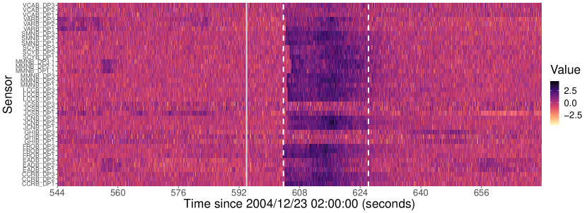
Figure 2: Heat map of standardised sensor data. Change points detected by multi-lag NP-MOJO are shown in vertical dashed lines, and the time of the earthquake is given by solid vertical line.

We analyse time series of dimension $p=39$ and length $n=2000$ by taking a portion of the data set between $544$ and $672$ seconds after $2$am, which covers the time at which the earthquake occurred ($594$ seconds after). We apply the multi-lag NP-MOJO with tuning parameters selected as in Section 4, using $G=333$ and set of lags $\mathcal{L}=\{0,\ldots,4\}$. We detect two changes at all lags; the first occurs at between 603.712 and 603.968 seconds after 2am and may be attributed to the earthquake. As noted in Chen et al., (2022), P waves, which are the primary preliminary wave and arrive first after an earthquake, travel at up to $6$km/s in the Earth’s crust. This is consistent with the delay of approximately $9$ seconds between the occurrence of the earthquake and the first change point detected by multi-lag NP-MOJO. We also note that performing online change point analysis, Xie et al., (2019) and Chen et al., (2022) report a change at 603.584 and 603.84 seconds after the earthquake, respectively. The second change is detected at between 626.176 and 626.496 seconds after 2am. It may correspond to the ending of the effect of the earthquake, as sensors return to ‘baseline’ behaviour. Figure 2 plots the heat map of the data with each series standardised for ease of visualisation, along with the onset of the earthquake and the two change points detected by the multi-lag NP-MOJO. It suggests, amongst other possible distributional changes, the time series undergoes mean shifts as found in Chen et al., (2022). We also examine the sample correlations computed on each of the three segments, see Figure 3 where the data exhibit a greater degree of correlation in segment $2$ compared to the other two segments. Recalling that each station is equipped with three sensors, we notice that pairwise correlations from the sensors located at the same stations undergo greater changes in correlations. A similar observation is made about the sensors located at nearby stations.

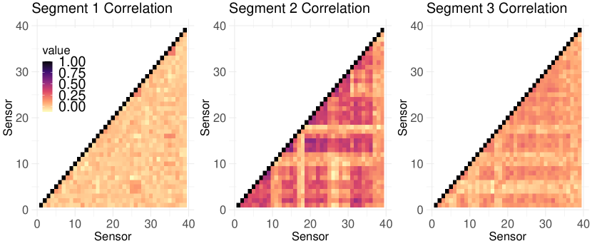
Figure 3: Sample correlations from the three segments defined by the change point estimators.

6.2 US recession data

We analyse the US recession indicator data set. Recorded quarterly between $1855$ and $2021$ ($n=667$), $X_{t}$ is recorded as a $1$ if any month in the quarter is in a recession (as identified by the Business Cycle Dating Committee of the National Bureau of Economic Research), and $0$ otherwise. The data has previously been examined for change points under piecewise stationary autoregressive models for integer-valued time series in Hudecová, (2013) and Diop and Kengne, (2021). We apply the multi-lag NP-MOJO with $G=111$ and $\mathcal{L}=\{0,\ldots,4\}$. All tuning parameters are set as recommended in Section 4 with one exception, $\delta$ for the kernel $h_{2}$. We select $\delta=1$ for lag $0$ and $2$ otherwise, since pairwise distances for binary data are either $0$ or $1$ when $\ell=0$ such that the median heuristic would not work as desired.

At all lags, we detect a single change point located between 1933:Q1 and 1938:Q2. Multi-lag NP-MOJO estimates the change point at 1933:Q1, which is comparable to the previous analyses: Hudecová, (2013) report a change at 1933:Q1 and Diop and Kengne, (2021) at 1932:Q4. The change coincides with the ending of the Great Depression and beginning of World War II. The left panel of Figure 4 plots the detected change along with the sample average of $X_{t}$ over the two segments (superimposed on $\{X_{t}\}_{t=1}^{n}$), showing that the frequency of recession is substantially lower after the change. The right panel plots the detector statistics $T_{\ell}(G,k)$ at lags $\ell\in\mathcal{L}$, divided by the respective threshold $\zeta_{\ell}(n,G)$ obtained from the bootstrap procedure. The thus-standardised $T_{4}(G,k)$, shown in solid line, displays the change point with the most clarity, attaining the largest value over the widest interval above the threshold (standardised to be one). At lag $4$, the detector statistic has the interpretation of measuring any discrepancy in the joint distribution of the recession indicator series and its yearly lagged values.

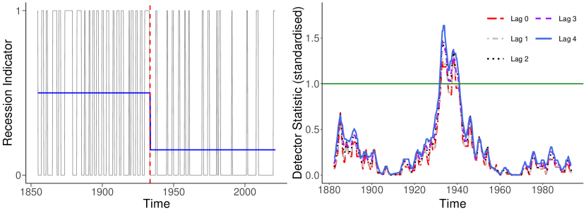
Figure 4: Left: quarterly US recession indicator series. A change point detected by multi-lag NP-MOJO is shown in vertical dashed lines and the sample means over the two segments in solid line. Right: $T_{\ell}(G,k),\,G\leq k\leq n-G$ for lags $\ell\in\mathcal{L}$, after standardisation by respective thresholds.

Appendix A Additional discussions about NP-MOJO

A.1 Computational complexity

As briefly discussed in Section 4, we can perform a sequential update of $T_{\ell}(G,k)$ to enable efficient computation. By symmetry of the kernel $h$, we only need to calculate $h(Y_{s},Y_{t})$ for $(s,t)$ satisfying $1\leq t\leq s\leq n$ and $|s-t|\leq 2G-\ell$, giving $O(nG)$ total computations for evaluating $h(Y_{s},Y_{t})$ for such $s$ and $t$. Then, writing

$$T_{\ell}(G,k) =\frac{1}{(G-\ell)^{2}}\left(\sum_{s,t=k-G+1}^{k-\ell}h(Y_{s},Y_{t})+\sum_{s,t=k+1}^{k+G-\ell}h(Y_{s},Y_{t})-2\sum_{s=k-G+1}^{k-\ell}\sum_{t=k+1}^{k+G-\ell}h(Y_{s},Y_{t})\right)$$

$$=:T^{(1)}_{\ell}(G,k)+T^{(1)}_{\ell}(G,k+G)-2T^{(2)}_{\ell}(G,k),$$

we can sequentially update $T^{(1)}_{\ell}(G,k)$ and $T^{(2)}_{\ell}(G,k)$. For example,

$$T^{(1)}_{\ell}(G,k+1)= \,T^{(1)}_{\ell}(G,k)-2\sum_{s=k-G+1}^{k-\ell}h(Y_{s},Y_{k-G+1})+2\sum_{s=k-G+2}^{k-\ell+1}h(Y_{s},Y_{k-G+2})$$

$$+h(Y_{k-G+1},Y_{k-G+1})-h(Y_{k-G+2},Y_{k-G+2}),$$

and a similar updating equation is available for $T^{(2)}_{\ell}(G,k)$. This update can be performed efficiently by pre-computing $\sum_{s=k-G+1}^{k-\ell}h(Y_{s},Y_{k-G+u})$ for all $k$ and $u=1,2$, which requires $O(n)$ computations. In a similar fashion, the bootstrap replicates $T^{[r]}_{\ell},\,1\leq\ell\leq R$, can also be computed using sequential updates in $O(nG)$ computational cost, giving the total cost for multi-lag NP-MOJO using the set of lags $\mathcal{L}$ as $O(|\mathcal{L}|RnG)$.

A.2 Alternative weight function

The following lemma describes the use of an additional weight function and kernel pair, supplementing Lemma 2 in the main text.

Lemma A.1.

For any $\gamma\in(0,2)$, suppose that $d^{(j)}_{\ell}$ is obtained with

$$w_{3}(u,v)=C_{3}(\gamma,p)^{-1}\left(\|u\|^{2}+\|v\|^{2}\right)^{-(\gamma+2p)/2}\text{ \ with \ }C_{3}(\gamma,p)=\frac{2\pi^{p/2}\Gamma(1-\gamma/2)}{\gamma 2^{\gamma}\Gamma((p+\gamma)/2)}.$$

If $\max_{0\leq j\leq q}\max_{1\leq i\leq p}\mathbb{E}(|X_{1i}^{(j)}|^{\gamma})\leq C<\infty$, then the function $h_{3}:\mathbb{R}^{2p}\times\mathbb{R}^{2p}\to[0,\infty)$ defined as $h_{3}(x,y)=\|x-y\|^{\gamma}$ for $x,y\in\mathbb{R}^{2p}$, satisfies

$$d^{(j)}_{\ell} =2\mathbb{E}\left[h_{3}\left(\tilde{Y}_{1}^{(j)},Y_{1}^{(j-1)}\right)\right]-\mathbb{E}\left[h_{3}\left(Y_{1}^{(j)},\tilde{Y}_{1}^{(j)}\right)\right]-\mathbb{E}\left[h_{3}\left(Y_{1}^{(j-1)},\tilde{Y}_{1}^{(j-1)}\right)\right].$$

The weight function $w_{3}$ was previously used in Bakirov et al., (2006) in the context of independence testing and in Matteson and James, (2014) for measuring changes in the marginal distribution of independent data (with $\ell=0$). In contrast to $w_{1}$ and $w_{2}$ given in Lemma 2, $w_{3}$ is non-separable and non-integrable, and does not fulfil Assumption 3. As a consequence, we require an additional condition on the moments of $X_{t}$ for $d^{(j)}_{\ell}$ to be well-defined as well as for the consistency of NP-MOJO when it is applied with the kernel $h_{3}$.

A.3 Algorithms

The algorithmic descriptions of the NP-MOJO procedure is summarised in Algorithms 1 and 2, corresponding to the single lag and multi-lag versions respectively.

Input: Multivariate time series $\{X_{t}\}_{t=1}^{n}$, bandwidth $G$, lag $\ell$, kernel $h$, selection parameter $\eta$, threshold level $\alpha$, bootstrap parameters $b_{n}$ and $R$

for $k\in\{G,\ldots,n-G\}$ do

       Compute $T_{\ell}(G,k)$

      

for $r\in\{1,...,R\}$ do

       Compute $T^{[r]}_{\ell}$

      

$\zeta_{\ell}(n,G)\leftarrow q_{1-\alpha}(\{T^{[r]}_{\ell}\}_{r=1}^{R})$

$\widehat{\Theta}_{\ell}\leftarrow$ Set of change point estimators obtained with bandwidth $G$ and threshold $\zeta_{\ell}(n,G)$ according to (4)

for $\widehat{\theta}\in\widehat{\Theta}_{\ell}$ do

       Compute $s(\widehat{\theta})$ according to Equation (6)

      

Output: Estimated change locations $\widehat{\Theta}_{\ell}$, change scores $\{s(\widehat{\theta}):\ \widehat{\theta}\in\widehat{\Theta}_{\ell}\}$

Algorithm 1 Single-lag NP-MOJO algorithm

Input: Multivariate time series $\{X_{t}\}_{t=1}^{n}$, bandwidth $G$, set of lags $\mathcal{L}$, kernel $h$, selection parameter $\eta$, threshold level $\alpha$, bootstrap parameters $b_{n}$ and $R$, merge parameter $c$

Initialise $\widehat{\Theta}\leftarrow\emptyset$

for $\ell\in\mathcal{L}$ do

       $\{\widehat{\Theta}_{\ell},\{s(\widehat{\theta}):\ \widehat{\theta}\in\widehat{\Theta}_{\ell}\}\}\leftarrow\textnormal{{NP-MOJO}}(\{X_{t}\}_{t=1}^{n},G,\ell,h,\eta,\alpha,b_{n},R)$

$\widetilde{\Theta}\leftarrow\bigcup_{\ell\in\mathcal{L}}\widehat{\Theta}_{\ell}$

$\widetilde{\Theta}_{1}\leftarrow\widetilde{\Theta}$, $j\leftarrow 1$

while $\widetilde{\Theta}_{j}\neq\emptyset$ do

       $\widehat{\theta}\leftarrow\min\widetilde{\Theta}_{j}$

       $\mathcal{C}_{j}\leftarrow\{\tilde{\theta}\in\widetilde{\Theta}_{j}:\tilde{\theta}-\widehat{\theta}<cG\}$

       $\widehat{\theta}_{j}\leftarrow\operatorname*{arg\,max}_{\tilde{\theta}\in\mathcal{C}_{j}}s(\tilde{\theta})$

       $\widehat{\Theta}\leftarrow\widehat{\Theta}\cup\{\widehat{\theta}_{j}\}$

       $\widetilde{\Theta}_{j+1}\leftarrow\widetilde{\Theta}_{j}\setminus\mathcal{C}_{j}$

       $j\leftarrow j+1$

Output: Estimated change locations $\widehat{\Theta}$, estimated number of changes $\widehat{q}=|\widehat{\Theta}|$

Algorithm 2 Multi-lag NP-MOJO algorithm

Appendix B Complete simulation study

We examine the performance of NP-MOJO via a wide-ranging simulation study. For all experiments we simulate $1000$ replications. All tuning parameters are set as described in Section 4. We report the results from both single-lag and multi-lag NP-MOJO with the set of lags $\mathcal{L}=\{0,1,2\}$, which are denoted by NP-MOJO-$\ell$ and NP-MOJO-$\mathcal{L}$, respectively.

Where appropriate, we compare with competing methods for which R implementations are readily available. In particular, we consider parametric methods which are designed specifically for detecting the particular types of changes we introduce in data generation, and their performance serve as a benchmark. Information about their implementation is given in the relevant sections.

For nonparametric methods, we consider the E-Divisive approach of Matteson and James, (2014) (R package ecp, James and Matteson, (2015)), the Kolmogorov-Smirnov-based CUSUM procedure (NWBS) of Padilla et al., (2021) implemented in the changepoints R package (Xu et al., 2022b, ), the kernel-based method (KCPA) of Celisse et al., (2018) and Arlot et al., (2019) (KernSeg, Rigaill and Marot, (2018)), and the computationally efficient extension of Zou et al., (2014) proposed by Haynes et al., (2017) (changepoint.np, Haynes and Killick, (2021)), referred to as cpt.np. In their implementation, we mostly follow the settings recommended by the authors. For E-Divisive and cpt.np, we set the minimum segment length to be $30$ and for the former, we use the same settings as NP-MOJO for the number of bootstrap replications $R$ and level $\alpha$. For cpt.np, we use the MBIC penalty for declaring change points and $10$ quantiles at which to estimate the cdf. For KCPA, we use the Gaussian kernel with bandwidth given by the standard deviation, and calculate the penalty using the slope heuristic as recommended in Arlot et al., (2019). We note that all four methods are developed for detecting changes in the marginal distribution from independent data. NWBS and cpt.np are univariate methods so their performance is not considered in the multivariate scenarios. Throughout, $\mathbf{0}$ denotes a vector of zeros and $\mathbf{I}$ an identity matrix, whose dimensions are determined by the context.

B.1 Size comparison

We assess the performance of NP-MOJO and nonparametric change point methods when there does not exist any change point in the time series. Unless stated otherwise, the time series is univariate ($p=1$) and $\varepsilon_{t}\sim_{\text{i.i.d.}}\mathcal{N}(0,\sigma_{\varepsilon}^{2})$ with $\sigma_{\varepsilon}=1$. In all scenarios, we set $n=1000$.

1. $X_{t}=\varepsilon_{t}$.

2. $X_{t}=\varepsilon_{t}$ where $\varepsilon_{t}$ are i.i.d. $t_{5}$-distributed random variables.

3. $X_{t}=0.7X_{t-1}+\varepsilon_{t}$.

4. $X_{t}=\varepsilon_{t}+0.9\varepsilon_{t-1}+0.8\varepsilon_{t-2}+0.7\varepsilon_{t-3}+0.6\varepsilon_{t-4}$.

5. $X_{t}=\sigma_{t}\varepsilon_{t}$ where $\sigma_{t}^{2}=0.5+0.4X_{t-1}^{2}$.

6. $X_{t}=AX_{t-1}+\varepsilon_{t}$ with $p=2$ where $\varepsilon_{t}\sim_{\text{i.i.d.}}\mathcal{N}_{2}(\mathbf{0},\mathbf{I})$ and $A=[A_{ii^{\prime}}]\in\mathbb{R}^{2\times 2}$ has $A_{11}=A_{22}=0.4,A_{12}=A_{21}=-0.2$.

7. $X_{t}=AX_{t-1}+\varepsilon_{t}$ with $p=5$ where $\varepsilon_{t}\sim_{\text{i.i.d.}}\mathcal{N}_{5}(\mathbf{0},\mathbf{I})$ and $A=[A_{ii^{\prime}}]\in\mathbb{R}^{5\times 5}$ has $A_{ii^{\prime}}=0.3^{|i-i^{\prime}|}$.

Table LABEL:null-table reports the proportion of realisations where change points are falsely detected. The single-lag NP-MOJO controls the size well across all scenarios. As expected, the multi-lag extension tends to return more spurious estimators but it shows reasonably good size performance. KCPA does not tend to return spurious estimators even when $\{X_{t}\}_{t=1}^{n}$ is serially correlated. On the other hand, E-Divisive, NWBS and cpt.np suffer from the presence of temporal dependence as they are calibrated for independent data. In the case of cpt.np, it tends to return spurious estimators even when the data is independently generated.

Table B.1: Size comparison: we report the size, the proportion of realisations where change points are falsely detected when $q=0$ out of $1000$ realisations.

Size	Model
Method	(N1)	(N2)	(N3)	(N4)	(N5)	(N6)	(N7)
NP-MOJO-$0$	0.043	0.050	0.123	0.104	0.064	0.045	0.021
NP-MOJO-$1$	0.061	0.058	0.116	0.100	0.043	0.053	0.016
NP-MOJO-$2$	0.059	0.065	0.138	0.116	0.082	0.064	0.026
NP-MOJO-$\mathcal{L}$	0.114	0.114	0.172	0.140	0.125	0.089	0.033
E-Divisive	0.109	0.112	1.000	1.000	0.167	0.631	0.999
KCPA	0.005	0.005	0.055	0.011	0.005	0.003	0.000
NWBS	0.049	0.037	0.841	0.791	0.103	–	–
cpt.np	0.286	0.313	1.000	1.000	0.695	–	–

B.2 Detection comparison

We investigate NP-MOJO in its change point detection performance in a variety of change point scenarios. Where relevant, we compare NP-MOJO with the relevant parametric change point detection methods, in addition to the nonparametric ones considered in Section B.1, and their performance serves as a benchmark.

For each scenario, we report the distribution of the error in estimating the number of change points. For single lag NP-MOJO, this refers to the distribution of $\widehat{q}_{\ell}-q_{\ell}$ (recall the definition of $q_{\ell}$ given in Section 3.2) over the $1000$ realisations, while for the multi-lag NP-MOJO and other methods, the distribution of $\widehat{q}-q$ is reported. We also report the covering metric (CM, Arbelaez et al.,, 2010) and V-measure (VM, Rosenberg and Hirschberg,, 2007) of the segmentation defined by the set of estimated change points. Let $\mathcal{P}=\{A_{j}\}_{j=1}^{q+1}$ denote the partition of $\{1,\ldots,n\}$ defined by the true change locations $\{\theta_{j}\}_{j=1}^{q}$, i.e. $A_{j}=\{\theta_{j-1}+1,\ldots,\theta_{j}\}$. Similarly we denote by $\widehat{\mathcal{P}}=\{\widehat{A}_{j}\}_{j=1}^{\widehat{q}+1}$ the partition defined by a set of estimated change points. Then, CM is defined as

$$\text{CM}(\widehat{\mathcal{P}},\mathcal{P})=\frac{1}{n}\sum_{A\in{\mathcal{P}}}|A|\max_{\widehat{A}\in{\widehat{\mathcal{P}}}}\left\{\frac{|A\cap\widehat{A}|}{|A\cup\widehat{A}|}\right\},$$

and advocated as an evaluation metric for comparing change point detection algorithms (van den Burg and Williams,, 2020). VM is similarly calculated using the conditional entropy of the resulting segmentation. Both the CM and VM take values between $0$ and $1$, with a value of $1$ indicating a perfect segmentation. For each measure, we report its average over the $1000$ realisations.

B.2.1 Changes in mean

We generate time series under the model

$$X_{t}=\sum_{j=0}^{q}\mu_{j}\mathbb{I}{\{\theta_{j}+1\leq t\leq\theta_{j}\}}+\varepsilon_{t},\,1\leq t\leq n,$$ (B.1)

with $n=1000$, $q=3$, $(\theta_{1},\theta_{2},\theta_{3})=(250,500,750)$ and $(\mu_{0},\mu_{1},\mu_{2},\mu_{3})=(0,{1},0,{1})$. The error sequence $\{\varepsilon_{t}\}_{t=1}^{n}$ is simulated according to models (N1)–(N4) from Section B.1, and then is standardised such that $\mathsf{Var}(\varepsilon_{t})=1$; we refer to the corresponding scenarios as (A1)–(A4). To these scenarios, in addition to the nonparametric methods considered in Section B.1, we apply the pruned exact linear time (PELT) method (Killick et al.,, 2012) implemented in the changepoint R package (Killick and Eckley,, 2014) and WCM.gSa (Cho and Fryzlewicz,, 2021) implemented in Anastasiou et al., (2022). While both detect multiple mean shifts in univariate time series, PELT is proposed for independent data while WCM.gSa handles autocorrelations under an AR model.

In addition, we consider a multivariate scenario:

1. Setting $p=10$, $X_{t}$ follows (B.1) with $\varepsilon_{t}\sim_{\text{i.i.d.}}\mathcal{N}_{10}(\mathbf{0},\mathbf{I})$ and $(\mu_{0},\mu_{1},\mu_{2},\mu_{3})=(\mathbf{0},\bm{\Delta},\mathbf{0},\bm{\Delta})$, where $\bm{\Delta}$ has its first $5$ coordinates set to $0.5$ and the rest to $0$.

The results are reported in Table LABEL:multcpt-a. In general, NP-MOJO accurately detects the number and locations of change points across all scenarios regardless of the choice of the lag, as the changes in the mean are detectable at all lags. In the independent settings (A1) and (A2), its performance is comparable to PELT while in the presence of serial dependence under (A3) and (A4), it performs as well as WCM.gSa. Among the nonparametric methods, NP-MOJO and KCPA outperform E-Divisive, NWBS and cpt.np and NP-MOJO tends to perform better than KCPA, either marginally or significantly, particularly in the multivariate setting in (A5). As noted in Section B.1, E-Dvisive, NWBS and cpt.np suffer from the departure from the independence assumption.

Table B.2: (A1)–(A5): we report the distribution of the estimated number of change points and the average CM and VM over 1000 realisations. The modal value of $\widehat{q}-q$ in each row is given in bold. Also, the best performance for each metric is underlined for each scenario.

		$\widehat{q}-q$
Model	Method	$\leq-2$	$-1$	$\mathbf{0}$	$1$	$\geq 2$	CM	VM
(A1)	NP-MOJO-$0$	0.000	0.019	0.976	0.005	0.000	0.958	0.942
	NP-MOJO-$1$	0.000	0.003	0.997	0.000	0.000	0.971	0.955
	NP-MOJO-$2$	0.000	0.002	0.997	0.001	0.000	0.971	0.955
	NP-MOJO-$\mathcal{L}$	0.000	0.001	0.999	0.000	0.000	0.970	0.953
	E-Divisive	0.000	0.000	0.912	0.070	0.018	0.975	0.965
	KCPA	0.000	0.000	0.971	0.028	0.001	0.977	0.963
	NWBS	0.000	0.000	0.955	0.028	0.017	0.971	0.956
	cpt.np	0.000	0.000	0.788	0.184	0.028	0.964	0.955
	PELT	0.000	0.000	1.000	0.000	0.000	0.983	0.970
	WCM.gSa	0.000	0.000	0.972	0.021	0.007	0.980	0.969
(A2)	NP-MOJO-$0$	0.000	0.002	0.998	0.000	0.000	0.974	0.958
	NP-MOJO-$1$	0.000	0.000	1.000	0.000	0.000	0.977	0.962
	NP-MOJO-$2$	0.000	0.000	0.999	0.001	0.000	0.976	0.961
	NP-MOJO-$\mathcal{L}$	0.000	0.000	1.000	0.000	0.000	0.976	0.961
	E-Divisive	0.000	0.000	0.913	0.058	0.029	0.977	0.969
	KCPA	0.000	0.000	0.978	0.021	0.001	0.983	0.972
	NWBS	0.000	0.000	0.970	0.015	0.015	0.979	0.967
	cpt.np	0.000	0.000	0.739	0.206	0.055	0.960	0.954
	PELT	0.000	0.000	1.000	0.000	0.000	0.983	0.970
	WCM.gSa	0.000	0.000	0.973	0.016	0.011	0.980	0.969
(A3)	NP-MOJO-$0$	0.000	0.000	0.999	0.001	0.000	0.986	0.978
	NP-MOJO-$1$	0.000	0.000	0.997	0.003	0.000	0.984	0.974
	NP-MOJO-$2$	0.000	0.000	0.997	0.003	0.000	0.984	0.973
	NP-MOJO-$\mathcal{L}$	0.000	0.000	1.000	0.000	0.000	0.984	0.975
	E-Divisive	0.000	0.000	0.001	0.000	0.999	0.413	0.675
	KCPA	0.000	0.000	0.724	0.151	0.125	0.959	0.962
	NWBS	0.000	0.000	0.000	0.000	1.000	0.438	0.662
	cpt.np	0.000	0.000	0.002	0.009	0.989	0.655	0.779
	PELT	0.000	0.000	0.233	0.244	0.523	0.885	0.914
	WCM.gSa	0.000	0.000	0.949	0.027	0.024	0.985	0.981
(A4)	NP-MOJO-$0$	0.000	0.000	0.996	0.004	0.000	0.980	0.969
	NP-MOJO-$1$	0.000	0.000	0.997	0.003	0.000	0.978	0.966
	NP-MOJO-$2$	0.000	0.000	0.997	0.003	0.000	0.977	0.964
	NP-MOJO-$\mathcal{L}$	0.000	0.000	1.000	0.000	0.000	0.979	0.967
	E-Divisive	0.000	0.000	0.000	0.000	1.000	0.416	0.674
	KCPA	0.000	0.000	0.910	0.062	0.028	0.978	0.972
	NWBS	0.000	0.000	0.001	0.000	0.999	0.437	0.658
	cpt.np	0.000	0.000	0.000	0.006	0.994	0.642	0.769
	PELT	0.000	0.000	0.309	0.272	0.419	0.905	0.923
	WCM.gSa	0.000	0.000	0.987	0.010	0.003	0.985	0.977
(A5)	NP-MOJO-$0$	0.001	0.013	0.986	0.006	0.000	0.971	0.957
	NP-MOJO-$1$	0.000	0.005	0.995	0.000	0.000	0.976	0.962
	NP-MOJO-$2$	0.000	0.004	0.996	0.000	0.000	0.976	0.961
	NP-MOJO-$\mathcal{L}$	0.000	0.003	0.997	0.000	0.000	0.975	0.961
	E-Divisive	0.000	0.000	0.913	0.072	0.015	0.978	0.969
	KCPA	1.000	0.000	0.000	0.000	0.000	0.250	0.000

B.2.2 Changes in second-order moments

We first consider the scenarios where $X_{t}$ undergoes changes in variance or covariance which are detectable at all lags, with $n=1000$, $q=3$ and $(\theta_{1},\theta_{2},\theta_{3})=(250,500,750)$.

1. $X_{t}=\sum_{j=0}^{q}\sigma_{j}\mathbb{I}{\{\theta_{j}+1\leq t\leq\theta_{j+1}\}}\cdot\varepsilon_{t}$ where $\varepsilon_{t}\sim_{\text{i.i.d.}}\mathcal{N}(0,1)$ and $(\sigma_{0},\sigma_{1},\sigma_{2},\sigma_{3})=(0.5,1,0.5,1)$.

2. $X_{t}=\sum_{j=0}^{q}\sigma_{j}\mathbb{I}{\{\theta_{j}+1\leq t\leq\theta_{j+1}\}}\cdot\varepsilon_{t}$ with $\sigma_{j}$ chosen as in (B1) where $\varepsilon_{t}\sim_{\text{i.i.d.}}t_{5}$.

3. $X_{t}=0.4X_{t-1}+\sum_{j=0}^{q}\sigma_{j}\mathbb{I}{\{\theta_{j}+1\leq t\leq\theta_{j+1}\}}\cdot\varepsilon_{t}$ where $\varepsilon_{t}\sim_{\text{i.i.d.}}\mathcal{N}(0,1)$ and $(\sigma_{0},\sigma_{1},\sigma_{2},\sigma_{3})=(1,0.2,1,0.2)$.

4. $X_{t}=\sum_{j=0}^{q}\Sigma_{j}^{1/2}\mathbb{I}{\{\theta_{j}+1\leq t\leq\theta_{j+1}\}}\cdot\varepsilon_{t}$ with $p=2$, where $\varepsilon_{t}\sim_{\text{i.i.d.}}\mathcal{N}_{2}(\mathbf{0},\mathbf{I})$, $\Sigma_{0}=\Sigma_{2}=\mathbf{I}$ and $\Sigma_{1}=\Sigma_{3}=\begin{pmatrix}1&0.9\\ 0.9&1\end{pmatrix}$.

5. As in (B4) where $\varepsilon_{t}=(\varepsilon_{1t},\varepsilon_{2t})^{\top}$ generated with $\varepsilon_{it}\sim_{\text{i.i.d.}}t_{5}$.

In addition to the nonparametric competitors, we consider the wavelet-based WBS approach (WBSTS) of Korkas and Fryzlewicz, (2017), implemented in the R package wbsts (Korkas and Fryzlewicz,, 2020), when $p=1$, and the sparsified binary segmentation (SBS) (Cho and Fryzlewicz,, 2015), implemetend in the R package hdbinseg (Cho and Fryzlewicz,, 2018) when $p>1$, both of which are developed for detecting changes in the second-order structure of time series. The results are reported in Table LABEL:multcpt-b. NP-MOJO consistently outperforms the competing nonparametric methods in all metrics. It is competitive with WBSTS and SBS which specifically seek changes in the second-order structure and in fact, NP-MOJO performs better in estimating $q$ when the data is non-Gaussian in model (B2).

Table B.3: (B1)–(B5): we report the distribution of the estimated number of change points and the average CM and VM over 1000 realisations. The modal value of $\widehat{q}-q$ in each row is given in bold. Also, the best performance for each metric is underlined for each scenario.

		$\widehat{q}-q$
Model	Method	$\leq-2$	$-1$	$\mathbf{0}$	$1$	$\geq 2$	CM	VM
(B1)	NP-MOJO-$0$	0.000	0.052	0.930	0.017	0.001	0.942	0.928
	NP-MOJO-$1$	0.000	0.008	0.986	0.006	0.000	0.965	0.949
	NP-MOJO-$2$	0.000	0.008	0.988	0.004	0.000	0.966	0.949
	NP-MOJO-$\mathcal{L}$	0.000	0.006	0.994	0.000	0.000	0.965	0.948
	E-Divisive	0.003	0.008	0.896	0.069	0.024	0.946	0.934
	KCPA	0.007	0.000	0.955	0.033	0.005	0.965	0.949
	NWBS	0.429	0.093	0.364	0.089	0.025	0.616	0.558
	cpt.np	0.000	0.000	0.676	0.214	0.110	0.943	0.936
	WBSTS	0.000	0.000	0.978	0.021	0.001	0.960	0.941
(B2)	NP-MOJO-$0$	0.005	0.133	0.839	0.023	0.000	0.912	0.905
	NP-MOJO-$1$	0.000	0.044	0.945	0.011	0.000	0.944	0.929
	NP-MOJO-$2$	0.000	0.033	0.956	0.011	0.000	0.945	0.929
	NP-MOJO-$\mathcal{L}$	0.000	0.012	0.988	0.000	0.000	0.950	0.932
	E-Divisive	0.035	0.039	0.814	0.096	0.016	0.910	0.902
	KCPA	0.100	0.003	0.863	0.032	0.002	0.904	0.882
	NWBS	0.559	0.136	0.212	0.064	0.029	0.510	0.423
	cpt.np	0.001	0.000	0.615	0.269	0.115	0.924	0.915
	WBSTS	0.000	0.002	0.693	0.230	0.075	0.905	0.894
(B3)	NP-MOJO-$0$	0.025	0.121	0.840	0.014	0.000	0.905	0.899
	NP-MOJO-$1$	0.000	0.024	0.962	0.014	0.000	0.953	0.937
	NP-MOJO-$2$	0.000	0.035	0.953	0.012	0.000	0.949	0.934
	NP-MOJO-$\mathcal{L}$	0.000	0.013	0.987	0.000	0.000	0.953	0.936
	E-Divisive	0.000	0.000	0.148	0.178	0.674	0.774	0.813
	KCPA	0.163	0.004	0.739	0.071	0.023	0.858	0.833
	NWBS	0.085	0.036	0.110	0.118	0.651	0.657	0.700
	cpt.np	0.000	0.000	0.046	0.105	0.849	0.789	0.831
	WBSTS	0.000	0.000	0.979	0.021	0.000	0.954	0.934
(B4)	NP-MOJO-$0$	0.000	0.000	1.000	0.000	0.000	0.981	0.967
	NP-MOJO-$1$	0.000	0.031	0.963	0.006	0.000	0.965	0.953
	NP-MOJO-$2$	0.000	0.015	0.976	0.009	0.000	0.969	0.955
	NP-MOJO-$\mathcal{L}$	0.000	0.000	1.000	0.000	0.000	0.979	0.965
	E-Divisive	0.529	0.168	0.256	0.032	0.015	0.557	0.506
	KCPA	0.077	0.000	0.909	0.014	0.000	0.935	0.915
	SBS	0.044	0.000	0.942	0.014	0.000	0.949	0.939
(B5)	NP-MOJO-$0$	0.000	0.001	0.997	0.002	0.000	0.974	0.959
	NP-MOJO-$1$	0.005	0.121	0.867	0.007	0.000	0.931	0.927
	NP-MOJO-$2$	0.006	0.103	0.884	0.007	0.000	0.935	0.929
	NP-MOJO-$\mathcal{L}$	0.000	0.001	0.999	0.000	0.000	0.973	0.958
	E-Divisive	0.670	0.189	0.101	0.032	0.008	0.431	0.335
	KCPA	0.322	0.000	0.662	0.015	0.001	0.775	0.725
	SBS	0.614	0.003	0.377	0.006	0.000	0.653	0.660

B.2.3 Changes in temporal dependence

We consider the scenarios where the autocorrelations or the (conditional) variance of the data change. Unless stated otherwise $q=2$, $(\theta_{1},\theta_{2})=(333,667)$ and $\varepsilon_{t}\sim_{\text{i.i.d.}}\mathcal{N}(0,1)$.

1. $X_{t}=X^{(j)}_{t}=a_{j}X^{(j)}_{t-1}+\varepsilon_{t}$ for $\theta_{j}+1\leq t\leq\theta_{j+1}$, where $(a_{0},a_{1},a_{2})=(-0.8,0.8,-0.8)$.

2. $X_{t}=\varepsilon_{t}+\sum_{j=0}^{q}b_{j}\mathbb{I}{\{\theta_{j}+1\leq t\leq\theta_{j+1}\}}\cdot\varepsilon_{t-2}$, where $(b_{0},b_{1},b_{2})=(-0.7,0.7,-0.7)$.

3. $X_{t}=X^{(j)}_{t}=\sigma^{(j)}_{t}\varepsilon_{t}$ with $(\sigma^{(j)}_{t})^{2}=\omega_{j}+\alpha_{j}(X^{(j)}_{t-1})^{2}+\beta_{j}(\sigma^{(j)}_{t-1})^{2})$ for $\theta_{j}+1\leq t\leq\theta_{j+1}$, $q=1$, $\theta_{1}=500$, $(\omega_{0},\alpha_{0},\beta_{0})=(0.01,0.7,0.2)$ and $(\omega_{1},\alpha_{1},\beta_{1})=(0.01,0.2,0.7)$.

4. $X_{t}=X^{(j)}_{t}=A_{j}X^{(j)}_{t-1}+\varepsilon_{t}$ for $\theta_{j}+1\leq t\leq\theta_{j+1}$, where $A_{0}=A_{2}=\begin{pmatrix}0.5&0.1\\ 0.1&0.5\end{pmatrix}$ and $A_{1}=\begin{pmatrix}-0.5&0.1\\ 0.1&-0.5\end{pmatrix}$.

5. $X_{t}=\varepsilon_{t}+\sum_{j=0}^{q}B_{j}\mathbb{I}{\{\theta_{j}+1\leq t\leq\theta_{j+1}\}}\cdot\varepsilon_{t-1}$, where $B_{0}=B_{2}=\begin{pmatrix}1&0.1\\ 0.1&1\end{pmatrix}$ and $B_{1}=\begin{pmatrix}-1&0.1\\ 0.1&-1\end{pmatrix}$.

Model 1 was studied in Korkas and Fryzlewicz, (2017), while models similar to 4 and 5 were considered in Preuß et al., (2015). In all models, except 3, changes are present only in the joint distribution of $X_{t}$ and its lagged values. Therefore, we exclude the nonparametric methods considered in Section B.1 which have detection power against changes in marginal distribution only. Specifically, $(q_{0},q_{1},q_{2})=(0,0,2)$ in 2 and $(q_{0},q_{1},q_{2})=(0,2,0)$ in 4 and 5. Accordingly, in reporting the results returned by NP-MOJO-$\ell$ for $\ell=0,1,2$, we report the distribution of $\widehat{q}_{\ell}-q_{\ell}$ and report CM and VM for NP-MOJO-$\ell$ with $q_{\ell}=2$ only, see Table LABEL:multcpt-c. We observe that NP-MOJO performs similarly or superior to the competing method in both detection and estimation accuracy. As expected, we do not detect all $q$ change points from NP-MOJO-$\ell$ for which $q_{\ell}<q$, but the multi-lag extension successfully aggregates the estimators from multiple lags.

Table B.4: 1–5: we report the distribution of the estimated number of change points and the average CM and VM over 1000 realisations. The modal value of $\widehat{q}-q$ in each row is given in bold. Also, the best performance for each metric is underlined for each scenario.

		$\widehat{q}-q$ / $\widehat{q}_{\ell}-q_{\ell}$
Model	Method	$-2$	$-1$	$\mathbf{0}$	$1$	$\geq 2$	CM	VM
1	NP-MOJO-$0$	–	–	0.851	0.140	0.009	–	–
	NP-MOJO-$1$	0.000	0.002	0.956	0.042	0.000	0.978	0.961
	NP-MOJO-$2$	–	–	0.836	0.149	0.015	–	–
	NP-MOJO-$\mathcal{L}$	0.000	0.002	0.986	0.012	0.000	0.980	0.963
	WBSTS	0.000	0.000	0.414	0.299	0.287	0.904	0.900
2	NP-MOJO-$0$	–	–	0.952	0.047	0.001	–	–
	NP-MOJO-$1$	–	–	0.930	0.068	0.002	–	–
	NP-MOJO-$2$	0.001	0.054	0.908	0.036	0.001	0.949	0.926
	NP-MOJO-$\mathcal{L}$	0.001	0.051	0.942	0.006	0.000	0.950	0.926
	WBSTS	0.007	0.021	0.899	0.062	0.011	0.896	0.852
3	NP-MOJO-$0$	–	0.409	0.533	0.056	0.002	0.744	0.484
	NP-MOJO-$1$	–	0.236	0.682	0.081	0.001	0.819	0.633
	NP-MOJO-$2$	–	0.299	0.626	0.073	0.002	0.787	0.571
	NP-MOJO-$\mathcal{L}$	–	0.210	0.727	0.062	0.001	0.823	0.645
	WBSTS	–	0.003	0.025	0.054	0.918	0.662	0.487
4	NP-MOJO-$0$	–	–	0.904	0.090	0.006	–	–
	NP-MOJO-$1$	0.004	0.159	0.783	0.051	0.003	0.907	0.893
	NP-MOJO-$2$	–	–	0.888	0.107	0.005	–	–
	NP-MOJO-$\mathcal{L}$	0.004	0.165	0.818	0.013	0.000	0.907	0.891
	SBS	0.070	0.000	0.911	0.019	0.000	0.903	0.875
5	NP-MOJO-$0$	–	–	0.939	0.058	0.003	–	–
	NP-MOJO-$1$	0.000	0.011	0.952	0.035	0.002	0.974	0.957
	NP-MOJO-$2$	–	–	0.926	0.073	0.001	–	–
	NP-MOJO-$\mathcal{L}$	0.000	0.012	0.979	0.009	0.000	0.976	0.957
	SBS	0.006	0.000	0.961	0.033	0.000	0.967	0.942

B.2.4 Changes in higher-order moments

We simulate scenarios where there are changes in stochastic properties beyond the first two moments. In what follows, we have $q=2$ and $(\theta_{1},\theta_{2})=(333,667)$.

1. $X_{t}\sim_{\text{i.i.d.}}\mathcal{N}(0,1)$ for $t\leq\theta_{1}$ and $t\geq\theta_{2}+1$, and $X_{t}\sim_{\text{ i.i.d.}}t_{2.5}/\sqrt{5}$ for $\theta_{1}+1\leq t\leq\theta_{2}$.

2. $X_{t}\sim_{\text{ i.i.d.}}0.5+(\chi^{2}_{1}-1)/2\sqrt{2}$ for $t\leq\theta_{1}$ and $t\geq\theta_{2}+1$, and $X_{t}\sim_{\text{ i.i.d.}}\mathcal{N}(0.5,0.5^{2})$ for $\theta_{1}+1\leq t\leq\theta_{2}$.

3. $X_{t}=0.4X_{t-1}+\varepsilon_{t}$ where $\varepsilon_{t}\sim_{\text{i.i.d.}}\mathcal{N}(0,0.5^{2})$ for $t\leq\theta_{1}$ and $t\geq\theta_{2}+1$, and $\varepsilon_{t}\sim_{\text{i.i.d.}}\text{Exponential}(0.5)-0.5$ for $\theta_{1}+1\leq t\leq\theta_{2}$.

Model 1 is taken from Padilla et al., (2021), where $\mathbb{E}(X_{t})=0$ and $\mathsf{Var}(X_{t})=1$ for all $t$ and changes occur in the tail of the distribution. Model 2 is a variation of a scenario studied in Arlot et al., (2019), where $\mathbb{E}(X_{t})=0.5$ and $\mathsf{Var}(X_{t})=0.25$ for all $t$ with changes in the tail behaviour. Model 3 considers changes in higher order moments but allows the data to be serially correlated. The results are reported in Table LABEL:multcpt-high, from which we see that the multi-lag NP-MOJO procedure gives the strongest overall performance, particularly in the serially correlated model 3. KCPA performs the best from the competing methods, and NWBS tends to under-detect the change points while cpt.np over-detects them.

Table B.5: 1–3: we report the distribution of the estimated number of change points and the average CM and VM over 1000 realisations. The modal value of $\widehat{q}-q$ in each row is given in bold. Also, the best performance for each metric is underlined for each scenario.

		$\widehat{q}-q$
Model	Method	$-2$	$-1$	$\mathbf{0}$	$1$	$\geq 2$	CM	VM
1	NP-MOJO-$0$	0.000	0.069	0.892	0.037	0.002	0.933	0.904
	NP-MOJO-$1$	0.003	0.134	0.810	0.053	0.000	0.902	0.874
	NP-MOJO-$2$	0.000	0.128	0.823	0.049	0.000	0.905	0.878
	NP-MOJO-$\mathcal{L}$	0.000	0.034	0.960	0.006	0.000	0.942	0.909
	E-Divisive	0.113	0.086	0.699	0.079	0.023	0.832	0.770
	KCPA	0.086	0.002	0.890	0.019	0.003	0.909	0.853
	NWBS	0.496	0.070	0.339	0.076	0.019	0.582	0.394
	cpt.np	0.006	0.004	0.592	0.276	0.122	0.896	0.864
2	NP-MOJO-$0$	0.000	0.005	0.981	0.014	0.000	0.970	0.944
	NP-MOJO-$1$	0.000	0.126	0.824	0.049	0.001	0.904	0.874
	NP-MOJO-$2$	0.001	0.105	0.831	0.060	0.003	0.909	0.879
	NP-MOJO-$\mathcal{L}$	0.000	0.003	0.993	0.004	0.000	0.964	0.934
	E-Divisive	0.000	0.000	0.894	0.058	0.048	0.956	0.931
	KCPA	0.104	0.001	0.880	0.014	0.001	0.897	0.835
	NWBS	0.350	0.000	0.508	0.101	0.041	0.731	0.596
	cpt.np	0.000	0.000	0.741	0.184	0.075	0.962	0.950
3	NP-MOJO-$0$	0.003	0.139	0.809	0.049	0.000	0.899	0.872
	NP-MOJO-$1$	0.006	0.155	0.792	0.047	0.000	0.892	0.864
	NP-MOJO-$2$	0.021	0.248	0.685	0.045	0.001	0.848	0.819
	NP-MOJO-$\mathcal{L}$	0.002	0.082	0.914	0.002	0.000	0.917	0.884
	E-Divisive	0.005	0.002	0.072	0.118	0.803	0.681	0.707
	KCPA	0.441	0.012	0.481	0.052	0.014	0.667	0.500
	NWBS	0.047	0.015	0.139	0.124	0.675	0.680	0.676
	cpt.np	0.000	0.000	0.045	0.055	0.900	0.726	0.756

Appendix C Proofs of main results

C.1 Proof of Lemma 1

If $g^{(j)}(\cdot)=g^{(j-1)}(\cdot)$, then $\phi^{(j)}_{\ell}(u,v)=\phi^{(j-1)}_{\ell}(u,v)$ for all $(u,v)$, which implies that $|\phi^{(j)}_{\ell}(u,v)-\phi^{(j-1)}_{\ell}(u,v)|^{2}\equiv 0$, and hence $d^{(j)}_{\ell}=0$ in (2). Conversely, suppose that $d_{\ell}^{(j)}=0$ for all $\ell\geq 0$. Then, $\phi^{(j)}_{\ell}(u,v)-\phi^{(j-1)}_{\ell}(u,v)=0$ a.e. since $w(u,v)>0$ for $u,v\neq 0$, and hence $g^{(j)}(\cdot)=g^{(j-1)}(\cdot)$.

C.2 Proof of Lemma 2

We first consider the integrand term in (2) involving the characteristic functions. We have that

$$\left|\phi^{(j)}_{\ell}(u,v)-\phi^{(j-1)}_{\ell}(u,v)\right|^{2} =\phi^{(j)}_{\ell}(u,v)\overline{\phi^{(j)}_{\ell}(u,v)}+\phi^{(j-1)}_{\ell}(u,v)\overline{\phi^{(j-1)}_{\ell}(u,v)}$$

$$\quad-\phi^{(j)}_{\ell}(u,v)\overline{\phi^{(j-1)}_{\ell}(u,v)}-\overline{\phi^{(j)}_{\ell}(u,v)}\phi^{(j-1)}_{\ell}(u,v)$$

$$=:A+B-C-D.$$

Then,

$$A =\mathbb{E}\left[\exp\left(\imath\langle u,X_{1}^{(j)}\rangle+\imath\langle v,X^{(j)}_{1+\ell}\rangle\right)\right]\mathbb{E}\left[\exp(-\imath\langle u,\widetilde{X}^{(j)}_{1}\rangle-\imath\langle v,\widetilde{X}^{(j)}_{1+\ell}\rangle)\right]$$

$$=\mathbb{E}\left[\exp\left(\imath\langle u,X^{(j)}_{1}-\widetilde{X}^{(j)}_{1}\rangle+\imath\langle v,X^{(j)}_{1+\ell}-\widetilde{X}^{(j)}_{1+\ell}\rangle\right)\right].$$

In a similar fashion,

$$B=\mathbb{E}\left[\exp\left(\imath\langle u,X_{1}^{(j-1)}-\widetilde{X}^{(j-1)}_{1}\rangle+\imath\langle v,X_{1+\ell}^{(j-1)}-\widetilde{X}^{(j-1)}_{1+\ell}\rangle\right)\right],$$

$$C=\mathbb{E}\left[\exp\left(\imath\langle u,\widetilde{X}^{(j)}_{1}-X^{(j-1)}_{1}\rangle+\imath\langle v,\widetilde{X}^{(j)}_{1+\ell}-X^{(j-1)}_{1+\ell}\rangle\right)\right],$$

$$D=\mathbb{E}\left[\exp\left(-\imath\langle u,\widetilde{X}^{(j)}_{1}-X^{(j-1)}_{1}\rangle-\imath\langle v,\widetilde{X}^{(j)}_{1+\ell}-X^{(j-1)}_{1+\ell}\rangle\right)\right].$$

Note that since $d^{(j)}_{\ell}$ is real, any term of the form $\exp(\imath z)$ with $z\in\mathbb{R}$ can be replaced by $\cos z$. Therefore, we have that $C=D$, and we can re-write the integral (2) in terms of cosines as

$$d_{\ell}^{(j)}= \,\int_{\mathbb{R}^{p}}\int_{\mathbb{R}^{p}}\mathbb{E}(\text{COS}(u,v))w(u,v)dudv,\text{ \ where}$$

$$\text{COS}(u,v)= \,\cos(\langle u,X^{(j)}_{1}-\widetilde{X}^{(j)}_{1}\rangle)\cos(\langle v,X^{(j)}_{1+\ell}-\widetilde{X}^{(j)}_{1+\ell}\rangle)$$

$$+\cos(\langle u,X^{(j-1)}_{1}-\widetilde{X}^{(j-1)}_{1}\rangle)\cos(\langle v,X^{(j-1)}_{1+\ell}-\widetilde{X}^{(j-1)}_{1+\ell}\rangle)$$

$$-2\cos(\langle u,\widetilde{X}^{(j)}_{1}-X^{(j-1)}_{1}\rangle)\cos(\langle v,\widetilde{X}^{(j)}_{1+\ell}-X^{(j-1)}_{1+\ell}\rangle).$$

Under the assumptions of Lemma 2 (i), for weight $w_{1}$ we obtain

$$d_{\ell}^{(j)} =\int_{\mathbb{R}^{p}}\int_{\mathbb{R}^{p}}\mathbb{E}[\text{COS}(u,v)]w_{1}(u,v)dudv$$

$$=\int_{\mathbb{R}^{p}}\int_{\mathbb{R}^{p}}\mathbb{E}\left[\cos(\langle u,X^{(j)}_{1}-\widetilde{X}^{(j)}_{1}\rangle)\cos(\langle v,X^{(j)}_{1+\ell}-\widetilde{X}^{(j)}_{1+\ell}\rangle)\right]w_{1}(u,v)dudv$$

$$+\int_{\mathbb{R}^{p}}\int_{\mathbb{R}^{p}}\mathbb{E}\left[\cos(\langle u,X^{(j-1)}_{1}-\widetilde{X}^{(j-1)}_{1}\rangle)\cos(\langle v,X^{(j-1)}_{1+\ell}-\widetilde{X}^{(j-1)}_{1+\ell}\rangle)\right]w_{1}(u,v)dudv$$

$$-\int_{\mathbb{R}^{p}}\int_{\mathbb{R}^{p}}2\mathbb{E}\left[\cos(\langle u,\widetilde{X}^{(j)}_{1}-X^{(j-1)}_{1}\rangle)\cos(\langle v,\widetilde{X}^{(j)}_{1+\ell}-X^{(j-1)}_{1+\ell}\rangle)\right]w_{1}(u,v)dudv$$

$$=\mathbb{E}\left[h_{1}\left(Y_{1}^{(j)},\widetilde{Y}_{1}^{(j)}\right)\right]+\mathbb{E}\left[h_{1}\left(Y_{1}^{(j-1)},\widetilde{Y}_{1}^{(j-1)}\right)\right]-2\mathbb{E}\left[h_{1}\left(\widetilde{Y}_{1}^{(j)},Y_{1}^{(j-1)}\right)\right].$$

The integral and expectation can be swapped by applying Fubini’s theorem, due to finiteness of the expectation. The final line follows from an application of Lemma D.1. An analogous argument for Lemma 2 (ii), using Lemma D.2, yields

$$d_{\ell}^{(j)}=\mathbb{E}\left[h_{2}\left(Y_{1}^{(j)},\widetilde{Y}_{1}^{(j)}\right)\right]+\mathbb{E}\left[h_{2}\left(Y_{1}^{(j-1)},\widetilde{Y}_{1}^{(j-1)}\right)\right]-2\mathbb{E}\left[h_{2}\left(\widetilde{Y}_{1}^{(j)},Y_{1}^{(j-1)}\right)\right]$$

for weight $w_{2}$. To prove Lemma 2 A.1 for weight $w_{3}$, we re-write the integral (2) to obtain

$$d_{\ell}^{(j)} =\int_{\mathbb{R}^{p}}\int_{\mathbb{R}^{p}}\mathbb{E}[\text{COS}(u,v)]w_{3}(u,v)dudv$$

$$=\int_{\mathbb{R}^{p}}\int_{\mathbb{R}^{p}}2\mathbb{E}\left[1-\cos(\langle u,\widetilde{X}^{(j)}_{1}-X^{(j-1)}_{1}\rangle)\cos(\langle v,\widetilde{X}^{(j)}_{1+\ell}-X^{(j-1)}_{1+\ell}\rangle)\right]w_{3}(u,v)dudv$$

$$-\int_{\mathbb{R}^{p}}\int_{\mathbb{R}^{p}}\mathbb{E}\left[1-\cos(\langle u,X^{(j)}_{1}-\widetilde{X}^{(j)}_{1}\rangle)\cos(\langle v,X^{(j)}_{1+\ell}-\widetilde{X}^{(j)}_{1+\ell}\rangle)\right]w_{3}(u,v)dudv$$

$$-\int_{\mathbb{R}^{p}}\int_{\mathbb{R}^{p}}\mathbb{E}\left[1-\cos(\langle u,X^{(j-1)}_{1}-\widetilde{X}^{(j-1)}_{1}\rangle)\cos(\langle v,X^{(j-1)}_{1+\ell}-\widetilde{X}^{(j-1)}_{1+\ell}\rangle)\right]w_{3}(u,v)dudv$$

$$=2\mathbb{E}\left[h_{3}\left(\widetilde{Y}_{1}^{(j)},Y_{1}^{(j-1)}\right)\right]-\mathbb{E}\left[h_{3}\left(Y_{1}^{(j)},\widetilde{Y}_{1}^{(j)}\right)\right]-\mathbb{E}\left[h_{3}\left(Y_{1}^{(j-1)},\widetilde{Y}_{1}^{(j-1)}\right)\right].$$

The expectation can be swapped with the integral using Fubini’s theorem, since $\mathbb{E}(\|X_{1}^{(j)}\|^{\gamma})<\infty$. The final line follows from Lemma D.3.

C.3 Proof of Theorem 1

The proof proceeds in three steps. Step 1 derives a bound on $\max_{G\leq k\leq n-G}|T_{\ell}(G,k)-\mathcal{D}_{\ell}(G,k)|$, with which Step 2 shows that exactly one change point is detected within $(G-\ell)$ time points from each $\theta_{j},\,j\in\mathcal{I}_{\ell}$, and no other estimator is detected. Then Step 3 derives the rate of estimation.

Step 1.

For any $G\leq k\leq n-G$, we have

$$T_{\ell}(G,k)-\mathcal{D}_{\ell}(G,k)=\left[T_{\ell}(G,k)-\mathbb{E}(T_{\ell}(G,k))\right]+\left[\mathbb{E}(T_{\ell}(G,k))-\mathcal{D}_{\ell}(G,k)\right].$$

Lemma D.4 shows that $|\mathbb{E}(T_{\ell}(G,k))-\mathcal{D}_{\ell}(G,k)|=O(G^{-1/2})$. Combining this with Lemma D.6, we have for any $z\geq 1/\sqrt{G-\ell}$,

$$\mathsf{P}\left(\max_{G\leq k\leq n-G}\left|T_{\ell}(G,k)-\mathcal{D}_{\ell}(G,k)\right|>O(G^{-1/2})+z\right)$$

$$\leq 6nG^{2}\exp\left(-c_{1}z^{\gamma}G^{\gamma}\right)+12nG\exp\left(-c_{2}z^{2}G\right).$$

Therefore, we obtain $\mathsf{P}(\mathcal{E}_{\ell,n})\to 1$ as $n\to\infty$, where

$$\mathcal{E}_{\ell,n} =\left\{\max_{G\leq k\leq n-G}\left|T_{\ell}(G,k)-\mathcal{D}_{\ell}(G,k)\right|\leq\frac{c_{0}}{2}\sqrt{\frac{\log(n)}{G}}\right\}$$ (C.1)

for large enough constant $c_{0}>\sqrt{2c_{2}^{\prime}}$.

In the following steps, all the arguments are conditional on $\mathcal{E}_{\ell,n}$.

Step 2.

Consider $k$ satisfying $\min_{j\in\mathcal{I}_{\ell}}|k-\theta_{j}|\geq G-\ell$, for which $\mathcal{D}_{\ell}(G,k)=0$. Then provided that $c_{\zeta}>c_{0}/2$, we have

$$\max_{k:\,\min_{j\in\mathcal{I}_{\ell}}|k-\theta_{j}|\geq G-\ell}T_{\ell}(G,k)\leq\max_{G\leq k\leq n-G}\left|T_{\ell}(G,k)-\mathcal{D}_{\ell}(G,k)\right|\leq\frac{c_{0}}{2}\sqrt{\frac{\log(n)}{G}}<\zeta_{\ell}(n,G).$$

Therefore, no change point is detected more than $(G-\ell)$ time points away from of $\theta_{j},\,j\in\mathcal{I}_{\ell}$, i.e. $\max_{\widehat{\theta}\in\widehat{\Theta}_{\ell}}|\widehat{\theta}-\theta_{j}|<G-\ell$. We now consider some $\theta_{j},\,j\in\mathcal{I}_{\ell}$. By Lemma D.7 (i), we detect at least one estimator within $\lceil(1-\eta)G\rceil$ points from $\theta_{j}$ by having $\max_{k:\,|k-\theta_{j}|<(1-\eta)(G-\ell)}T_{\ell}(G,k)>\zeta_{\ell}(n,G)$, and none is detected outside this interval. Then Lemma D.7 (ii) shows that there exists a unique local maximiser of $T_{\ell}(G,k)$ within $\lfloor\eta G\rfloor$ time points from $\theta_{j}$ that meets the criterion in (4). Since the lemma shows $\mathsf{P}(\mathcal{S}_{\ell,n})\to 1$ and $\mathsf{P}(\widetilde{\mathcal{S}}_{\ell,n})\to 1$ (see the lemma for their definitions), the above arguments hold for all $j\in\mathcal{I}_{\ell}$, such that we have $\widehat{q}_{\ell}=q_{\ell}$.

Step 3.

For each $j\in\mathcal{I}_{\ell}$, let $\widehat{\theta}_{j}=\operatorname*{arg\,min}_{\widehat{\theta}\in\widehat{\Theta}_{\ell}}|\widehat{\theta}-\theta_{j}|$. Then from Step 2, $|\widehat{\theta}_{j}-\theta_{j}|\leq G-\ell$ such that

$$d^{(j)}_{\ell}-\frac{c_{0}}{2}\sqrt{\frac{\log(n)}{G}}\leq T_{\ell}(G,\theta_{j})\leq T_{\ell}(G,\widehat{\theta}_{j})\leq\left(\frac{G-\ell-|\widehat{\theta}_{j}-\theta_{j}|}{G-\ell}\right)^{2}d^{(j)}_{\ell}+\frac{c_{0}}{2}\sqrt{\frac{\log(n)}{G}}.$$

From this, it follows that

$$d^{(j)}_{\ell}\frac{|\widehat{\theta}_{j}-\theta_{j}|}{G-\ell}<d^{(j)}_{\ell}\frac{|\widehat{\theta}_{j}-\theta_{j}|(2G-2\ell-|\widehat{\theta}_{j}-\theta_{j}|)}{(G-\ell)^{2}}\leq c_{0}\sqrt{\frac{\log(n)}{G}},$$

$$\text{such that \ }d^{(j)}_{\ell}|\widehat{\theta}_{j}-\theta_{j}|<c_{0}\sqrt{G\log(n)}.$$

C.4 Proof of Theorem 2

Recall the definition of $\mathcal{E}_{\ell,n}$ in (C.1). In what follows, we condition our arguments on the event $\mathcal{E}_{n}=\cap_{\ell\in\mathcal{L}}\mathcal{E}_{\ell,n}$ which satisfies $\mathsf{P}(\mathcal{E}_{n})\to 1$ as $n\to\infty$ for any fixed $\mathcal{L}$. That is, in what follows, all big-O and small-o terms can uniformly be replaced by $O_{P}$ and $o_{P}$. Throughout, we assume that there is a unique maximiser of $d^{(j)}_{\ell}$ with respect to $\ell\in\mathcal{L}^{(j)}$ for all $j=1,\ldots,q$. In the case of ties, we arbitrary break them which does not alter the conclusion.

Proof of (i).

By Step 2 in the proof of Theorem 1, we have for all $\ell\in\mathcal{L}$ and large enough $n$:

1. For all $\widetilde{\theta}\in\widehat{\Theta}_{\ell}$, there exists a unique index $j\in\mathcal{I}_{\ell}$ such that $|\widetilde{\theta}-\theta_{j}|\leq\eta G$, i.e. $\widetilde{\theta}$ is an estimator of $\theta_{j}$ in view of Assumption 4 (i).

2. Conversely, for all $j\in\mathcal{I}_{\ell}$, there exists a unique element $\widetilde{\theta}\in\widehat{\Theta}_{\ell}$ estimating $\theta_{j}$ such that $|\widetilde{\theta}-\theta_{j}|\leq\eta G$.

Then by Assumption 5 and (a), in the first iteration of multi-lag NP-MOJO, we identify $\widetilde{\theta}_{1}$ which detects $\theta_{1}$ and satisfies $|\widetilde{\theta}_{1}-\theta_{1}|\leq\eta G$. The set $\mathcal{C}_{1}$ contains the estimators of $\theta_{1}$ only. To see this, for all $\widetilde{\theta}\in\mathcal{C}_{1}$ and $j>1$,

$$|\widetilde{\theta}-\theta_{j}|\geq|\theta_{2}-\theta_{1}|-|\widetilde{\theta}_{1}-\theta_{1}|-|\widetilde{\theta}-\widetilde{\theta}_{1}|>(2-c-\eta)G\geq\eta G$$

such that by (a), $\widetilde{\theta}$ cannot be an estimator of $\theta_{j},\,j>1$. Besides, any estimator of $\theta_{1}$ is contained in $\mathcal{C}_{1}$. To see this, if $\widetilde{\theta}\notin\mathcal{C}_{1}$,

$$|\widetilde{\theta}-\theta_{1}|\geq|\widetilde{\theta}-\widetilde{\theta}_{1}|-|\widetilde{\theta}_{1}-\theta_{1}|>(c-\eta)G\geq\eta G,$$

i.e. such $\widetilde{\theta}$ is not an estimator of $\theta_{1}$ by (a). From these and (b), for any $\widetilde{\theta}\in\mathcal{C}_{1}\cap\widehat{\Theta}_{\ell}$ for some lag $\ell\in\mathcal{L}^{(1)}$, we have $d^{(1)}_{\ell}|\widetilde{\theta}-\theta_{1}|\leq c_{0}\sqrt{G\log(n)}$ by Theorem 1 conditional on $\mathcal{E}_{n}$. Then,

$$\frac{T_{\ell}(G,\widetilde{\theta})}{d^{(1)}_{\ell}} =\left(\frac{G-\ell-|\widetilde{\theta}-\theta_{1}|}{G-\ell}\right)^{2}+O\left(\frac{\sqrt{\log(n)}}{\sqrt{G}d^{(1)}_{\ell}}\right)$$

$$\geq\left(1-\frac{c_{0}\sqrt{G\log(n)}}{d^{(1)}_{\ell}(G-\ell)}\right)^{2}+o(1)=1+o(1),$$ (C.2)

where $o(1)$ terms are due to Assumption 4 (ii). Therefore, for any distinct $\widetilde{\theta},\widetilde{\theta}^{\prime}\in\mathcal{C}_{1}$ associated with lags $\ell,\ell^{\prime}\in\mathcal{L}^{(1)}$, respectively, we have

$$\frac{T_{\ell}(G,\widetilde{\theta})}{T_{\ell^{\prime}}(G,\widetilde{\theta}^{\prime})}=\frac{d^{(1)}_{\ell}(1+o(1))}{d^{(1)}_{\ell^{\prime}}(1+o(1))},$$

which implies that for $n$ large enough, Step 3 of multi-lag NP-MOJO identifies $\widehat{\theta}_{1}\in\mathcal{C}^{(1)}\cap\widehat{\Theta}_{\ell^{(1)}}$ with $\ell^{(1)}=\operatorname*{arg\,max}_{\ell\in\mathcal{L}^{(1)}}d^{(1)}_{\ell}$. This, combined with Theorem 1, establishes that

$$\max_{\ell\in\mathcal{L}^{(1)}}d^{(j)}_{\ell}|\widehat{\theta}_{1}-\theta_{1}|\leq c_{0}\sqrt{G\log(n)}.$$

Step 4 of multi-lag NP-MOJO removes all estimators of $\theta_{1}$ from further consideration and obtains $\widetilde{\Theta}_{1}$, such that $\widetilde{\theta}_{2}=\min\widetilde{\Theta}_{2}$ is an estimator of $\theta_{2}$. Then iteratively applying the above arguments, under Assumption 5 and (a)–(b), we obtain $\widehat{\Theta}$ satisfying the claim of the theorem. ∎

Proof of (ii).

The proof proceeds analogously as the proof of (i), with the following modifications of (a)–(b):

1. For all $\widetilde{\theta}\in\widehat{\Theta}_{\ell},\,\ell\in\mathcal{L}$, there exists a unique index $j\in\mathcal{I}_{\ell}$ such that $|\widetilde{\theta}-\theta_{j}|<G$, i.e. $\widetilde{\theta}$ is an estimator of $\theta_{j}$ in view of Assumption 6 (i).

2. For all $j=1,\ldots,q$, there exists at least one element $\widetilde{\theta}\in\widetilde{\Theta}$ estimating $\theta_{j}$ such that $|\widetilde{\theta}-\theta_{j}|\leq\eta G$. Among such $\widetilde{\theta}$, one is detected at lag $\ell^{(j)}=\max_{\ell\in\mathcal{L}^{(j)}}d^{(j)}_{\ell}$.

Then by (a^′), in the first iteration of multi-lag NP-MOJO, we identify $\widetilde{\theta}_{1}$ which detects $\theta_{1}$ and satisfies $|\widetilde{\theta}_{1}-\theta_{1}|<G$. The set $\mathcal{C}_{1}$ contains the estimators of $\theta_{1}$ only, since for all $\widetilde{\theta}\in\mathcal{C}_{1}$ and $j>1$,

$$|\widetilde{\theta}-\theta_{j}|\geq|\theta_{2}-\theta_{1}|-|\widetilde{\theta}_{1}-\theta_{1}|-|\widetilde{\theta}-\widetilde{\theta}_{1}|>(3-c)G\geq G,$$

such that by (a^′), $\widetilde{\theta}$ cannot be an estimator of $\theta_{j},\,j>1$. Besides, any estimator of $\theta_{1}$ is contained in $\mathcal{C}_{1}$. To see this, if $\widetilde{\theta}\notin\mathcal{C}_{1}$,

$$|\widetilde{\theta}-\theta_{1}|\geq|\widetilde{\theta}-\widetilde{\theta}_{1}|-|\widetilde{\theta}_{1}-\theta_{1}|>(c-1)G\geq G.$$

From (b^′), there exists $\widetilde{\theta}\in\mathcal{C}_{1}$ detected at lag $\ell^{(1)}$ such that analogously as in (C.2), we have

$$(d^{(1)}_{\ell^{(1)}})^{-1}T_{\ell^{(1)}}(G,\widetilde{\theta})=1+o(1)$$

conditional on $\mathcal{E}_{n}$. At other $\widetilde{\theta}^{\prime}\in\mathcal{C}_{1}\setminus\{\widetilde{\theta}\}$ detected at some $\ell\in\mathcal{L}^{(1)}\setminus\{\ell^{(1)}\}$, we have

$$\frac{T_{\ell}(G,\widetilde{\theta}^{\prime})}{d^{(1)}_{\ell}} \leq 1+O\left(\frac{\sqrt{\log(n)}}{\sqrt{G}d^{(1)}_{\ell}}\right)=1+o(1),\text{ \ such that}$$

$$\frac{T_{\ell}(G,\widetilde{\theta}^{\prime})}{T_{\ell^{(1)}}(G,\widetilde{\theta})} \leq\frac{d^{(1)}_{\ell}}{d^{(1)}_{\ell^{(j)}}}(1+o(1))<1$$

for large enough $n$. This implies that Step 3 of multi-lag NP-MOJO identifies $\widetilde{\theta}\in\mathcal{C}^{(1)}\cap\widehat{\Theta}_{\ell^{(1)}}$ as $\widehat{\theta}_{1}$. The rest of the proof is analogous to the proof of (i) and is omitted. ∎

Appendix D Supporting lemmas

D.1 For Lemma 2

The proof of Lemma 2 requires the following lemmas for the weight functions $w_{1}$, $w_{2}$ and $w_{3}$. Lemmas D.1 and D.2 are stated without proof in Fan et al., (2017), whilst Lemma D.3 is stated without proof in Bakirov et al., (2006). To the best of our knowledge, there is no proof of these results in the related literature, so we provide proofs here for completeness.

Lemma D.1.

For $\beta>0$ and any $x\in\mathbb{R}^{p}$,

$$I_{1}(\beta,x)=\int_{\mathbb{R}^{p}}\cos(\langle t,x\rangle)\exp\left(-\frac{1}{2\beta^{2}}\|t\|^{2}\right)dt=C_{1}(\beta,p)\exp\left(-\frac{\beta^{2}}{2}\|x\|^{2}\right),$$ (D.1)

where $C_{1}(\beta,p)=(2\pi)^{p/2}\beta^{p}$.

Proof.

First, consider the case where $p=1$, from which the general case will follow. Recognising $I_{1}(\beta,x)$ as the (scaled) characteristic function of $\mathcal{N}(0,\beta^{2})$, we have

$$I_{1}(\beta,x)=\sqrt{2\pi}\beta\exp\left(-\frac{\beta^{2}x^{2}}{2}\right).$$

For the general case, note that $I(\beta,x)$ is invariant under orthogonal transformations $H$ of $x$, so that

$$I_{1}(\beta,x)=\int_{\mathbb{R}^{p}}\cos\left(\langle Ht,Hx\rangle\right)\exp\left(-\frac{1}{2\beta^{2}}\|Ht\|^{2}\right)dt=\int_{\mathbb{R}^{p}}\cos(\langle t,Hx\rangle)\exp\left(-\frac{1}{2\beta^{2}}\|t\|^{2}\right)dt,$$

which follows since the inner product and Euclidean norm are invariant under orthogonal transformations, and the transformation $t\mapsto Ht$ leaves the Lebesque measure $dt$ unchanged. Therefore, to evaluate $I(\beta,x)$, we can replace $x$ with $\|x\|(1,0,\ldots,0)$. Letting $t=(t_{1},\ldots t_{p})$, we obtain

$$I_{1}(\beta,x) =\int_{\mathbb{R}^{p}}\cos(t_{1}\|x\|)\exp\left(-\frac{1}{2\beta^{2}}\|t\|^{2}\right)dt$$

$$=\int_{\mathbb{R}}\cos(t_{1}\|x\|)\exp\left(-\frac{1}{2\beta^{2}}t_{1}^{2}\right)dt_{1}\int_{\mathbb{R}^{p-1}}\exp\left(-\frac{1}{2\beta^{2}}\left(t_{2}^{2}+\cdots+t_{p}^{2}\right)\right)dt_{2}\cdots dt_{p}$$

$$=\sqrt{2\pi}\beta\exp\left(-\frac{\beta^{2}}{2}\|x\|^{2}\right)\prod_{\ell=2}^{p}\int_{\mathbb{R}}\exp\left(-\frac{t_{\ell}^{2}}{2\beta^{2}}\right)dt_{\ell}$$

$$=(2\pi)^{p/2}\beta^{p}\exp\left(-\frac{\beta^{2}}{2}\|x\|^{2}\right).$$

∎

Lemma D.2.

For $\delta>0$ and any $x\in\mathbb{R}^{p}$,

$$I_{2}(\delta,x)=\int_{\mathbb{R}^{p}}\cos(\langle t,x\rangle)\prod_{j=1}^{p}t_{j}^{2}\exp(-\delta t_{j}^{2})dt=C_{2}(\delta,x)\prod_{j=1}^{p}\frac{2\delta-x_{j}^{2}}{2\delta}\exp\left(-\frac{1}{4\delta}x_{j}^{2}\right),$$ (D.2)

where $C_{2}(\delta,p)=2^{-1}\pi^{p/2}\delta^{-3p/2}$.

Proof.

We proceed by induction on the dimension $p$. First, consider the case where $p=1$. Then, repeatedly using integration by parts and Lemma D.1, we obtain

$$I_{2}(\delta,x) =\int_{\mathbb{R}}\cos(tx)t^{2}\exp(-\delta t^{2})dt=\int_{\mathbb{R}}\left[t\cos(tx)\right]\times\left[t\exp(-\delta t^{2})\right]dt$$

$$=\frac{1}{2\delta}\int_{\mathbb{R}}\left(\cos(tx)-tx\sin(tx)\right)\exp\left(-\delta t^{2}\right)dt$$

$$=2^{-1}\sqrt{\pi}\delta^{-3/2}\exp\left(-\frac{1}{4\delta}x^{2}\right)-\frac{x^{2}}{4\delta^{2}}\int_{\mathbb{R}}\cos(tx)\exp(-\delta t^{2})dt$$

$$=2^{-1}\sqrt{\pi}\delta^{-3/2}\exp\left(-\frac{1}{4\delta}x^{2}\right)-\frac{\sqrt{\pi}x^{2}}{4\delta^{5/2}}\exp\left(-\frac{1}{4\delta}x^{2}\right)$$

$$=2^{-1}\sqrt{\pi}\delta^{-3/2}\exp\left(-\frac{1}{4\delta}x^{2}\right)\left(\frac{2\delta-x^{2}}{2\delta}\right).$$

For general dimension $p$, assume the result is true for dimension $p-1$ and proceed via induction. Using the cosine summation formula, we have

$$\int_{\mathbb{R}^{p}}\cos(\langle t,x\rangle)\prod_{j=1}^{p}t_{j}^{2}\exp(-\delta t_{j}^{2})dt$$

$$= \int_{\mathbb{R}^{p}}\left[\cos\left(\sum_{j=1}^{p-1}t_{j}x_{j}\right)\cos(t_{p}x_{p})-\sin\left(\sum_{j=1}^{p-1}t_{j}x_{j}\right)\sin(t_{p}x_{p})\right]\prod_{j=1}^{p}t_{j}^{2}\exp(-\delta t_{j}^{2})dt$$

$$= \int_{\mathbb{R}^{p-1}}\cos\left(\sum_{j=1}^{p-1}t_{j}x_{j}\right)\prod_{j=1}^{p-1}t_{j}^{2}\exp(-\delta t_{j}^{2})dt_{j}\int_{\mathbb{R}}\cos(t_{p}x_{p})t_{p}^{2}\exp(-\delta t_{p}^{2})dt_{p}$$

$$\ \ -\int_{\mathbb{R}^{p-1}}\sin\left(\sum_{j=1}^{p-1}t_{j}x_{j}\right)\prod_{j=1}^{p-1}t_{j}^{2}\exp(-\delta t_{j}^{2})dt_{j}\int_{\mathbb{R}}\sin(t_{p}x_{p})t_{p}^{2}\exp(-\delta t_{p}^{2})dt_{p}$$

$$= \int_{\mathbb{R}^{p-1}}\cos\left(\sum_{j=1}^{p-1}t_{j}x_{j}\right)\prod_{j=1}^{p-1}t_{j}^{2}\exp(-\delta t_{j}^{2})dt_{j}\int_{\mathbb{R}}\cos(t_{p}x_{p})t_{p}^{2}\exp(-\delta t_{p}^{2})dt_{p}$$

$$= 2^{-p}\pi^{p/2}\delta^{-3p/2}\prod_{j=1}^{p}\frac{2\delta-x_{j}^{2}}{2\delta}\exp\left(-\frac{1}{4\delta}x_{j}^{2}\right),$$

where the third line follows since the one-dimensional integral is the integral of an odd function and integrates to $0$, and the fourth line follows from the inductive assumption and the proof in the case $p=1$. Hence the result follows by induction. ∎

Lemma D.3.

For $\gamma\in(0,2)$ and any $x,y\in\mathbb{R}^{p}$,

$$I_{3}(\gamma,x,y)=\int_{\mathbb{R}^{p}}\int_{\mathbb{R}^{p}}\frac{1-\cos(\langle u,x\rangle)\cos(\langle v,y\rangle)}{(\|u\|^{2}+\|v\|^{2})^{(\gamma+2p)/2}}dudv=C_{3}(\gamma,2p)\left(\|x\|^{2}+\|y\|^{2}\right)^{\gamma/2},$$ (D.3)

$$\text{where \ }C_{3}(\gamma,p)=\frac{2\pi^{p/2}\Gamma(1-\gamma/2)}{\gamma 2^{\gamma}\Gamma((p+\gamma)/2)}.$$

Proof.

We first prove the case where $p=1$, from which the general case will follow. First, use the trigonometric identity $2\cos(a)\cos(b)=\cos(a+b)+\cos(a-b)$, to obtain

$$I_{3}(\gamma,x,y)=\frac{1}{2}\int_{\mathbb{R}^{2}}\frac{1-\cos(ux+vy)}{(u^{2}+v^{2})^{(\gamma+2)/2}}dudv+\frac{1}{2}\int_{\mathbb{R}^{2}}\frac{1-\cos(ux-vy)}{(u^{2}+v^{2})^{(\gamma+2)/2}}dudv=:A+B.$$

Considering the first term, make the transformation to polar coordinates $u=r\cos\theta$, $v=r\sin\theta$, to obtain

$$A=\frac{1}{2}\int_{0}^{2\pi}\int_{0}^{\infty}\frac{1-\cos\left(\left(x\cos\theta+y\sin\theta\right)r\right)}{|r|^{\gamma+1}}drd\theta.$$

Next, note that by Identity 3.032.2 of Gradshteyn and Ryzhik, (2014) and since the integrand is an even function with respect to $r$,

$$A=\frac{1}{2}\int_{0}^{\pi}\int_{\mathbb{R}}\frac{1-\cos\left((\sqrt{x^{2}+y^{2}}\cos\theta)r\right)}{|r|^{\gamma+1}}drd\theta.$$

This term can be integrated with respect to $r$ using Lemma 1 from Székely et al., (2007), to yield

$$A=\frac{1}{2}C_{2}(\gamma,1)(x^{2}+y^{2})^{\gamma/2}\int_{0}^{\pi}|\cos\theta|^{\gamma}d\theta.$$

Next, by elementary trigonometric integral identities, we obtain

$$A=C_{2}(\gamma,1)\left(x^{2}+y^{2}\right)^{\gamma/2}\int_{0}^{\pi/2}\left|\cos\theta\right|^{\gamma}d\theta=C_{2}(\gamma,1)\left(x^{2}+y^{2}\right)^{\gamma/2}\frac{\sqrt{\pi}\Gamma((\gamma+1)/2)}{2\Gamma(\gamma/2+1)}.$$

A similar calculation shows that

$$B=C_{2}(\gamma,1)\left(x^{2}+y^{2}\right)^{\gamma/2}\frac{\sqrt{\pi}\Gamma((\gamma+1)/2)}{2\Gamma(\gamma/2+1)}.$$

Minor simplifications yield the required

$$I_{3}(\gamma,x,y)=C_{2}(\gamma,2)\left(x^{2}+y^{2}\right)^{\gamma/2}.$$

For the general case, note that $I(x,\gamma)$ is invariant under orthogonal transformations $H$ of $x$ and $y$, so that

$$\int_{\mathbb{R}^{p}}\int_{\mathbb{R}^{p}}\frac{1-\cos(\langle u,x\rangle)\cos(\langle v,y\rangle)}{(\|u\|^{2}+\|v\|^{2})^{(\gamma+2p)/2}}dudv=\int_{\mathbb{R}^{p}}\int_{\mathbb{R}^{p}}\frac{1-\cos(\langle u,Hx\rangle)\cos(\langle v,Hy\rangle)}{(\|u\|^{2}+\|v\|^{2})^{(\gamma+2p)/2}}dudv,$$

which follows since the inner product and Euclidean norm are invariant under orthogonal transformations. Therefore, to evaluate $I(\gamma,x,y)$ we can replace $x$ with $\|x\|(0,0,\ldots,1)$, and $y$ with $|y|_{2}(0,0,\ldots,1)$. Hence, letting $u=(u_{1},\ldots,u_{p})$ and $v=(v_{1},\ldots,v_{p})$,

$$I_{3}(\gamma,x,y)=\int_{\mathbb{R}^{p}}\int_{\mathbb{R}^{p}}\frac{1-\cos(u_{p}\|x\|)\cos(v_{p}\|y\|)}{(\|u\|^{2}+\|v\|^{2})^{(\gamma+2p)/2}}dudv.$$

As in the $p=1$ case, we split the integral into two parts to obtain

$$I_{3}(\gamma,x,y)=\frac{1}{2}\int_{\mathbb{R}^{p}}\int_{\mathbb{R}^{p}}\frac{1-\cos(u_{p}\|x\|+v_{p}\|y\|)}{(\|u\|^{2}+\|v\|^{2})^{(\gamma+2p)/2}}dudv$$

$$+\frac{1}{2}\int_{\mathbb{R}^{p}}\int_{\mathbb{R}^{p}}\frac{1-\cos(u_{p}\|x\|-v_{p}\|y\|)}{(\|u\|^{2}+\|v\|^{2})^{(\gamma+2p)/2}}dudv=A+B.$$

Now, focusing on the the first term, make the transformation to $2p$-dimensional spherical coordinates, so that

$$u_{1} =r\cos\theta_{1},v_{1}=r\sin\theta_{1}\cos\theta_{2},$$

$$u_{2} =r\sin\theta_{1}\sin\theta_{2}\cos\theta_{3},v_{2}=r\sin\theta_{1}\sin\theta_{2}\sin\theta_{3}\cos\theta_{4},$$

$$\vdots$$

$$u_{p} =r\left(\prod_{j=1}^{2p-2}\sin\theta_{j}\right)\cos\theta_{2p-1},v_{p}=r\left(\prod_{j=1}^{2p-2}\sin\theta_{j}\right)\sin\theta_{2p-1},$$

where the $(\theta_{1},\ldots,\theta_{2p-2})$ range over $D=[0,\pi]^{2p-2}$, and $\theta_{2p-1}$ ranges over $[0,2\pi)$. The Jacobian of this transformation is given by

$$|J|=r^{2p-1}dr\prod_{j=1}^{2p-2}\sin^{2p-1-j}(\theta_{j})d\theta_{j}.$$

Hence,

$$A =\frac{1}{2}\int_{D}\int_{0}^{2\pi}\int_{0}^{\infty}\frac{1-\cos\left(r(\|x\|\cos\theta_{2p-1}+\|y\|\sin\theta_{2p-1})\prod_{j=1}^{2p-2}\sin\theta_{j}\right)}{r^{\gamma+1}}drd\theta_{2p-1}$$

$$\qquad\qquad\qquad\qquad\times\prod_{j=1}^{2p-2}\sin^{2p-1-j}(\theta_{j})d\theta_{j}$$

$$=\frac{1}{2}C_{2}(\gamma,1)(\|x\|^{2}+\|y\|^{2})^{\gamma/2}\int_{0}^{\pi}|\cos\theta_{2p-1}|^{\gamma}d\theta_{2p-1}\prod_{\ell=1}^{2p-2}\int_{0}^{\pi}\sin^{2p+\gamma-1-\ell}\mathcal{I}_{\ell}d\theta_{\ell}$$

$$=\frac{1}{2}C_{2}(\gamma,1)(\|x\|^{2}+\|y\|^{2})^{\gamma/2}\frac{\sqrt{\pi}\Gamma((\gamma+1)/2)}{\Gamma(\gamma/2+1)}\prod_{\ell=1}^{2p-2}\frac{\sqrt{\pi}\Gamma((2p+\gamma-\ell)/2)}{\Gamma((2p+\gamma-1-\ell)/2+1)}$$

$$=(\|x\|^{2}+\|y\|^{2})^{\gamma/2}\frac{{\pi}\Gamma(1-\gamma/2)}{\Gamma(1+\gamma/2)}\times\frac{\pi^{p-1}\Gamma(1+\gamma/2)}{\Gamma((2p+\gamma)/2)}=\frac{\pi^{p}\Gamma(1-\gamma/2)}{\gamma 2^{\gamma}\Gamma((2p+\gamma)/2)}(\|x\|^{2}+\|y\|^{2})^{\gamma/2}.$$

The second line follows using Lemma 1 from Székely et al., (2007), and the third follows using the fact that $\sin\theta_{i}$ is nonnegative on $[0,\pi]$, and the same trigonometric identities used in the $p=1$ case. The final line follows from cancellation in the numerator and denominator of consecutive product terms. The term $B$ can be dealt with in an identical manner to yield the same expression. Therefore, we have that

$$I_{3}(\gamma,x,y)=\frac{2\pi^{p}\Gamma(1-\gamma/2)}{\gamma 2^{\gamma}\Gamma((2p+\gamma)/2)}(\|x\|^{2}+\|y\|^{2})^{\gamma/2}=C_{2}(\gamma,2p)(\|x\|^{2}+\|y\|^{2})^{\gamma/2}.$$

∎

D.2 For Theorem 1

Lemma D.4.

Suppose that Assumptions 2, 3 and 4 (i) hold. Then, for $\mathcal{D}_{\ell}(G,k)$ defined in Equation (3), we have that

$$\max_{G\leq k\leq n-G}\left|\mathbb{E}(T_{\ell}(G,k))-\mathcal{D}_{\ell}(G,k)\right|=O(G^{-1/2}).$$

Proof.

Firstly, from Assumption 2, since $\{X_{t}\}_{t\in\mathbb{Z}}$ is $\beta$-mixing with algebraic decaying mixing coefficients, then so too is $\{Y_{t}\}_{t\in\mathbb{Z}}$ with the same decay rate, since $\ell$ is fixed. Next, we have

$$T_{\ell}(G,k) =\frac{1}{(G-\ell)^{2}}\left(\sum_{s,t=k-G+1}^{k-\ell}h(Y_{s},Y_{t})+\sum_{s,t=k+1}^{k+G-\ell}h(Y_{s},Y_{t})-2\sum_{s=k-G+1}^{k-\ell}\sum_{t=k+1}^{k+G-\ell}h(Y_{s},Y_{t})\right)$$

$$=:T^{(1)}_{\ell}(G,k)+T^{(1)}_{\ell}(G,k+G)-2T^{(2)}_{\ell}(G,k).$$

Define the following notations, which are the nonstationary analogues of the standard quantities used in a Hoeffding decomposition of a $V$-statistic of order $2$. When dealing with a vector, let $\leq$ denote the inequality which is satisfied for all coordinates of the vector. Let

$$h_{1,G}(y_{1})=\sum_{t=k-G+1}^{k-\ell}\int_{\mathbb{R}^{2p}}h(y_{1},y_{2})dF_{t}(y_{2}),$$

where $F_{t}$ denotes the cdf of $Y_{t}$. Next, let

$$V^{(1)}_{\ell}(G,k) =\frac{1}{(G-\ell)^{2}}\sum_{s=k-G+1}^{k-\ell}\int_{\mathbb{R}^{2p}}h_{1,G}(y_{1})\times d\left(\mathbb{I}{\{Y_{s}\leq y_{1}\}}-F_{s}(y_{1})\right),$$

$$V^{(2)}_{\ell}(G,k) =\frac{1}{(G-\ell)^{2}}\sum_{s,t=k-G+1}^{k-\ell}\int_{\mathbb{R}^{2p}}\int_{\mathbb{R}^{2p}}h(y_{1},y_{2})\times d\left(\mathbb{I}{\{Y_{s}\leq y_{1}\}}-F_{s}(y_{1})\right)d\left(\mathbb{I}{\{Y_{t}\leq y_{2}\}}-F_{t}(y_{2})\right).$$

Further, define

$$\mu^{(1)}_{\ell}(G,k) =\frac{1}{(G-\ell)^{2}}\sum_{s,t=k-G+1}^{k-\ell}\int_{\mathbb{R}^{2p}}\int_{\mathbb{R}^{2p}}h(y_{1},y_{2})dF_{s}(y_{1})dF_{t}(y_{2})$$

$$=\frac{1}{(G-\ell)^{2}}\sum_{s,t=k-G+1}^{k-\ell}\mathbb{E}(h(Y_{s},\widetilde{Y}_{t})),$$

$$\mu^{(2)}_{\ell}(G,k) =\frac{1}{(G-\ell)^{2}}\sum_{s=k-G+1}^{k-\ell}\sum_{t=k+1}^{k+G-\ell}\int_{\mathbb{R}^{2p}}\int_{\mathbb{R}^{2p}}h(y_{1},y_{2})dF_{s}(y_{1})dF_{t}(y_{2})$$

$$=\frac{1}{(G-\ell)^{2}}\sum_{s=k-G+1}^{k-\ell}\sum_{t=k+1}^{k+G-\ell}\mathbb{E}(h(Y_{s},\widetilde{Y}_{t})),$$

where $\widetilde{Y}_{t}$ denotes an independent copy of $Y_{t}$. Then, following e.g. Harel and Puri, (1989), by the Hoeffding decomposition, we have that

$$T^{(1)}_{\ell}(G,k)=\mu^{(1)}_{\ell}(G,k)+2V^{(1)}_{\ell}(G,k)+V^{(2)}_{\ell}(G,k).$$

By Lemma 2.2 of Harel and Puri, (1989), we have that $\mathbb{E}(V^{(r)}(G,k)^{2})=O(G^{-1})$ for $r=1,2$, from which it follows that

$$\left|\mathbb{E}\left(T^{(1)}_{\ell}(G,k)\right)-\mu^{(1)}_{\ell}(G,k)\right|=O(G^{-1/2}).$$

An identical argument applies to the term $T^{(1)}_{\ell}(G,k+G)$. For $T^{(2)}_{\ell}(G,k)$, the Hoeffding decomposition takes the following form:

$$T^{(2)}_{\ell}(G,k) =\mu^{(2)}_{\ell}(G,k)+2U^{(1)}_{\ell}(G,k)+U^{(2)}_{\ell}(G,k),\text{ \ where}$$

$$U^{(1)}_{\ell}(G,k) =\frac{1}{(G-\ell)^{2}}\sum_{s=k+1}^{k+G-\ell}\int_{\mathbb{R}^{2p}}h_{1,G}(y_{1})\times d\left(\mathbb{I}{\{Y_{s}\leq y_{1}\}}-F_{s}(y_{1})\right),$$

$$U^{(2)}_{\ell}(G,k) =\frac{1}{(G-\ell)^{2}}\sum_{s=k-G+1}^{k-\ell}\sum_{t=k+1}^{k+G-\ell}\int_{\mathbb{R}^{2p}}\int_{\mathbb{R}^{2p}}h(y_{1},y_{2})$$

$$\qquad\qquad\qquad\qquad\times d\left(\mathbb{I}{\{Y_{s}\leq y_{1}\}}-F_{s}(y_{1})\right)d\left(\mathbb{I}{\{Y_{t}\leq y_{2}\}}-F_{t}(y_{2})\right),$$

with $\mathbb{E}(U^{(1)}_{\ell}(G,k))=0$. Analogously, we have from Equation (2.14) of Harel and Puri, (1989) that $\mathbb{E}(U^{(2)}_{\ell}(G,k))=O(G^{-1})$, so that

$$\left|\mathbb{E}\left(T^{(2)}_{\ell}(G,k)\right)-\mu^{(2)}_{\ell}(G,k)\right|=O(G^{-1/2}).$$

Therefore, we have that

$$\left|\mathbb{E}(T_{\ell}(G,k))-\mu_{\ell}(G,k)\right|=O(G^{-1/2}),\text{ \ where}$$ (D.4)

$$\mu_{\ell}(G,k)=\mu^{(1)}_{\ell}(G,k)+\mu^{(1)}_{\ell}(G,k+G)-2\mu^{(2)}_{\ell}(G,k).$$

Next, we work out the form of $\mu_{\ell}(G,k)$, in order to express it in terms of the population quantity $d^{(j)}_{\ell}$. Firstly, consider the case where $k\in\{\theta_{j}+G,\ldots,\theta_{j+1}-G\}$ for some $j=0,\ldots,q$. Then, by Assumption 4 (i), we have that

$$\mu^{(1)}_{\ell}(G,k)=\mu^{(1)}_{\ell}(G,k+G)=\mu^{(2)}_{\ell}(G,k)=\mathbb{E}\left(h\left(Y^{(j)}_{1},\widetilde{Y}_{1}^{(j)}\right)\right),$$

so that $\mu_{\ell}(G,k)=0$. Now, consider $k\in\{\theta_{j}-G+\ell+1,\ldots,\theta_{j}\}.$ Denote $\widetilde{h}_{s,t}=\mathbb{E}(h(Y_{s},\widetilde{Y}_{)})$, and let

$$\mathcal{A}_{\ell}^{(1)}(G,k)=\{(s,t):k+1\leq s,t\leq k+G-\ell,\quad s\text{ or }t\in\{\theta_{j}-\ell+1,\ldots,\theta_{j}\}\},$$

$$\mathcal{A}_{\ell}^{(2)}(G,k)=\{(s,t):k-G+1\leq s\leq k-\ell,\quad\theta_{j}-\ell+1\leq t\leq\theta_{j}\}.$$

Then, $\mu_{\ell}(G,k)$ is decomposed as

$$\mu_{\ell}(G,k)=\frac{1}{(G-\ell)^{2}}\left(\sum_{s,t=k-G+1}^{k-\ell}\widetilde{h}_{s,t}+\sum_{s,t=k+1}^{k+G-\ell}\widetilde{h}_{s,t}-2\sum_{s=k-G+1}^{k-\ell}\sum_{t=k+1}^{k+G-\ell}\widetilde{h}_{s,t}\right)$$

$$=\frac{1}{(G-\ell)^{2}}\left(\sum_{s,t=k-G+1}^{k-\ell}\widetilde{h}_{s,t}+\sum_{s,t=k+1}^{\theta_{j}-\ell}\widetilde{h}_{s,t}+2\sum_{s=\theta_{j}+1}^{k+G-\ell}\sum_{t=k+1}^{\theta_{j}-\ell}\widetilde{h}_{s,t}+\sum_{s,t=\theta_{j}+1}^{k+G-l}\widetilde{h}_{s,t}+\sum_{s,t\in\Theta^{(1)}_{\ell}(G,k)}\widetilde{h}_{s,t}\right)$$

$$\ -\frac{2}{(G-\ell)^{2}}\left(\sum_{s=k+1}^{\theta_{j}-\ell}\sum_{t=k-G+1}^{k-\ell}\widetilde{h}_{s,t}+\sum_{s=k-G+1}^{k-\ell}\sum_{t=\theta_{j}+1}^{k+G-\ell}\widetilde{h}_{s,t}+2\sum_{s,t\in\Theta^{(2)}_{\ell}(G,k)}\widetilde{h}_{s,t}\right).$$

Let $h^{(j)}=\mathbb{E}(h(Y^{(j)}_{1},\widetilde{Y}^{(j)}_{1}))$ and analogously for $h^{(j-1)}$, and let $h^{(j-1,j)}=\mathbb{E}(h(Y^{(j-1)}_{1},\widetilde{Y}^{(j)}_{1}))$. Noting that $|\mathcal{A}^{(1)}_{\ell}(G,k)|=O(2\ell G)$ and $|\mathcal{A}^{(2)}_{\ell}(G,k)|=O(\ell G)$, we have that terms involving $\mathcal{A}^{(1)}_{\ell}(G,k)$ and $\mathcal{A}^{(2)}_{\ell}(G,k)$ are of order $O(G^{-1})$, since $\widetilde{h}_{s,t}$ is bounded by Assumption 3. Then, rearranging terms and collecting remainder terms all of order $O(G^{-1})$, we have that

$$\mu_{\ell}(G,k) =h^{(j-1)}+\frac{(\theta_{j}-\ell-k)^{2}}{(G-\ell)^{2}}h^{(j-1)}+\frac{2(G-\ell+k-\theta_{j})(\theta_{j}-\ell-k)}{(G-\ell)^{2}}h^{(j-1,j)}$$

$$\ \ +\frac{(G-\ell+k-\theta_{j})^{2}}{(G-\ell)^{2}}h^{(j)}-\frac{2(G-\ell)(\theta_{j}-\ell-k)}{(G-\ell)^{2}}h^{(j-1)}$$

$$\ \ -\frac{2(G-\ell)(G-\ell+k-\theta_{j})}{(G-\ell)^{2}}h^{(j-1,j)}+O(G^{-1})$$

$$=\frac{(G-\ell)^{2}+(\theta_{j}-k-\ell)^{2}-2(G-\ell)(\theta_{j}-k-\ell)}{(G-\ell)^{2}}h^{(j-1)}+\frac{(G-\ell+k-\theta_{j})^{2}}{(G-\ell)^{2}}h^{(j)}$$

$$\ \ -2\frac{(G-\ell)(G-\ell+k-\theta_{j})-(G-\ell+k-\theta_{j})(\theta_{j}-k-\ell)}{(G-\ell)^{2}}h^{(j-1,j)}+O(G^{-1})$$

$$=\frac{(G-\ell+k-\theta_{j})^{2}-\ell^{2}+2\ell(G+k-\theta_{j})}{(G-\ell)^{2}}h^{(j-1)}+\frac{(G-\ell+k-\theta_{j})^{2}}{(G-\ell)^{2}}h^{(j)}$$

$$\ \ -2\frac{(G-\ell+k-\theta_{j})^{2}-\ell(G-\ell+k-\theta_{j})}{(G-\ell)^{2}}h^{(j-1,j)}+O(G^{-1})$$

$$=\left(\frac{G-\ell+k-\theta_{j}}{G-\ell}\right)^{2}\left[h^{(j-1)}+h^{(j)}-2h^{(j-1,j)}\right]+O(G^{-1})$$

$$=\left(\frac{G-\ell+k-\theta_{j}}{G-\ell}\right)^{2}d^{(j)}_{\ell}+O(G^{-1}).$$ (D.5)

A similar argument can be used in the case where $k\in\{\theta_{j}+1,\ldots,\theta_{j}+G-\ell-1\}$, to yield

$$\mu_{\ell}(G,k)=\left(\frac{G-\ell-k+\theta_{j}}{G-\ell}\right)^{2}d^{(j)}_{\ell}+O(G^{-1}),$$ (D.6)

Combining Equations (D.4), (D.5) and (D.6), we get that for any $|k-\theta_{j}|<G-\ell$,

$$\left|\mathbb{E}(T_{\ell}(G,k))-\left(\frac{G-\ell-|k-\theta_{j}|}{G-\ell}\right)^{2}d^{(j)}_{\ell}\right|=O(G^{-1/2}).$$

Lastly, when $k\in\{\theta_{j}-G+1,\ldots,\theta_{j}-G+\ell\}$ or $k\in\{\theta_{j}+G-\ell,\ldots,\theta_{j}-G-1\}$, analogous calculations show that $\mu_{\ell}(G,k)={O}(G^{-1})$, so that $\mathbb{E}(T_{\ell}(G,k))=O(G^{-1/2})$ for $|k-\theta_{j}|>G-\ell$, yielding the desired result. ∎

Lemma D.5 (Xu et al., 2022a , Theorem 4).

Let $\{Z_{t}\}_{t\in\mathbb{Z}}$ be an $\mathbb{R}$-valued, mean-zero, possibly nonstationary process which admits the form $Z_{t}=g_{t}(\mathcal{F}_{t})$, where $g_{t}$ is a measurable function and $\mathcal{F}_{t}=\sigma(\varepsilon_{s},\,s\leq t)$ with i.i.d. random elements $\{\varepsilon_{s}\}_{s\in\mathbb{Z}}$. Let the cumulative functional dependence measure $\Delta_{m,2}(Z)$ be defined as in Assumption 1. Assume that there exist absolute constants $\gamma_{1}(Z),\gamma_{3}(Z),C_{\text{F}},C_{Z}>0$ such that

$$\sup_{m\geq 0}\exp(C_{\text{F}}m^{\gamma_{1}(Z)})\Delta_{m,2}(Z)\leq C_{Z}$$

and $\sup_{t\in\mathbb{Z}}\mathbb{P}(|Z_{t}|>x)\leq\exp(1-x^{\gamma_{3}(Z)})$, for any $x>0$. Also suppose that $\gamma(Z)=\{1/\gamma_{1}(Z)+1/\gamma_{3}(Z)\}^{-1}<1$. Then, there exist absolute constants $c_{1},c_{2}>0$ such that for any $z\geq 1$ and integer $n\geq 3$,

$$\mathsf{P}\left(\frac{1}{\sqrt{n}}\left|\sum_{t=1}^{n}Z_{t}\right|\geq z\right)\leq n\exp\left(-c_{1}z^{\gamma(Z)}n^{\gamma(Z)/2}\right)+2\exp\left(-c_{2}z^{2}\right).$$

Lemma D.6.

Suppose that Assumptions 1, 3 and 4 (i) hold. Then, for any $\ell\leq L$ with some fixed $L<\infty$, we have as $n\to\infty$,

$$\mathsf{P}\left(\max_{G\leq k\leq n-G}\left|T_{\ell}(G,k)-\mathbb{E}(T_{\ell}(G,k))\right|\geq z+O(G^{-1})\right)$$

$$\leq 6nG^{2}\exp\left(-c_{1}^{\prime}z^{\gamma}G^{\gamma}\right)+12nG\exp\left(-c_{2}^{\prime}z^{2}G\right),$$

where $c_{1}^{\prime}$ and $c_{2}^{\prime}$ depend only on $C_{F}$, $C_{X}$, $\gamma_{1}$, $C_{h}$, $p$ and $L$.

Proof.

By symmetry and boundedness of the kernel $h$, with $|h|\leq\bar{h}$ for some $\bar{h}>0$, we can re-write the test statistic $T_{\ell}(G,k)$ as :

$$(G-\ell)^{2}T_{\ell}(G,k)=\sum_{s,t=k-G+1}^{k-\ell}h_{s,t}+\sum_{s,t=k+1}^{k+G-\ell}h_{s,t}-2\sum_{s=k-G+1}^{k-\ell}\sum_{t=k+1}^{k+G-\ell}h_{s,t}$$

$$=-\sum_{s,t=k-G+1}^{k+G-\ell}h_{s,t}+2\sum_{s,t=k-G+1}^{k-\ell}h_{s,t}+2\sum_{s,t=k+1}^{k+G-\ell}h_{s,t}+O\left(\ell(2G-\ell)\bar{h}\right)$$

$$=-2\sum_{s=0}^{2G-\ell-1}\sum_{t=k-G+1}^{k+G-\ell-s}h_{t,t+s}+4\sum_{s=0}^{G-\ell-1}\sum_{t=k-G+1}^{k-\ell-s}h_{t,t+s}+4\sum_{s=0}^{G-\ell-1}\sum_{t=k+1}^{k+G-\ell-s}h_{t,t+s}+O(G)$$

$${\color[rgb]{0,0,0}=-2\sum_{s=0}^{2G-\ell-3}\sum_{t=k-G+1}^{k+G-\ell-s}h_{t,t+s}+4\sum_{s=0}^{G-\ell-3}\sum_{t=k-G+1}^{k-\ell-s}h_{t,t+s}+4\sum_{s=0}^{G-\ell-3}\sum_{t=k+1}^{k+G-\ell-s}h_{t,t+s}+O(G)}$$

$$=:2H_{1,k}+4H_{2,k}+4H_{3,k}+O(G).$$ (D.7)

Letting $v(s)=2G-\ell-s$, we have

$$P_{1,k}=\mathsf{P}\left(|H_{1,k}-\mathbb{E}(H_{1,k})|>\frac{(2G-\ell)^{2}z}{10}\right)$$

$$\leq\sum_{s={0}}^{2G-\ell-3}\underbrace{\mathsf{P}\left(\left|\sum_{t=k-G+1}^{k-G+v(s)}\left(h_{t,t+s}-\mathbb{E}(h_{t,t+s})\right)\right|>\frac{(2G-\ell)z}{10}\right)}_{P_{1,k,s}}.$$

For the sequence $\{h_{t,t+s}\}_{{t\in\mathbb{Z}}}$, we consider its cumulative functional dependence measure (see the definition in (5)):

$$\delta_{u,\nu}(h_{\cdot,\cdot+s}) =\sup_{t\in\mathbb{Z}}\left\|h_{t,t+s}-h_{t,t+s,\{t-u\}}\right\|_{\nu}=\sup_{t\in\mathbb{Z}}\left\|h(Y_{t},Y_{t+s})-h(Y_{t,\{t-u\}},Y_{t+s,\{t-u\}})\right\|_{\nu}$$

$$=\sup_{t\in\mathbb{Z}}\left\|h_{0}(Y_{t}-Y_{t+s})-h_{0}(Y_{t,\{t-u\}}-Y_{t+s,\{t-u\}})\right\|_{\nu}$$

$$\leq C_{h}\sup_{t\in\mathbb{Z}}\left(\left\|\|Y_{t}-Y_{t,\{t-u\}}\|\right\|_{\nu}+\left\|\|Y_{t+s}-Y_{t+s,\{t-u\}}\|\right\|_{\nu}\right)$$

$$\leq C_{h}(2pC_{\nu})^{1/\nu}\left(\max_{1\leq i\leq p}\delta_{u,\nu,i}+\max_{1\leq i\leq p}\delta_{u+s,\nu,i}\right)$$

where $C_{\nu}=1$ if $0<\nu\leq 1$ and $C_{\nu}=2^{\nu-1}$ if $\nu>1$. The second equality and the first inequality follow from Assumption 3 and Minkowski’s inequality, and the last inequality follows from Cr inequality. Then,

$$\Delta_{m,\nu}(h_{\cdot,\cdot+s}) =\sum_{u=m}^{\infty}\delta_{u,\nu}(h_{\cdot,\cdot+s})\leq 2C_{h}(2pC_{\nu})^{1/\nu}\Delta_{m,\nu},$$

such that under Assumption 1, with $C_{F}$, $C_{X}$ and $\gamma_{1}$ defined therein,

$$\sup_{m\geq 0}\exp(C_{F}m^{\gamma_{1}})\Delta_{m,2}(h_{\cdot,\cdot+s})\leq 4C_{h}\sqrt{p}C_{X}.$$

This allows us to apply Theorem 4 of Xu et al., 2022a (stated as Lemma D.5 here) and obtain

$$P_{1,k,s}\leq v(s)\exp\left(-c_{1}^{\prime}z^{\gamma}G^{\gamma}\right)+2\exp\left(-c_{2}^{\prime}v(s)^{-1}z^{2}G^{2}\right)$$

with $\gamma=2\gamma_{1}/(2+\gamma_{1})<1$, from the boundedness of the kernel assumed in Assumption 3. where $c_{k}^{\prime},\,k=1,2$, depend only on $C_{F}$, $C_{X}$, $\gamma_{1}$, $C_{h}$, $p$ and $L$. Then, we have

$$P_{1,k} \leq\sum_{s={0}}^{2G-\ell-3}v(s)\exp\left(-c_{1}^{\prime}z^{\gamma}G^{\gamma}\right)+2\sum_{s={0}}^{2G-\ell-3}\exp\left(-2c_{2}^{\prime}v(s)^{-1}z^{2}G^{2}\right)$$

$$\leq 2G^{2}\exp\left(-c_{1}^{\prime}z^{\gamma}G^{\gamma}\right)+4G\exp\left(-c_{2}^{\prime}z^{2}G\right),$$

where the second inequality follows since $\sum_{s=0}^{2G-\ell-3}v(s)<2G^{2}$ and $v(s)=2G-\ell-s$ is decreasing in $s$. Then by Bonferroni correction,

$$\mathsf{P}\left(\max_{G\leq k\leq n-G}\left|H_{1,k}-\mathbb{E}(H_{1,k})\right|>\frac{(2G-\ell)^{2}z}{10}\right)\leq 2nG^{2}\exp\left(-c_{1}^{\prime}z^{\gamma}G^{\gamma}\right)+4nG\exp\left(-c_{2}^{\prime}z^{2}G\right),$$

and we can similarly bound the deviations of $H_{2,k}$ and $H_{3,k}$ over $k$. Hence, the conclusion follows. ∎

Lemma D.7.

Suppose that the assumptions of Theorem 1 hold.

1. For any $\eta\in(0,1)$, we have $\mathsf{P}(\mathcal{S}_{\ell,n}(j))\to 1$ for any $j\in\mathcal{I}_{\ell}$ and $\mathsf{P}(\mathcal{S}_{\ell,n})\to 1$, where

   $$\mathcal{S}_{\ell,n}(j)=\left\{T_{\ell}(G,\theta_{j})\geq\max\left(\max_{k:\,|k-\theta_{j}|>(1-\eta)(G-\ell)}T_{\ell}(G,k),\zeta_{\ell}(n,G)\right)\right\}$$

   and $\mathcal{S}_{\ell,n}=\bigcap_{j\in\mathcal{I}_{\ell}}\mathcal{S}_{\ell,n}(j)$.

2. For any $\eta\in(0,1)$, we have $\mathsf{P}(\widetilde{\mathcal{S}}_{\ell,n}(j))\to 1$ for any $j\in\mathcal{I}_{\ell}$ and $\mathsf{P}(\widetilde{\mathcal{S}}_{\ell,n})\to 1$, where

   $$\begin{split}\widetilde{\mathcal{S}}_{\ell,n}(j)=&\bigcap_{0\leq r\leq\lceil\frac{2}{\eta}\rceil-2}\left[\left\{T_{\ell}\left(G,\theta_{j}+\left\lfloor\frac{r\eta(G-\ell)}{2}\right\rfloor\right)\geq\max_{k:\,\frac{(r+1)\eta(G-\ell)}{2}\leq k-\theta_{j}\leq\frac{(r+2)\eta(G-\ell)}{2}}T_{\ell}(G,k)\right\}\right.\\ &\left.\bigcap\left\{T_{\ell}\left(G,\theta_{j}-\left\lfloor\frac{r\eta(G-\ell)}{2}\right\rfloor\right)\geq\max_{k:\,\frac{(r+1)\eta(G-\ell)}{2}\leq\theta_{j}-k\leq\frac{(r+2)\eta(G-\ell)}{2}}T_{\ell}(G,k)\right\}\right],\end{split}$$

   and $\widetilde{\mathcal{S}}_{\ell,n}=\bigcap_{j\in\mathcal{I}_{\ell}}\widetilde{\mathcal{S}}_{\ell,n}(j)$.

Proof.

Recall the definition of $\mathcal{E}_{\ell,n}$ in Equation (C.1). Conditional on $\mathcal{E}_{\ell,n}$, at change point $\theta_{j},\,j\in\mathcal{I}_{\ell}$, we have

$$T_{\ell}(G,\theta_{j})=d^{(j)}_{\ell}+O\left(\sqrt{\frac{\log(n)}{G}}\right).$$

Then by Assumption 4 (ii), $(\log(n))^{-1/2}\sqrt{G}T_{\ell}(G,\theta_{j})\to\infty$, so that $T_{\ell}(G,\theta_{j})>\zeta_{\ell}(n,G)$. Also for any $k$ such that $|k-\theta_{j}|>(1-\eta)(G-\ell)$,

$$\max_{k:\,|k-{\theta}_{j}|>(1-\eta)(G-\ell)}T_{\ell}(G,k)=\max_{k:\,|k-{\theta}_{j}|>(1-\eta)(G-\ell)}\frac{(G-\ell-|k-{\theta}_{j}|)^{2}}{(G-\ell)^{2}}d^{(j)}_{\ell}+O\left(\sqrt{\frac{\log(n)}{G}}\right)$$

$$\leq \,\frac{(G-\ell-(1-\eta)(G-\ell))^{2}}{(G-\ell)^{2}}d^{(j)}_{\ell}+O\left(\sqrt{\frac{\log(n)}{G}}\right)=\eta^{2}d^{(j)}_{\ell}+O\left(\sqrt{\frac{\log(n)}{G}}\right)$$

conditional on $\mathcal{E}_{\ell,n}$, so that the assertion for $\mathcal{S}_{\ell,n}(j)$ follows. Since the above arguments hold for any $j\in\mathcal{I}_{\ell}$ conditional on $\mathcal{E}_{\ell,n}$, the assertion for $\mathcal{S}_{\ell,n}$ also holds. Analogous arguments apply to the proof of (ii) and are omitted. ∎

References

- Anastasiou et al., (2022) Anastasiou, A., Chen, Y., Cho, H., and Fryzlewicz, P. (2022). breakfast: Methods for Fast Multiple Change-Point Detection and Estimation. R package version 2.3.
- Arbelaez et al., (2010) Arbelaez, P., Maire, M., Fowlkes, C., and Malik, J. (2010). Contour detection and hierarchical image segmentation. IEEE Transactions on Pattern Analysis and Machine Intelligence, 33(5):898–916.
- Arlot et al., (2019) Arlot, S., Celisse, A., and Harchaoui, Z. (2019). A kernel multiple change-point algorithm via model selection. Journal of Machine Learning Research, 20(162):1–56.
- Aue et al., (2009) Aue, A., Hörmann, S., Horváth, L., and Reimherr, M. (2009). Break detection in the covariance structure of multivariate time series models. Ann. Statist., 37:4046–4087.
- Bai and Perron, (1998) Bai, J. and Perron, P. (1998). Estimating and testing linear models with multiple structural changes. Econometrica, 66:47–78.
- Bakirov et al., (2006) Bakirov, N. K., Rizzo, M. L., and Székely, G. J. (2006). A multivariate nonparametric test of independence. Journal of Multivariate Analysis, 97(8):1742–1756.
- Boniece et al., (2022) Boniece, B. C., Horváth, L., and Jacobs, P. (2022). Change point detection in high dimensional data with U-statistics. arXiv preprint arXiv:2207.08933.
- Carlstein, (1988) Carlstein, E. (1988). Nonparametric change-point estimation. The Annals of Statistics, 16(1):188–197.
- Carr et al., (2017) Carr, J. R., Bell, H., Killick, R., and Holt, T. (2017). Exceptional retreat of Novaya Zemlya’s marine-terminating outlet glaciers between 2000 and 2013. The Cryosphere, 11(5):2149–2174.
- Celisse et al., (2018) Celisse, A., Marot, G., Pierre-Jean, M., and Rigaill, G. (2018). New efficient algorithms for multiple change-point detection with reproducing kernels. Computational Statistics & Data Analysis, 128:200–220.
- Chakraborty and Zhang, (2021) Chakraborty, S. and Zhang, X. (2021). High-dimensional change-point detection using generalized homogeneity metrics. arXiv preprint arXiv:2105.08976.
- Chen and Zhang, (2015) Chen, H. and Zhang, N. (2015). Graph-based change-point detection. The Annals of Statistics, 43(1):139 – 176.
- Chen et al., (2020) Chen, Y., Wang, T., and Samworth, R. J. (2020). ocd: High-dimensional, multiscale online changepoint detection. R package version 1.1.
- Chen et al., (2022) Chen, Y., Wang, T., and Samworth, R. J. (2022). High-dimensional, multiscale online changepoint detection. Journal of the Royal Statistical Society: Series B (Statistical Methodology), 84(1):234–266.
- Cho and Fryzlewicz, (2012) Cho, H. and Fryzlewicz, P. (2012). Multiscale and multilevel technique for consistent segmentation of nonstationary time series. Stat. Sinica, 22:207–229.
- Cho and Fryzlewicz, (2015) Cho, H. and Fryzlewicz, P. (2015). Multiple-change-point detection for high dimensional time series via sparsified binary segmentation. Journal of the Royal Statistical Society: Series B (Statistical Methodology), 77(2):475–507.
- Cho and Fryzlewicz, (2018) Cho, H. and Fryzlewicz, P. (2018). hdbinseg: Change-Point Analysis of High-Dimensional Time Series via Binary Segmentation. R package version 1.0.1.
- Cho and Fryzlewicz, (2021) Cho, H. and Fryzlewicz, P. (2021). Multiple change point detection under serial dependence: Wild contrast maximisation and gappy Schwarz algorithm. arXiv preprint arXiv:2011.13884.
- Cho and Fryzlewicz, (2022) Cho, H. and Fryzlewicz, P. (2022). Multiple change point detection under serial dependence: Wild contrast maximisation and gappy schwarz algorithm. arXiv preprint arXiv:2011.13884.
- Cho and Kirch, (2022) Cho, H. and Kirch, C. (2022). Two-stage data segmentation permitting multiscale change points, heavy tails and dependence. Annals of the Institute of Statistical Mathematics, 74(4):653–684.
- Cho and Kirch, (2023) Cho, H. and Kirch, C. (2023+). Data segmentation algorithms: Univariate mean change and beyond. Econometrics and Statistics (to appear).
- Chu et al., (1995) Chu, C.-S. J., Hornik, K., and Kaun, C.-M. (1995). MOSUM tests for parameter constancy. Biometrika, 82(3):603–617.
- Chu and Chen, (2019) Chu, L. and Chen, H. (2019). Asymptotic distribution-free change-point detection for multivariate and non-Euclidean data. The Annals of Statistics, 47(1):382 – 414.
- Davis et al., (2018) Davis, R. A., Matsui, M., Mikosch, T., and Wan, P. (2018). Applications of distance correlation to time series. Bernoulli, 24(4):3087–3116.
- Dette et al., (2020) Dette, H., Eckle, T., and Vetter, M. (2020). Multiscale change point detection for dependent data. Scandinavian Journal of Statistics, 47(4):1243–1274.
- Diop and Kengne, (2021) Diop, M. L. and Kengne, W. (2021). Piecewise autoregression for general integer-valued time series. Journal of Statistical Planning and Inference, 211:271–286.
- Eichinger and Kirch, (2018) Eichinger, B. and Kirch, C. (2018). A MOSUM procedure for the estimation of multiple random change points. Bernoulli, 24:526–564.
- Fan et al., (2017) Fan, Y., de Micheaux, P. L., Penev, S., and Salopek, D. (2017). Multivariate nonparametric test of independence. Journal of Multivariate Analysis, 153:189–210.
- Fokianos and Pitsillou, (2017) Fokianos, K. and Pitsillou, M. (2017). Consistent testing for pairwise dependence in time series. Technometrics, 59(2):262–270.
- Frick et al., (2014) Frick, K., Munk, A., and Sieling, H. (2014). Multiscale change point inference. Journal of the Royal Statistical Society: Series B (Statistical Methodology), 76(3):495–580.
- Fryzlewicz, (2014) Fryzlewicz, P. (2014). Wild binary segmentation for multiple change-point detection. The Annals of Statistics, 42(6):2243–2281.
- Fryzlewicz and Subba Rao, (2014) Fryzlewicz, P. and Subba Rao, S. (2014). Multiple-change-point detection for auto-regressive conditional heteroscedastic processes. Journal of the Royal Statistical Society: Series B (Statistical Methodology), 76:903–924.
- Gradshteyn and Ryzhik, (2014) Gradshteyn, I. S. and Ryzhik, I. M. (2014). Table of Integrals, Series, and Products. Academic Press.
- Gretton et al., (2012) Gretton, A., Borgwardt, K. M., Rasch, M. J., Schölkopf, B., and Smola, A. (2012). A kernel two-sample test. The Journal of Machine Learning Research, 13(1):723–773.
- Harchaoui et al., (2009) Harchaoui, Z., Vallet, F., Lung-Yut-Fong, A., and Cappé, O. (2009). A regularized kernel-based approach to unsupervised audio segmentation. In ICASSP, pages 1665–1668.
- Harel and Puri, (1989) Harel, M. and Puri, M. L. (1989). Limiting behavior of U-statistics, V-statistics, and one sample rank order statistics for nonstationary absolutely regular processes. Journal of Multivariate Analysis, 30(2):181–204.
- Haynes et al., (2017) Haynes, K., Fearnhead, P., and Eckley, I. A. (2017). A computationally efficient nonparametric approach for changepoint detection. Statistics and Computing, 27(5):1293–1305.
- Haynes and Killick, (2021) Haynes, K. and Killick, R. (2021). changepoint.np: Methods for nonparametric changepoint detection. R package version 1.0.3.
- Hudecová, (2013) Hudecová, S. (2013). Structural changes in autoregressive models for binary time series. Journal of Statistical Planning and Inference, 143(10):1744–1752.
- Hušková and Slabỳ, (2001) Hušková, M. and Slabỳ, A. (2001). Permutation tests for multiple changes. Kybernetika, 37(5):605–622.
- James and Matteson, (2015) James, N. A. and Matteson, D. S. (2015). ecp: An R package for nonparametric multiple change point analysis of multivariate data. Journal of Statistical Software, 62(7):1–25.
- Jewell et al., (2020) Jewell, S. W., Hocking, T. D., Fearnhead, P., and Witten, D. M. (2020). Fast nonconvex deconvolution of calcium imaging data. Biostatistics, 21(4):709–726.
- Killick and Eckley, (2014) Killick, R. and Eckley, I. A. (2014). changepoint: An R package for changepoint analysis. Journal of Statistical Software, 58:1–19.
- Killick et al., (2012) Killick, R., Fearnhead, P., and Eckley, I. A. (2012). Optimal detection of changepoints with a linear computational cost. Journal of the American Statistical Association, 107(500):1590–1598.
- Kirch and Reckruehm, (2022) Kirch, C. and Reckruehm, K. (2022). Data segmentation for time series based on a general moving sum approach. arXiv preprint arXiv:2207.07396.
- Korkas and Fryzlewicz, (2020) Korkas, K. and Fryzlewicz, P. (2020). wbsts: Multiple Change-Point Detection for Nonstationary Time Series. R package version 2.1.
- Korkas and Fryzlewicz, (2017) Korkas, K. K. and Fryzlewicz, P. (2017). Multiple change-point detection for non-stationary time series using wild binary segmentation. Statistica Sinica, pages 287–311.
- Lavielle and Teyssiere, (2007) Lavielle, M. and Teyssiere, G. (2007). Adaptive detection of multiple change-points in asset price volatility. In Long Memory in Economics, pages 129–156. Springer.
- Leucht and Neumann, (2013) Leucht, A. and Neumann, M. H. (2013). Dependent wild bootstrap for degenerate U- and V-statistics. Journal of Multivariate Analysis, 117:257–280.
- Li et al., (2019) Li, S., Xie, Y., Dai, H., and Song, L. (2019). Scan B-statistic for kernel change-point detection. Sequential Analysis, 38(4):503–544.
- Matteson and James, (2014) Matteson, D. S. and James, N. A. (2014). A nonparametric approach for multiple change point analysis of multivariate data. Journal of the American Statistical Association, 109(505):334–345.
- Meier et al., (2021) Meier, A., Kirch, C., and Cho, H. (2021). mosum: A package for moving sums in change-point analysis. Journal of Statistical Software, 97(1):1–42.
- Messer et al., (2014) Messer, M., Kirchner, M., Schiemann, J., Roeper, J., Neininger, R., and Schneider, G. (2014). A multiple filter test for the detection of rate changes in renewal processes with varying variance. Ann. Appl. Stat., 8:2027–2067.
- Mokkadem, (1988) Mokkadem, A. (1988). Mixing properties of ARMA processes. Stochastic Processes and their Applications, 29(2):309–315.
- Padilla et al., (2023) Padilla, C. M. M., Xu, H., Wang, D., Hernan Madrid Padilla, O., and Yu, Y. (2023). Change point detection and inference in multivariable nonparametric models under mixing conditions. arXiv preprint arXiv:2301.11491.
- Padilla et al., (2021) Padilla, O. H. M., Yu, Y., Wang, D., and Rinaldo, A. (2021). Optimal nonparametric change point analysis. Electronic Journal of Statistics, 15(1):1154–1201.
- Padilla et al., (2022) Padilla, O. H. M., Yu, Y., Wang, D., and Rinaldo, A. (2022). Optimal nonparametric multivariate change point detection and localization. IEEE Transactions on Information Theory, 68(3):1922–1944.
- Page, (1954) Page, E. S. (1954). Continuous inspection schemes. Biometrika, 41(1/2):100–115.
- Preuß et al., (2015) Preuß, P., Puchstein, R., and Dette, H. (2015). Detection of multiple structural breaks in multivariate time series. Journal of the American Statistical Association, 110(510):654–668.
- Ramdas et al., (2015) Ramdas, A., Reddi, S. J., Póczos, B., Singh, A., and Wasserman, L. (2015). On the decreasing power of kernel and distance based nonparametric hypothesis tests in high dimensions. Proceedings of the AAAI Conference on Artificial Intelligence, 29(1).
- Rigaill and Marot, (2018) Rigaill, G. and Marot, G. (2018). KernSeg: Kernel Based Segmentation. R package version 0.0.2.
- Rosenberg and Hirschberg, (2007) Rosenberg, A. and Hirschberg, J. (2007). V-measure: A conditional entropy-based external cluster evaluation measure. In Proc. Conf. on Empirical Methods in Natural Language Processing and Computational Natural Language Learning, pages 410–420.
- Safikhani and Shojaie, (2022) Safikhani, A. and Shojaie, A. (2022). Joint structural break detection and parameter estimation in high-dimensional nonstationary VAR models. Journal of the American Statistical Association, 117(537):251–264.
- Székely et al., (2007) Székely, G. J., Rizzo, M. L., and Bakirov, N. K. (2007). Measuring and testing dependence by correlation of distances. The Annals of Statistics, 35(6):2769–2794.
- Tecuapetla-Gómez and Munk, (2017) Tecuapetla-Gómez, I. and Munk, A. (2017). Autocovariance estimation in regression with a discontinuous signal and m-dependent errors: A difference-based approach. Scandinavian Journal of Statistics, 44(2):346–368.
- Truong et al., (2020) Truong, C., Oudre, L., and Vayatis, N. (2020). Selective review of offline change point detection methods. Signal Processing, 167:107299.
- van den Burg and Williams, (2020) van den Burg, G. J. and Williams, C. K. (2020). An evaluation of change point detection algorithms. arXiv preprint arXiv:2003.06222.
- Vanegas et al., (2022) Vanegas, L. J., Behr, M., and Munk, A. (2022). Multiscale quantile segmentation. Journal of the American Statistical Association, 117(539):1384–1397.
- Wang et al., (2021) Wang, D., Yu, Y., and Rinaldo, A. (2021). Optimal covariance change point localization in high dimensions. Bernoulli, 27(1):554 – 575.
- Wu, (2005) Wu, W. B. (2005). Nonlinear system theory: Another look at dependence. Proceedings of the National Academy of Sciences, 102(40):14150–14154.
- Xie et al., (2019) Xie, L., Xie, Y., and Moustakides, G. V. (2019). Asynchronous multi-sensor change-point detection for seismic tremors. In 2019 IEEE International Symposium on Information Theory (ISIT), pages 787–791. IEEE.
- (72) Xu, H., Wang, D., Zhao, Z., and Yu, Y. (2022a). Change point inference in high-dimensional regression models under temporal dependence. arXiv preprint arXiv:2207.12453.
- (73) Xu, H., Wang, D., Zhao, Z., and Yu, Y. (2022b). changepoints: A Collection of ChangePoint Detection Methods. R package version 1.1.0.
- Yousuf and Feng, (2022) Yousuf, K. and Feng, Y. (2022). Targeting predictors via partial distance correlation with applications to financial forecasting. Journal of Business & Economic Statistics, 40(3):1007–1019.
- Zhao et al., (2022) Zhao, Z., Jiang, F., and Shao, X. (2022). Segmenting time series via self-normalisation. Journal of the Royal Statistical Society Series B: Statistical Methodology, 84(5):1699–1725.
- Zhou, (2012) Zhou, Z. (2012). Measuring nonlinear dependence in time-series, a distance correlation approach. Journal of Time Series Analysis, 33(3):438–457.
- Zou et al., (2014) Zou, C., Yin, G., Feng, L., and Wang, Z. (2014). Nonparametric maximum likelihood approach to multiple change-point problems. The Annals of Statistics, 42(3):970–1002.