CHEOPS’s hunt for exocomets: photometric observations of 5 Vul

Abstract

The presence of minor bodies in exoplanetary systems is in most cases inferred through infra-red excesses, with the exception of exocomets. Even if over 35 years have passed since the first detection of exocomets around $\beta$ Pic, only $\sim$ 25 systems are known to show evidence of evaporating bodies, and most of them have only been observed in spectroscopy. With the appearance of new high-precision photometric missions designed to search for exoplanets, such as CHEOPS, a new opportunity to detect exocomets is available. Combining data from CHEOPS and TESS we investigate the lightcurve of 5 Vul, an A-type star with detected variability in spectroscopy, to search for non periodic transits that could indicate the presence of dusty cometary tails in the system. While we did not find any evidence of minor bodies, the high precision of the data, along with the combination with previous spectroscopic results and models, allows for an estimation of the sizes and spatial distribution of the exocomets.

1 Introduction

Exocomets are still the only minor bodies we are able to observe in extrasolar planetary systems. However, they remain elusive, and since their first detection by Ferlet et al. (1987) around the star $\beta$ Pictoris, only other $\sim$ 25 systems show evidence of the presence of such minor bodies (Strøm et al., 2020). The first evidences for exocomets were observed in spectroscopy, as (blue-)red-shifted variations in the Ca II K lines of several A-type stars, with a sample growing slowly throughout the years (e.g. Redfield & Linsky, 2008; Kiefer et al., 2014b; Montgomery & Welsh, 2012; Rebollido et al., 2020). The variations observed spanned from few km/s to hundreds of km/s, and traced the gaseous tails of exocomets as they transited the star. They were found later in UV wavelengths, tracing other metallic elements (Vidal-Madjar et al., 1994; Roberge et al., 2000; Grady et al., 2018)Due to the sporadic nature of exocometary events, their orbits are difficult to constrain, and only for the case of $\beta$ Pic we have estimations of the pericenter of the transiting comets, both through models (Beust & Morbidelli, 1996, 2000) and observations (Kennedy, 2018).

Given comets in the solar system develop two tails, one composed of gas and another one composed of dust, it was predicted (Lecavelier Des Etangs et al., 1999; Lecavelier Des Etangs, 1999) that photometric observations could also detect these bodies as individual (i.e., non periodic) transits, with a particular saw tooth shape due to the exponential decrease of material in the tail. While osbervations compatible with exocomets were detected with Kepler (Boyajian et al., 2016; Rappaport et al., 2018; Kennedy et al., 2019), the sensitivity and pointing constrains of the instrument did not allow for observations of the bright A-type stars where exocomets have been classicaly found using spectroscopy. Shortly after, the launch of TESS allowed monitoring of much brighter stars, leading to the detection of exocomets in photometry in the star $\beta$ Pic (Zieba et al., 2019; Pavlenko et al., 2022) with a frequency high enough to make estimations about the size distribution of the minor bodies in the system Lecavelier des Etangs et al. (2022). To this date, there are no publication of simultaneously detected comets in spectroscopy and photometry around any star.

Aiming at expanding the sample of known spectroscopic exocomet host stars with photometric detections, we obtained CHEOPS Cycle 1 data of the star 5 Vulpecula, selected as at the time of the call for proposals it did not fall in the TESS observing windows. The structure of the paper is as follows: Section 2 describes the target and observations; Section 3 analyses the photometric upper limits and revises the published spectroscopic data; Section 4 offers an overview of the system and the potential discrepancy between observation strategies; and finally Section 5 summarises the work presented here.

2 Target and observations

2.1 5 Vul

5 Vul (HD 182919) is an A-type star with a detected debris disc (Spitzer mid-IR data, Morales et al., 2009). The most relevant data are summarized in Table 1. Chen et al. (2014) reported a L_∗/L_IR of 3.3x10^-5, and the presence of a double belt with temperatures of 295 K and 100 K for the inner and outer belts respectively. The first evidence of a gaseous environment around 5 Vul was reported in Montgomery & Welsh (2012), where a FEB-like event was observed at $\sim$ 50 km/s, and further variations were also reported by Rebollido et al. (2020).

We selected 5 Vul as an optimal target for CHEOPS observations among other exocomet-host stars due to its proximity (less than 100 pc) and brightness (V$\sim$5.6). At the time when the call for proposals for CHEOPS Cycle 1 closed, 5 Vul was not expected to be observed by the primary mission of TESS as it fell in the CCD gap, unlike other exocomet-host stars. It was also not observed by K2 due to its height relative to the ecliptic and brightness (V=5.59). Posterior changes in TESS schedule permitted observations of the target, that are also included in this work.

Table 1: Stellar parameters for 5 Vul

Name	RA(2000.0)	DEC(2000.0)	SpT	$v_{rad}$	$T_{eff}$	log$g$	$v\sin(i)$	Distance	V	Age
				(km s-1)	(K)	[cgs]	(km s-1)	(pc)	mag	Myr
5 Vul	19:26:13.25	+20:05:51.8	A0V	-24.3 $\pm$ 1.4	10460 $\pm$ 80	4.47 $\pm$ 0.10	154	71.98	5.59	198

Notes: Distance and coordinates were obtanied from Gaia (Gaia Collaboration et al., 2016, 2018), age from Chen et al. (2014), and vrad, Teff, log g and vsini from Rebollido et al. (2020). V mag is from Simbad.

2.2 Observations and data reduction

2.2.1 CHEOPS

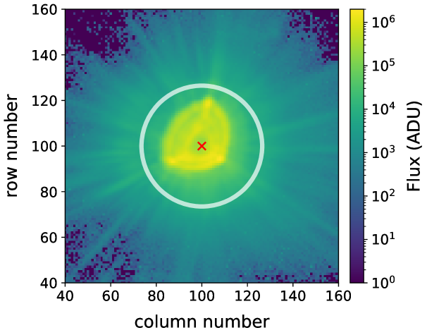
Figure 1: A CHEOPS exposure showing the typical PSF shape of the instrument, including the centroid of the star as determined by the DRP marked with a red cross and the OPTIMAL aperture being shown with a white circle.

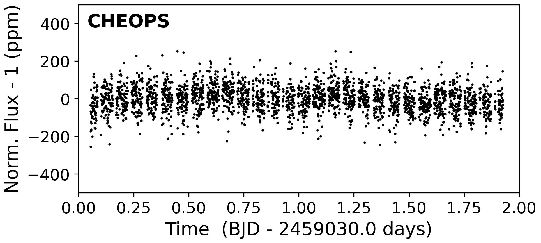
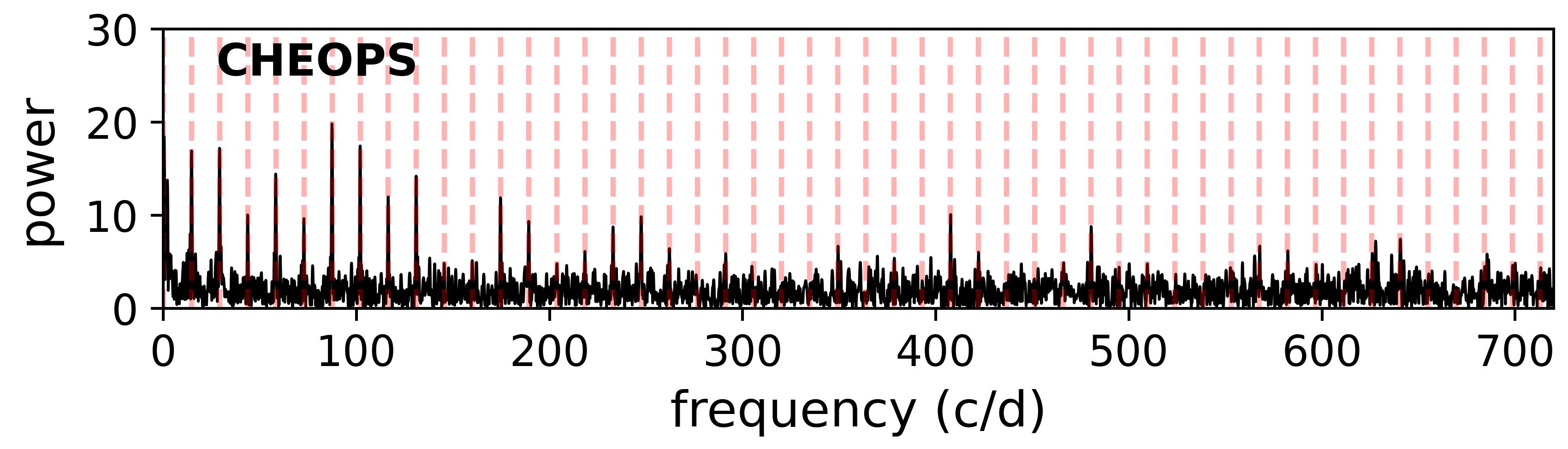
Figure 2: Top: Full CHEOPS lightcurve. Normalized and outliers removed. Bottom: Periodogram corresponding to CHEOPS data. Vertical red dashed lines shows peaks at multiples of 14.5 cpd ($\sim$ 100 minutes), corresponding to the orbital breaks of the satellite.

The CHEOPS (Benz et al., 2021) data were taken as part of program CH_PR210021 (“Hunting for exocomets transiting the young naked-eye star 5 Vulpeculae”, PI Rebollido) between June 29^th and July 01^st 2020 (see Table 2). Due to the objective of observing a non-periodic transit, the observations were targeted to be non-interrupted, and led to one visit over a duration of 44.96 hours. Data were processed with the latest version of the CHEOPS automatic Data Reduction Pipeline (DRP v13.1.0). The pipeline corrects the raw images (bias subtraction, gain conversion, flat fielding, dark correction and non-linearity) and then performs aperture photometry. An example for a CHEOPS exposure can be found in Fig. 1. A detailed description of DRP can be found in Hoyer et al. (2020). The pipeline outputs light curves with differently sized apertures: R = 25.0 pixels (DEFAULT), R = 22.5 pixels (RINF), R = 30.0 pixels (RSUP), and R = 26.5 (OPTIMAL). The latter maximizes the signal-to-noise ratio (SNR) of the photometry by maximizing the flux coming from the target while minimizing the flux from background stars. This SNR calculation, performed by the DRP, uses the Gaia catalogue and the PSF shape of CHEOPS. The OPTIMAL aperture has a resulting point-to-point root-mean-square (rms) of 63.9 ppm, which is the lowest of all considered apertures. We therefore chose the OPTIMAL aperture for our analysis. Figure 2, top pannel, shows the CHEOPS light curve used in this analysis. Flagged observations (which might indicate cosmic ray events or crossing of the South Atlantic Anomaly) and outliers greater than 4$\sigma$ with respect to the median have been removed. These make up approximately 4% of the total observations. The corresponding periodogram is shown in the bottom pannel of Fig. 2. The vertical dashed lines indicate the multiples of 14.5 cpd ($\sim$ 100 min), corresponding to the orbital breaks of the satellite. No other frequencies show significant peaks.

Table 2: Observations with TESS and CHEOPS used in this work.

Observation	Start Date (UTC)	End Date (UTC)	Exp. time (s)
TESSS14	2019-Jul-18 20:35:54	2019-Aug-14 16:59:19	120
TESSS40	2021-Jun-25 03:46:55	2021-Jul-23 08:35:25	120
TESSS54	2022-Jul-09 09:41:08	2022-Aug-04 15:11:01	120
CHEOPS	2020-Jun-29 13:16:11	2020-Jul-01 10:13:44	44

2.2.2 TESS

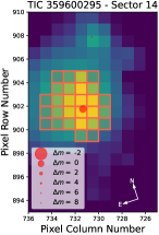
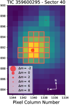
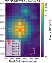
Figure 3: TESS target pixel files (TPFs) for 5 Vul in Sector 14, 40 and 54. The pixels shaded in red indicate the aperture used by the SPOC pipeline. There are no stars within the aperture of 5 Vul with a Gaia magnitude difference smaller than 8, meaning ackground stars do not significantly contribute to the measured flux of 5 Vul. Plot made using tpfplotter (Aller et al., 2020).

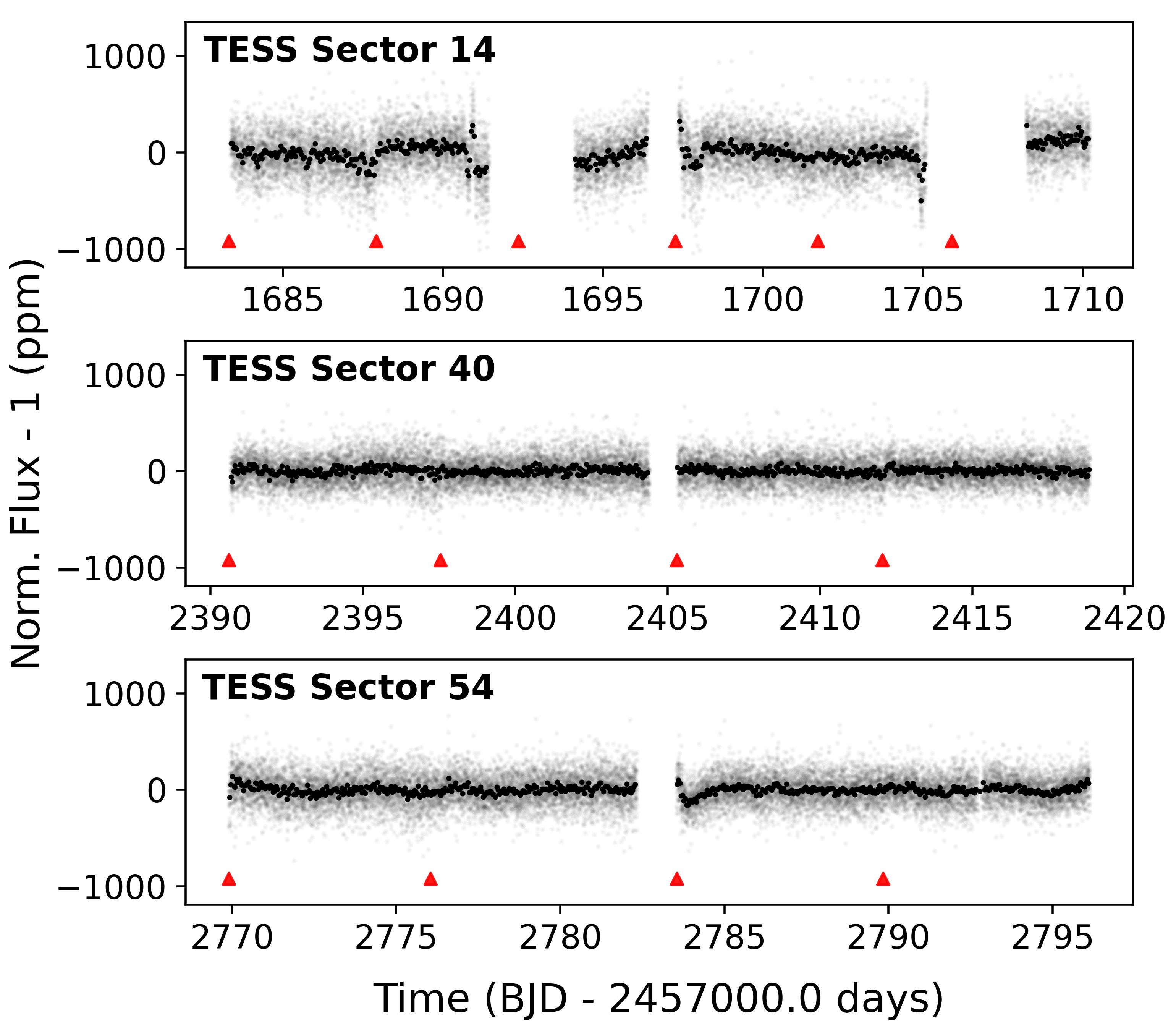
Figure 4: Full TESS lightcurve. Telescope momentum dumps are marked with red arrows. The 2-minute cadence TESS data (shown in light gray) have been binned to timescales of an hour for better visualisation.

5 Vul (TIC 359600295) was observed by TESS (Ricker et al., 2015) in Sector 14 from 2019 July 18 to 2019 August 14, in Sector 40 from 2021 June 25 to 2021 July 23 and in Sector 54 from 2022 July 09 to 2022 August 04 at a 2 minute cadence (see Table 2). Data were processed by the TESS Science Processing Operations Center (SPOC) pipeline (Jenkins et al., 2016) and accessed using the python package lightkurve (Lightkurve Collaboration et al., 2018) which downloads the data from the Mikulski Archive for Space Telescopes (MAST) archive. Target pixel files are shown in Fig. 3. For this analysis, we used the Pre-Search Data Conditioning Simple Aperture Photometry (PDCSAP; Smith et al., 2012; Stumpe et al., 2012; Stumpe et al., 2014) light curves. In contrast to the Simple Aperture Photometry (SAP) light curves, the PDCSAP data are corrected for instrumental systematic effects and show considerably less scatter and variability caused by instrumental events like momentum dumps. The PDCSAP light curves were flagged by the SPOC pipeline for bad data which mark anomalies like instrumental issues or cosmic ray events. We removed any TESS exposure in our dataset with a non-zero “quality” flag. For Sector 14, scattered light from the Earth was saturating the part of the detector where 5 Vul hit on silicon. We excluded these times which occurred in the last quarter of each orbit (see Fig. 4 around BTJD 1691-1694 and BTJD 1705-1708). The breaks of approximately one day in the middle of each Sector, are related to the data downlink of TESS when it reaches its perigee. Figure 4 shows that any significant changes in flux occur at the beginning or at the end of an TESS orbit or during momentum dumps and are therefore not caused by the star itself. In total, we removed approximately 7% of the TESS data mostly due to saturation of Camera 1 in Sector 14. Figure 3 shows the pointing of TESS in Sector 14, 40 and 54, showing that there are no close, bright stars nearby which could bias our flux measurements.

The TESS data do not show any significant periodic signals which could be attributed to stellar variability (see Figure 5). Systematic signals at very short periods, such as the orbit of TESS around Earth, with a period of 14 days can be hinted from Fig. 4.

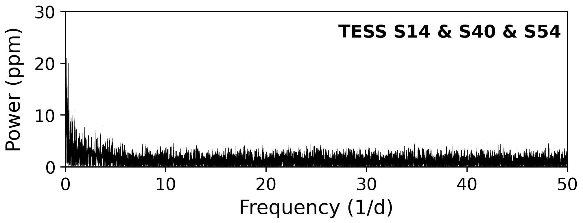
Figure 5: Lomb–Scargle periodogram of the full TESS lightcurve

3 Analysis of Results

There is no detection of flux fluctuations indicative of the presence of exocometary activity in the light curve of 5 Vul or any other transits with a significative depth (>5$\sigma$) after the analysis reported in Sec. 2.2. However, we can estimate comet sizes for a given trajectory based on the upper limits.

3.1 Detectability

Exocomets have been previously detected with Kepler (formally K2, Boyajian et al., 2016; Rappaport et al., 2018) and TESS (Zieba et al., 2019). While those missions were not designed for this particular science case, both have provided interesting results. The first detection of exocomets around a star with a spectral type different than A was in photometry, using K2 data (Rappaport et al., 2018), and the detection of photometric exocomets around $\beta$ Pic, the only star with exocomet detection using two different techniques, used TESS data (Zieba et al., 2019).

When compared to those missions, CHEOPS provides very similar capabilities. The cadence of CHEOPS observations is shorter (1 min), but comparable to TESS and Kepler (2 min). The photometric precision, however, is much better, with an estimated 10 ppm for a V=6 star against $\sim$ 50 ppm for TESS (Ricker et al., 2015) and while a number of bright targets were observed with Kepler (e.g. Guzik et al., 2016), the magnitude of 5 Vul exceeded Kepler’s nominal mission, and it was never observed. The response of the detectors is very unlikely to be responsible for detection rates either, since it is very similar to TESS and practically identical to Kepler .

Therefore, the non-detection in this target is most likely related to the lack of exocometary transits at the time of observations, as explained in Sect. 4.2, and not to the instrumental capabilities.

3.2 Maximum exocomet size

Given that there is previous evidence of exocomets in the system, we explore the range of sizes and periastrons that we are sensitive to. We propose two different approaches for the size estimation, and test them for the different detection limits of both observatories.

3.2.1 Estimation based on Hill spheres

Assuming exocomets have very eccentric orbits (Beust & Morbidelli, 2000), the more volatile materials evaporate as they come closer to the central star, developing a coma composed by the evaporating gas and the dust dragged by it. If we consider all the material in the coma to be optically thick and gravitationally bound to the nucleus, we can follow Boyajian et al. (2016) approximation, and estimate the maximum exocomet nucleus size we would be able to detect given the signal to noise ratio (SNR) of our lightcurve.

The depth of the transit, $\tau$, is directly related to the surface of the star covered by the comet, and for two spherical bodies can be expressed as a function of the ratio of their radius, $r$ and $R_{*}$ for the comet and star respectively,

$$\tau=\left(\frac{r}{R_{*}}\right)^{2}$$

Given our SNR, we would not be able to detect transits smaller than 5.85$\cdot$10^-3% (58 ppm) for TESS and 1.38$\cdot$10^-3% (13 ppm) for CHEOPS (see Figs. 2,4).

To retrieve the size of the comet associated to the clump, we can take into account the definition of Hill radius as:

$$R_{Hill}=a(1-e)~{}\left(\frac{M_{comet}}{3M_{*}}\right)^{1/3}$$

Given we are estimating all our material is optically thick, we can assume $\tau\sim R_{Hill}$. The minimum periastron values are limited by our cadence (1 min for CHEOPS and 2 min for TESS) following Kepler’s third law, and are consistent with the estimations for exocometary orbits for $\beta$ Pic (Lecavelier des Etangs et al., 2022). The obtained mass for the cometary nucleus can then be converted to radius considering a typical density for a comet of $\mathrm{0.5~{}g/cm^{3}}$ (Britt et al., 2006).

Fig. 6 shows in red the minimum size of the exocometary nucleus for an A0V star (2.193 R_⊙ and 2.18 M_⊙ Pecaut & Mamajek, 2013). From this calculation we can estimate that any body that transited the star during the observations must have had a nucleus smaller than $\sim$ 5.2 km for CHEOPS and $\sim$ 10.7 km for TESS at a distance of 1 AU. The fact that the increase in distance allows to trace smaller bodies is based on our first assumption of all material released in the evaporation process is contained in the Hill sphere and optically thick, which might not be a realistic approximation. Actually, assuming a similar composition throughout the system, the further from the star the exocomet is, the less material we are able to extract from the comet due to the inverse squared dependence of stellar flux with distance. Therefore, in the next section we explore a size estimation that contains evaporation models.

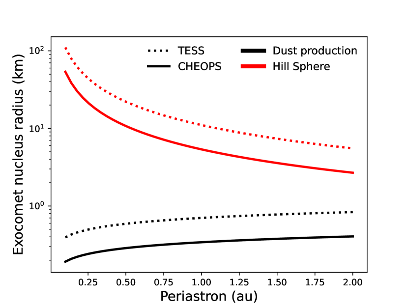
Figure 6: Minimum exocomet nucleus size estimates accessible with both CHEOPS (solid line) and TESS (dotted line) observations as a function of periastron distance. Red lines show size estimations for a spherical exocometary body with all the opaque material gravitationally bound to the central body (Hill sphere). Black lines show size estimations based on dust production rates.

3.2.2 Estimations based on dust production rates

Following the calculation made by Lecavelier des Etangs et al. (2022), we can estimate the corresponding minimum exocomet dust production rate that we would be able to detect with our lightcurves.

The typical absorption depth ($AD$) in a light curve that is caused by the transit of an exocomet is given by Lecavelier des Etangs et al. (2022):

$$AD=5\cdot 10^{-5}\left(\frac{\dot{M_{1{\rm au}}}}{10^{5}\,{\rm kg/s}}\right)\left(\frac{q}{1\,{\rm au}}\right)^{-1/2}\left(\frac{M_{\star}}{{\rm M}_{\sun}}\right),$$

where $\dot{M_{1{\rm au}}}$ is the comet dust production rate taken at 1 au from the star, $q$ is the comet orbit periastron distance, and $M_{\star}$ the mass of the star. Therefore a detection limit in absorption depth can be translated into a corresponding maximum dust production rate. For a stellar mass $M_{\star}$=2.18 M_⊙ (Pecaut & Mamajek, 2013), we obtain

$$\dot{M_{1{\rm au}}}=1.2\cdot 10^{4}\,{\rm kg/s}\left(\frac{AD}{13\,{\rm ppm}}\right)\left(\frac{q}{1\,{\rm au}}\right)^{1/2}$$

Recalling that the Hale-Bopp comet had a dust prodution rate in the order of $2\cdot 10^{6}$ kg/s at 1 au from the Sun, we see that the CHEOPS observations are very sensitive to small comets.

Similarly as done by Lecavelier des Etangs et al. (2022), the dust production rate can be converted into a corresponding radius of the cometary nucleus using the relationship:

$$\dot{M_{1{\rm au}}}=2\cdot 10^{6}\,{\rm kg/s}\left(\frac{R}{30\,{\rm km}}\right)^{2}\left(\frac{L_{\star}}{{\rm L}_{\sun}}\right),$$

where $R$ is the radius of the comet nucleus and $L_{\star}$ the stellar luminosity, and we are considering a typical cometary radius and dust production similar to Hale-Bopp (Jewitt & Matthews, 1999; Fernández et al., 1999). With a luminosity of about 40 L_☉ for the A0 star 5 Vul (Yoon et al., 2010), we finally have

$$R=0.36\,{\rm km}\left(\frac{AD}{13\,{\rm ppm}}\right)^{1/2}\left(\frac{q}{1\,{\rm au}}\right)^{1/4}.$$

When taking into account the evaporation models, it appears that the presented CHEOPS and TESS observations with no exocomet photometric transit detection allow us to exclude the transit of very small bodies (0.3 km for CHEOPS and 0.7 km for TESS) at 1 au over the observation period.

4 discussion

The detection of exocomets using photometric data has been restricted to a few systems so far. Contrary to what is observed in spectroscopy, where most comets are found around A-type stars (e.g. Rappaport et al., 2018; Kennedy et al., 2019), the detections in photometry do not seem to be restricted to a certain spectral type. In the following we discuss the properties of 5 Vulpeculae, and what might be the origin of the discrepancy of the spectroscopic and photometric data.

4.1 Disc and planets

A faint debris disc is located in the environment of 5 Vul. Chen et al. (2014) report significant excess for wavelengths longer than 24 $\mu$m corresponding to a faint and likely not very massive disc, specially when compared to other debris discs around A-type stars. They fit two components to the disc, with two different blackbody (BB) temperatures, being the most massive the colder component (10^-5 M_⊕), at a distance of 34 au and with a BB temperature of $\sim$ 100 K. More recently, Musso Barcucci et al. (2021) reported a detection of the disc in band L, and fitted a single BB at $\sim$23 au, with a temperature of $\sim$ 180 K. The main goal of that paper was to look for planetary companions, and they also report 5$\sigma$ mass limits for all the investigated stars, including 5 Vul. However, the precision achieved can only estimate an upper limit for our system of >20 M_J at distances shorter than 50 au, twice the mass of $\beta$ Pic b. Their analysis of the self-stirring mechanisms (see Fig. A4 in Musso Barcucci et al., 2021) indicate that the disc is not large enough to produce the observed dust, and possibly a perturber (planet, companion, binary star) is affecting the system dynamics. Matthews et al. (2018) also reported no planetary companions larger than 8 M_J at distances larger than 10 au based on SPHERE observations in H2 and H3. Despite having hot Ca ii gas detected, located very close to the star (see Fig. 8) and a known debris disc, there is no detection of cold gas in the outer regions of the system (see e.g. Marino et al., 2020, and references therein for an overview of CO gas around A-type stars). Rebollido et al. (2022) report an upper mass limit for the dust and CO content based on ALMA observations of $\sim$ 10^-3 and 10^-6 M_⊕ respectively, consistent with previous models (Kral et al., 2017). The age of 5 Vul, estimated around 200 Myr (Chen et al., 2014) could potentially explain the low fractional luminosity and the lack of CO gas due to a decrease in dynamical activity as the system settles.

4.2 Spectroscopic counterpart in 5 Vul

The investigation of the 5 Vul spectra has revealed the presence of exocomets, reported in Montgomery & Welsh (2012); Rebollido et al. (2020). We show in Fig. 7 spectra previously published in Rebollido et al. (2020) and publicly available online . The exocometary events were detected within -5 and 60 km/s in both cases, with one extra tentative detection located at -35 km/s. The poor time coverage does not allow for a follow up of the events. Moreover, both papers report variability of the more stable component (at $\sim$-20. km/s consistent with the radial velocity of the star, but also with the G interstellar cloud Redfield & Linsky, 2008), suggesting at least a partially circumstellar origin and variations in the amount of circumstellar gas.

There are 39 spectra in Rebollido et al. (2020) spanning 22 nights, which overall show variable absorptions both blue and red-shifted in approximately 20% of the observations. This is consistent with a frequency of one detected variation every 4.2 days. Montgomery & Welsh (2012) show one exocometary red-shifted absorption in 4 spectra, and small variations in the EW measurements of the stable feature that seem gradual with time (see Fig. 3 and Table 2 of Montgomery & Welsh, 2012), again consistent with variations in  20% of the observations.

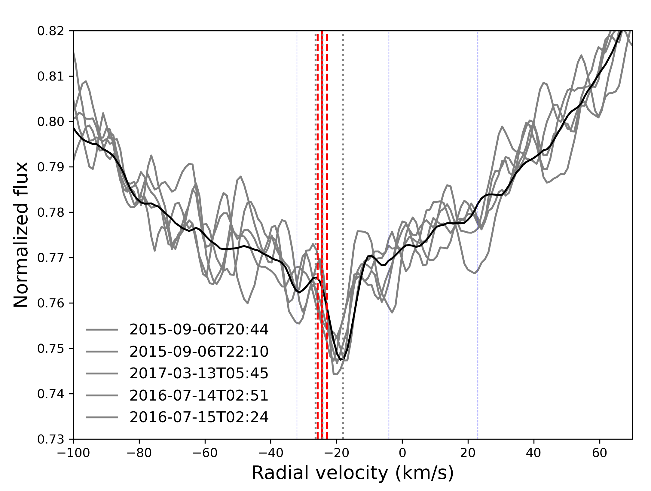
Figure 7: Spectroscopic evidence of exocomets in 5 Vul. Variations are seen at -3.5, 23 and -31 km/s, indicated by the blue vertical lines. Red vertical lines show the radial velocity of the object (-24.3 $\pm$ 1.4 km/s), and grey vertical lines show the radial velocity of the ISM in the line of sight (-18.05, -24.21, -26.30 km/s).

4.3 Photometric comets vs. Spectroscopic comets

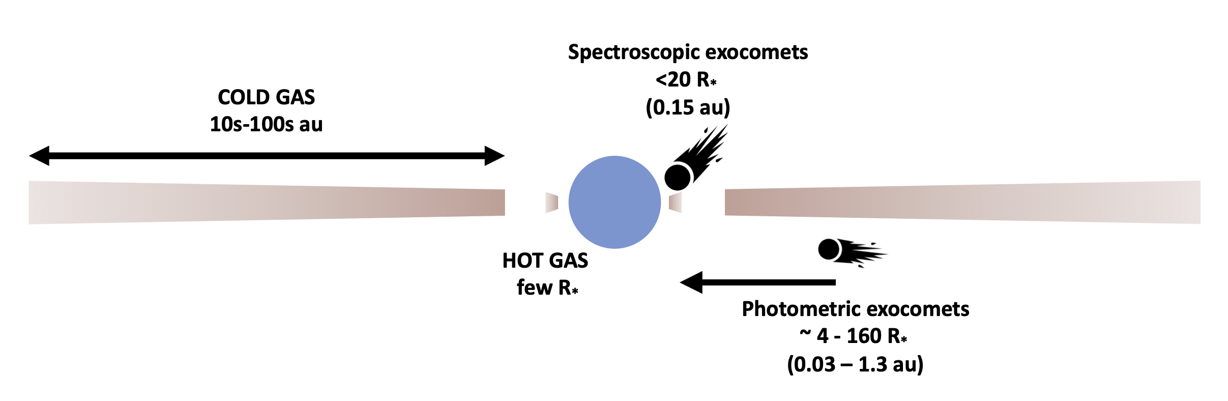
Figure 8: Estimated distribution of gas and exocometary bodies in a typical exocometary system.

The only star where exocomets have been found both in spectroscopy and photometry is $\beta$ Pic (Ferlet et al., 1987; Kiefer et al., 2014a; Zieba et al., 2019). The high frequency observed in spectroscopy, of around one exocometary absorption observed every hour to six hours, surpasses greatly any other exocomet host system (Kiefer et al., 2014a). However, the frequency of the photometric exocomets is much lower, with 30 events detected in 156 days through 4 different TESS sectors (Lecavelier des Etangs et al., 2022). The key to explain this discrepancy could be in the expected stellocentric distances traced by both techniques: while spectroscopic exocomets are expected to be located very close to the star (below 20R_∗, i.e. <0.15 au, Kiefer et al., 2014a; Kennedy, 2018), photometric ones are estimated at longer distances ($\sim$ 4-160 R_∗, i.e. 0.03 to 1.3 au; with an estimated average distance of 0.18 au, Lecavelier des Etangs et al., 2022). The question remains of whether different exocomet populations could be feeding different gas populations in the disc, i.e. gas detected in emission, much more extended (e.g. Marino et al., 2016; Matra et al., 2019; Rebollido et al., 2022; Kóspál et al., 2013; Moór et al., 2017, 2019) and hot gas detected in absorption, potentially released by exocomets and located closer to the star (e.g. Hobbs et al., 1985; Ferlet et al., 1987; Montgomery & Welsh, 2012; Iglesias et al., 2018, 2019; Rebollido et al., 2020). A diagram for the exocomet vs. gas location is shown Fig 8.

However, while the number of exocomets detected in spectroscopy remains larger than those detected in photometry, population D from Kiefer et al. (2014a) is more likely to be in better agreement with the orbital ranges of the photometric populations.

If we translate these exocomet ratios to the observed frequency around 5 Vul in spectroscopy, we would be expecting one photometric transit every 87.36 days, which would be hard to cover with current instrumentation and/or space missions.

5 Summary

Observations performed with CHEOPS and TESS of the star 5 Vulpecula show no evidence of exocometary activity in the lightcurve, despite the exocomet detection in spectroscopy around this star. In this work, we provided an estimation of the sizes and spatial location of the exocomets and a possible explanation for the non detection of exocometary transits via photometry.

The sporadic nature of exocomets makes it difficult to trace them, as their orbits are almost impossible to constrain. The few efforts to detect the dust counterpart of the exocomets observed in spectroscopy have only been successful for $\beta$ Pic. This is not surprising, given the high frequency of exocomets, so far much higher than any other. Even for $\beta$ Pic, only a handful of exocomets have been observed in photometry, contrasting the thousands of events that are reported in spectroscopy. This could potentially be related to the distance at which the exocomets evaporate/sublimate. The estimated distances for Ca ii production (where most exocomets have been detected) is just a few stellar radii, much closer to the estimated distances for the photometric observations. This could indicate we are probing two different groups of exocomets: star-grazing comets that sublimate refractory materials (i.e., calcium), and comets at larger orbits, where the cloud of dust is better sustained.

Lecavelier Des Etangs et al. (1999) estimated dozens of exocometary detections in photometry for large surveys with tens of thousands of stars in the worst case scenario. However, the results from large missions like Kepler and TESS show otherwise, with very few detections so far (e.g. Ansdell et al., 2019; Zieba et al., 2019; Boyajian et al., 2016). Given that as of today a large enough sample of stellar ages and spectral types have been observed, the number of detectable exocomets might have been overestimated based on the activity around $\beta$ Pic.

Data Availability

Data are available in the CHEOPS and TESS archives:
https://cheops-archive.astro.unige.ch/
https://archive.stsci.edu/missions-and-data/tess

References

- Aller et al. (2020) Aller A., Lillo-Box J., Jones D., Miranda L. F., Barceló Forteza S., 2020, A&A, 635, A128
- Ansdell et al. (2019) Ansdell M., et al., 2019, MNRAS, 483, 3579
- Benz et al. (2021) Benz W., et al., 2021, Experimental Astronomy, 51, 109
- Beust & Morbidelli (1996) Beust H., Morbidelli A., 1996, Icarus, 120, 358
- Beust & Morbidelli (2000) Beust H., Morbidelli A., 2000, Icarus, 143, 170
- Boyajian et al. (2016) Boyajian T. S., et al., 2016, MNRAS, 457, 3988
- Britt et al. (2006) Britt D. T., Consolmagno G. J., Merline W. J., 2006, in Mackwell S., Stansbery E., eds, 37th Annual Lunar and Planetary Science Conference. Lunar and Planetary Science Conference. p. 2214
- Chen et al. (2014) Chen C. H., Mittal T., Kuchner M., Forrest W. J., Lisse C. M., Manoj P., Sargent B. A., Watson D. M., 2014, ApJS, 211, 25
- Ferlet et al. (1987) Ferlet R., Hobbs L. M., Vidal-Madjar A., 1987, A&A, 185, 267
- Fernández et al. (1999) Fernández Y. R., et al., 1999, Icarus, 140, 205
- Gaia Collaboration et al. (2016) Gaia Collaboration et al., 2016, A&A, 595, A1
- Gaia Collaboration et al. (2018) Gaia Collaboration et al., 2018, A&A, 616, A1
- Grady et al. (2018) Grady C. A., Brown A., Welsh B., Roberge A., Kamp I., Rivière Marichalar P., 2018, AJ, 155, 242
- Guzik et al. (2016) Guzik J. A., et al., 2016, ApJ, 831, 17
- Hobbs et al. (1985) Hobbs L. M., Vidal-Madjar A., Ferlet R., Albert C. E., Gry C., 1985, ApJ, 293, L29
- Hoyer et al. (2020) Hoyer S., Guterman P., Demangeon O., Sousa S. G., Deleuil M., Meunier J. C., Benz W., 2020, A&A, 635, A24
- Iglesias et al. (2018) Iglesias D., et al., 2018, MNRAS, 480, 488
- Iglesias et al. (2019) Iglesias D. P., et al., 2019, MNRAS, 490, 5218
- Jenkins et al. (2016) Jenkins J. M., et al., 2016, in Chiozzi G., Guzman J. C., eds, Society of Photo-Optical Instrumentation Engineers (SPIE) Conference Series Vol. 9913, Software and Cyberinfrastructure for Astronomy IV. p. 99133E, doi:10.1117/12.2233418
- Jewitt & Matthews (1999) Jewitt D., Matthews H., 1999, AJ, 117, 1056
- Kennedy (2018) Kennedy G. M., 2018, MNRAS, 479, 1997
- Kennedy et al. (2019) Kennedy G. M., Hope G., Hodgkin S. T., Wyatt M. C., 2019, MNRAS, 482, 5587
- Kiefer et al. (2014a) Kiefer F., Lecavelier des Etangs A., Boissier J., Vidal-Madjar A., Beust H., Lagrange A. M., Hébrard G., Ferlet R., 2014a, Nature, 514, 462
- Kiefer et al. (2014b) Kiefer F., Lecavelier des Etangs A., Augereau J. C., Vidal-Madjar A., Lagrange A. M., Beust H., 2014b, A&A, 561, L10
- Kóspál et al. (2013) Kóspál Á., et al., 2013, ApJ, 776, 77
- Kral et al. (2017) Kral Q., Matrà L., Wyatt M. C., Kennedy G. M., 2017, MNRAS, 469, 521
- Lecavelier Des Etangs (1999) Lecavelier Des Etangs A., 1999, A&AS, 140, 15