Isotropic Point Cloud Meshing using unit Spheres (IPCMS)

Abstract

Point clouds arise from acquisition processes applied in various scenarios, such as reverse engineering, rapid prototyping, or cultural preservation. To run various simulations via, e.g., finite element methods, on the derived data, a mesh has to be created from it. In this paper, a meshing algorithm for point clouds is presented, which is based on a sphere covering of the underlying surface. The algorithm provides a mesh close to uniformity in terms of edge lengths and angles of its triangles. Additionally, theoretical results guarantee the output to be manifold, given suitable input and parameter choices. We present both the underlying theory, which provides suitable parameter bounds, as well as experiments showing that our algorithm can compete with widely used competitors in terms of quality of the output and timings.

1 Introduction

Point cloud meshing is an important topic present in different fields of research and in various applications. Examples include reverse engineering, see [11], where 3D scanning is employed to create data on designs that are lost, obsolete, or withheld. Meshes of these data are then used to recreate the original designs. In the case of rapid prototyping, e.g., within medical applications, see [5], meshes from point clouds are used for instance in the process of prosthesis and implant development. In cultural sectors, such as art or architecture, see [21], scans of artifacts and their respective meshes are used for restoration or reconstruction.

Since scanning real world objects is a mechanical procedure, difficulties may arise from the scanning process in terms of outliers, noisy data, or non-uniform samplings depending both on the scanner and on the scanned object itself. So far, established methods in the realm of denoising or outlier-removal aim for dealing with these issues, but are not necessarily tuned to output high-quality meshes. Aside from this, the output is not guaranteed to be manifold, as opposed to the scanned object’s surface. However, in many processing techniques manifoldness and high mesh quality are of utter importance.

Arguably one of the most important processing techniques on geometric models are finite element methods (FEM). First described in the 1940s, FEM are now ubiquitous in any simulation context from dynamical systems to material science, see [19]. Despite their powerful applications and many new developments in the field, the numerical properties of FEM remain sensitive to the quality of the underlying geometric representation. Often, numerical robustness can only be guaranteed—if possible at all—if both the mathematical simulation problem and the underlying geometric domain satisfy certain constraints.

Reducing to surface domains, i.e., to two-dimensional geometries embedded in three-dimensional space, the widest used geometric representation is a triangle mesh. A wide-spread proxy for the quality of these meshes is given by the distribution of the edge lengths that occur in the mesh. If the edges of the mesh are of a length close to uniformity, the triangles are almost equilateral, which is well-suited for simulations, e.g., via FEM. These triangulations are called isotropic, which differs from adaptive or anisotropic meshes. The latter vary the size of the triangles—and their edges—in order to obtain a memory-efficient representation of the geometry. We, however, aim to produce isotropic meshes, as their uniform edge length does not only provide high mesh quality, but also enables a whole set of applications, e.g., in fabrication. There, a large variety of building blocks is undesired and a mesh close to uniformity helps ease of construction as well as lowering costs.

In this publication, we consider point clouds that were created by scanning a real world model, the so-called ground truth, equipped with either a provided or a generated normal field, and aim for the reconstruction of the underlying geometry. The resulting mesh is created with special consideration of the triangle quality, as measured by an edge length close to uniformity across the mesh. The algorithm presented in this paper is based on a sphere-packing algorithm previously published, see [18]. It is extended such that, if the input and the given or estimated normals satisfy certain quality assumptions, the output of the algorithm is manifold.

The robustness of the algorithm as well as the quality of the resulting meshes will be illustrated with several experiments. Furthermore, the results are compared to standard algorithms in the field. In summary, the contributions of this paper are:

• presentation of a meshing algorithm that places touching spheres of uniform radius on the input,

• which creates edge lengths close to uniformity and of a guaranteed minimum length, i.e., high-quality triangles,

• as well as manifold output, provided a suitable input geometry and good enough normals.

2 Related Work

In the last decades, several attempts were made to reconstruct the ground truth from a given point cloud $\mathcal{P}$. The resulting reconstruction depends on the quality of the input $\mathcal{P}$, which might be accompanied by noise on the points as well as on their normals, outliers, or a non-uniform sampling. Different approaches have been made to overcome these challenges, which possibly lead to ruffled regions, non-covered areas, or changes in the topology. Furthermore, some algorithms tend to smooth out small features.

Established methods can be divided into two groups, creating interpolating and approximating meshes, respectively. The first group works on the given data itself while the second group uses the given points to compute new ones. On top of a reconstruction, the user may ask for guarantees such as correct topology [1], or convergence to the ground truth by increasing the sampling density [16]. Some algorithms guarantee local connectedness of their output [2], while others guarantee their output to stay within in the convex hull of the given input [9]. Other user requirements are, for instance, a result mesh of high quality, i.e., consisting of triangles of length close to uniformity and vertices of degree close to $6$, or low computational costs. For an overview of surface reconstruction algorithms, we refer to a recent surface reconstruction survey [13].

Here, we present in detail a selection of established algorithms deriving triangle meshes from a given point cloud. These algorithms serve as comparisons in our experiments, see Section 5, and were chosen for their wide use in the field as they are implemented in prominent geometry processing frameworks. Namely, we compare to Poisson surface reconstruction [14], advancing front reconstruction [7], and scale-space reconstruction [8]. These three algorithms are all implemented in the surface reconstruction pipeline of the Computational Geometry Algorithms Library (CGAL), see the tutorial on Surface Reconstruction from Point Clouds [10]. Additionally, we include Voronoi cell reconstruction [4] and a multi-grid Poisson reconstruction [15]. These two algorithms are available as part of the Geogram framework [17]. Finally, we employ the robust implicit moving least squares (RIMLS) surface reconstruction [23], which is available as part of the MeshLab software [6]. In the following paragraphs, we will provide a short overview of these algorithms.

First, we consider the technique based on a Poisson equation [14]. An implicit function framework is built where the reconstructed surface appears by extracting an appropriate isosurface. The output is smooth and robustly approximates noisy data. Additionally, densely sampled regions allow the reconstruction of sharp features while sparsely sampled regions are smoothly reconstructed. Later, these ideas are further developed to create watertight meshes fitting an oriented point cloud by using an adaptive, finite elements multi-grid solver capable of solving a linear system discretized over a spacial domain [15].

The scale-space approach [7] aims at topological correctness by carefully choosing triangles based on a confidence-based selection criterion. This avoids accumulation of errors, which is often detected in greedy approaches. The algorithm is interpolating, can handle sharp features to a certain extend, but does not come with proven topological correctness.

The advancing front algorithm [8] handles sets of unorganized points without normal information. It computes a normal field and meshes the complete point cloud directly which leads to a high-level reconstruction of details as well as to an accurate delineation of holes in the ground truth. Therefore, a smoothing operator consistent with the intrinsic heat equation is introduced. By construction, this approach is almost interpolating and features are preserved given very low levels of noise.

The robust implicit moving least squares (RIMLS) algorithm [23] combines implicit MLS with robust statistics. The MLS approach [16] is a widely used tool for functional approximation of irregular data. The development to RIMLS is based on a surface definition formulated in terms of linear kernel regression minimization using a robust objective function which gives a simple and technically sound implicit formulation of the surface. Thus, RIMLS can handle noisy data, outliers, and sparse sampling, and can reconstruct sharp features. The number of iterations needed to achieve a reliable result increases near sharp features while smooth regions only need a single iteration. Furthermore, RIMLS belongs to the set of algorithms producing approximating meshes.

Another approach for surface reconstruction is based on placing triangles with regard to the restricted Voronoi diagram of a filtered input point set [4]. This approach has the largest similarity to our algorithm, as we will also employ Voronoi diagrams, however, only to filter points on the tangent plane. Another shared aspect is that both this and our algorithm work on a set of disks centered at the input points, oriented orthogonal to a guessed or provided normal direction. Our approach exceeds this simple Voronoi approach in two aspects. As we base our surface reconstruction on a set of touching spheres placed on the underlying surface, we are able to provide certain theoretical guarantees on the output: given suitable input and parameter choices, our output is always manifold. Furthermore, the output of our algorithm has a guaranteed minimum edge length, while striving towards uniformity of occurring edge lengths.

Note that all these algorithms come with different guarantees regarding the output. Furthermore, they optimize various aspects of the surface reconstruction pipeline. A specific aspect that will be put special emphasis on in our method will be the distribution of edge lengths and the mesh being manifold given a suitable input and user-chosen parameters. In Section 5, we will provide a detailed comparison of our algorithm with the works listed here.

3 Methodic Overview

The goal of the algorithm is to reconstruct a manifold $\mathcal{M}$ with a triangle mesh whose edge lengths are close to uniformity and that is manifold from unstructered input. In Section 3.1, we first present some theoretical considerations that will form the basis for the practical realization of our approach to point cloud meshing as discussed in this paper. Subsequently, the relatively simple geometric idea is illustrated that enables us to compute the triangle mesh, see Section 3.2. This is followed by a detailed overview of the single steps of the presented algorithm in Sections 3.3 to 3.5. In an additional section, the used data structures are explained and reviewed with respect to efficiency and memory consumption, see Section 4. In that section, finally, we highlight the differences and additions of our approach to that of [18] and present the complete algorithm in form of pseudo code, see Section 4.5.

3.1 Theory

We first need to understand the necessary conditions on both the input and the parameters of the algorithm that have to be placed in order to achieve a corresponding manifold output. These conditions will be given as the results of the following theoretical considerations.

Let $\mathcal{M}$ be an orientable, compact $\mathcal{C}^{2}$-manifold embedded into $\mathbb{R}^{3}$, which is assumed to be closed and of finite reach ${\rho\coloneqq\inf\left\{\|a-m\|\mid a\in\mathcal{A}_{\mathcal{M}}\,\land\,m\in\mathcal{M}\right\}\in\mathbb{R}_{>0}}$, where $\mathcal{A}_{\mathcal{M}}$ is the medial axis  of $\mathcal{M}$ consisting of the points $q\in\mathbb{R}^{3}$ fulfilling $\min_{p\in\mathcal{M}}|q-p|=|q-\hat{p}|=|q-\tilde{p}|$ for $\hat{p}\neq\tilde{p}\in\mathcal{M}$.

On the manifold $\mathcal{M}$, we define the geodesic distance $d_{\mathcal{M}}$ as follows.

Definition 1.

Let ${\operatorname{len}(f)=\int_{0}^{1}\left|f^{\prime}(t)\right|\>dt}$ denote the length of a curve $f\in\mathcal{C}^{1}([0,1],\mathcal{M})$ in $\mathcal{M}$. Then the geodesic distance $d_{\mathcal{M}}$ of $m,m^{\prime}\in\mathcal{M}$ is defined as $\inf\left\{\operatorname{len}(f)\mid f\in\mathcal{C}^{1}([0,1],\mathcal{M}):f(0)=m\land f(1)=m^{\prime}\right\}$.

In Lemma 3 in [3], the authors state that for any $p,q\in\mathcal{M}$ such that $\|p-q\|<2\rho$, the following estimation holds:

$$\|p-q\|\leq d_{\mathcal{M}}(p,q)\leq 2\rho\arcsin\left(\frac{\|p-q\|}{2\rho}\right).$$ (1)

Let $T_{p}\mathcal{M}$ and $T_{q}\mathcal{M}$ denote the tangent planes at ${p,q\in\mathcal{M}}$. Lemma 6 in [3] gives an upper bound for the angle $\sphericalangle\left(T_{p}\mathcal{M},T_{q}\mathcal{M}\right)$ between them,

$$\sphericalangle\left(T_{p}\mathcal{M},T_{q}\mathcal{M}\right)\leq\frac{d_{\mathcal{M}}(p,q)}{\rho}.$$ (2)

Hence, Inequalities (1) and (2) imply for the normal vectors $N_{p}$ at $p$ and $N_{q}$ at $q$ that

$$\begin{split}&\varphi\coloneqq\sphericalangle\left(N_{p},N_{q}\right)\leq 2\arcsin\left(\frac{\|p-q\|}{2\rho}\right)\\ \Rightarrow&\|p-q\|\geq r(\varphi)\coloneqq 2\rho\sin\left(\frac{\varphi}{2}\right).\end{split}$$ (3)

For a given angle $\varphi_{\max}\in\left[0,\tfrac{\pi}{2}\right[$, the second part of Equation (3) implies that there is a constant $r_{\max}\in\mathbb{R}_{\geq 0}$ such that $\varphi\leq\varphi_{\max}$ if $\|p-q\|<r_{\max}$. Denote by $\mathcal{M}^{\prime}\coloneqq B_{r_{\max}}(p)\cap\mathcal{M}$ the part of $\mathcal{M}$ that is contained in $\mathcal{M}$ and the ball $B_{r_{\max}}(p)$ centered at $p$. Then, the normals $N_{q}$ of all points $q\in B_{r_{\max}}$ have positive Euclidean scalar product with $N_{p}$. The assumption that $\mathcal{M}$ is of positive finite reach guarantees that $\mathcal{M}^{\prime}$ is a single connected component. Hence, $\mathcal{M}^{\prime}$ has a parallel projection to the tangent plane $T_{p}\mathcal{M}$ without over-folds. Additionally, the following lemma holds.

Lemma 1.

Let $p\in\mathcal{M}$ be a point and let $N_{p}$ denote its normal. Then, for $r<\rho$, the image of $B_{r}(p)\cap\mathcal{M}$ under the projection $\pi$ in direction of $N_{p}$ to the tangent plane $T_{p}\mathcal{M}$ is a convex set.

Proof.

Corollary 1 from [3] states that the intersection $\mathcal{I}$ of a closed set $\mathcal{S}\subset\mathbb{R}^{d}$ having reach $\rho_{\mathcal{S}}>0$ with a closed ball $B_{r}(x)$, $r<\rho_{\mathcal{S}}$ and $x\in\mathbb{R}^{d}$, is geodesically convex in $\mathcal{S}$. That is, the shortest path between any two points in $\mathcal{I}$ lies itself in the intersection. Furthermore, by Proposition 1 in [3], the intersection $\mathcal{M}^{\prime}$ of $B_{r_{\max}}$ and $\mathcal{M}$ is a topological disk as established above.

In the given scenario, $\mathcal{I}$ is not empty and consists of a surface patch since $p$ lies on $\mathcal{M}$. Hence, the boundary $\partial\mathcal{M}^{\prime}$ can be parameterized by a closed curve $\gamma$. Since $\mathcal{I}$ is geodesically convex, $\gamma$ has positive geodesic curvature. The inner product of the normals $N_{p}$ at $p$ and $N_{q}$ at an arbitrarily chosen point $q\in\partial\mathcal{I}$ is positive: $\langle N_{p},N_{q}\rangle>0$, by choice of $r$. Therefore, under projection along $N_{p}$ to the tangent plane $T_{p}\mathcal{M}$, the sign of curvature is preserved. Hence, the projection $\pi(\gamma)$ is a convex curve. ∎

(a) Splats of radius $s$.

(b) Projection to $T_{p}\mathcal{M}$.

(c) Voronoi cells in $T_{p}\mathcal{M}$.

(d) Individual splat radii.

Figure 1: Illustration of uniform splat sizes (1(a)), as well as the projection of a point $p$ and its neighborhood to the tangent plane $T_{p}\mathcal{M}$ (1(b)) and the Voronoi cells there with the farthest point circled (1(c)), which leads to individual splat sizes (1(d)).

Assume there is a graph $\mathcal{G}$ embedded on $\mathcal{M}$ and vertices in $\mathcal{G}$ connected by an edge have Euclidean distance $d$. The connected components remaining after removing $\mathcal{G}$ from $\mathcal{M}$ are called regions, denoted by $\mathcal{R}$. The set of vertices and edges incident to a region $R\in\mathcal{R}$ is called its border, denoted by $\partial R$. Note that because $\mathcal{M}$ is closed, each edge of $\mathcal{G}$ belongs to the border of exactly two regions. Also, each vertex of $\mathcal{G}$ can belong to the borders of several regions at once. Fix one such region $R\in\mathcal{R}$. Lemma 1 implies a choice of points $q_{1},\dotsc,q_{k}\in\partial R$ is mapped to points $\pi(q_{1}),\dotsc,\pi(q_{k})\in T_{p}\mathcal{M}$ in cyclic order, for $p\in R$ arbitrarily chosen. Hence, the regions can be extracted correctly (w.r.t. their topology) from the cyclic order of the edges at each vertex from the local projection. Given that the reach criterion is satisfied and given a suitable normal field, we can thus reconstruct a manifold from the input surface. In the following section, we will take these theoretical considerations into account when describing our algorithm.

(a) Connecting $v$ by two edges to the same border.

(b) Connecting $v$ to two different borders.

Figure 2: Possibilities when creating new vertices and edge connections in the graph: In 2(a), the new vertex $v$ and its two edges connect elements of the same border. Here, $v$ is created either in the in- or the outside region of the border. In 2(b), the new vertex $v$ is connecting two borders. After introducing $v$ and its edges, the respective outside regions are still connected, then $v$ and its edges join the borders. However, if the outside regions are split by $v$ and its edges, new borders are created which induce the corresponding regions.

3.2 Methodology

We assume to be given unstructered input in form of a point cloud ${\mathcal{P}=\{p_{i}\mid i=1,\ldots,n\}\subset\mathbb{R}^{3}}$ with corresponding normals ${\mathcal{N}=\{N_{p_{i}}\mid i=1,\ldots,n\}\subset\mathbb{S}^{2}}$ as input. Furthermore, we assume that $\mathcal{P}$ is sampling an underlying, possibly itself unknown manifold $\mathcal{M}$ with the properties as listed above. For point clouds with reach $0$, the output might not be manifold. To prevent non-manifold output, additional sanity checks are introduced.

Remark.

In the following discussion of the algorithm, we will refer to elements of the input point cloud $\mathcal{P}$ as points and to entities created by the algorithm as vertices.

Aside from the input point cloud $\mathcal{P}$, the user specifies two mandatory parameters: a target edge length $d$ as well as an initial splat size $s$. The former defines virtual spheres of radius $d/2$ around the vertices of the resulting mesh that are non-overlapping. Hence, all edges in the result mesh will have a minimum length of $d$. Following Lemma 1, the user has to choose the parameter $d$ with respect to the reach of the input, which can be estimated for point clouds [12], to ensure a manifold output.

For a point $p$ and its normal $N_{p}$, the second parameter defines the radius $s$ of a disk $S_{p}$ with normal $N_{p}$, centered at $p$, called a splat, see Figure 1(a). The parameter $s$ should be chosen sufficiently large for the splats to cover the surface, i.e., to be able to place vertices everywhere. Here, a geometry is said to be covered, if the union of projections of splats to the ground truth covers it. Then, we perform the following steps, which will be elaborated on in Sections 3.3 to 3.5.

1. Input: a point cloud $\mathcal{P}$, its normals $\mathcal{N}$, and the user-chosen parameters $d$ and $s$. Furthermore, the algorithm uses a maximum border length $\partial_{\max}$, see Section 3.5, and a window size parameter $w$, see Section 4.2.

2. The user initializes the algorithm by two starting vertices lying sufficiently close to each other such that a new vertex with distance $d$ to both can be placed on the splats.

3. Iteratively, place a new vertex on a splat such that it has distance $d$ to two currently existing ones, called parent vertices, and distance $\geq d$ to all other existing vertices. Stop when no additional sphere of radius $d/2$ can be added without intersecting any $d/2$-spheres around existing mesh vertices. After the disk-growing finished, all edges of the mesh have length $d$ by construction: Each time we add a new vertex $v$, we also insert two edges of length $d$ into the graph $\mathcal{G}$, connecting $v$ to its parent vertices. The edges will build a set of regions $\mathcal{R}$ of an (on average) short border length, representing the surface.

4. Finally, to obtain a triangulation, all regions $R\in\mathcal{R}$ are triangulated.

5. Output: a (manifold) triangulation $\mathcal{T}$ of $\mathcal{M}$.

3.3 Initialization

The user provides two starting vertices to initialize the algorithm. These vertices do not have to be points from the input $\mathcal{P}$, nor do they have to lie on the splats. After projecting the starting vertices to their closest splats, they form an initial vertex set of a graph $\mathcal{G}$. At this stage, $\mathcal{G}$ does not contain any edges. The starting vertices have to be chosen in such a way that their projections allow for placing a next vertex on a splat that is exactly distance $d$ away from two of them. These positions are the vertex candidates for next vertex placements.

3.4 Disk Growing to Create Graph and Regions

After initialization, disk growing is performed to create further vertices and edges of $\mathcal{G}$. Adding edges to $\mathcal{G}$ also changes the regions: By inserting a new vertex and its two edges, either one region border is split into two borders—see Figure 2(a)—or two borders join into a single one—see Figure 2(b).

As depicted in Figure 3, there might be regions having comparably long borders. These lead to visible seams in $\mathcal{G}$ as well as in the triangulation of $\mathcal{G}$. To avoid such seams in the final graph, we prioritize joining borders over splitting borders. Among possible splits, we want to prioritize splits with a bigger combinatorial distance between the parent vertices along the border over those with smaller distances.

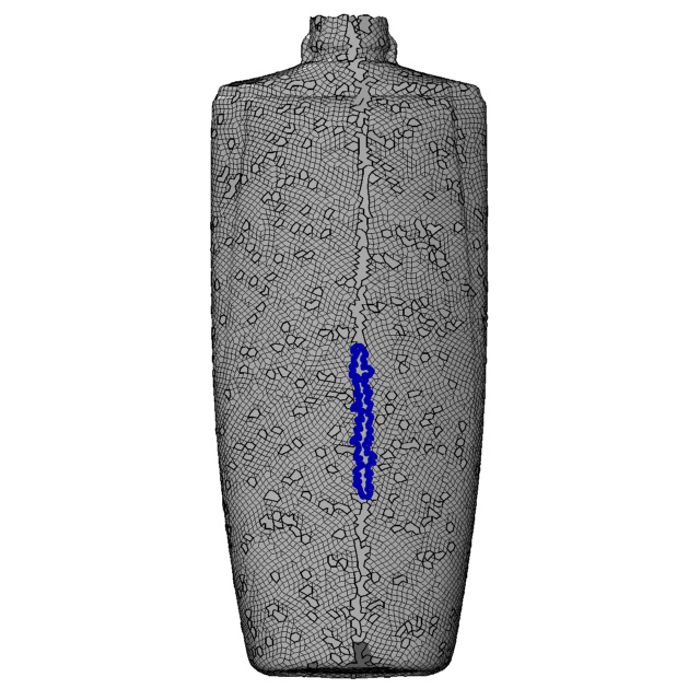
(a) Region of longest border length 93.

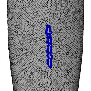
(b) Close-up of longest border length 93.

(c) Triangulated regions.

(d) Close-up of triangulated seam.

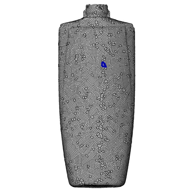
(e) Region of longest border length $11$.

(f) Close-up of longest border length $11$.

Figure 3: Appearance of visible seams on the Bottle Shampoo model. In 3(a) to 3(d), experimental results are shown achieved by inserting new vertices via pure breadth-first-growing. The seams appear as regions having a high number of border edges compared to all other regions on the surface. In 3(e) and 3(f), experimental results achieved by prioritizing new vertex candidates are shown. For better visibility, the target edge length  $d$ was chosen as $1$.

The disk growing process includes three stages: prioritization of vertex candidates, creation of new vertices from the candidate set, and creation of new vertex candidates. We will discuss each in the following.

(a) Border of length 0.

(b) Border of length 2.

(c) Border of length $k+1$.

Figure 4: Different borders and their respective regions: Border of length $0$ consisting of a single vertex and associated to a single, white, surrounding region (4(a)); border of length $4$, going back and forth between $v$ and $v^{\prime}$, associated to a single, white, surrounding region (4(b)); cycle of $k+1$ edges, separating the surface into an inner, light gray and outer, white region (4(c)).

3.4.1 Prioritizing of Vertex Candidates

A vertex candidate $v_{c}$ is chosen to become a vertex of $\mathcal{G}$ according to the following priorities, given in decreasing order:

1. At least one of the parent vertices has no edges incident to it. (Note: This parent vertex has to be a starting vertex from the initialization.)

2. At least one of the parent vertices is a vertex with only one edge incident to it.

3. Inserting $v_{c}$ and its two edges joins two borders.

4. Inserting $v_{c}$ splits a border—prioritize larger distance between parents along the common border.

In all cases, ties are broken by the breadth first strategy. To determine the priority of the vertex candidate to be added, it is necessary to know to which of the parent vertices’ borders the edges to be introduced will connect. To find the corresponding border, the candidate edge is projected to the plane defined by parent vertex and its normal. Note that because of the properties listed and the derivations given in Section 3.1, such a projection is possible without over-folds.

3.4.2 Creating a new Vertex

Once a vertex candidate $v_{c}$ has been chosen, it is first determined whether there is a vertex $v$ in the graph such that $\left\|v_{c}-v\right\|_{2}<d$. If so, the vertex candidate is discarded.

Next, the priority of $v_{c}$ is checked. In case the vertex does not satisfy the given priority anymore—e.g., because it was originally created with a parent vertex without any edges incident to it, but the parent vertex gained an edge by now—the vertex candidate’s priority is reduced and another vertex candidate is chosen.

Adding $v_{c}$ and the corresponding edges to $\mathcal{G}$ bears one additional problem. In practice, we do not always know whether the point cloud $\mathcal{P}$ fulfills the criteria listed in Section 3.1. If they are satisfied, the output is guaranteed to be manifold. However, the user might have chosen $d$ too large or the input point cloud might not sample a manifold in the first place. In either of these cases, all edges created from new vertices still have an edge length of $d$, but the edges might create non-manifold connections. Consider Figures 5(a) and 5(b) for an example of a surface with reach $\rho=0$, i.e., a surface violating the assumptions from Section 3.1. In these cases, we still want to prevent such faulty connections. Therefore, we choose a plane spanned by an approximated surface normal, see Section 4.1 for details. We project $v_{c}$ and its prospective edges as well as all edges already existing in the vicinity to $v_{c}$ onto this plane. For this projection, the vicinity of $v_{c}$ is bounded by $d$ in normal direction. We discard $v_{c}$ if either of its edges crosses an already existing edge, see Figure 5(b). While the algorithm creates manifold output for suitable input point clouds and choices of $d$, this mechanism improves the output even outside of this regime. If $v_{c}$ has passed these checks, itself and the two edges connecting it to its parent vertices are added to $\mathcal{G}$.

(a) 3D view of a tent-like feature, a geometry with reach $\rho=0$.

(b) Projection of the graph along an
approximated surface normal.

(c) The circle $c$; its intersection with splat $S$ gives the next vertex candidate.

Figure 5: An input geometry with a vertex candidate $v_{c}$ for insertion, edges to parent vertices are shown dotted (5(a)); the region projection shows an illegal edge crossing (5(b)). Illustration of the computation of vertex candidate positions (5(c)).

3.4.3 Computation of new Vertex Candidates

Once a new vertex $v_{\text{new}}$ is added, it can be used as parent vertex for new vertex candidates. For each splat $S$ intersecting a ball of radius $d$ centered at $v_{\text{new}}$ and for each vertex $v$ having Euclidean distance $\leq d$ to $S$, we compute the set of all points in the embedding space that have distance $d$ to $v$ and $v_{\text{new}}$. If $\left\|v_{\text{new}}-v\right\|_{2}<2d$, this is a circle $c$, see Figure 5(c). If $c$ intersects $S$, the intersection points are new vertex candidates, having $v$ and $v_{\text{new}}$ as parent vertices. To compute candidate positions, we solely have to solve a quadratic equation.

To iterate the disk growing, the steps described in Sections 3.4.2 and 3.4.3 are repeated until no further vertex candidate is left. The resulting graph is then exactly the graph described at the end of Section 3.1 and given a suitable input $\mathcal{P}$ and an suitably chosen $d$, it satisfies the properties listed there. This graph will now be used to build a triangle mesh.

3.5 Triangulating the resulting Regions

After the disk growing process has finished, the graph $\mathcal{G}$ provides a set of regions $\mathcal{R}$. On average, each vertex of $\mathcal{G}$ is connected to approximately four other vertices, see [18, 4.2]. Therefore, the average border length is approximately four. Hence, we are left with the task of triangulating these regions. Here, we give the user the choice to specify a maximal border length $\partial_{\max}$ that will leave the region as a hole rather than triangulating it. The reported results will use $\partial_{\max}=40$.

A region can be irregular in the sense that the inner angle of two consecutive edges can be bigger than $180^{\circ}$. In such cases, a projection of a single region to a plane is not necessarily a convex polygon. These inner angles of the faces are found by projecting the edges onto a plane given by the vertex normal. Then, we triangulate each region by iteratively cutting away the smallest angle as this leads to triangles close to equilateral ones.

4 Implementation

In this section, we will discuss an algorithmic implementation of the methodology presented above. This contains the introduction of data structures for efficient access as well as a discussion of the algorithm’s complexity. As stated in the beginning of Section 3.2, we assume to be given a point cloud $\mathcal{P}$, its normal field $\mathcal{N}$, user-chosen parameters $d$ and $s$ as well as algorithmic parameters $\partial_{\max}$ and $w$ (for the latter, see Section 4.2). If $\mathcal{P}$ does not come with a normal field, the user has to estimate one, e.g., via [22].

4.1 Box Grid Data Structure

When introducing new vertex candidates, see Section 3.4.3, we need to know all splats close to a given, newly introduced vertex. In order to have access to these, we build a box grid data structure consisting of equal-sized, cubical boxes of side-length $d$ partitioning the three-dimensional embedding space. Each box holds a pointer to those input points and their splats that are at most $d$ away, see Figure 6(c). This collection of points associated with box $b_{j}$ is denoted by $\mathcal{B}_{j}$.

As preliminary filter step, we compute an average normal $\overline{N}_{b_{j}}$ for each box $b_{j}$ by summing up the normals of all those points that $b_{j}$ has a pointer to, without normalizing the sum. If $\left\|\overline{N}_{b_{j}}\right\|_{2}$ is smaller than $0.1$, we keep all points in $b_{j}$. If the length is at least $0.1$, we can assume that enough points agree on a normal direction in this box. Then, we remove those points $p$ from the box for which $\langle N_{p},\overline{N}_{b_{j}}\rangle<0$. We choose a value of $0.1$ for the length check to filter a small number of points while maintaining coherent normal information. This will ensure that the following step can succeed.

(a) Adding a new vertex.

(b) Collecting splats (top view).

(c) Collecting splats.

(d) Finding candidates.

Figure 6: Adding new vertex (6(a)); associating splats to a box $b$ (6(b)); collecting normals (6(c)); finding positions for new vertex candidates (6(d)).

For each box $b_{j}$ with at least one associated splat, we compute a box normal $N_{b_{j}}$. It will be used for projection steps that will ensure manifold properties of the resulting mesh. This will provide approximated surface normals that allow us to work on data which do not fulfill the requirements listed in Section 3.1, such as the example shown in Figure 5(a). To compute an approximation efficiently, we take a finite sampling $\mathcal{S}_{F}\subset\mathbb{S}^{2}$ and derive the box normal $N_{b_{j}}$ as

$$N_{b_{j}}=\operatorname*{arg\,max}_{N\in\mathcal{S}_{F}}\min_{p_{i}\in\mathcal{B}_{j}}\langle N_{p_{i}},N\rangle\approx\operatorname*{arg\,max}_{N\in\mathbb{S}^{2}}\min_{p_{i}\in\mathcal{B}_{j}}\langle N_{p_{i}},N\rangle.$$

That is, we search for the unit normal that maximizes the smallest scalar product with all point normals associated to the box $b_{j}$. For each box $b_{j}$, the scalar product $\langle N_{p_{i}},N_{b_{j}}\rangle$ is ideally strictly positive for all points $p_{i}\in\mathcal{B}_{j}$, even in those cases where we did not filter the normals. Therefore, it allows for a projection onto a plane spanned by $N_{b_{j}}$ as normal vector such that all points remain positively oriented by their normals. The newly computed box normal is also used as vertex normal for all vertices lying in $b_{j}$ from now on.

To achieve a fast lookup, we can either build a uniform grid on the complete bounding box of the input or create a hash structure to only store those boxes that are including input points from $\mathcal{P}$. The uniform grid has faster access, but results in many empty boxes and thus large memory consumption. The hash structure does not use as much memory, but the access is slower. In our experiments, we utilize the hash structure to be more memory efficient.

Note that in Section 3.2, we stated that for creating new vertex candidates, we need to traverse all splats that are distance $d$ away from a given point. However, here we are collecting all splats that are at distance $\leq d$ from the box, thus possibly resulting in a higher number of splats to be considered. That insures that the spheres from Section 3.2 are inscribed into the volume within $d$-distances around the boxes, see Figure 6(b).

This leads to the question how to choose a good side-length of the boxes. As stated above, we use side-length $d$, i.e., their size coincides with the target edge length for the triangulation. For smaller values, each splat would be associated to more boxes, hence the memory demand would grow. For larger boxes, there will be many splats associated to each box that do not actually lead to vertex candidates with the currently considered vertex. Thus, the runtime would grow when checking all splats being far away from the currently considered vertex. Finally, for larger boxes, it will also become more difficult to compute a suitable box normal for projections. Hence, we advocate for the middle ground and choose $d$ as the box size.

Note that the last observation regarding the box normals lead to a heuristic how to check the user’s parameter choice of $d$. Namely, a choice of $d$ is considered too large if there is a box whose box normal has negative scalar product with any point normal of a point registered in the box. This provides a mechanism to alert the user that they have chosen the parameter $d$ outside of the specifications as provided in Section 3.1 and that the output is thus not guaranteed to be manifold anymore.

4.2 Window Size

During the disk growing process, we maintain a data structure representing the region borders. They consist of oriented half-edge cycles. Note that this includes degenerate cases, such as a single vertex, which we interpret as a border of length $0$, see Figure 4(a). Each time a new vertex and the two edges to its parent vertices are added to $\mathcal{G}$, this creates four new half-edges which have to be linked to the existing borders. To avoid tracing very long distances along the borders, we introduce a window size $w$ after which the tracing is stopped. A window then consists of $2w+1$ vertices on a common border, running in both directions centered at the vertex currently considered.

Recall the split and join operation from Section 3.4. Note that by cutting the tracing at a finite window size, it is not longer possible to distinguish between a split and join operation in all cases. However, preliminary experiments showed that windows sizes of ${w\geq 8}$ all produced the same quality output, despite not distinguishing splits or joins.

Furthermore, we experienced that setting the window size to ${w=0}$ immediately creates noticeable negative effects on the result of the algorithm. In this case, our algorithm defaults to the breadth-first strategy of [18] and thus creates visible seams on the geometry, see Figures 3(a) to 3(d). Starting from window sizes of ${w=2}$ or ${w=3}$, benefits in the quality of the output are apparent as larger visible seams are prevented. On the one hand, theoretically, a larger window size will increase the lookup time. Therefore, in our implementation of the algorithm, we go for ${w=8}$ as a large enough window size to reap its benefits, but a small enough one to not impact the algorithm’s run time.

4.3 Discussion of Splat Size

In case of non-uniform sampling density, using a global splat size $s$ might lead to areas covered multiple times. For more densely sampled areas, a smaller splat size guarantees the creation of vertices closer to the sampling points. In our preliminary experiments, we saw that in high-curvature regions, smaller splats have small deviation from the surface, while larger splats deviate from the surface significantly. Hence, when looking for vertex candidates on large splats, the algorithm can place vertices that are somewhat distant to the input points, see Figure 7. Therefore, we turn to individual, smaller splat sizes to reduce the deviation of the vertices with respect to an underlying surface represented by the input point cloud.

(a) Result with uniform splat sizes.

(b) Result with individual splat sizes.

Figure 7: Result of our algorithm on the Bowl Chinese model from [13]. The result 7(a) is obtained with global splat sizes. In particular on the rim of the bowl, the curvature is high and the splats are far away from the underlying geometry. This leads to noticeable artifacts that are remedied by smaller, local splat sizes, as seen in 7(b).

An additional benefit is that for smaller splat sizes, there are less splats registered per box, which speeds up the algorithm. However, the individual splats have to have sizes sufficient to cover the underlying geometry. To find the specific splat size $s_{p}$ for each point ${p\in\mathcal{P}}$, we use the box data structure, see Figure 1(d). Namely, we consider all points $p_{i}$ associated to the box containing $p$. To map the points $\{p_{i}\}$ to $T_{p}\mathcal{M}$, consider the plane $N_{\perp}$ containing $p$ and $p_{i}$ and being perpendicular to $T_{p}\mathcal{M}$. For each $p_{i}$, an auxiliary point $\pi(p_{i})$ is determined by rotating $p_{i}$ around $p$ around the smaller angle in $N_{\perp}$ until it lies in $T_{p}\mathcal{M}$. Hence, $p$ and $\pi(p_{i})$ have the same distance $d_{i}$ as $p$ and $p_{i}$ have. Based on a cyclic sorting around $p$, we compute a central triangulation, connecting all projections to $p$ and connecting them pairwise according to their angular sorting, see Figure 1(b). For the resulting triangulation, we test whether or not we can flip a central edge to make the incident triangles Delaunay. Points $p_{i}$, whose edges are flipped, are removed from the following consideration. For those neighboring points that remain, consider the Voronoi diagram of their triangulation. We choose the local splat size $s_{p}$ as distance from $p$ to the farthest Voronoi vertex, see Figure 1(c). This ensures that all Delaunay triangles are still completely covered. By choosing local splat sizes in this way, the visible deviation from the underlying geometry is reduced, see Figure 7.

4.4 Processing Vertex Candidates

The processing of vertex candidates, following Section 3.4 consists of the following steps: popping a vertex candidate from the priority queue, checking feasibility of the candidate, adding a suitable candidate as well as its edges to $\mathcal{G}$, and adding new vertex candidates to the priority queue.

Note that because of the window size, there is a finite number of priorities, as given in Section 3.4.1. Each of these priorities is handled via its own queue that follows a strict first-in-first-out strategy. Hence, getting a candidate from the priority queue runs in constant time.

If a vertex still has correct priority, checking for conflict with existing vertices and performing the projection check from Figure 5 both requires access to nearby vertices. This is a constant-time operation because of the box data structure that holds all relevant vertices. Furthermore, the number of vertices within distance $2d$ is, by construction, bounded from above by the densest sphere packing in space, which is a constant.

Once a new vertex $v_{\text{new}}$ is created, we compute new vertex candidates having $v_{\text{new}}$ as parent vertex. Therefore, we need the set of all splats intersecting the ball of radius $d$ centered at $v_{\text{new}}$. This is a subset of the set of those splats associated to the box containing $v_{\text{new}}$. To efficiently access potential second parent vertices, we maintain for each splat $S$ a list of all vertices within distance $d$ to $S$, see Figures 6(b) and 6(c).

4.5 Pseudo Code and Comparison to previous Work

Having presented the methodology of the algorithm in Section 3.2 and implementation details in Section 4, we summarize the steps of our algorithm in the following pseudo code segment.

Algorithm 1 Isotropic Point Cloud Meshing using unit Spheres

point cloud $\mathcal{P}$, normal field $\mathcal{N}$, target edge length $d$, splat size $s$, starting vertices $q,q^{\prime}$, window size $w$, maximum border length $\partial_{\max}$

triangle mesh $\mathcal{T}$ with edge lengths close to uniformity

 

Build box grid, register splats in all boxes up to distance $d$ (possibly with individual splat sizes), filter points according to the average normal, compute box normals.

Project $q$ and $q^{\prime}$ to their closest splats, start a graph $\mathcal{G}$ by adding the projections as vertices.

Compute initial vertex candidates and their priority, add candidates to the queue.

while candidate vertex $v_{c}$ exists in the queue do

     if $\mathcal{G}$ has vertex $v$ s.t. $\left\|v-v_{c}\right\|_{2}<d$ or $v_{c}$ fails the projection check then

         Discard $v_{c}$.

     else if priority of $v$ is not correct then

         Correct priority by pushing $v_{c}$ back to the queue.

     else

         Add $v_{c}$ and edges to its parent vertices to $\mathcal{G}$, update region borders. Compute new vertex candidates around $v_{c}$ and their priorities, add them to the queue.      

for each region $R\in\mathcal{R}$ do

     while length of region border $\partial R$ is $\geq 3$ and $<\partial_{\max}$ do

         Cut triangle $t$ at the smallest border angle, add $t$ to $\mathcal{T}$.      

While the algorithm of [18] was an inspiration for the method presented here, there are several noteworthy differences and improvements. First, we introduce the box grid data structure that not only provides fast access, but also serves as a means to compute the newly introduced box normals. The introduction of window sizes speeds up the priority lookup significantly, reducing it from the length of the border to a predetermined constant. Additionally, we extended the algorithm to work on splats, so that it can handle unorganized point sets instead of meshes. Finally, the new projection check makes the algorithm more robust and ensures the output to be almost manifold even in the cases where the theoretical bounds of Section 3.1 do not hold.

5 Experimental Results

Having introduced the algorithm and its implementation, in this section, we present several qualitative and quantitative experiments on and around the presented method. We compare the output of our algorithm to several widely used surface reconstruction algorithms. Here, we show that our algorithm can compete with these both with respect to the quality of the obtained triangle meshes as well as the time to compute the output.

In our experiments, we focus on the reconstruction of real-world scan data. For this, we turn to 20 scanned objects provided as part of a surface reconstruction benchmark [13]. Here, we concentrate on high-resolution scans obtained by an OKIO 5M scanning device, resulting in 330k to 2,000k points per surface after 20 shots. The shots are registered and do come with a normal field. All data sets are publicly available, see the repository of [13]. Out of the 20 point clouds, we used 19 as they are provided in the repository. One model, the scan of a remote control, had a clear registration artifact. Here, one of the buttons of the remote was registered into the remote, i.e., was not pointing up, but down. This, we corrected manually by removing the wrongly registered points.

On these data, we perform surface reconstruction and aim for a high-quality triangulation with a uniform edge length of $0.2$, measured in absolute world units. We measure the quality of the obtained triangulations as follows: For a triangle $t\in\mathcal{T}$ with edge lengths ${\ell_{1}(t),\ell_{2}(t),\ell_{3}(t)}$ and area $A(t)$, following [20], we compute the quality $Q(t)$, its average $Q_{\text{avg}}$, and the root mean square deviation in percent $Q_{\text{RMS}}$ as:

$$Q(t)=\frac{4\sqrt{3}A(t)}{\ell_{1}(t)^{2}+\ell_{2}(t)^{2}+\ell_{3}(t)^{2}},$$

$$Q_{\text{avg}}=\frac{1}{|\mathcal{T}|}\sum_{t\in\mathcal{T}}Q(t),$$

$$Q_{\text{RMS}}=\frac{100}{Q_{\text{avg}}}\sqrt{\frac{1}{|\mathcal{T}|}\sum_{t\in\mathcal{T}}\left(Q(t)-Q_{\text{avg}}\right)^{2}}.$$

See Section 3 of [24] for a relation of this quality measure to the stiffness matrix. Note that the factors normalize this quality metric to be $1$ for equilateral triangles and close to $0$ for very narrow slivers. Furthermore, from the set of all edges in the triangulation, we consider the average edge length $E_{\text{avg}}$ as well as the corresponding root mean square deviation $E_{\text{RMS}}$, also in percent.

As stated in Section 2, we will compare our algorithm to advancing front [7], Poisson [14], multigrid Poisson [15], RIMLS [23], scale space [8], and Voronoi surface reconstruction [4]. Poisson, advancing front, and scale space are run with the standard parameters as implemented in CGAL [10] except for the cleaning steps, which were unnecessary because of the high-quality input. Multigrid Poisson and Voronoi reconstruction are run with the standard parameters as implemented in Geogram [17]. RIMLS is run with the standard parameters from Meshlab [6], using a smoothness of 2 and a grid resolution of 1000.

Note that we aim for an algorithm that provides high-quality triangulations out-of-the-box, right after reconstruction. However, as the comparison algorithms do not necessarily optimize for a uniform edge length, we take their respective results and process them with the “Isotropic Explicit Remeshing” filter of Meshlab. This filter repeatedly applies edge flip, collapse, relax, and refine operations. We run 3 iterations with a target edge length of $0.2$ in absolute world units for the input of [13]. In Tables 1 to 4, we report both the results of the comparison algorithms and the result after these have been remeshed, indicated by “(Re)”.

These tables include some representative models, a full report with data for all 20 models can be found in the supplementary material. We chose the Bottle Shampoo and the Bowl Chinese model because of their features, as explored in Figures 10(a) to 10(h) and 7. The Toy Bear model has several differently curved parts, which makes it ideal for an investigation of varying starting points, Figure 9. Finally, the Cloth Duck is one of two models from the repository where the competing methods had the largest gain on our algorithm when measured by $E_{avg}$ (the other is the Mug model, see supplementary material).

Algorithm	$|\mathcal{T}|$	$E_{\text{avg}}$	$E_{\text{RMS}}$	$Q_{\text{avg}}$	$Q_{\text{RMS}}$
Adv. Front	1.209,546	0.1799	39.6	0.8247	16.0
Adv. Front (Re)	928,850	0.2028	15.3	0.9416	6.1
Poisson	16,280	1.2946	74.8	0.8760	12.3
Poisson (Re)	498,140	0.2657	38.6	0.9251	7.5
Poisson MG	150,770	0.5318	35.7	0.7204	33.7
Poisson MG (Re)	952,830	0.2015	16.3	0.9330	7.0
RIMLS	1,907,781	0.1499	35.8	0.7055	35.1
RIMLS (Re)	1,054,438	0.1905	19.3	0.9117	11.5
Scale Space	1,209,093	0.1798	39.1	0.8248	16.0
Scale Space (Re)	926,828	0.2028	15.2	0.9417	6.0
Voronoi	1,209,792	0.1799	52.3	0.8241	16.1
Voronoi (Re)	923,476	0.2044	20.8	0.9407	6.8
Ours	840,453	0.2131	11.2	0.9577	4.5
Ours (Re)	854,257	0.2098	10.4	0.9701	3.8

Table 1: Experimental results on the Bottle Shampoo (604,903 input points).

Algorithm	$|\mathcal{T}|$	$E_{\text{avg}}$	$E_{\text{RMS}}$	$Q_{\text{avg}}$	$Q_{\text{RMS}}$
Adv. Front	1,212,636	0.2920	38.2	0.8045	18.6
Adv. Front (Re)	2,407,002	0.2038	15.4	0.9405	6.2
Poisson	13,584	2.3850	63.2	0.8845	11.7
Poisson (Re)	637,488	0.3732	40.8	0.9301	6.9
Poisson MG	503,458	0.4710	39.8	0.7062	37.1
Poisson MG (Re)	2,409,076	0.2050	17.7	0.9223	7.9
RIMLS	6,458,589	0.1331	40.4	0.6877	39.6
RIMLS (Re)	2,441,143	0.2023	15.4	0.9394	6.3
Scale Space	1,093,339	0.2779	34.9	0.8054	18.7
Scale Space (Re)	1,947,592	0.2006	16.1	0.9351	7.3
Voronoi	1,212,636	0.2916	38.4	0.8042	18.7
Voronoi (Re)	2,398,584	0.2039	15.3	0.9405	6.1
Ours	2,137,650	0.2167	14.8	0.9485	6.2
Ours (Re)	2,246,434	0.2093	11.4	0.9665	4.3

Table 2: Experimental results on the Bowl Chinese (606,320 input points).

Algorithm	$|\mathcal{T}|$	$E_{\text{avg}}$	$E_{\text{RMS}}$	$Q_{\text{avg}}$	$Q_{\text{RMS}}$
Adv. Front	2,037,574	0.1839	40.1	0.8143	17.3
Adv. Front (Re)	1,739,214	0.1965	19.4	0.9179	9.5
Poisson	147,940	0.6300	44.3	0.8805	12.0
Poisson (Re)	1,488,112	0.2068	17.5	0.9311	7.2
Poisson MG	419,614	0.4086	38.5	0.7160	36.0
Poisson MG (Re)	1,463,018	0.2093	18.7	0.9154	8.8
RIMLS	5,878,521	0.1154	39.9	0.6919	38.9
RIMLS (Re)	1,728,371	0.1978	20.1	0.9143	12.7
Scale Space	2,036,816	0.1839	40.0	0.8139	17.4
Scale Space (Re)	1,735,814	0.1965	19.3	0.9179	9.5
Voronoi	2,037,270	0.1767	41.8	0.8067	18.1
Voronoi (Re)	1,514,160	0.2027	15.4	0.9407	6.3
Ours	1,435,604	0.2181	15.7	0.9454	6.6
Ours (Re)	1,535,058	0.2089	12.5	0.9592	4.8

Table 3: Experimental results on the Cloth Duck (1,018,891 input points).

A first thing to notice when regarding the results presented in Tables 1 to 4 is that our algorithm achieves the best, i.e., highest values for $Q_{\text{avg}}$ on all models. This holds consistently across all 20 models from the repository. That is, our method produces the highest quality meshes, even when compared with the remeshed results of the other algorithms. For comparison, we also add the remeshed version of our algorithm, which generally improves the quality metrics slightly while destroying the minimum edge length guarantee. Note again that the goal of this paper is not to compare different remeshing approaches, but to present a method that can provide high-quality triangle meshes right after reconstruction, without remeshing, hence the remeshed version of our algorithm is set apart in gray and only carries bold font if it causes an improvement on the previously best result. In this setting, the comparison to the remeshed results just serves to place our results in a broader setting.

Algorithm	$|\mathcal{T}|$	$E_{\text{avg}}$	$E_{\text{RMS}}$	$Q_{\text{avg}}$	$Q_{\text{RMS}}$
Adv. Front	1,214,998	0.1474	36.3	0.8474	13.9
Adv. Front (Re)	629,138	0.2024	15.2	0.9418	6.0
Poisson	20,134	1.0381	54.7	0.8882	11.7
Poisson (Re)	530,374	0.2193	22.8	0.9293	7.3
Poisson MG	432,268	0.2585	39.5	0.2623	37.1
Poisson MG (Re)	629,508	0.2021	15.0	0.9436	6.1
RIMLS	5,548,226	0.0730	40.0	0.6910	39.3
RIMLS (Re)	618,531	0.2049	16.2	0.9322	6.8
Scale Space	1,214,990	0.1474	36.3	0.8474	13.9
Scale Space (Re)	628,848	0.2025	15.2	0.9417	6.0
Voronoi	1,214,996	0.1471	36.5	0.8471	13.9
Voronoi (Re)	616,160	0.2041	15.0	0.9427	5.9
Ours	555,490	0.2159	13.5	0.9499	5.6
Ours (Re)	578,730	0.2096	11.5	0.9657	4.3

Table 4: Experimental results on the Toy Bear (607,501 input points).

On most of the models, the deviation $Q_{\text{RMS}}$ has also the lowest percentages for our algorithm. Notable exceptions are the Bowl Chinese model, Table 2, and the Cloth Duck model, Table 3. However, across all models, the lowest deviation $Q_{\text{RMS}}$ is at most $0.6\%$ better than ours, cf. supplementary material.

Regarding the second metric, note that by construction, all edges produced by our algorithm are of length $\geq 0.2$. Therefore, the average edge length is also always greater than $0.2$, which places the remeshed output of other methods in the lead regarding the metric $E_{\text{avg}}$. However, the largest average edge length across all models is $0.2181$ for our algorithm, attained on the Cloth Duck model, Table 3, which is still very close to the target edge length.

Also, for almost all models, the width of the distribution of edge lengths, measured by $E_{\text{RMS}}$, is the lowest for our algorithm. That is, the triangulations produced are almost uniform. As a final observation regarding the quality metrics, note that those comparison algorithms that provide better metrics on the models do so only after an additional remeshing step. This shows that our algorithm does attain the goal of providing high-quality meshes immediately after reconstruction as it beats all comparison algorithms in this regard.

When inspecting the models visually, it is clear that, at least after remeshing, the triangulations are of high quality, see Figure 10. Note how some algorithms are not able to reproduce small details—e.g., a number 14 on the Bottle Shampoo model. Even in the remeshed version, line-like artifacts are still visible for some of the comparison algorithms. Our algorithm creates a mesh close to uniformity while retaining the details.

This uniformity can easily be observed by plotting histograms on the distribution of angles, edge lengths, and quality measures for a triangulation obtained by our algorithm. See Figure 8 for a corresponding set of plots for the Bottle Shampoo model and find histograms for the other models in the supplementary material. The histogram confirms that the triangle angles are centered around $60^{\circ}$, indicating a strong tendency towards equilateral triangles. Furthermore, we see that the edge lengths are indeed starting from the set minimum of 0.2 and that most edges actually attain this value. Finally, the histogram of the triangle quality reveals that there are many equilateral triangles (corresponding to a quality value of ${Q(t)=1}$) and that the distribution is skewed towards this highest quality value.

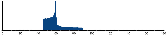
(a) Angle distribution, target=$60^{\circ}$.

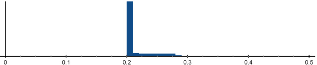
(b) Edge lengths distribution, target=0.2.

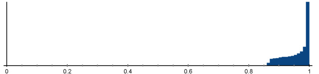
(c) Distribution of quality $Q(t)$, target=1.0.

Figure 8: Distributions on the triangulation of the Bottle Shampoo model as obtained by our algorithm (without remeshing).

Further experiments showed that the output is not sensitive to the choice of starting vertices, see Figure 9. For the eight resulting triangle meshes, the average edge length varies from $0.2158$ to $0.2159$, as does the average quality: from $0.9499$ to $0.9504$. In all cases, $E_{\text{RMS}}$ is equal to $13.5$ while $Q_{\text{RMS}}$ equals $5.6$.

Figure 9: Experiments with various starting vertices. From left to right: Toy Bear model with placements positions for starting vertex pairs, close up for pairs 1 to 8. The close ups show the area at one eye emphasized in the first image.

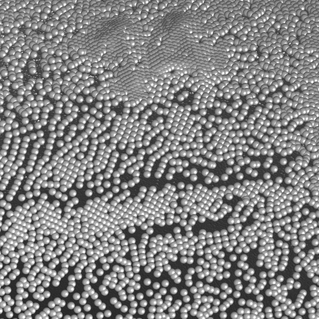
(a) Input Points.

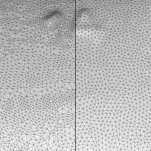
(b) Adv. Front.

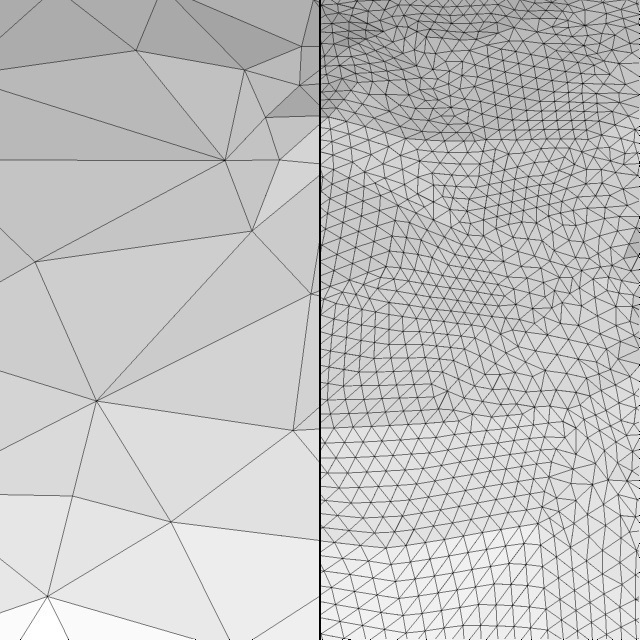
(c) Poisson.

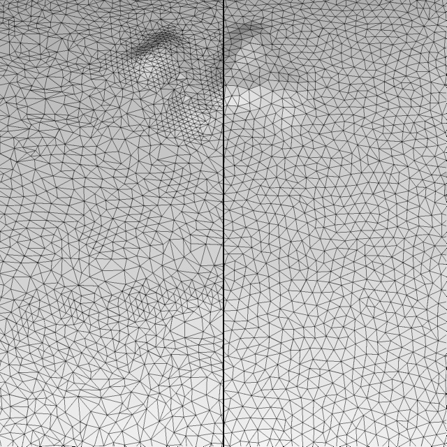
(d) Scale Space.

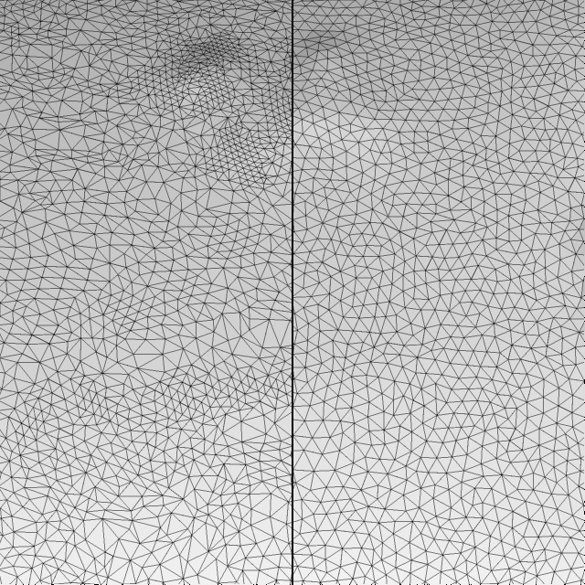
(e) Co3ne.

(f) Poisson MG.

(g) RIMLS.

(h) Ours.

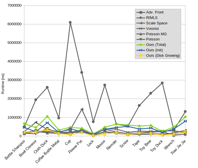
(i) Runtime of the algorithms on several models. Ours is additionally split into initialization and disk growing.

Figure 10: Qualitative comparison (10(b)–10(h)) without remeshing (left) and with remeshing (right). Comparison of the run times (10(i)).

Note that unlike some of the other algorithms and the remeshing step, our algorithm does not need iterations, but produces the output in a single sweep over the input. All experiments were run on a machine with an Intel(R) Core(TM) i7-5600U CPU 2.60GHz with four cores. Run times for several models are given in Figure 10(i), where the other algorithms are reported including the remeshing time. Note that our algorithm performs similar to most of the competitors.

Finally, we turn to the reconstruction quality of our algorithm. As the models discussed so far are real-world scans, there is no ground truth to compare the reconstruction with. For a simple experiment, we turn to two models that satisfies all assumptions made in Section 3.1 and that have an explicit mathematical parametrization to evaluate the reconstruction: the unit-sphere and a torus parametrized as a unit circle swept around a circle of radius 2 in the $xy$-plane. We sample both models uniformly, the sphere with 10,000 and the torus with 60,000 points, resulting in a similar density on the models. See Figures 11 and 12 for both the number of vertices created and the norm of these vertices. The norm is a direct measure for the reconstruction quality: For the sphere model, vertices with norm $1$ lie directly on the sampled sphere. For the torus model, we measure the norm as the distance to the circle in the $xy$-plane, i.e., a vertex with norm $1$ lies directly on the sampled torus.

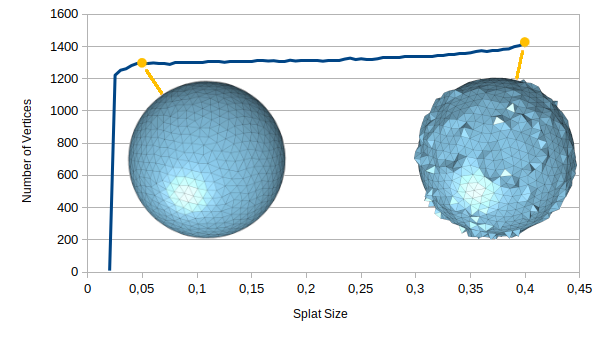
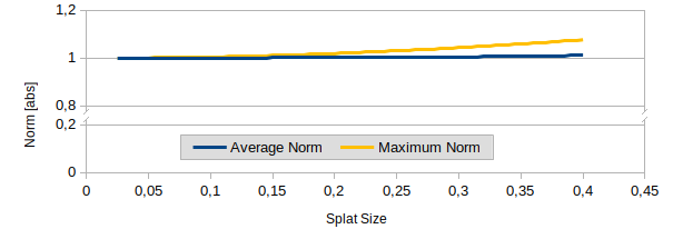
Figure 11: Measuring the reconstruction quality on the unit sphere.

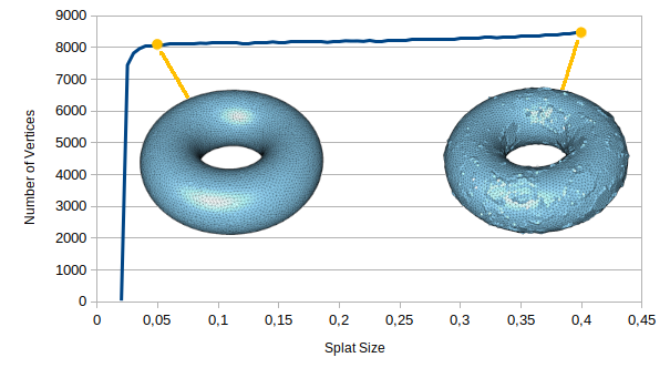
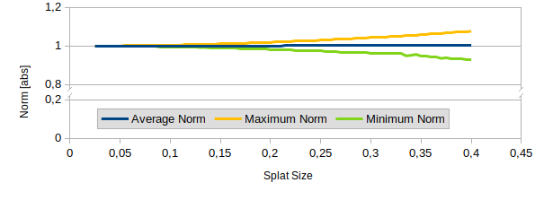
Figure 12: Measuring the reconstruction quality on a torus.

Note that for both models, the sphere and the torus, for too small splat sizes, the algorithm fails to cover the entire model. Hence, a very small number of spheres is created. Once a splat size is reached for which the entire model is covered, both the number of vertices and the reconstruction quality, measured by the norm, are very stable until larger splat sizes are reached, which cause visible distortion in the reconstructed models, see the added examples in Figures 11 and 12. This shows that for suitable splat sizes, large enough to cover the geometry, but as small as possible, our algorithm achieves close to optimal reconstruction results. To further highlight this, Figures 11 and 12 include the maximum and minimum norms. Note that for the sphere model, all points created are on or outside the sphere, placing the minimum at $1$. On the torus models, points are lying both in- and outside of the torus. Finally, note that even for the largest splat sizes of $0.4$ which create visible reconstruction artifacts, the reconstructed models are still manifolds, in line with our guarantees as laid out in Section 3.1.

6 Conclusion and Future Work

We have presented a surface reconstruction algorithm that produces triangulations with edge length close to uniformity, oriented at a user-chosen target edge length. In experiments with real-world scanned models, the algorithm can compete with several established state-of-the-art methods in both quantitative and qualitative aspects. Our implementation also proved to be competitive in a timed comparison.

The algorithm has the potential to be extended into different directions. First, choosing a large sphere diameter $d$ bears the potential of not only reconstructing the input in a coarser fashion, but also simultaneously smoothing out certain levels of noise that the input possesses. Second, introducing not two, but more starting vertices can be used for feature preservation. For instance, placing starting vertices in high-curvature regions will ensure that sampled features remain under the reconstruction. Finally, the algorithm can easily be altered to run on a mesh as input, where it can both create a manifold and simultaneously perform a remeshing. These extensions are left as future work.

Appendix A Supplementary Material

In this supplementary material, we present results of the algorithm introduced in our submission, applied to the complete set of twenty models as provided by the authors of [13]. See Figure 13 for a all models.

The experiments run on said repository are subdivided into two sections. In Section 4.2, we investigate the window size $w$ by running the algorithm on the Bottle Shampoo model with varying values for $w$. This motivates our standard parameter choice $w=8$ as presented in the paper. In Section A.2, we present results for each model. This includes:

• an image of the meshed model, as obtained by our algorithm,

• histograms showing the angle distribution, edge lengths distribution, and distribution of the triangle quality $Q(t)$ for the model,

• and the number of triangles and aggregated quality measures in tables.

See Section 5 of the paper for an explanation of these quantities. Note that the images and histograms displayed in Section A.2 come from the output of our algorithm without applying a remeshing step. As in the paper, the best values achieved for the root mean square deviation $E_{\text{RMS}}$, for the quality $Q(t)$ its average $Q_{\text{avg}}$, and the root mean square deviation $Q_{\text{RMS}}$ per model are highlighted. The table also shows values for a remeshed version of our results for comparison. Values are highlighted here if they improve those shown above.

Note that our algorithm produces a triangulation of edge lengths close to uniformity. This is reflected in the second histogram presented for each model, i.e., in the edge lengths distribution. The target edge length for all models is $0.2$, which—by construction—is also the lowest edge length possible in the output of our algorithm. Larger edges are possible, but there is a significant spike at the target edge length $0.2$. This insurance of a minimal edge length is the main reason why our algorithm does not perform best, but very close to best among the compared algorithms, when comparing average edge lengths in Tables 1 to 4 of the main paper. Because of the strict minimum at 0.2, there are no shorter edges that can bring the average closer to 0.2 again, cf. the discussion in Section 5 of the paper.

As the edges are all of very uniform length, the triangles are almost equilateral. This is noticeable by the large spike at $60^{\circ}$ in the first histogram of each model, showing the angle distribution.

Finally, note that a significant number of triangles $t$ of the resulting triangulations actually achieve very high up to highest quality possible, i.e., ${0.99<Q(t)=1}$, and are thus sorted into the last bin of the respective histogram. The distribution of this quality is very tight across all models. See Section 5 of the paper for the definition of this quality measure.

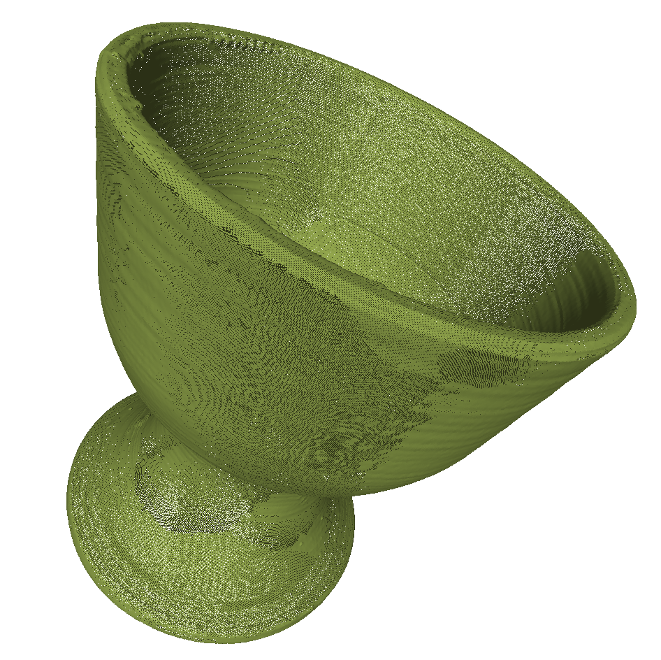
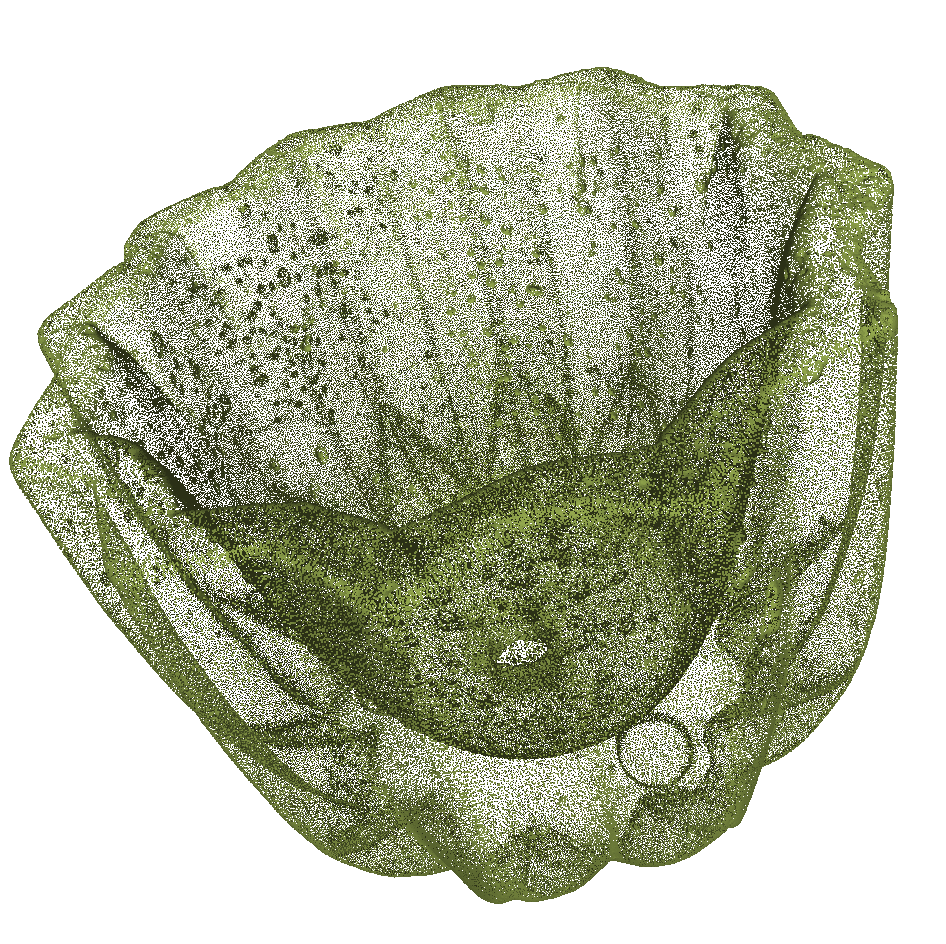
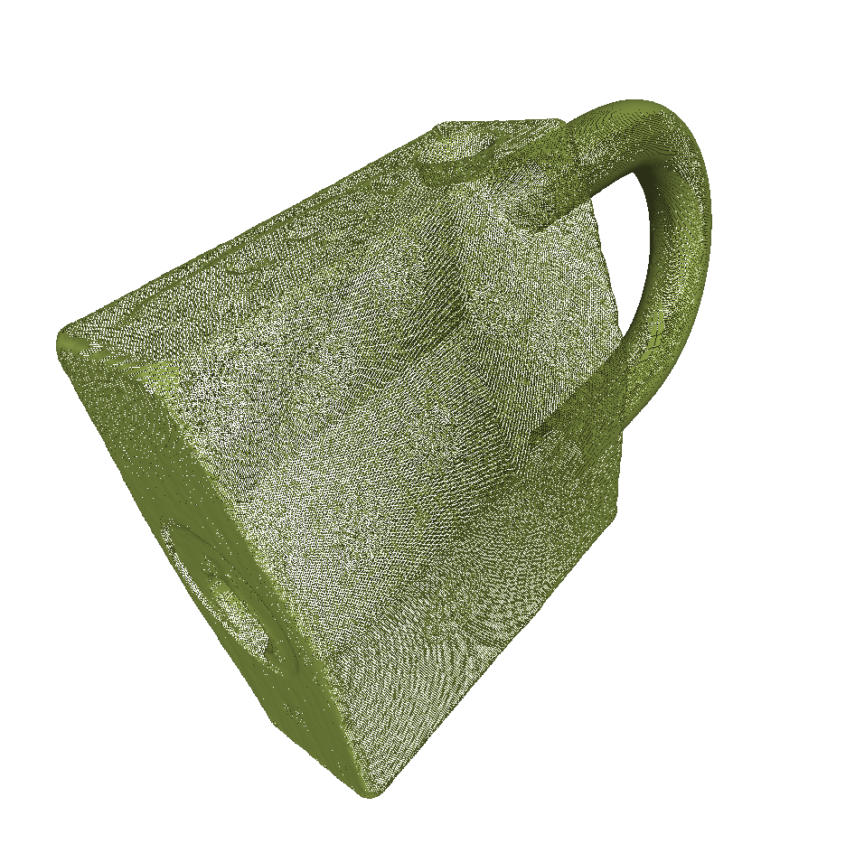
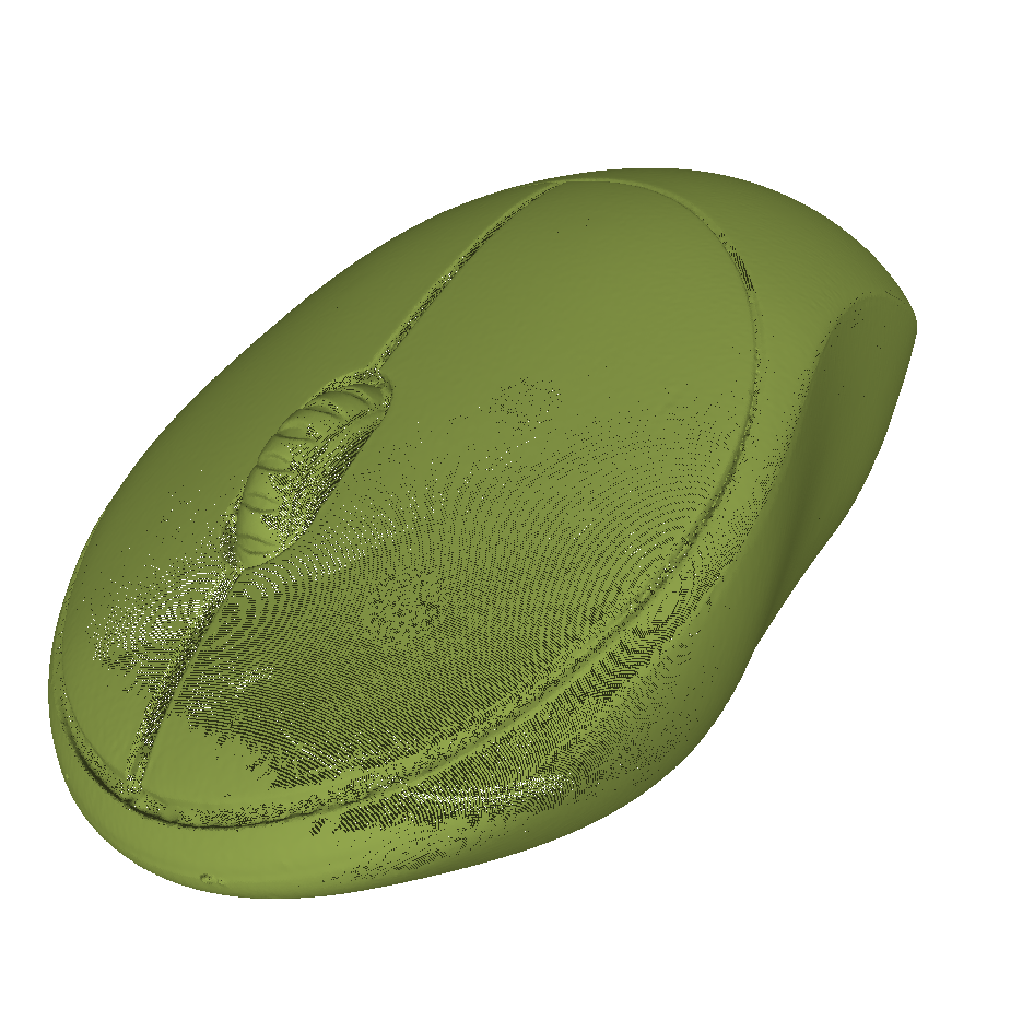
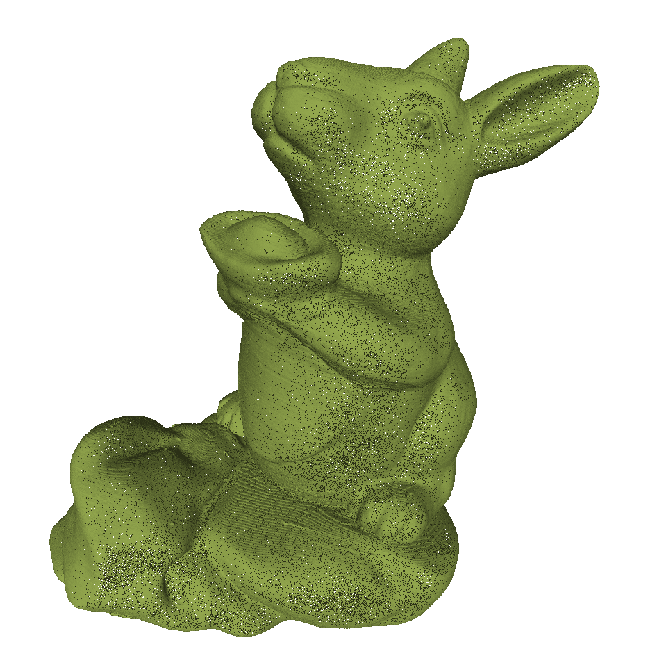
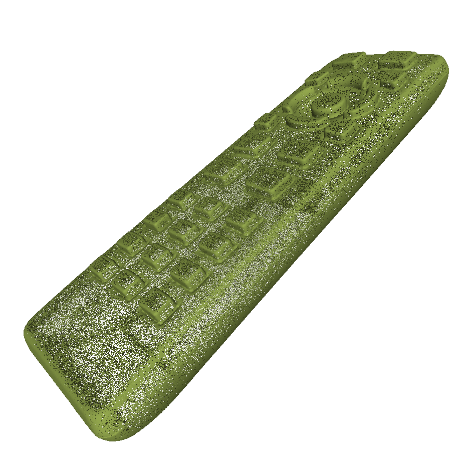
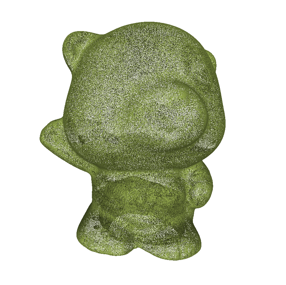
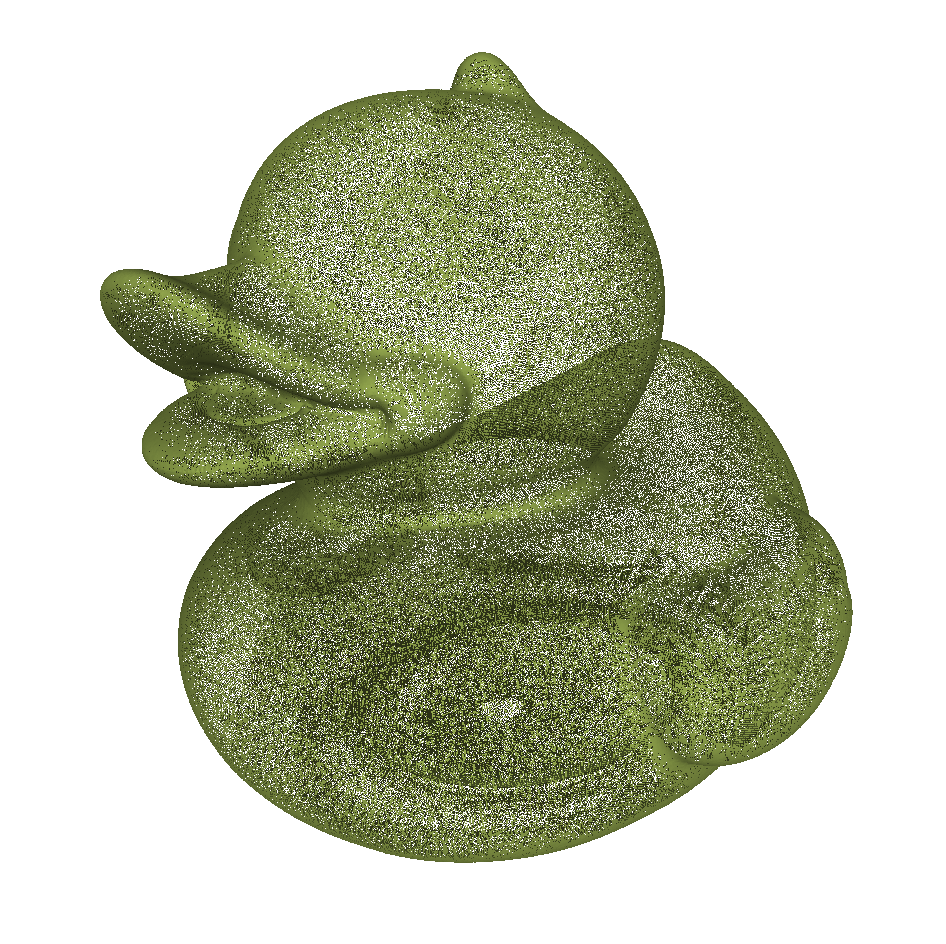
Figure 13: Real-world scanned models as point clouds as presented in [13]. From left to right: Bottle Shampoo, Bowl Chinese, Cloth Duck, Coffee Bottle Metal, Coffee Bottle Plastic, Cup, Flower Pot, Flower Pot 2, Gift Box, Lock, Mouse, Mug, Rabbit, Remote, Screw, Tape, Toy Bear, Toy Duck, Wrench, Xiao Jie Jie.

A.1 Window Size

As mentioned in the paper, the algorithm asks for a window size $w$, which is used to limit tracing along borders in order to place the next vertex candidate. Experiments run with different window sizes show that the triangulation quality and the number of triangles obtain plateau from $w=8$ onward. This makes $w=8$ a reasonable choice for a reliable output with respect to the occurring lengths of borders before triangulating the created regions. See the result of the experiments in Figures 14 and 15. All experiments were run on the Bottle Shampoo model.

On this model, the effect of changing the window sizes within this comparably small regime ([0,32]) is not measurable when considering the run time. That is on the one hand side because all these look-ups are constant-time as opposed to considering the entire border, which can grow towards an expected time of $\mathcal{O}(\sqrt{n})$ for $n$ vertices placed. On the other hand size, traversing a border for a small number of vertices already suffices to find that the traversed points are on the same border region. Thus, an increased window size does not have any effect on these specific queries.

Figure 14: Quality $Q(t)$ for varying window sizes.

Figure 15: Number of triangles for varying window sizes.

The window size $w$ influences the border length of the arising regions. As illustrated in Figure 3 in the article, a very small window size, i.e., $w=0$, results in borders up to length $93$ while increasing the window size to $w=8$ reduces the border length to $11$.

In contrast to the target edge length $d$ chosen to illustrate the effect on the Bottle Shampoo model in the paper, here, the target edge length is equal to $0.2$ to conincide with the other experiments presented in the supplementary material. As shown in Figure 16, a bigger window size $w$ prevents longer borders. Here, for $w=0$, the longest border is of length $80$ while for $w=8$, there is no region of border length bigger than $20$. Most resulting regions have a border length settled between $3$ and $12$ for both choices for $w$. Note that the histogram in Figure 16 has a log-scale $y$-axis. The obtained triangle quality stems to the largest extend from the placement of the vertices, rather than from triangulating regions with borders larger than $3$. Even though changing the window size does not influence the run time significantly, it influences the visual aspects of the output, but the mesh quality after trigangulating the regions remains untouched as aforementioned.

Figure 16: Region sizes for window sizes $w=0$ (shown in blue) and $w=8$ (shown in red) apllied to the Bottle Shampoo model.

A.2 Collection of Models

A.2.1 Bottle Shampoo Model

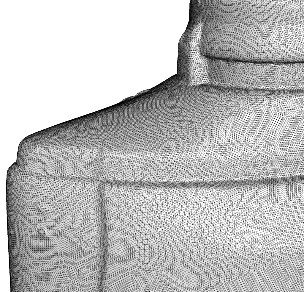
(a) Angle distribution, target=$60^{\circ}$.

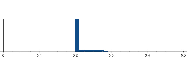
(b) Edge lengths distribution, target=0.2.

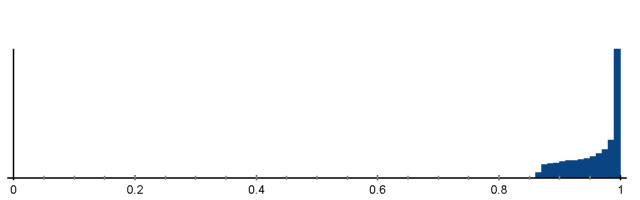
(c) Distribution of quality $Q(t)$, target=1.0.

Figure 17: Bottle Shampoo model.

Algorithm	$|\mathcal{T}|$	$E_{\text{avg}}$	$E_{\text{RMS}}$	$Q_{\text{avg}}$	$Q_{\text{RMS}}$
Adv. Front	1.209,546	0.1799	39.6	0.8247	16.0
Adv. Front (Re)	928,850	0.2028	15.3	0.9416	6.1
Poisson	16,280	1.2946	74.8	0.8760	12.3
Poisson (Re)	498,140	0.2657	38.6	0.9251	7.5
Poisson MG	150,770	0.5318	35.7	0.7204	33.7
Poisson MG (Re)	952,830	0.2015	16.3	0.9330	7.0
RIMLS	1,907,781	0.1499	35.8	0.7055	35.1
RIMLS (Re)	1,054,438	0.1905	19.3	0.9117	11.5
Scale Space	1,209,093	0.1798	39.1	0.8248	16.0
Scale Space (Re)	926,828	0.2028	15.2	0.9417	6.0
Voronoi	1,209,792	0.1799	52.3	0.8241	16.1
Voronoi (Re)	923,476	0.2044	20.8	0.9407	6.8
Ours	840,453	0.2131	11.2	0.9577	4.5
Ours (Re)	854,257	0.2098	10.4	0.9701	3.8

Table 5: Experimental results for the Bottle Shampoo model from [13] (604,903 points).

A.2.2 Bowl Chinese Model

(a) Angle distribution, target=$60^{\circ}$.

(b) Edge lengths distribution, target=0.2.

(c) Distribution of quality $Q(t)$, target=1.0.

Figure 18: Bowl Chinese model.

Algorithm	$|\mathcal{T}|$	$E_{\text{avg}}$	$E_{\text{RMS}}$	$Q_{\text{avg}}$	$Q_{\text{RMS}}$
Adv. Front	1,212,636	0.2920	38.2	0.8045	18.6
Adv. Front (Re)	2,407,002	0.2038	15.4	0.9405	6.2
Poisson	13,584	2.3850	63.2	0.8845	11.7
Poisson (Re)	637,488	0.3732	40.8	0.9301	6.9
Poisson MG	503,458	0.4710	39.8	0.7062	37.1
Poisson MG (Re)	2,409,076	0.2050	17.7	0.9223	7.9
RIMLS	6,458,589	0.1331	40.4	0.6877	39.6
RIMLS (Re)	2,441,143	0.2023	15.4	0.9394	6.3
Scale Space	1,093,339	0.2779	34.9	0.8054	18.7
Scale Space (Re)	1,947,592	0.2006	16.1	0.9351	7.3
Voronoi	1,212,636	0.2916	38.4	0.8042	18.7
Voronoi (Re)	2,398,584	0.2039	15.3	0.9405	6.1
Ours	2,137,650	0.2167	14.8	0.9485	6.2
Ours (Re)	2,246,434	0.2093	11.4	0.9665	4.3

Table 6: Experimental results for the Bowl Chinese model from [13] (606,320 points).

A.2.3 Cloth Duck Model

(a) Angle distribution, target=$60^{\circ}$.

(b) Edge lengths distribution, target=0.2.

(c) Distribution of quality $Q(t)$, target=1.0.

Figure 19: Cloth Duck model.

Algorithm	$|\mathcal{T}|$	$E_{\text{avg}}$	$E_{\text{RMS}}$	$Q_{\text{avg}}$	$Q_{\text{RMS}}$
Adv. Front	2,037,574	0.1839	40.1	0.8143	17.3
Adv. Front (Re)	1,739,214	0.1965	19.4	0.9179	9.5
Poisson	147,940	0.6300	44.3	0.8805	12.0
Poisson (Re)	1,488,112	0.2068	17.5	0.9311	7.2
Poisson MG	419,614	0.4086	38.5	0.7160	36.0
Poisson MG (Re)	1,463,018	0.2093	18.7	0.9154	8.8
RIMLS	5,878,521	0.1154	39.9	0.6919	38.9
RIMLS (Re)	1,728,371	0.1978	20.1	0.9143	12.7
Scale Space	2,036,816	0.1839	40.0	0.8139	17.4
Scale Space (Re)	1,735,814	0.1965	19.3	0.9179	9.5
Voronoi	2,037,270	0.1767	41.8	0.8067	18.1
Voronoi (Re)	1,514,160	0.2027	15.4	0.9407	6.3
Ours	1,435,604	0.2181	15.7	0.9454	6.6
Ours (Re)	1,535,058	0.2089	12.5	0.9592	4.8

Table 7: Experimental results for the Cloth Duck model from [13] (1,018,891 points).

A.2.4 Coffee Bottle Metal Model

(a) Angle distribution, target=$60^{\circ}$.

(b) Edge lengths distribution, target=0.2.

(c) Distribution of quality $Q(t)$, target=1.0.

Figure 20: Coffee Bottle Metal model.

Algorithm	$|\mathcal{T}|$	$E_{\text{avg}}$	$E_{\text{RMS}}$	$Q_{\text{avg}}$	$Q_{\text{RMS}}$
Adv. Front	1,211,290	0.2204	44.2	0.8036	18.4
Adv. Front (Re)	1,423,429	0.2029	15.2	0.9416	6.1
Poisson	25,842	1.2170	84.0	0.8743	12.4
Poisson (Re)	670,954	0.2805	41.6	0.9254	7.5
Poisson MG	249,103	0.5440	46.4	0.7265	33.0
Poisson MG (Re)	1,657,210	0.2097	20.8	0.9143	8.0
RIMLS	3,024,537	0.1477	35.4	0.7107	34.4
RIMLS (Re)	1,489,387	0.1986	18.0	0.9229	10.1
Scale Space	1,197,246	0.2188	43.4	0.8039	18.5
Scale Space (Re)	1,379,802	0.2021	15.5	0.9397	6.5
Voronoi	1,211,618	0.2198	52.6	0.8021	18.6
Voronoi (Re)	1,412,630	0.2043	21.1	0.9411	6.6
Ours	1,260,935	0.2162	14.0	0.9494	5.9
Ours (Re)	1,317,181	0.2095	11.4	0.9661	4.3

Table 8: Experimental results for the Coffee Bottle Metal model from [13] (605,826 points).

A.2.5 Coffee Bottle Plastic Model

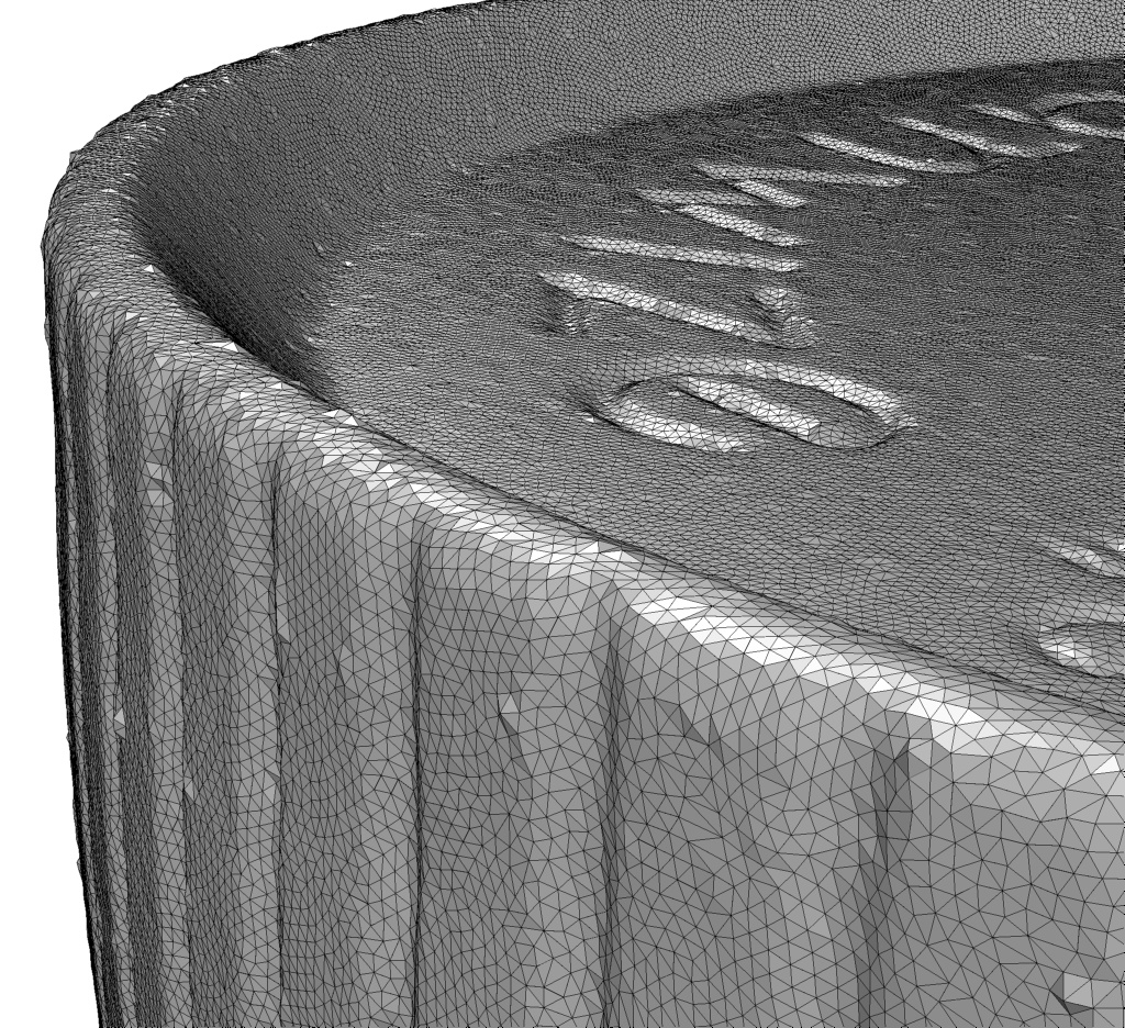
(a) Angle distribution, target=$60^{\circ}$.

(b) Edge lengths distribution, target=0.2.

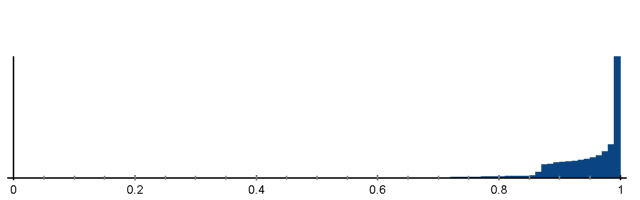
(c) Distribution of quality $Q(t)$, target=1.0.

Figure 21: Coffee Bottle Plastic model.

Algorithm	$|\mathcal{T}|$	$E_{\text{avg}}$	$E_{\text{RMS}}$	$Q_{\text{avg}}$	$Q_{\text{RMS}}$
Adv. Front	1,218,482	0.2128	45.7	0.8049	18.2
Adv. Front (Re)	1,359,038	0.2027	15.2	0.9417	6.1
Poisson	29,206	1.1586	76.5	0.8636	13.2
Poisson (Re)	746,200	0.2557	44.2	0.9205	7.8
Poisson MG	576,442	0.3273	35.4	0.7267	33.2
Poisson MG (Re)	1,530,906	0.1931	16.1	0.9134	5.8
RIMLS	7,438,789	0.0922	35.9	0.7121	34.8
RIMLS (Re)	1,308,171	0.2070	15.5	0.9373	6.5
Scale Space	1,204,794	0.2112	45.0	0.8050	18.2
Scale Space (Re)	1,316,070	0.2019	15.5	0.9398	6.4
Voronoi	1,218,482	0.2114	46.4	0.8028	18.4
Voronoi (Re)	1,341,154	0.2032	15.1	0.9422	6.0
Ours	1,203,156	0.2162	14.0	0.9495	5.8
Ours (Re)	1,257,141	0.2094	11.4	0.9659	4.3

Table 9: Experimental results for the Coffee Bottle Plastic model from [13] (609,243 points).

A.2.6 Cup Mpdel

(a) Angle distribution, target=$60^{\circ}$.

(b) Edge lengths distribution, target=0.2.

(c) Distribution of quality $Q(t)$, target=1.0.

Figure 22: Cup model.

Algorithm	$|\mathcal{T}|$	$E_{\text{avg}}$	$E_{\text{RMS}}$	$Q_{\text{avg}}$	$Q_{\text{RMS}}$
Adv. Front	2,820,618	0.1038	21.5	0.8978	6.1
Adv. Front (Re)	711,716	0.2032	15.0	0.9430	5.9
Poisson	31,450	0.8540	63.3	0.8744	12.5
Poisson (Re)	660,134	0.2110	19.5	0.9297	7.2
Poisson MG	605,996	0.2330	39.6	0.7050	37.2
Poisson MG (Re)	692,170	0.2064	17.1	0.9323	7.0
RIMLS	7,815,640	0.0658	40.2	0.6880	39.4
RIMLS (Re)	713,396	0.2040	16.5	0.9295	7.1
Scale Space	2,820,618	0.1038	21.5	0.8978	6.1
Scale Space (Re)	712,010	0.2031	15.0	0.9430	5.9
Voronoi	2,820,618	0.1035	21.6	0.8976	6.2
Voronoi (Re)	664,994	0.2097	14.8	0.9420	6.1
Ours	645,670	0.2133	11.3	0.9570	4.5
Ours (Re)	657,232	0.2099	10.6	0.9694	3.9

Table 10: Experimental results for the Cup model from [13] (1,410,309 points).

A.2.7 Flower Pot Model

(a) Angle distribution, target=$60^{\circ}$.

(b) Edge lengths distribution, target=0.2.

(c) Distribution of quality $Q(t)$, target=1.0.

Figure 23: Flower Pot model.

Algorithm	$|\mathcal{T}|$	$E_{\text{avg}}$	$E_{\text{RMS}}$	$Q_{\text{avg}}$	$Q_{\text{RMS}}$
Adv. Front	1,226,042	0.2780	46.1	0.8010	19.0
Adv. Front (Re)	2,304,698	0.2043	15.7	0.9376	6.5
Poisson	30,656	1.5601	67.1	0.8589	13.6
Poisson (Re)	1,164,952	0.2722	41.4	0.9157	8.1
Poisson MG	747,300	0.3767	36.6	0.7235	33.9
Poisson MG (Re)	2,296,376	0.2052	16.7	0.9247	8.2
RIMLS	9,625,452	0.1063	37.2	0.7050	36.1
RIMLS (Re)	2,252,713	0.2064	15.1	0.9410	6.2
Scale Space	1,057,169	0.2555	42.0	0.8017	19.1
Scale Space (Re)	1,644,152	0.1997	16.8	0.9288	8.3
Voronoi	1,226,042	0.2764	46.6	0.7996	19.2
Voronoi (Re)	2,284,266	0.2045	15.7	0.9378	6.4
Ours	2,052,950	0.2170	15.1	0.9476	6.4
Ours (Re)	2,161,017	0.2095	11.7	0.9642	4.6

Table 11: Experimental results for the Flower Pot model from [13] (613,021 points).

A.2.8 Flower Pot 2 Model

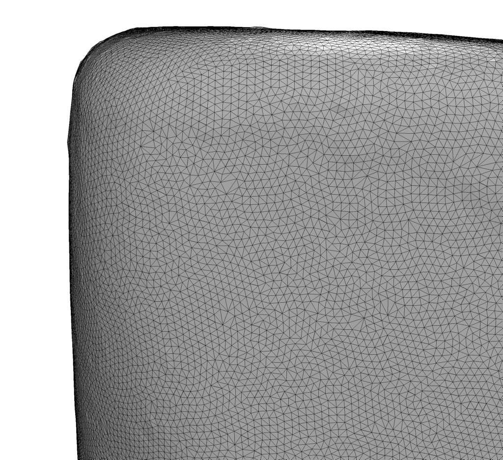
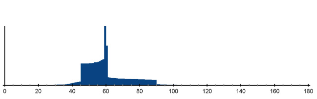
(a) Angle distribution, target=$60^{\circ}$.

(b) Edge lengths distribution, target=0.2.

(c) Distribution of quality $Q(t)$, target=1.0.

Figure 24: Flower Pot 2 model.

Algorithm	$|\mathcal{T}|$	$E_{\text{avg}}$	$E_{\text{RMS}}$	$Q_{\text{avg}}$	$Q_{\text{RMS}}$
Adv. Front	2,826,864	0.2135	38.1	0.8136	17.3
Adv. Front (Re)	3,001,322	0.2031	15.1	0.9425	5.9
Poisson	26,436	1.7814	80.3	0.8668	13.0
Poisson (Re)	1,062,612	0.3053	56.0	0.9198	7.7
Poisson MG	640,912	0.4605	36.4	0.7400	32.7
Poisson MG (Re)	3,016,388	0.2043	18.7	0.9180	8.4
RIMLS	8,225,140	0.1302	37.0	0.7205	35.3
RIMLS (Re)	2,939,770	0.2053	15.4	0.9392	6.7
Scale Space	2,815,621	0.2130	37.8	0.8138	17.2
Scale Space (Re)	2,969,237	0.2028	15.2	0.9418	6.1
Voronoi	2,826,862	0.2133	38.2	0.8133	17.3
Voronoi (Re)	2,985,334	0.2034	15.0	0.9428	5.9
Ours	2,661,776	0.2162	14.0	0.9494	5.9
Ours (Re)	2,782,563	0.2094	11.4	0.9662	4.3

Table 12: Experimental results for the Flower Pot 2 model from [13] (1,413,342 points).

A.2.9 Gift Box Model

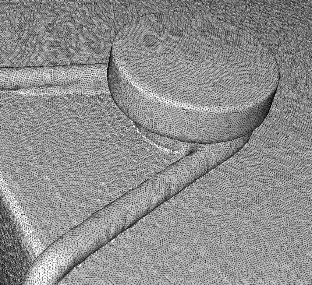
(a) Angle distribution, target=$60^{\circ}$.

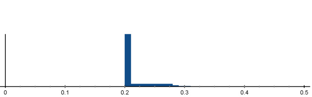
(b) Edge lengths distribution, target=0.2.

(c) Distribution of quality $Q(t)$, target=1.0.

Figure 25: Gift Box model.

Algorithm	$|\mathcal{T}|$	$E_{\text{avg}}$	$E_{\text{RMS}}$	$Q_{\text{avg}}$	$Q_{\text{RMS}}$
Adv. Front	3,063,655	0.1809	40.0	0.8313	15.7
Adv. Front (Re)	2,400,932	0.2022	15.5	0.9409	6.3
Poisson	68,578	0.7763	130.2	0.8681	12.9
Poisson (Re)	845,348	0.2990	62.8	0.9242	7.7
Poisson MG	400,500	0.6026	61.4	0.7877	24.7
Poisson MG (Re)	3,389,028	0.2185	31.1	0.9126	8.5
RIMLS	4,649,233	0.1531	74.9	0.7641	28.0
RIMLS (Re)	4,648,407	0.1522	75.2	0.7761	25.7
Scale Space	3,059,551	0.1808	39.9	0.8313	15.7
Scale Space (Re)	2,395,066	0.2020	15.6	0.9405	6.4
Voronoi	3,063,361	0.1796	40.7	0.8297	15.9
Voronoi (Re)	2,360,337	0.2028	15.3	0.9415	6.3
Ours	2,115,895	0.2164	14.2	0.9487	6.1
Ours (Re)	2,211,935	0.2096	11.8	0.9639	4.5

Table 13: Experimental results for the Gift Box model from [13] (1,532,008 points).

A.2.10 Lock Model

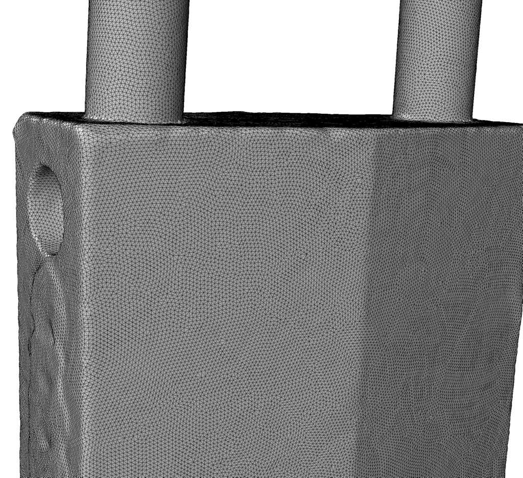
(a) Angle distribution, target=$60^{\circ}$.

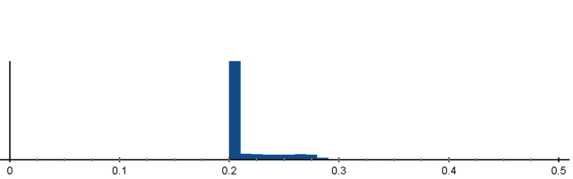
(b) Edge lengths distribution, target=0.2.

(c) Distribution of quality $Q(t)$, target=1.0.

Figure 26: Lock model.

Algorithm	$|\mathcal{T}|$	$E_{\text{avg}}$	$E_{\text{RMS}}$	$Q_{\text{avg}}$	$Q_{\text{RMS}}$
Adv. Front	668,388	0.1152	18.3	0.9227	6.6
Adv. Front (Re)	211,646	0.2035	15.0	0.9434	5.9
Poisson	12,598	0.6966	79.2	0.8654	13.1
Poisson (Re)	153,344	0.2318	33.9	0.9241	7.7
Poisson MG	201,226	0.2201	36.3	0.7118	34.4
Poisson MG (Re)	204,718	0.2078	17.0	0.9319	6.9
RIMLS	2,585,492	0.0620	36.7	0.6966	36.1
RIMLS (Re)	212,924	0.2043	16.9	0.9251	7.4
Scale Space	668,388	0.1152	18.3	0.9227	6.6
Scale Space (Re)	211,572	0.2036	15.0	0.9434	5.8
Voronoi	668,388	0.1147	18.5	0.9224	6.7
Voronoi (Re)	201,296	0.2089	15.5	0.9313	7.4
Ours	192,260	0.2136	11.6	0.9560	4.6
Ours (Re)	196,018	0.2101	11.0	0.9673	4.3

Table 14: Experimental results for the Lock model from [13] (334,194 points).

A.2.11 Mouse Model

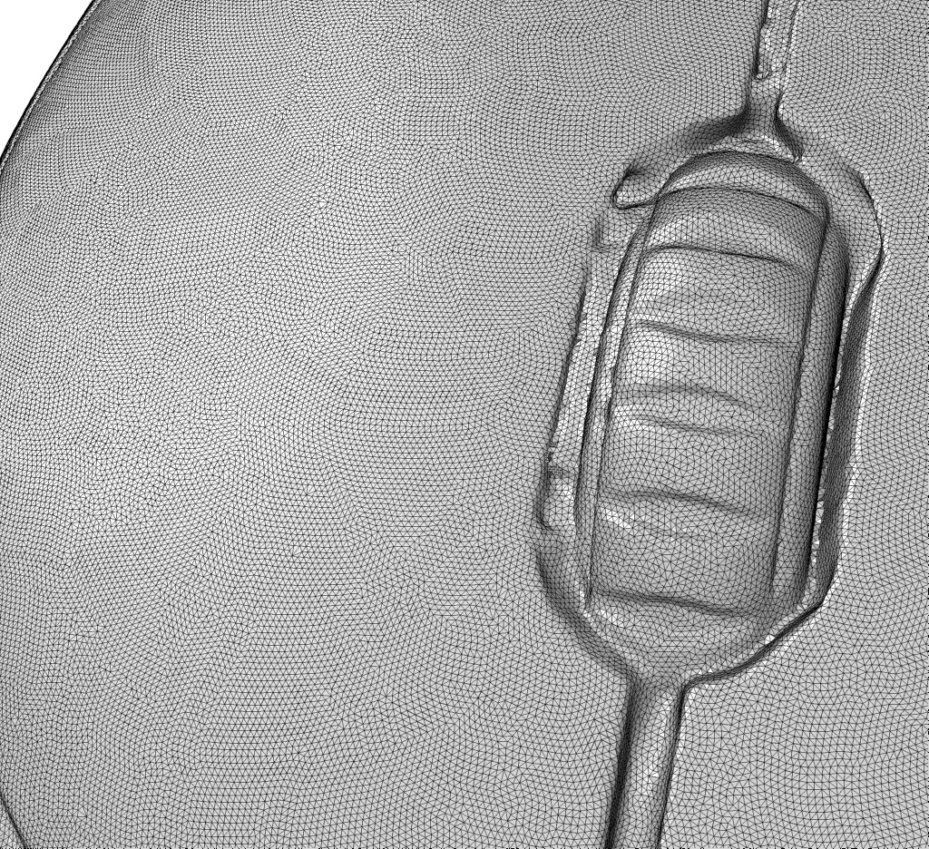
(a) Angle distribution, target=$60^{\circ}$.

(b) Edge lengths distribution, target=0.2.

(c) Distribution of quality $Q(t)$, target=1.0.

Figure 27: Mouse model.

Algorithm	$|\mathcal{T}|$	$E_{\text{avg}}$	$E_{\text{RMS}}$	$Q_{\text{avg}}$	$Q_{\text{RMS}}$
Adv. Front	2,564,191	0.1265	26.6	0.8806	8.2
Adv. Front (Re)	947,782	0.2036	15.2	0.9421	6.2
Poisson	33,934	0.8160	97.7	0.8711	12.9
Poisson (Re)	585,622	0.2521	34.8	0.9298	7.3
Poisson MG	265,630	0.4047	38.4	0.7125	35.7
Poisson MG (Re)	894,136	0.2108	18.2	0.9190	8.5
RIMLS	3,409,562	0.1145	39.1	0.6910	37.9
RIMLS (Re)	979,361	0.1984	22.2	0.9083	17.9
Scale Space	2,563,854	0.1265	26.6	0.8805	8.2
Scale Space (Re)	948,202	0.2035	15.2	0.9420	6.3
Voronoi	2,564,340	0.1262	26.9	0.8801	8.3
Voronoi (Re)	881,846	0.2103	14.2	0.9464	6.2
Ours	862,392	0.2134	11.5	0.9562	4.7
Ours (Re)	878,134	0.2100	10.9	0.9676	4.3

Table 15: Experimental results for the Mouse model from [13] (1,282,234 points).

A.2.12 Mug Model

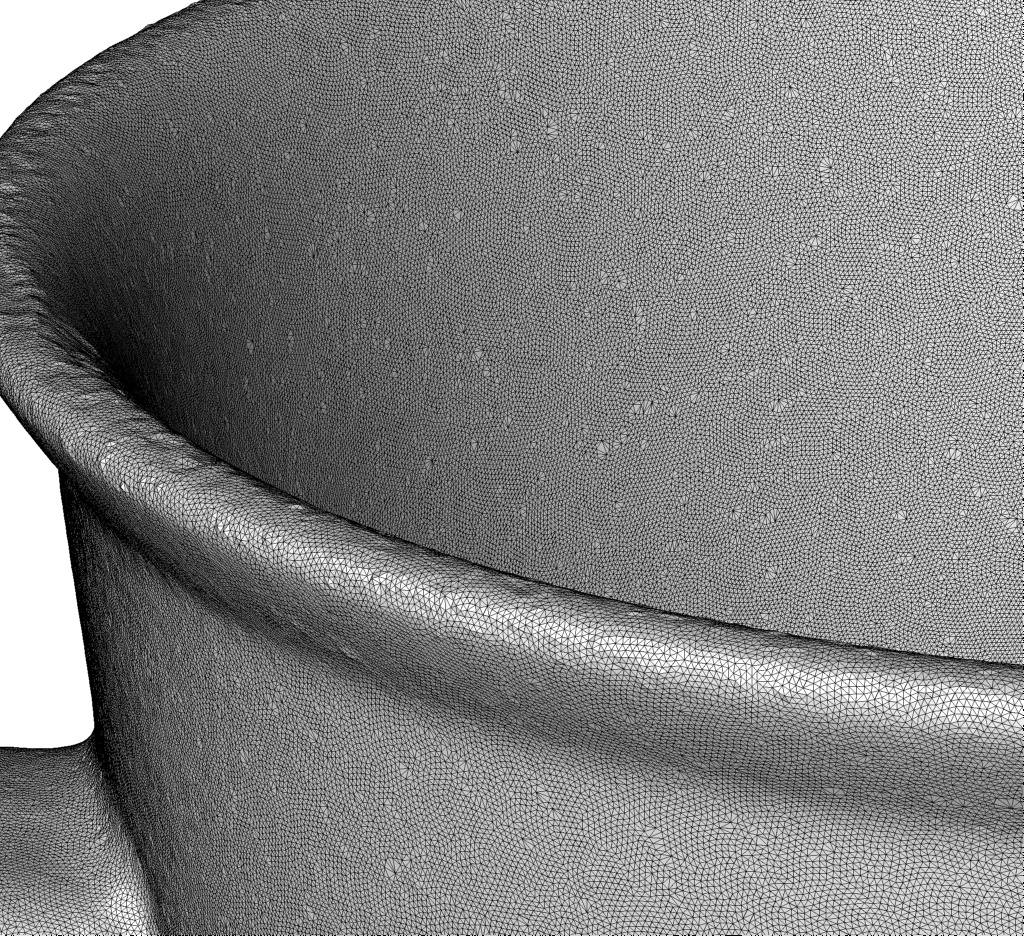
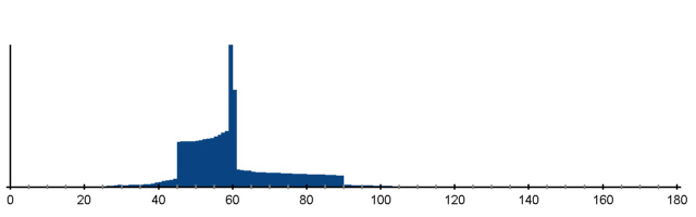
(a) Angle distribution, target=$60^{\circ}$.

(b) Edge lengths distribution, target=0.2.

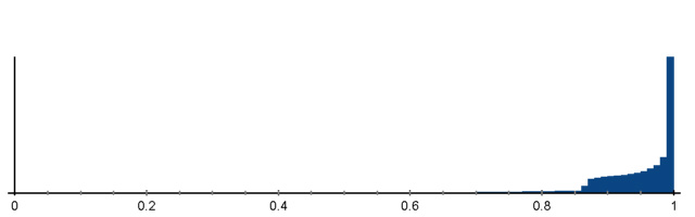
(c) Distribution of quality $Q(t)$, target=1.0.

Figure 28: Mug model.

Algorithm	$|\mathcal{T}|$	$E_{\text{avg}}$	$E_{\text{RMS}}$	$Q_{\text{avg}}$	$Q_{\text{RMS}}$
Adv. Front	1,212,626	0.3419	43.8	0.7999	19.1
Adv. Front (Re)	3,387,245	0.2049	15.9	0.9362	6.5
Poisson	16,520	2.5528	65.7	0.8822	11.8
Poisson (Re)	811,746	0.3845	47.9	0.9259	7.3
Poisson MG	550,330	0.5340	35.8	0.7233	33.3
Poisson MG (Re)	3,500,438	0.2016	16.1	0.9340	6.8
RIMLS	7,059,114	0.1507	36.3	0.7062	35.3
RIMLS (Re)	3,901,787	0.1919	16.8	0.9230	6.1
Scale Space	840,041	0.2861	36.8	0.8014	19.4
Scale Space (Re)	1,606,753	0.1985	17.3	0.9240	8.9
Voronoi	1,212,628	0.3413	44.0	0.7995	19.2
Voronoi (Re)	3,376,934	0.2050	15.9	0.9362	6.5
Ours	3,011,551	0.2175	16.2	0.9470	6.7
Ours (Re)	3,190,711	0.2093	11.7	0.9646	4.6

Table 16: Experimental results for the Mug model from [13] (606,322 points).

A.2.13 Rabbit Model

(a) Angle distribution, target=$60^{\circ}$.

(b) Edge lengths distribution, target=0.2.

(c) Distribution of quality $Q(t)$, target=1.0.

Figure 29: Rabbit model.

Algorithm	$|\mathcal{T}|$	$E_{\text{avg}}$	$E_{\text{RMS}}$	$Q_{\text{avg}}$	$Q_{\text{RMS}}$
Adv. Front	4,046,178	0.1563	45.4	0.7782	19.9
Adv. Front (Re)	2,370,715	0.2006	16.5	0.9337	7.2
Poisson	79,654	0.9804	60.4	0.8767	12.5
Poisson (Re)	1,851,254	0.2215	29.1	0.9264	7.5
Poisson MG	293,676	0.5974	38.4	0.7154	35.8
Poisson MG (Re)	2,559,026	0.1931	16.6	0.9216	6.1
RIMLS	3,573,629	0.1692	38.8	0.6973	38.1
RIMLS (Re)	2,631,908	0.1868	27.0	0.8500	22.9
Scale Space	4,041,938	0.1561	45.1	0.7782	19.9
Scale Space (Re)	2,357,012	0.2005	16.6	0.9332	7.3
Voronoi	4,046,157	0.1552	45.6	0.7767	20.0
Voronoi (Re)	2,323,985	0.2014	15.9	0.9374	6.5
Ours	2,039,974	0.2173	15.1	0.9470	6.4
Ours (Re)	2,152,626	0.2093	11.8	0.9636	4.5

Table 17: Experimental results for the Rabbit model from [13] (2,023,131 points).

A.2.14 Remote Model

(a) Angle distribution, target=$60^{\circ}$.

(b) Edge lengths distribution, target=0.2.

(c) Distribution of quality $Q(t)$, target=1.0.

Figure 30: Romoter model.

Algorithm	$|\mathcal{T}|$	$E_{\text{avg}}$	$E_{\text{RMS}}$	$Q_{\text{avg}}$	$Q_{\text{RMS}}$
Adv. Front	1,211,452	0.1681	40.7	0.8298	15.9
Adv. Front (Re)	826,007	0.2023	15.5	0.9405	6.3
Poisson	37,808	0.7858	78.8	0.8603	13.5
Poisson (Re)	603,656	0.2306	31.2	0.9232	7.7
Poisson MG	132,682	0.5261	37.1	0.7352	34.0
Poisson MG (Re)	829,026	0.2014	16.5	0.9318	7.3
RIMLS	1,691,586	0.1490	37.4	0.7162	36.6
RIMLS (Re)	1,006,124	0.1834	22.0	0.8900	15.7
Scale Space	1,211,373	0.1681	40.7	0.8298	15.9
Scale Space (Re)	825,804	0.2023	15.5	0.9404	6.3
Voronoi	1,211,428	0.1667	41.5	0.8275	16.1
Voronoi (Re)	806,808	0.2034	15.3	0.9415	6.2
Ours	726,550	0.2164	14.0	0.9488	5.9
Ours (Re)	760,465	0.2094	11.5	0.9654	4.4

Table 18: Experimental results for the Remote model from [13] (608,874 points).

A.2.15 Screw Model

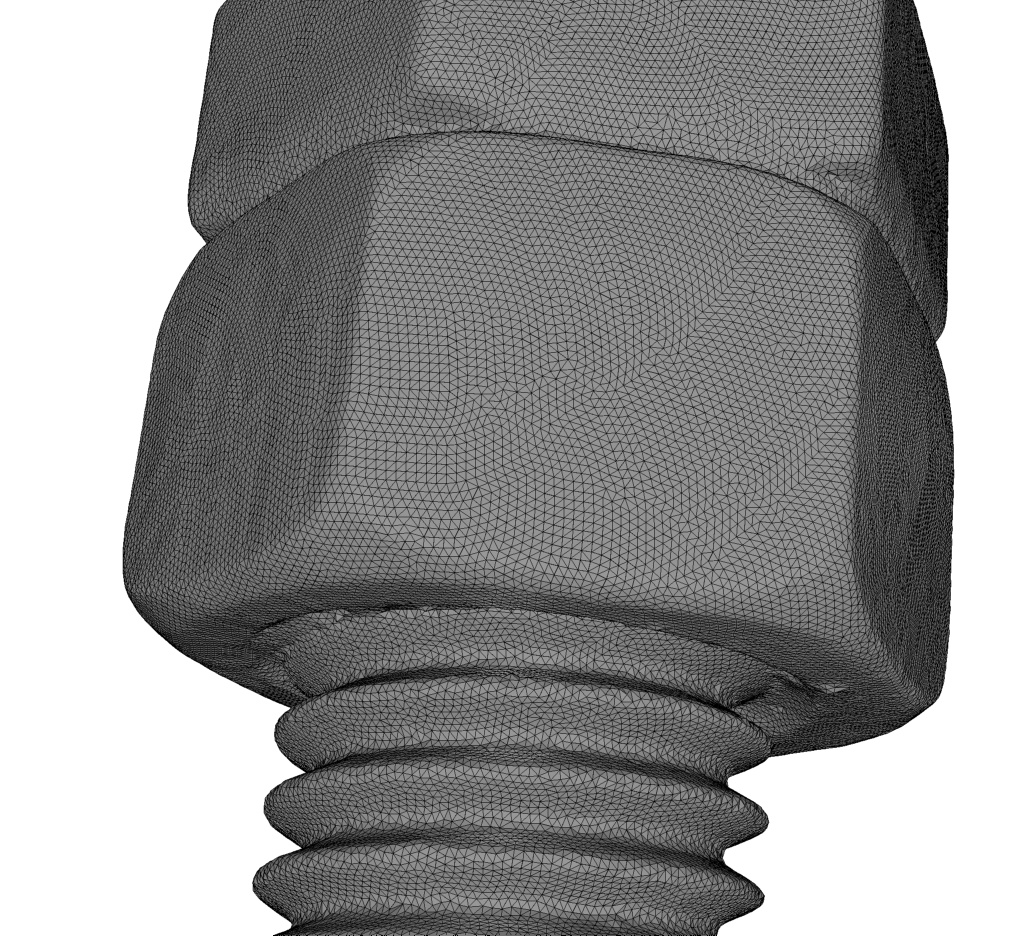
(a) Angle distribution, target=$60^{\circ}$.

(b) Edge lengths distribution, target=0.2.

(c) Distribution of quality $Q(t)$, target=1.0.

Figure 31: Screw model.

Algorithm	$|\mathcal{T}|$	$E_{\text{avg}}$	$E_{\text{RMS}}$	$Q_{\text{avg}}$	$Q_{\text{RMS}}$
Adv. Front	990,307	0.1102	23.3	0.8999	8.9
Adv. Front (Re)	283,248	0.2028	15.7	0.9397	6.5
Poisson	72,344	0.3693	56.8	0.8624	12.9
Poisson (Re)	268,408	0.2069	18.9	0.9271	7.5
Poisson MG	126,076	0.3162	39.7	0.7102	37.1
Poisson MG (Re)	297,510	0.1962	17.0	0.9176	8.6
RIMLS	1,687,736	0.0895	40.7	0.6873	40.0
RIMLS (Re)	284,956	0.2023	19.1	0.9228	12.4
Scale Space	990,296	0.1102	23.3	0.8999	8.9
Scale Space (Re)	283,400	0.2027	15.7	0.9397	6.6
Voronoi	990,314	0.1065	23.9	0.8970	9.3
Voronoi (Re)	252,708	0.2079	15.4	0.9394	6.6
Ours	254,936	0.2144	12.1	0.9531	5.0
Ours (Re)	261,268	0.2103	11.6	0.9633	4.4

Table 19: Experimental results for the Screw model from [13] (495,182 points).

A.2.16 Tape Model

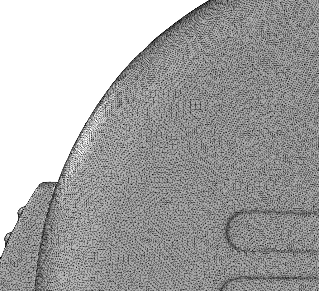
(a) Angle distribution, target=$60^{\circ}$.

(b) Edge lengths distribution, target=0.2.

(c) Distribution of quality $Q(t)$, target=1.0.

Figure 32: Tape model.

Algorithm	$|\mathcal{T}|$	$E_{\text{avg}}$	$E_{\text{RMS}}$	$Q_{\text{avg}}$	$Q_{\text{RMS}}$
Adv. Front	1,022,926	0.1693	47.8	0.8250	16.4
Adv. Front (Re)	704,575	0.2028	16.2	0.9385	7.1
Poisson	27,660	0.8333	83.3	0.8650	13.2
Poisson (Re)	474,692	0.2364	38.2	0.9203	7.9
Poisson MG	280,190	0.3369	35.6	0.7373	32.3
Poisson MG (Re)	773,900	0.1962	16.2	0.9097	6.1
RIMLS	3,577,797	0.0950	35.9	0.2486	34.5
RIMLS (Re)	680,432	0.2055	16.2	0.9357	7.6
Scale Space	1,021,944	0.1685	41.5	0.8255	16.2
Scale Space (Re)	698,119	0.2025	15.5	0.9405	6.3
Voronoi	1,023,090	0.1680	46.9	0.8234	16.5
Voronoi (Re)	690,444	0.2042	16.5	0.9400	6.8
Ours	616,091	0.2162	14.0	0.9491	5.8
Ours (Re)	643,856	0.2097	11.9	0.9633	4.7

Table 20: Experimental results for the Tape model from [13] (511,569 points).

A.2.17 Toy Bear Model

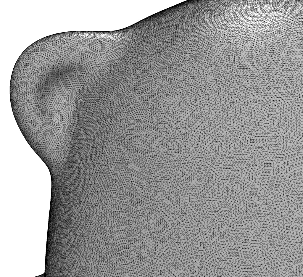
(a) Angle distribution, target=$60^{\circ}$.

(b) Edge lengths distribution, target=0.2.

(c) Distribution of quality $Q(t)$, target=1.0.

Figure 33: Toy Bear model.

Algorithm	$|\mathcal{T}|$	$E_{\text{avg}}$	$E_{\text{RMS}}$	$Q_{\text{avg}}$	$Q_{\text{RMS}}$
Adv. Front	1,214,998	0.1474	36.3	0.8474	13.9
Adv. Front (Re)	629,138	0.2024	15.2	0.9418	6.0
Poisson	20,134	1.0381	54.7	0.8882	11.7
Poisson (Re)	530,374	0.2193	22.8	0.9293	7.3
Poisson MG	432,268	0.2585	39.5	0.2623	37.1
Poisson MG (Re)	629,508	0.2021	15.0	0.9436	6.1
RIMLS	5,548,226	0.0730	40.0	0.6910	39.3
RIMLS (Re)	618,531	0.2049	16.2	0.9322	6.8
Scale Space	1,214,990	0.1474	36.3	0.8474	13.9
Scale Space (Re)	628,848	0.2025	15.2	0.9417	6.0
Voronoi	1,214,996	0.1471	36.5	0.8471	13.9
Voronoi (Re)	616,160	0.2041	15.0	0.9427	5.9
Ours	555,490	0.2159	13.5	0.9499	5.6
Ours (Re)	578,730	0.2096	11.5	0.9657	4.3

Table 21: Experimental results for the Toy Bear model from [13] (607,501 points).

A.2.18 Toy Duck Model

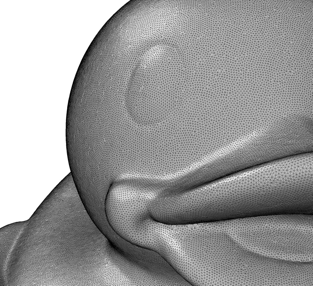
(a) Angle distribution, target=$60^{\circ}$.

(b) Edge lengths distribution, target=0.2.

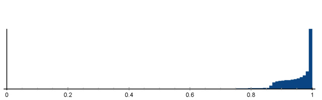
(c) Distribution of quality $Q(t)$, target=1.0.

Figure 34: Toy Duck model.

Algorithm	$|\mathcal{T}|$	$E_{\text{avg}}$	$E_{\text{RMS}}$	$Q_{\text{avg}}$	$Q_{\text{RMS}}$
Adv. Front	1,208,620	0.1523	36.7	0.8347	14.9
Adv. Front (Re)	664,788	0.2023	15.3	0.9412	6.1
Poisson	18,238	1.1320	51.1	0.8876	11.8
Poisson (Re)	578,760	0.2158	20.9	0.9337	7.0
Poisson MG	503,882	0.2456	39.4	0.7090	36.9
Poisson MG (Re)	642,274	0.2064	16.8	0.9315	6.8
RIMLS	6,470,657	0.0694	40.1	0.6910	39.4
RIMLS (Re)	655,847	0.2044	16.4	0.9310	7.0
Scale Space	1,208,618	0.1523	36.7	0.8347	14.9
Scale Space (Re)	664,854	0.2023	15.3	0.9412	6.1
Voronoi	1,208,620	0.1520	36.8	0.8345	14.9
Voronoi (Re)	654,288	0.2036	15.1	0.9422	6.0
Ours	585,744	0.2160	13.6	0.9497	5.7
Ours (Re)	610,908	0.2095	11.5	0.9658	4.3

Table 22: Experimental results for the Toy Duck model from [13] (604,312 points).

A.2.19 Wrench Model

(a) Angle distribution, target=$60^{\circ}$.

(b) Edge lengths distribution, target=0.2.

(c) Distribution of quality $Q(t)$, target=1.0.

Figure 35: Wrench model.

Algorithm	$|\mathcal{T}|$	$E_{\text{avg}}$	$E_{\text{RMS}}$	$Q_{\text{avg}}$	$Q_{\text{RMS}}$
Adv. Front	1,219,826	0.1335	33.7	0.8538	12.6
Adv. Front (Re)	516,056	0.2020	15.5	0.9401	6.2
Poisson	26,428	0.6729	99.7	0.8469	14.2
Poisson (Re)	300,868	0.2535	37.5	0.9190	7.9
Poisson MG	66,946	0.5781	31.9	0.7818	26.0
Poisson MG (Re)	496,824	0.2054	15.1	0.9358	6.8
RIMLS	801,420	0.1656	31.2	0.7667	28.2
RIMLS (Re)	638,096	0.1808	20.6	0.8739	13.4
Scale Space	1,219,826	0.1335	33.7	0.8538	12.6
Scale Space (Re)	516,184	0.2020	15.4	0.9403	6.2
Voronoi	1,219,826	0.1326	34.3	0.8543	12.7
Voronoi (Re)	503,056	0.2037	15.4	0.9402	6.2
Ours	454,492	0.2157	13.3	0.9508	5.5
Ours (Re)	472,946	0.2095	11.5	0.9655	4.4

Table 23: Experimental results for the Wrench model from [13] (609,911 points).

A.2.20 Xiao Jie Jie Model

(a) Angle distribution, target=$60^{\circ}$.

(b) Edge lengths distribution, target=0.2.

(c) Distribution of quality $Q(t)$, target=1.0.

Figure 36: Xiao Jie Jie model.

Algorithm	$|\mathcal{T}|$	$E_{\text{avg}}$	$E_{\text{RMS}}$	$Q_{\text{avg}}$	$Q_{\text{RMS}}$
Adv. Front	2,473,735	0.1198	27.2	0.8755	9.3
Adv. Front (Re)	811,986	0.2037	15.0	0.9433	6.0
Poisson	87,740	0.5677	55.9	0.8785	12.2
Poisson (Re)	755,538	0.2097	21.0	0.9321	7.1
Poisson MG	200,446	0.4316	39.7	0.7043	37.7
Poisson MG (Re)	786,370	0.2073	18.7	0.9152	8.7
RIMLS	2,528,244	0.1219	40.2	0.6833	40.0
RIMLS (Re)	1,066,017	0.1703	37.3	0.7956	34.3
Scale Space	2,473,712	0.1198	27.2	0.8750	9.3
Scale Space (Re)	812,416	0.2037	15.0	0.9432	6.0
Voronoi	2,473,692	0.1186	27.5	0.8751	9.4
Voronoi (Re)	753,938	0.2094	14.4	0.9463	5.8
Ours	739,325	0.2138	11.6	0.9557	4.6
Ours (Re)	754,086	0.2101	11.2	0.9663	4.4

Table 24: Experimental results for the Xiao Jie Jie model from [13] (1,236,884 points).

References

- [1] N. Amenta, S. Choi, and R. K. Kolluri. The power crust. In Proceedings of the Sixth ACM Symposium on Solid Modeling and Applications, SMA ’01, pages 249––266, New York, NY, USA, 2001. Association for Computing Machinery.
- [2] F. Bernardini, J. Mittleman, H. Rushmeier, C. Silva, and G. Taubin. The ball-pivoting algorithm for surface reconstruction. IEEE Transactions on Visualization and Computer Graphics, 5(4):349–359, 1999.
- [3] J.-D. Boissonnat, A. Lieutier, and M. Wintraecken. The reach, metric distortion, geodesic convexity and the variation of tangent spaces. Journal of Applied and Computational Topology, 3:29–58, 2019.
- [4] D. Boltcheva and B. Lévy. Surface reconstruction by computing restricted voronoi cells in parallel. Computer-Aided Design, 90:123–134, 2017.
- [5] R. Chaudhari, P. K. Loharkar, and A. Ingle. Medical applications of rapid prototyping technology. In Recent Advances in Industrial Production, pages 241–250. Springer, 2022.
- [6] P. Cignoni, M. Callieri, M. Corsini, M. Dellepiane, F. Ganovelli, and G. Ranzuglia. MeshLab: an Open-Source Mesh Processing Tool. In V. Scarano, R. D. Chiara, and U. Erra, editors, Eurographics Italian Chapter Conference, pages 129–136. The Eurographics Association, 2008.
- [7] D. Cohen-Steiner and F. Da. A greedy delaunay-based surface reconstruction algorithm. The Visual Computer, 20:4–16, 2004.
- [8] J. Digne, J.-M. Morel, C.-M. Souzani, and C. Lartigue. Scale space meshing of raw data point sets. Computer Graphics Forum, 30(6):1630–1642, 2011.
- [9] H. Edelsbrunner, D. Kirkpatrick, and R. Seidel. On the shape of a set of points in the plane. IEEE Transactions on Information Theory, 29(4):551–559, 1983.
- [10] S. Giraudot. Surface reconstruction from point clouds. In CGAL User and Reference Manual, page 5.5.1. CGAL Editorial Board, 2022.
- [11] R. H. Helle and H. G. Lemu. A case study on use of 3d scanning for reverse engineering and quality control. Materials Today: Proceedings, 45:5255–5262, 2021.
- [12] H. Huang, S. Wu, D. Cohen-Or, M. Gong, H. Zhang, G. Li, and B. Chen. L1-medial skeleton of point cloud. ACM Trans. Graph., 32(4):65–1, 2013.
- [13] Z. Huang, Y. Wen, Z. Wang, J. Ren, and K. Jia. Surface reconstruction from point clouds: A survey and a benchmark. arXiv preprint arXiv:2205.02413, 2022.
- [14] M. Kazhdan, M. Bolitho, and H. Hoppe. Poisson Surface Reconstruction. In A. Sheffer and K. Polthier, editors, Symposium on Geometry Processing, pages 61–70. The Eurographics Association, 2006.
- [15] M. Kazhdan and H. Hoppe. An adaptive multi-grid solver for applications in computer graphics. Computer Graphics Forum, 38(1):138–150, 2019.
- [16] D. Levin. The approximation power of moving least-squares. Mathematics of computation, 67(224):1517–1531, 1998.
- [17] B. Levy. Geogram. https://github.com/BrunoLevy/geogram, 2023.
- [18] H. Lipschütz, M. Skrodzki, U. Reitebuch, and K. Polthier. Single-sized spheres on surfaces (S4). Computer Aided Geometric Design, 85:101971, 2021.
- [19] W. K. Liu, S. Li, and H. Park. Eighty years of the finite element method: Birth, evolution, and future, 2021.
- [20] M. Ma, X. Yu, N. Lei, H. Si, and X. Gu. Guaranteed quality isotropic surface remeshing based on uniformization. Procedia engineering, 203:297–309, 2017.
- [21] N. Mellado, Q. Marcadet, L. Espinasse, P. Mora, B. Dutailly, S. Tournon-Valiente, and X. Granier. 3D-ARD: A 3d-acquired research dataset, June 2020.
- [22] N. J. Mitra, A. T. Nguyen, and L. J. Guibas. Estimating surface normals in noisy point cloud data. In SCG ’03, pages 322–328, 2003.
- [23] C. Öztireli, G. Guennebaud, and M. Gross. Feature Preserving Point Set Surfaces based on Non-Linear Kernel Regression. Computer Graphics Forum, 28(2):493–501, 2009.
- [24] J. R. Shewchuk. What is a good linear element? Interpolation, conditioning, anisotropy, and quality measures. In 11th International Meshing Roundtable, pages 115–126, 2002.