Bayesian analysis of muon capture on deuteron in chiral effective field theory

Abstract

We compute the muon capture on deuteron in the doublet hyperfine state for a variety of nuclear interactions and consistent nuclear currents. Our analysis includes a detailed examination of the theoretical uncertainties coming from different sources: the single-nucleon axial form factor (providing $78.5\%$ of the total error), the truncation of the interaction and current chiral expansion (providing $0.8\%$ and $5.2\%$ of the total error, respectively), and the model dependence (providing $15.5\%$ of the total error). To estimate the truncation error of the chiral expansion of interactions and currents we use the most modern techniques based on Bayesian analysis. This method enables us to give a clear statistical interpretation of the computed theoretical uncertainties. Additionally, we provide the differential capture rate as function of the kinetic energy of the outgoing neutron which may be measured in future experiments. Our recommended theoretical value for the total capture rate is $\Gamma_{\rm th}=393.8\pm 4.4$ s^-1 ($68\%$ confidence level).

I Introduction

The muon capture on deuteron, i.e. the process

$$\mu^{-}+d\rightarrow n+n+\nu_{\mu}$$ (1)

is one of the electroweak processes that is accessible experimentally and at the same time can be computed using the most modern theoretical nuclear physics techniques combining chiral effective field theory ($\chi$EFT) with ab-initio numerical methods. This makes the reaction in Eq. (1) the ideal system for testing $\chi$EFT interactions and electroweak currents.

The experimental results for the total capture rate in the initial doublet hyperfine state $\Gamma$ Wang et al. (1965); Bertin et al. (1973); Bardin et al. (1986); Cargnelli M, et al. (1989) are relatively old and have large error-bars that make them compatible within each other but hard to use for precision tests of the theory. To improve the precision of experimental measurements, an on-going experiment at the Paul Scherrer Institute, in Switzerland, performed by the MuSun Collaboration, aims to reduce the uncertainty at the order of $\sim 1.5\%$ P. Kammel on behalf of the MuSun collaboration (2021). If such precision is achieved, it will enable more stringent test of the $\chi$EFT predictions.

On the theory side, several calculations have been carried out. A review of the theoretical results from up to about ten years ago can be found in Ref. Marcucci (2012). Some more recent calculations, but not yet fully within the $\chi$EFT framework, have been performed also in Refs. Marcucci et al. (2011); Golak et al. (2014). The first steps within the “hybrid” $\chi$EFT approach, where phenomenological potentials are used together with $\chi$EFT nuclear currents, have been performed in Refs. Marcucci et al. (2011); Ando et al. (2002). On the other hand, the first fully consistent $\chi$EFT calculations are those of Refs. Marcucci et al. (2012); Adam et al. (2012). To be remarked that the results of Ref. Marcucci et al. (2012), as well as those of Ref. Adam et al. (2012), were affected by a widely-spread error in the relation between the low-energy constant (LEC) entering the three-nucleon interaction and that one entering the axial current. In Ref. Marcucci et al. (2020) such error was spotted and the results of Ref. Marcucci et al. (2012) were corrected. In the last years, a fully consistent $\chi$EFT calculation, not affected by the above mentioned error, has been performed in Ref. Acharya et al. (2018). This work addressed also the impact of the experimental uncertainty on the single-nucleon axial form factor Hill et al. (2018). To be noticed that the work in Ref. Acharya et al. (2018) retained only the ${}^{1}S_{0}$ channel while in that of Bonilla et al. in Ref. Bonilla et al. (2023) a complete partial wave expansion was performed together with an analysis of the theoretical uncertainties to study the capture rate in both the $f=1/2$ and $f=3/2$ hyperfine states.

This work moves on a parallel line, starting from our recent paper where we considered only the ${}^{1}S_{0}$ neutron-neutron channel  Ceccarelli et al. (2023). We complete the calculation of Ref. Ceccarelli et al. (2023) adding the missing channels with a dual purpose. The first is to have the most robust theoretical error estimate based on the Bayesian analysis of the truncation errors of the chiral current and interaction expansions, on the model dependence, and on the propagation of the uncertainties related to the LECs appearing in the currents. For the Bayesian analysis we use the approach introduced in Ref. Melendez et al. (2019) and already employed in several works to give reliable estimates of truncation errors in chiral effective field theory (see Ref. buq for a complete list of works). The second is to compute the spectra of the outgoing neutrons as function of the kinetic energy of the neutron. Beyond the technical details, this kind of spectrum can possibly be measured in MuSun experiment Andreev et al. (2010) and can be useful for the simulation of the experimental apparatus, and consequently for data analysis.

The paper is organized as follow. In the next Section we will introduce the theoretical formalism giving the explicit expression for the differential capture rate as function of the kinetic energy of the neutron. In Section III we present the nuclear interaction and current models used in this work. Section IV is dedicated to a detailed examination of the theoretical uncertainties. In Section V, we discuss our results comparing them with the recent literature. Finally, in Section VI we consider the impact of our results on the analysis of the future data of the MuSun experiment.

II Muon capture on deuteron fundamentals

In the past literature the muon capture differential capture rate was computed versus the relative momenta of the two emitted neutrons. This has the advantage to reduce the numerical effort needed in the calculation. On the other hand, this is not what can be measured experimentally. In this work we consider the differential capture rate as function of the kinetic energy of one of the emitted neutrons (i.e. $E_{1}^{\prime}=E_{1}-m_{n}$), which is the quantity that can potentially be measured in an experiment using a neutron detector. Let us begin with the Fermi Golden Rule, that reads

$$d\Gamma=(2\pi)\delta(E_{1}+E_{2}+k_{\nu}-m_{\mu}-m_{d})\overline{|T_{fi}|^{2}}\frac{d{\bf p}_{1}}{(2\pi)^{3}}\frac{d{\bf k}_{\nu}}{(2\pi)^{3}}\,,$$ (2)

where $E_{1}(E_{2})$ is the energy of the first (second) outgoing neutron, $k_{\nu}$ the energy of the emitted neutrino, ${\bf p}_{1}({\bf p}_{2})$ the momenta of the first (second) outgoing neutron and ${\bf k}_{\nu}$ the momentum of the outgoing neutrino. Note that the phase space of the second emitted neutron has been eliminated using the conservation of the momenta. The transition amplitude is written as in Ref. Marcucci et al. (2011)

$$\overline{|T_{fi}|^{2}}=\frac{1}{2f+1}\sum_{s_{1}s_{2}h_{\nu}}\sum_{f_{z}}|T_{fi}(f,f_{z};s_{1},s_{2},h_{\nu})|^{2}\ ,$$ (3)

where $f,f_{z}$ indicate the initial hyperfine state (in this work we consider only $f=1/2$), while $s_{1}$, $s_{2}$, and $h_{\nu}$ denote the spin $z$-projection for the two neutrons and the neutrino helicity state. In turn, $T_{fi}(f,f_{z};s_{1},s_{2},h_{\nu})$ is given by

$$T_{fi}(f,f_{z};s_{1},s_{2},h_{\nu}) \equiv \langle nn,s_{1},s_{2};\nu,h_{\nu}\,|\,H_{W}\,|\,(\mu,d);f,f_{z}\rangle$$ (4)

$$\simeq {G_{V}^{\prime}\over\sqrt{2}}\psi_{1s}M_{fi}(f,f_{z};s_{1},s_{2},h_{\nu})\,,$$

where we have defined

$$M_{fi}(f,f_{z};s_{1},s_{2},h_{\nu}) =\sum_{s_{\mu}s_{d}}\langle{1\over 2}s_{\mu},1s_{d}|ff_{z}\rangle\,l_{\sigma}(h_{\nu},\,s_{\mu})$$ (5)

$$\times\langle\Psi_{{\bf p},s_{1}s_{2}}(nn)|j^{\sigma}({\bf q})|\Psi_{s_{d}}(d)\rangle\ .$$

with $l_{\sigma}$ and $j^{\sigma}$ being the leptonic and hadronic current densities respectively Marcucci et al. (2011). Here the leptonic momentum transfer ${\bf q}$ is defined as ${\bf q}\simeq-{\bf k}_{\nu}$ and ${\bf p}=({\bf p}_{1}-{\bf p}_{2})/2$ is the relative momentum among the two neutrons. Furthermore, $\Psi_{d}(s_{d})$ and $\Psi_{{\bf p},s_{1}s_{2}}(nn)$ are the deuteron and final $nn$ wave functions, respectively, with $s_{d}$ indicating the deuteron spin $z$-projection, which is computed using the variational method described in Refs. Marcucci et al. (2011); Ceccarelli et al. (2023). The final $nn$ wave function $\Psi_{{\bf p},s_{1}s_{2}}(nn)$ can be expanded in partial waves as

$$\Psi_{{\bf p},s_{1}s_{2}}(nn) = 4\pi\sum_{S}\langle\frac{1}{2}s_{1},\frac{1}{2}s_{2}|SS_{z}\rangle\sum_{LL_{z}JJ_{z}}{\rm i}^{L}Y^{*}_{LL_{z}}({\hat{\bf p}})$$ (6)

$$\times \langle SS_{z},LL_{z}|JJ_{z}\rangle\,\overline{\Psi}_{nn}^{LSJJ_{z}}(p)\>\>,$$

where $\overline{\Psi}_{nn}^{LSJJ_{z}}(p)$ is the $nn$ wave function with orbital angular momentum $LL_{z}$, total spin $SS_{z}$, and total angular momentum $JJ_{z}$ that is computed numerically by using the Kohn variational principle (see Ref. Kohn (1948)). The calculation is performed using partial waves up to $J=4$. The contribution to the total capture rate of the partial waves with $J>2$ is of the order of $0.75\%$. Finally, in Eq. (4), the function $\psi_{1s}$ is the average over the nuclear volume of the muon wave function in $1s$ orbit Marcucci et al. (2011); Walecka (1995), namely

$$|\psi_{1s}|\simeq|\psi_{1s}^{\rm av}|\equiv\,|\psi_{1s}(0)|\,=\,\sqrt{{(\alpha\,\mu_{\mu d})^{3}\over\pi}}\ ,$$ (7)

where $\psi_{1s}(0)$ denotes the Bohr wave function for a point charge $e$ evaluated at the origin, $\mu_{\mu d}$ is the reduced mass of the $(\mu,d)$ system, and $\alpha$ is the fine-structure constant. The integration of the matrix elements $M_{fi}$ is performed using Gaussian-Legendre quadrature with $\sim 50$ points on the angles and $\sim 70$ on the inter-nucleon distance $r$. This permits full convergence of the integrals.

Without losing generality we can choose ${\bf q}\parallel\hat{z}$ and define the angle $\theta_{1}$ as the angle between ${\bf q}$ and ${\bf p}_{1}$. After exploiting the conservation of energy in Eq. (2) the differential capture rate reads

$$\Gamma(E_{1}^{\prime}) = \frac{G_{V}^{{}^{\prime}2}}{\pi}|\psi_{1s}(0)|^{2}E_{1}p_{1}\int d\cos\theta_{1}\frac{E_{2}k_{\nu}^{2}}{E_{2}+k_{\nu}+p_{1}\cos\theta_{1}}$$ (8)

$$\times \sum_{s_{1}s_{2}h_{\nu}}\sum_{f_{z}}|M_{fi}(f_{z},s_{1},s_{2},h_{\nu};p_{1},\cos\theta_{1})|^{2}$$

where $k_{\nu}$ and $E_{2}$ can be easily obtained by the momentum and energy conservation. Note that in this case the scattering wave function depends explicitly on $p_{1}$ and $\cos\theta_{1}$ through ${\bf p}$ making the calculation much more expensive.

The total capture rate is then computed integrating directly on the kinetic energy $E_{1}^{\prime}$

$$\Gamma=\int_{0}^{E_{1}^{{}^{\prime}\rm max}}dE_{1}^{\prime}\,\Gamma(E_{1}^{\prime})\,.$$ (9)

The integrations on $E_{1}^{\prime}$ and $\cos\theta_{1}$ has been performed using Gauss-Legendre quadrature. To reach convergence we need to use at least 50 points on $E_{1}^{\prime}$ and 40 on $\cos\theta_{1}$. The total capture rate was also computed using the standard approach as in Ref. Marcucci et al. (2011), obtaining on the total capture rate numerical differences below 0.1 s^-1 for each nuclear interaction considered. In Table 1 we report the constants and the masses used in this work. Note that the vector coupling constant that first appears in Eq. (4) is

$$G_{V}^{{}^{\prime}2}=G_{V}^{2}(1+\Delta_{R}^{V})\,,$$ (10)

where the vector coupling constant $G_{V}$ is given by $G_{V}=1.1357\times 10^{-11}$ MeV^-2, and the process independent radiative correction $\Delta_{R}^{V}$ is $\Delta_{R}^{V}=0.02454$, according to the new updated values of Ref. Hardy and Towner (2020). The final value is then $G_{V}^{\prime}=1.149\times 10^{-11}$ MeV^-2.

$G_{V}^{\prime}$	$1.149\cdot 10^{-11}$ MeV-2
$1/\alpha$	$137.04$
$m_{d}$	$1875.61$ MeV
$m_{n}$	$939.57$ MeV
$m_{\mu}$	$105.66$ MeV

Table 1: Values of the constants used in the present calculation.

III Nuclear interactions and electroweak currents

The interactions we use in the present calculation are of two types. The first ones, developed in Norfolk (NV) Piarulli et al. (2015, 2016), are local interactions up to the next-to-next-to-next-to-leading-order (N3LO), and include $\Delta$-isobars together with pions and nucleons as degrees of freedom. The interactions are regularized in configuration-space with two regulators, one ($R_{S}$) for the short-range components associated with $2N$ contact terms, and the other ($R_{L}$) for the long-range terms. We consider four different interactions of this family for which two different sets of regulators have been used. The LECs have been fitted considering the $2N$ database within two different energy ranges.

The second family of interactions considered in this work is the one developed by Entem, Machleidt and Nosyk (EMN) in Ref. Entem et al. (2017). These interactions are implemented in momentum space and are strongly non-local. The degrees of freedom are pions and nucleons only. For this interaction family all the orders up to the next-to-next-to-next-to-next-to-leading-order (N4LO) are available for three different cutoff values $\Lambda\,$=$\,450$, $500$ and $550$ MeV. The LECs of these interactions are fixed fitting the $2N$ database up to $300$ MeV. In Table 2 we summarize the names of the interactions used in this work and their specific characteristics.

Name	DOF	$O_{\chi}$	$(R_{\rm S},R_{\rm L})$ or $\Lambda$	$E$ range	Space
NVIa	$\pi,N,\Delta$	N3LO	$(0.8,1.2)$ fm	0–125 MeV	$r$
NVIb	$\pi,N,\Delta$	N3LO	$(0.7,1.0)$ fm	0–125 MeV	$r$
NVIIa	$\pi,N,\Delta$	N3LO	$(0.8,1.2)$ fm	0–200 MeV	$r$
NVIIb	$\pi,N,\Delta$	N3LO	$(0.7,1.0)$ fm	0–200 MeV	$r$
EMN450	$\pi,N$	N4LO	$450$ MeV	0–300 MeV	$p$
EMN500	$\pi,N$	N4LO	$500$ MeV	0–300 MeV	$p$
EMN550	$\pi,N$	N4LO	$550$ MeV	0–300 MeV	$p$

Table 2: Summary of $2N$ interactions utilized in this study. In the first column we indicate the name adopted to identify each interaction and in the remaining columns we list its main features, including degrees of freedom (DOF), chiral order ($O_{\chi}$), cutoff values, lab-energy range over which the fits to the $2N$ database have been carried out ($E$ range), and whether it is expressed in configuration ($r$) or in momentum ($p$) space.

The adopted models for the nuclear axial and vector currents are the ones derived in Refs. Baroni et al. (2016, 2018) for the NV potentials and Refs. Pastore et al. (2009); Piarulli et al. (2013) for the EMN ones, respectively. Note that the vector weak operators are related to their electromagnetic counterpart via a rotation in the isospin space, and therefore in the following we will discuss the axial and the electromagnetic nuclear currents. In Table 3 we summarize the various contributions to the currents indicating the chiral orders at which they belong.

Oper.	LO $(Q^{-3})$	NLO $(Q^{-2})$	N2LO $(Q^{-1})$	N3LO $(Q^{0})$	N4LO $(Q^{1})$
$\rho(A)$	–	1b(NR)	OPE	–	TPEA
					CT†
${\bf j}(A)$	1b(NR)	–	1b(RC)	CT($z_{0}$)	TPE
			OPE-$\Delta^{*}$	OPE(sub)	OPE(sub)
$\rho(V)$	1b(NR)	–	1b(RC)	OPE	TPE
${\bf j}(V)$	–	1b(NR)	OPE	1b(RC)	TPE
				OPE-$\Delta^{*}$	OPE($d_{2}^{V}$, $d_{3}^{V}$, $d_{2}^{S}$)
					CT($d_{1}^{V}$, $d_{1}^{S}$)

Table 3: Ordering of the chiral electroweak currents as given in Refs. Baroni et al. (2016, 2018); Pastore et al. (2009); Piarulli et al. (2013). The acronym stands for 1b=one-body, OPE=one-pion exchange, CT=contact terms, TPE=two-pion exchange, NR=non-relativistic, RC=relativistic corrections, OPE-$\Delta$ = one-pion-exchange currents with an intermediate delta excitation, and sub=sub-leading. With the asterisk we indicate the terms that do not appear for the EMN interactions. The term with the superscript $A$ are not yet available for the NV interactions. The dagger indicates that the LECs appearing in these terms have not been determined yet. Note that we explicitly show for each term the LECs that have been fitted on electroweak processes.

Several LECs that appear in the nuclear currents are not fixed in the nuclear interactions. In the contact term (CT) of the axial current at N3LO is present the LEC $z_{0}$. Since this LEC is linearly dependent on the LEC $c_{D}$ that appear in the three-nucleon interaction, $z_{0}$ has been determined fitting contemporary the ³H binding energy and the Gamow-Teller matrix element of the ³H $\beta$-decay. The value of $c_{D}$ used in this work can be found in Ref. Baroni et al. (2018) and Ref. Marcucci et al. (2019) (Table II) for the NV and EMN interactions, respectively. At the same order the axial current presents also a subleading one-pion exchange (OPE) contribution. The other contributions at N3LO come from the OPE of the vector charge, the one-body relativistic corrections and the $\Delta$ OPE contribution at the level of the vector current present only for the NV potentials.

The situation regarding the currents at N4LO is more complex. The axial charge has a two-pion exchange (TPE) term, which is not yet available for the NV interactions, as well as two CTs whose constants have not been fitted. The axial current is generated by contributions coming from subleading OPE and TPE diagrams. On the other hand, the vector charge only receives contributions from TPE diagrams at this order. Finally, the vector current at N4LO is generated by TPE diagrams, as well as OPE and contact terms. Note that in the vector current, five independent LECs appear: $d_{2}^{V}$, $d_{3}^{V}$, $d_{2}^{S}$ associated with the OPE diagrams, and $d_{1}^{V}$ and $d_{1}^{S}$ associated with the CT diagrams. These are fixed in Ref. Gnech and Schiavilla (2022) for both the NV and EMN interactions on the magnetic moments of deuteron, ³H, and ³He and the electro-disintegration of deuteron at backward angles and can be found in Ref. Gnech and Schiavilla (2022) labeled as set A.

The calculation of the differential and total muon capture rate on deuteron presented below has been carried out for all the nuclear interactions presented in Table 2 and for all the chiral order from LO to N4LO in the case of the EMN interactions.

IV Analysis of the theoretical uncertainties

In this Section we are going to focus on the sources of uncertainties and on how we dealt with them. The sources of uncertainties that we consider are four: (i) the uncertainties on the LECs appearing in the nuclear electroweak currents as they result from the fitting procedure, and on the single-nucleon axial form factor; (ii) the error due to the truncation of the chiral expansion of the current; (iii) the error due to the truncation of the chiral expansion of the interaction; (iv) the dependence on the nuclear interaction model. Clearly also the LECs fitted in the nuclear interaction have an impact on the determination of the full uncertainties as well. However a comparison of the results obtained with different nuclear interactions as in point (iv) can partially give an estimate of this impact. We are going to consider point (iv) in Section V where we will combine the results obtained in Table 4 for the single interactions. Note also that the four sources of uncertainty are not necessarily independent. However in this work we treat them as if they were.

In Table 4 we present the computed total capture rate for the various nuclear interactions considered together with the error associated with the various source of uncertainties listed above except for the last one. In the Table we report the results of the EMN at N3LO since we observed that the results at N4LO are not statistically compatible within the prediction of the truncation error at N3LO (see Sec. IV.2.3 for details). Moreover, since the N4LO currents are not complete, we performed our analysis considering the current only up to N3LO using the value of $z_{0}$ fitted consistently at N3LO as well. We discuss in detail in the following Subsections all the various sources of uncertainties.

Inter.	pot. order	curr. order	$\Gamma$(comp)	$M_{k=3}^{C}$	$M_{k=4}^{I}$	$\Gamma(\infty)$	$\sigma^{C}_{k=3}(68\%\,{\rm CL})$	$\sigma^{I}_{k=4}(68\%\,{\rm CL})$	$\sigma_{\rm LECs}(68\%\,{\rm CL})$
NVIa	N3LO	N3LO	394.6	0.1	n.a.	394.7	0.8(0.7)	n.a.	3.9
NVIb	N3LO	N3LO	395.0	0.1	n.a.	395.1	1.4(0.8)	n.a.	3.9
NVIIa	N3LO	N3LO	393.6	0.1	n.a.	393.7	0.8(0.7)	n.a.	3.9
NVIIb	N3LO	N3LO	394.0	0.1	n.a.	394.1	1.5(0.8)	n.a.	3.9
EMN450	N3LO	N3LO	389.8	0.1	-0.2	389.7	0.8(0.7)	0.4(0.4)	3.8
EMN500	N3LO	N3LO	393.4	0.1	0.2	393.7	0.8(0.7)	0.3(0.2)	3.9
EMN550	N3LO	N3LO	395.2	0.1	0.2	395.5	0.8(0.7)	0.4(0.2)	3.9

Table 4: Total muon capture rate on deuteron for all the interactions considered in this work. With $\Gamma$(comp) we indicate the computed value using the currents and the interactions at N3LO, while $M_{k=3(4)}^{C(I)}$ and $\sigma^{C(I)}_{k=3(4)}$ are the mean value and the standard deviation of the truncation error computed using the Bayesian framework of Ref. Melendez et al. (2019). The values between parenthesis in the eighth and ninth columns are the ones obtained using the prescription of Ref. Epelbaum et al. (2015). With $\Gamma(\infty)$ we indicate the value computed as in Eq. (30). Finally in the last column we report the error computed propagating the uncertainties associated with the LECs appearing in the currents. All the uncertainties are reported at $68\%$ confidence level (CL).

IV.1 Current LECs uncertainties

The axial nuclear charge and current operators are multiplied by the single-nucleon axial form factor $g_{A}(q^{2})$, with $q$ indicating the four-momentum transfer. The single-nucleon axial coupling constant can be parametrized as

$$g_{A}(q^{2})=g_{A}\left(1-\frac{1}{6}r_{A}^{2}q^{2}\right)\,,$$ (11)

where $g_{A}=1.2723$ Patrignani (2016), and we adopted $r_{A}^{2}=0.46(16)$ fm², as suggested in Ref. Hill et al. (2018). Since $q^{2}$ for the muon capture on deuteron is quite large, the uncertainty on $r_{A}^{2}$ makes a significant impact on the capture rate. At the same time is important to study the impact of the uncertainty on the LEC $z_{0}$ on the total capture rate. Such uncertainty is given in Refs. Baroni et al. (2018); Marcucci et al. (2019) for the NV and EMN interactions respectively. The errors on $r_{A}^{2}$ and $z_{0}$ have been propagated with standard error propagation techniques, i.e.

$$\sigma^{2}_{\rm LECs}=\left(\frac{\partial\Gamma}{\partial r_{A}^{2}}\right)^{2}\sigma^{2}(r_{A}^{2})+\left(\frac{\partial\Gamma}{\partial z_{0}}\right)^{2}\sigma^{2}(z_{0})\,.$$ (12)

The $68\%$ confidence level (CL) results can be found in Table 4. The computed uncertainties are identical within the showed digits for all the nuclear interactions considered. The reason is that the values of the derivatives in Eq. (12) are constant and independent of the interactions ($\partial\Gamma/\partial r_{A}^{2}=-24$ s^-1, and $\partial\Gamma/\partial z_{0}=0.66$ s^-1).

The impact of the $z_{0}$ error on $\sigma_{\rm LECs}$ is of the order of $1\%$, and therefore completely negligible. This is a consequence of the small contribution that the contact term of the axial current at N3LO gives to the muon capture. Similar considerations are also valid for the LECs appearing at N4LO in the vector part of the current.

IV.2 Bayesian analysis of truncation error

The analysis of the uncertainties due to the truncation of the chiral expansion for currents and interactions is performed using the gsum package within the formalism introduced by Melendez et al. in Ref. Melendez et al. (2019). We first review the fundamental points of the Bayesian analysis needed to present our specific case.

IV.2.1 Brief introduction

We introduce here the main concepts used in our Bayesian analysis of the truncation error in $\chi$EFT. We will refer to Ref. Melendez et al. (2019) for all the remaining theoretical and technical details behind the analysis. Note that we assume that the chiral expansions of the currents and the interactions are independent. Therefore, we are going to study them separately, keeping fix the interaction order at N3LO when we study the truncation error of the current expansion. In order to study the truncation error of the chiral interaction expansion, we keep the order of the chiral current fixed at N3LO when the interaction order is N2LO and N3LO, and at N2LO when the interaction is used at LO and NLO. This choice is made because $z_{0}$ is not defined for the interaction at LO and NLO. We are going to indicate with a superscript $C$($I$) the specific quantities that are relative to the analysis of the truncation error of the current (interaction). The equation where these indexes are missing are valid for both the cases.

The observable we consider for this analysis is the differential radiative capture $\Gamma(E_{1}^{\prime})$ defined in Eq. (8) which depends on the kinetic energy of the neutron $E_{1}^{\prime}$. This is directly connected with the neutron momentum $p_{1}=\sqrt{{E_{1}^{\prime}}^{2}+2E_{1}^{\prime}m_{n}}$, which we are using as independent variable (see Ref. Melendez et al. (2019)). For notation clarity in the next two subsections we are going to write the quantity $\Gamma$ as function of the momentum of the neutron $p_{1}$ only.

The $k$-th order EFT prediction can be written as

$$\Gamma_{k}(p_{1})=\Gamma_{\rm ref}(p_{1})\sum_{n=0}^{k}c_{n}(p_{1})Q^{n}(p_{1})\,,$$ (13)

where $\Gamma_{\rm ref}(p_{1})$ is a dimension-full overall scale that is selected such that the dimensionless coefficients $c_{n}$ are of order 1. As in Ref. Melendez et al. (2019) we take

$$Q(p_{1})=\frac{1}{\Lambda_{b}}\frac{p_{1}^{8}+m_{\pi}^{8}}{p_{1}^{7}+m_{\pi}^{7}}\,,$$ (14)

with $m_{\pi}$ the mass of the pion, and $\Lambda_{b}$ the breakdown scale of the theory. In this work we follow Refs. Melendez et al. (2019); Acharya and Bacca (2022) taking $\Lambda_{b}=600$ MeV, which is a reasonable value between the cutoffs of the interactions and the formal breaking scale energy of chiral effective field theory (i.e. 1 GeV) . The EFT truncation error is then defined as

$$\delta\Gamma_{k}(p_{1})=\Gamma_{\rm ref}(p_{1})\sum_{n=k+1}^{\infty}c_{n}(p_{1})Q^{n}(p_{1})\,.$$ (15)

Our goal is then to determine this truncation error and the uncertainty associated with it.

The idea of Ref. Melendez et al. (2019) is to build a stochastic representation of the $c_{n}(p_{1})$ based on a Gaussian Process (GP) that emulates our order-by-order chiral calculation. The GP is then exploited to emulate the missing $c_{n}$ that appears in the EFT truncation error. The basic assumption is that $c_{n}(p_{1})$ are identical independent draws of an underling GP, i.e.

$$c_{n}(p_{1})\mid\mu,\bar{c}^{2},\ell\stackrel{{\scriptstyle\text{ iid }}}{{\sim}}\mathcal{GP}\left[\mu,\bar{c}^{2}r\left(p_{1},\overline{p}_{1};\ell\right)\right]\,,$$ (16)

where this is specified by the mean $\mu$, the variance $\bar{c}^{2}$ and the correlation length $\ell$. The correlation function $r\left(p_{1},\overline{p}_{1};\ell\right)$ is assumed to have an exponential-squared form (see Ref. Melendez et al. (2019)). The GP hyper-parameters $\mu$, $\bar{c}^{2}$, and $\ell$ are then learned from the training data set which contains order-by order EFT calculations. The truncation error distribution is then given by Melendez et al. (2019)

$$\delta\Gamma_{k}(p_{1})\mid\mu,\bar{c}^{2},\ell,\Lambda_{b}\sim\mathcal{G}\mathcal{P}\left[m_{k}(p_{1}),\bar{c}^{2}R_{k}\left(p_{1},\overline{p}_{1};\ell\right)\right]\,,$$ (17)

where

$$m_{k}(p_{1})=\Gamma_{\mathrm{ref}}(p_{1})\frac{Q(p_{1})^{k+1}}{1-Q(p_{1})}\mu\,,$$ (18)

and

$$R_{k}\left(p_{1},\overline{p}_{1};\ell\right) =\Gamma_{\mathrm{ref}}(p_{1})\Gamma_{\mathrm{ref}}\left(\overline{p}_{1}\right)$$ (19)

$$\times\frac{\left[Q(p_{1})Q\left(\overline{p}_{1}\right)\right]^{k+1}}{1-Q(p_{1})Q\left(\overline{p}_{1}\right)}\,r\left(p_{1},\overline{p}_{1};\ell\right)\,.$$

Note that in Eq. (17) we assume that the truncation error distribution depends only on $\Lambda_{b}$ and not on the choice of the functional form of $Q(p_{1})$ which we assume fixed. The distribution for the full observable will have then mean and covariance respectively given by

$$\Gamma_{\rm th}(p_{1})=\Gamma_{k}(p_{1})+m_{k}(p_{1})\,,$$ (20)

and

$$\Sigma_{\rm th}(p_{1},\overline{p}_{1},\ell)=\bar{c}^{2}R_{k}\left(p_{1},\overline{p}_{1};\ell\right)\,.$$ (21)

Finally, the total capture rate is the integral of $\Gamma(p_{1})$ on $p_{1}$ (this can be directly derived from Eq. (8) after changing variables). To all the practical purposes this integral can be written as a discrete sum over $M$ points, i.e

$$\Gamma_{\rm th}=\sum_{i=1,M}\omega_{i}\;\Gamma_{\rm th}(p_{1}(i))\,,$$ (22)

where $\omega_{i}$ are the specific weights of the chosen integration method. From Eq. (22) it follows immediately that $\Gamma_{\rm th}=\Gamma_{k}+\delta\Gamma_{k}$, with $\Gamma_{k}(\delta\Gamma_{k})$ the integration over $p_{1}$ of $\Gamma_{k}(p_{1})(\delta\Gamma_{k}(p_{1}))$. What we want is then to find the distribution of

$$\delta\Gamma_{k}=\sum_{i=1,M}\omega_{i}\,\delta\Gamma_{k}(p_{1}(i))\,.$$ (23)

Using the properties of Gaussian random variables we find

$$\delta\Gamma_{k}\mid\mu,\bar{c}^{2},\ell,\Lambda_{b}\sim\mathcal{N}\left[M_{k}(\mu),\sigma^{2}_{k}(\bar{c}^{2},\ell,\Lambda_{b})\right]\,,$$ (24)

where $\mathcal{N}$ indicates the normal distribution, and

$$M_{k}{(\mu)}=\sum_{i=1,M}\omega_{i}\,m_{k}(p_{1}(i))\,,$$ (25)

and

$$\sigma^{2}_{k}(\bar{c}^{2},\ell,\Lambda_{b})=\bar{c}^{2}\sum_{i,j=1,M}\omega_{i}\omega_{j}\,R_{k}\left(p_{1}(i),p_{1}(j);\ell\right)\,.$$ (26)

Note that Eq. (24) is not anymore a Gaussian process since we now have a single random variable. With this final equation we can discuss the specific details of our analysis.

IV.2.2 Currents truncation errors

For the analysis of the truncation error of the chiral expansion of the currents we consider the following factorization

$$\Gamma^{C}_{k}(p_{1})=\Gamma^{C}_{\rm ref}(p_{1})\sum_{n=0,1,2,3}c^{C}_{n}(p_{1})Q^{n}(p_{1})\,,$$ (27)

where $Q^{n}(p_{1})$ has been defined in Eq. (14), and we select the reference scale as

$$\Gamma^{C}_{\rm ref}(p_{1})=\frac{\Gamma^{C}_{\rm NLO}(p_{1})Q^{-3}(p_{1})}{100}\,.$$ (28)

In such a way we reconstruct the correct power of $Q(p_{1})$, such that the calculation does not suffer of inversion problems, and the $c^{C}_{n}(p_{1})$ are naturally sized (this is the reason for the factor $1/100$).

We decide to limit our analysis up to $p_{1}^{\rm max}=150$ MeV. This permits us to verify the hypothesis that the $c_{n}^{C}(p_{1})$ are distributed as in Eq. (17) using the diagnostics presented in Ref. Melendez et al. (2019). The diagnostic on the GP fails increasing $p_{1}^{\rm max}$, forcing us to reject the hypothesis of Eq. (17). A possible reason is that in the tail of the spectra it is hard to distinguish the various order contribution from numerical noise.

The data set we use consists of 150 data points on a grid that starts from zero and has a step of 1 MeV. For training the emulator we use 5 data points distant 30 MeV. As validation set we used 15 data points distant 10 MeV one from each other. More data points in the validation data set give rise to ill-defined covariance matrices. Finally, we use $10^{-4}$ as the value for the variance of the white noise needed to stabilize the matrix inversion (i.e. the nugget). Smaller values generate instabilities in the inversion of the covariance matrices, while values larger than $10^{-3}$ generate too much noise in the final results.

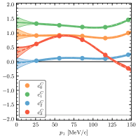
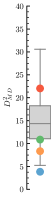
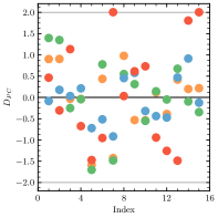
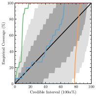
Figure 1: The Gaussian Process modeling of the current chiral expansion coefficients and its diagnostics for the EMN550 interaction. In figure (a) the simulators (solid lines - i.e. our calculation) along with the corresponding Gaussian process emulators (dashed lines) and their $2\sigma$ intervals (bands). The data used for training are denoted by dots. (b) The Mahalanobis distances compared to the mean (interior line), $50\%$ (box) and $95\%$ (whiskers) credible intervals of the reference distribution. Overall, the $D^{2}_{MD}$ are reasonably sized except for $c_{2}^{C}$. (c) The pivoted Cholesky diagnostics versus the index along with $95\%$ credible intervals (gray lines). The points seems to be distributed as expected except for the $c_{2}^{C}$ for which they show a very small variance. (d) The credible interval diagnostics for the truncation error bands. The $1(2)\sigma$ is represented with the dark(light) gray band. The flatness of the orange line up to $80\%$ CL indicates that the distance between the LO and the NLO simulation is larger than the truncation error over all the validation points indicating the over-confidence of our emulation. On the other hand, the N2LO and the N3LO are very close to each other. This generates the steep vertical green line in the figure that indicates under-confidence of our emulation in this case.

In Figure 1(a) we report the value of the coefficients $c_{n}^{C}(p_{1})$ together with the GP emulator results and their $2\sigma$ interval for the EMN550 interaction. From a first inspection, the GP emulator is able to nicely reproduce the $\chi$EFT calculation. To asses quantitatively the quality of the emulation we performed the Mahalanobis distance ($D^{2}_{MD}$) test presented in Figure 1(b), and the pivoted Cholesky decomposition ($D_{PC}$) test presented in Figure 1(c). The Mahalanobis distance test is a generalization of the squared residuals in the case of correlated data points (see Ref. Melendez et al. (2019) for more details). The comparison with the reference $\chi^{2}$ distribution shows a compatibility of the emulation with the data points within the $95\%$ CL (whiskers) for all the $c^{C}_{n}$ except for $c^{C}_{2}$ that results slightly out of the $95\%$ CL. This indicates an unusual coincidence between the emulator and the simulator (i.e. the $\chi$EFT calculation). This is evident at the level of the more informative Cholesky decomposition (see Ref. Melendez et al. (2019)). The validation points are distributed as expected for $c_{0}^{C}$, $c_{1}^{C}$ and $c_{3}^{C}$ with only a couple of points of $c_{3}^{C}$ on the line of the $2\sigma$ range. The points $c_{2}^{C}$ show an unusual density close to 0 that confirms the coincidence between the emulator and the simulator. Similar results on the two diagnostics are obtained for all the other interactions. We note only that for the NVIb and NVIIb interactions the diagnostic of $c_{3}^{C}$ improves while for the $c_{0}^{C}$ and $c_{1}^{C}$ coefficients the coincidence between the emulator and the simulator results similar to the one of $c_{3}^{C}$ for the other EM550 interaction.

In the credible interval diagnostic showed in Figure 1(d) we study if the truncation error computed at each order is compatible with the correction at the next order within a certain CL. The CL bands are constructed by sampling a large number of emulators (1000) from the underlying process. The credible intervals are then plotted against the percentage of validation points found within the interval, i.e. if the emulator contains only a small amount of the validation points is over-confident (in the figure represented as horizontal lines), in the other case is under-confident (vertical lines). For example the orange line in the Figure is the credible interval for $\Delta\Gamma_{0}^{C}(p_{1})=\Gamma^{C}_{0}(p_{1})-\Gamma^{C}_{1}(p_{1})$ compared with the reference distribution of $\delta\Gamma^{C}_{0}(p_{1})$. The credible interval for $\Delta\Gamma^{C}_{0}(p_{1})$ shows us that the emulation is over-confident regarding the first part of the spectra. That is understandable since in the low energy region the spectra is particularly steep and the difference between the LO and NLO spectra quite large (see Figure 2). At the same time the emulator for $\Delta\Gamma^{C}_{1}(p_{1})=\Gamma^{C}_{1}(p_{1})-\Gamma^{C}_{2}(p_{1})$ (in green) results under-confident since the spectra at NLO and N2LO practically coincide. On the other hand, the colored lines are in general contained in the bands which indicates a good consistency of the truncation model. The results for the confidence interval diagnostics of the other EMN interactions is practically identical. For the NV interactions the confidence interval diagnostic plot shows a better agreement between the emulator and $\Delta\Gamma^{C}_{1}(p_{1})$ and a slightly under-confidence of the emulator for $\Delta\Gamma^{C}_{2}(p_{1})=\Gamma^{C}_{2}(p_{1})-\Gamma^{C}_{3}(p_{1})$ (in blue).

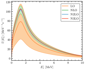
Figure 2: The differential capture rate as function of the neutron energy $E_{1}^{\prime}$ computed with the EMN550 interaction fixed at N3LO for various order of the current LO (orange), NLO (green), N2LO (blue), and N3LO (red). The bands represent the $2\sigma$ truncation errors at each order.

Since the diagnostic gave us an overall good result on the quality of the GP emulation, we computed the truncation error using Eq. (17). The order-by-order spectra obtained from the EMN550 interaction with $95\%$ CL truncation error is shown in Figure 2. Finally we compute the truncation error on the total capture rate as in Eq. (24) for each interaction. The $68\%$ CL results are reported in Table 4. Note that the integration has been performed only up to $p_{1}^{\rm max}=150$ MeV. In order to estimate the error arising from the remaining part of the spectra we used the Epelbaum et al. prescription (EP) Epelbaum et al. (2015) as considered in Ref. Ceccarelli et al. (2023). By doing so, we have found that the contribution to the total truncation error of this part of the spectra is completely negligible. Similar results have been obtained for all the other interactions.

In Table 4 we report between parentheses also the errors computed on the total capture rate using the EP exactly as in Ref. Ceccarelli et al. (2023). To give a more statistical insight, we assume that the expected decay rate is uniformly distributed within the limits settled by the extreme values and so the $68\%$ CL is given by the value of the truncation error divided by $\sqrt{3}$. As it can be seen from the table, in general the error estimated with the EP is of the same order of the one obtained using the Bayesian analysis, even if slightly smaller.

Before concluding this section, it is worthy to mention the impact the power counting of the current has on the truncation error estimate. In order to do so, we have repeated the analysis presented so far using the power counting of Ref. Ceccarelli et al. (2023), which differs from this by the fact that the axial charge and the vector current have been demoted of one order. While this clearly modifies the behavior of the coefficients $c_{n}^{C}$, it practically does not affect the value of the truncation error (both for the total and differential capture rate), neither the main conclusion of this Section.

IV.2.3 Interaction truncation errors

The other source of uncertainties we treat with the Bayesian analysis is the one arising from the truncation of the nuclear interaction chiral expansion. Unfortunately, we do not have all the orders of the NV interactions. Therefore, we limit the analysis only to the EMN interaction family. The procedure that we use is identical to the one used in the analysis of the current truncation errors. The main difference is in the factorization we use, chosen to be

$$\Gamma^{I}_{k}(p_{1})=\Gamma^{I}_{\rm ref}(p_{1})\sum_{n=0,2,3,4}c^{I}_{n}(p_{1})Q^{n}(p_{1})\,,$$ (29)

where $Q^{n}(p_{1})$ has been defined in Eq. (14) and $\Gamma^{I}_{\rm ref}(p_{1})=\Gamma^{I}_{\rm LO}(p_{1})$. This choice of the reference value makes the coefficient $c^{I}_{0}$ useless for training the emulator since it results identical to one. Therefore we exclude it in our analysis. A similar choice was done in Refs. Melendez et al. (2019); Acharya and Bacca (2022).

With respect to the previous case, we are able to extend the momentum range of the analysis up to 175 MeV. For training the emulator we use 7 points distant 25 MeV and as test point we take 19 points 9 MeV apart from each other. The nugget we used in this case is $1\times 10^{-4}$ ($2\times 10^{-4}$ for the EMN450). Note that we need a higher density of training points compared to the currents because of the large oscillations of the coefficients $c^{I}_{n}$.

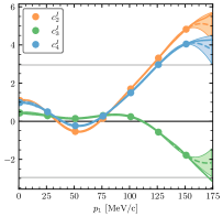
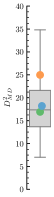
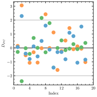
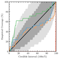
Figure 3: Same as Figure 1, but for the truncation errors of the interaction chiral expansion. The results reported in the figure are obtained using the EMN550 interaction, fixing the order of the chiral current at N2LO for the interaction at NLO, and at N3LO in the remaining cases. The red line in figure (d) represent the credible interval diagnostic of the calculation at N4LO against the truncation error computed at N3LO. The complete flatness of this line indicates that none of the validation points computed at N4LO are within the error-bars obtained at N3LO.

In Figures 3 we presents the results of the emulation together with the diagnostic performed to verify the quality of the emulation for the EMN550 interaction model. As it can be observed from the figure, both the Mahalanobis distance (Fig. 3(a)), and the pivoted Cholesky decomposition (Fig. 3(b)) confirm that the GP emulator is working properly. Similar results have been obtained for the EMN500 and EMN450 interactions.

The credible interval diagnostic shows for all the EMN interactions a compatibility of more than $95\%$ between the truncation error at given order and the prediction at the next one up to N3LO over all the empirical coverage. We have also computed the differential capture rate at N4LO and we have tested it against the truncation error computed at N3LO without including it in the Bayesian analysis. The results for the EMN550 is the red line in Figure 3(d). The fact that the empirical coverage results in a vertical line at the end of the graph tells us that there are no validation points computed at N4LO within the truncation error computed at N3LO. Similar findings have been obtained for the other two EMN interactions. Also qualitatively we observe for the total capture rate big corrections at N4LO that seem not compatible with the hypothesis of a convergent chiral expansion beyond N3LO. Since other works Melendez et al. (2019); Acharya and Bacca (2022) which use other chiral interaction models do not show this behavior at N4LO, we excluded the N4LO from our analysis.

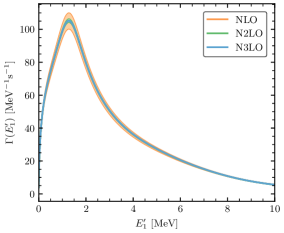
Figure 4: The differential capture rate as function of the neutron energy $E_{1}^{\prime}$ computed with the EMN550 interaction at NLO (orange), N2LO (green) and N3LO (blue). The bands represent the $2\sigma$ truncation errors at each order. Note that the chiral order of the current used in this analysis is N2LO when the interaction is at NLO and N3LO in the rest of the cases.

As for the analysis of the truncation error of the currents, we present in Figure 4 the differential capture rate spectrum computed order-by-order with the relative truncation error for the EMN550 interaction. The truncation error on the total capture rate obtained using Eq. (24) has been reported in Table 4. Once again we have verified, using the EP, that the error arising from the tail of the spectra not analyzed in the Bayesian procedure is negligible. The error obtained applying the EP over all the spectrum can be found in Table 4 between parentheses.

V Final results and discussion

We consider now the last source of uncertainty, i.e. the one arising from model dependence. Compared with previous studies, where essentially a reference value was obtained as the mean over all the interactions considered and the error was estimated as the difference between the extreme cases, we follow a slightly different approach, which allows us to give a statistical interpretation of our final result.

The truncation error on the total capture rate both for the current and the interaction has a normal distribution with standard deviation $\sigma^{C}_{k=3}$ and $\sigma^{I}_{k=4}$ respectively, as shown in Eq. (24). For the NV interaction family we take $\sigma^{I}_{k=4}=0.4$ s^-1 as in the worst case of the EMN interactions. Since the corrections to the central value ($M_{k=3}^{C}$ and $M_{k=4}^{I}$) are minimal, we assume that the two distribution have the same mean, i.e.

$$\Gamma(\infty)=\Gamma({\rm comp})+M_{k=3}^{C}+M_{k=4}^{I}\,.$$ (30)

We can assume that the final probability distribution for the total capture rate generated by the error on the current LECs is a normal distribution with the mean defined in Eq. (30) and a standard deviation given by $\sigma_{\rm LECs}$. If we consider the three sources of error as independent, it is easy to verify that the overall distribution is given by

$$\Gamma_{i}\sim\mathcal{N}[\Gamma_{i}(\infty),\sigma_{i}]\ ,$$ (31)

where with $i$ we indicate the interaction used, $\Gamma_{i}(\infty)$ is defined in Eq. (30), and

$$\sigma_{i}=\sqrt{(\sigma^{C}_{i,k=3})^{2}+(\sigma^{I}_{i,k=4})^{2}+\sigma_{i,{\rm LECs}}^{2}}\,.$$ (32)

In the space of the phase shifts equivalent chiral interactions, we can assume that all of them are equivalent. Therefore, we construct the density probability for our final result $\Gamma_{\rm th}$ by choosing randomly one of the interactions and then sampling a point from the $\Gamma_{i}$ distribution of the selected one. We repeat this operation for $10^{5}$ times constructing the final distribution of $\Gamma$. By chance this has the shape of a Normal distribution with mean $393.8$ s^-1 and standard deviation $4.4$ s^-1. Therefore, our recommended value for the total capture rate at N3LO is

$$\Gamma_{\rm th}=(393.8\pm 4.4)\,{\rm s}^{-1}\quad(68\%{\rm CL})\,.$$ (33)

An identical analysis have been performed on the differential capture rate for each value of $E_{1}^{\prime}$. Our recommended spectra is shown in Figure 5 with the bands at $68\%$, $95\%$, and $99\%$ CLs. A Table of the final spectra is provided as supplementary material sup . To be remarked that the differences among the three CLs can be appreciated only at the peak of the spectra.

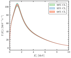
Figure 5: The recommended differential capture rate as function of the neutron energy $E_{1}^{\prime}$. The green, blue, and red bands represent respectively the 99$\%$, 95$\%$, and $68\%$ CL. Note that the difference among the bands can be appreciated only at the peak of the spectra.

The comparison of our results with those present in the literature still obtained within $\chi$EFT can be seen in Figure 6. By inspection of the figure we can conclude that despite the central value depends slightly on the interactions used in the analysis, the most recent calculations are all compatible within $1\sigma$ with our result. Note that for the previous calculations we have assumed that the errors represent the extreme of a uniform distribution. For Ref. Adam et al. (2012), we have considered as limit of the distribution the minimal and the maximal reported results. Therefore, in Figure 6 we report the error divided for $\sqrt{3}$, in order to obtain the $68\%$ CL. The central value of our result is slightly smaller than those in literature mainly, because of the small value obtained with the EMN450 interaction. It is worthy to mention that if we were going to exclude the EMN450 interaction, our results would be in reasonable agreement with the one obtained using the NNLOsim interaction in Ref. Bonilla et al. (2023). Note also that only in our work and in Ref. Bonilla et al. (2023) the error includes the uncertainty on $r_{A}^{2}$. We do not proceed in comparing our results with the available experimental data of Refs. Wang et al. (1965); Bertin et al. (1973); Bardin et al. (1986); Cargnelli M, et al. (1989), because of their large uncertainties.

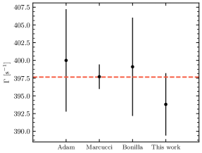
Figure 6: Comparison of the theoretical results obtained within $\chi$EFT in recent works Adam et al. (2012); Marcucci et al. (2012); Bonilla et al. (2023). The errors in the previous works have been assumed to be the limit of a uniform distribution and then divided by $\sqrt{3}$ to obtain the $68\%$ CL. Note that only in Ref. Bonilla et al. (2023) and in the present work various sources of uncertainty besides the model dependence were considered. The red dashed line represent the arithmetic mean of the theoretical results.

In order to appreciate the importance of the various uncertainty sources in the total error budget, we list in Table 5 their relative weight in percentage. As final consideration, we want to remark that our analysis showed that the theoretical error is dominated by the $r_{A}^{2}$ uncertainty if both the interactions and the currents are considered at N3LO. The model dependence slightly increases the variance of the Gaussian distribution, but it is not significant with respect to the uncertainty on $r_{A}^{2}$. If we had stopped our calculation at N2LO, the truncation error at $68\%$ CL would have been between $3.3$ and $6.5$ s^-1 for the currents, and $\sim 1.5$ s^-1 for the interactions. Note that the truncation error obtained here at N2LO is of the same order as the truncation error estimated at N2LO in Ref. Bonilla et al. (2023), using the prescription of Ref. Furnstahl et al. (2015), once properly rescaled for the different value of $\Lambda_{b}$ used in our work. Combining our results for the truncation error at N2LO with the error on $r_{A}^{2}$ as before we obtain a total error of $6.8$ s^-1 (68$\%$ CL).

Uncertainty source	Impact
$r_{A}^{2}$	$78.5\%$
Other current LECs	negligible
$\chi$EFT truncation - currents	$5.2\%$
$\chi$EFT truncation - interactions	$0.8\%$
Model dependence	$15.5\%$

Table 5: Relative contributions to the estimated total theoretical error from the various uncertainty sources.

VI Impact on the MUSUN experiment

In this Section we present a minimal study of the impact of our results in the analysis of the future experimental results of MuSun. For our analysis we assume that the final error of the experiment is the expected precision of $\sim 1.5\%$ P. Kammel on behalf of the MuSun collaboration (2021). Since this is just a preliminary analysis we consider only the nuclear interaction NVIa and the error associated to this interaction reported in the first line of Table 4.

First we study the dependence of the total capture rate as function of the value of the LEC $c_{D}$ from which $z_{0}$ depends linearly. For this analysis we fixed the value of $r_{A}^{2}=0.46$ without considering the impact of the error associated with $r_{A}^{2}$. As it can be seen in Figure 7 the dependence of $\Gamma$ on $c_{D}$ is linear but with a very small inclination. The red dashed lines represent the error generated on $\Gamma$ from the uncertainty on $c_{D}$. As it can be seen, even if the uncertainty on $c_{D}$ is large the impact on $\Gamma$ is minimal ($\sim 0.3\%$). A 1.5% precision on the experimental results would correspond to a very large set of values of $c_{D}$ much larger than the present constrains, even without considering the uncertainty on $r_{A}^{2}$ that would make the case even worst.

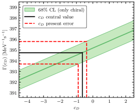
Figure 7: Capture rate as function of the value of $c_{D}$ for the NVIa interaction. The green band represent the error on $\Gamma$ due to the truncation error on the chiral expansion of the current and the interaction. The red dashed lines represent the $68\%$ CL on $\Gamma$ considering the error on $c_{D}$ as reported in Ref. Baroni et al. (2018).

On the other hand, we can perform a similar analysis varying $r_{A}^{2}$. In this case for simplicity we keep $c_{D}$ fixed. In Figure  8 we plot the the capture rate as function of $r_{A}^{2}$ for the NVIa interaction. The red dashed lines represents the present uncertainty on $r_{A}^{2}$ that generate an uncertainty on $\Gamma$ of the order of $\sim 1\%$. To improve the uncertainty on $r_{A}^{2}$ at the order of $10\%$ a rough estimate indicate that we would need a precision of the order of $0.6\%$ on the experimental data.

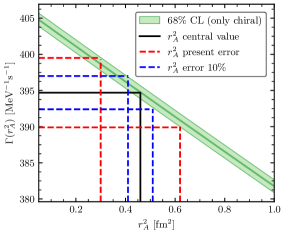
Figure 8: Capture rate as function of the value of $r_{A}^{2}$ for the NVIa interaction. The green band represent the error on $\Gamma$ due to the truncation error on the chiral expansion of the current and the interaction. The red dashed lines represent the $68\%$ CL on $\Gamma$ considering the error on $r_{A}^{2}$ as reported in Ref. Hill et al. (2018). The blue dashed lines represent the predicted $68\%$ CL on $\Gamma$ with an error of $10\%$ on $r_{A}^{2}$.

While this analysis shows the difficulties of extracting precision values for $c_{D}$ and $r_{A}^{2}$ from the MuSun experiment with the present previsions on the uncertainty, we want to remark that the results of the MuSun experiment are still a fundamental test for the parameters of chiral effective field theory. Indeed, MuSun will be the first precise measurement of the rate for a weak process in the two-nucleon system, which can be compared with theoretical predictions accompanied by fully quantified uncertainties. Any strong deviation of the experimental results or inconsistency with the present literature would imply the necessity of a profound revision for the chiral electroweak currents. Furthermore, we would like to stress that the MuSun experiment remains one of the best options to access with good accuracy the LEC $L_{1A}$ present (see for example the work of Chen et al. Chen et al. (2005)), within pionless EFT, in several two-nucleon processes, among which, besides muon capture, also the proton-proton fusion reaction, of paramount importance in astrophysics.

References

- Wang et al. (1965) I. T. Wang, E. W. Anderson, E. J. Bleser, L. M. Lederman, S. L. Meyer, J. L. Rosen, and J. E. Rothberg, Phys. Rev. 139, B1528 (1965).
- Bertin et al. (1973) A. Bertin, A. Vitale, A. Placci, and E. Zavattini, Phys. Rev. D 8, 3774 (1973).
- Bardin et al. (1986) G. Bardin, J. Duclos, J. Martino, A. Bertin, M. Capponi, M. Piccinini, and A. Vitale, Nucl. Phys. A 453, 591 (1986).
- Cargnelli M, et al. (1989) Cargnelli M, et al., Nuclear weak process and nuclear structure, Yamada Conference XXIII, edited by M. Morita, H. Ejiri, H. Ohtsubo, and T. Sato, World Scientific, Singapore , 115 (1989).
- P. Kammel on behalf of the MuSun collaboration (2021) P. Kammel on behalf of the MuSun collaboration, SciPost Phys. Proc. , 018 (2021).
- Marcucci (2012) L. E. Marcucci, Int. J. Mod. Phys. A 27, 1230006 (2012).
- Marcucci et al. (2011) L. E. Marcucci, M. Piarulli, M. Viviani, L. Girlanda, A. Kievsky, S. Rosati, and R. Schiavilla, Phys. Rev. C 83, 014002 (2011).
- Golak et al. (2014) J. Golak, R. Skibiński, H. Witała, K. Topolnicki, A. E. Elmeshneb, H. Kamada, A. Nogga, and L. E. Marcucci, Phys. Rev. C 90, 024001 (2014), [Addendum: Phys. Rev. C 90, 029904 (2014)].
- Ando et al. (2002) S. Ando, T.-S. Park, K. Kubodera, and F. Myhrer, Physics Letters B 533, 25 (2002).
- Marcucci et al. (2012) L. E. Marcucci, A. Kievsky, S. Rosati, R. Schiavilla, and M. Viviani, Phys. Rev. Lett. 108, 052502 (2012), [Erratum: Phys. Rev. Lett. 121, (2018) 049901].
- Adam et al. (2012) J. Adam, Jr., M. Tater, E. Truhlik, E. Epelbaum, R. Machleidt, and P. Ricci, Phys. Lett. B 709, 93 (2012).
- Marcucci et al. (2020) L. E. Marcucci, J. Dohet-Eraly, L. Girlanda, A. Gnech, A. Kievsky, and M. Viviani, Front. Phys. 8, 69 (2020).
- Acharya et al. (2018) B. Acharya, A. Ekström, and L. Platter, Phys. Rev. C 98, 065506 (2018).
- Hill et al. (2018) R. J. Hill, P. Kammel, W. J. Marciano, and A. Sirlin, Rep. Prog. Phys. 81, 096301 (2018).
- Bonilla et al. (2023) J. Bonilla, B. Acharya, and L. Platter, arXiv:2212.08138 (2023).
- Ceccarelli et al. (2023) L. Ceccarelli, A. Gnech, L. E. Marcucci, M. Piarulli, and M. Viviani, Frontiers in Physics 10 (2023), 10.3389/fphy.2022.1049919.
- Melendez et al. (2019) J. A. Melendez, R. J. Furnstahl, D. R. Phillips, M. T. Pratola, and S. Wesolowski, Phys. Rev. C 100, 044001 (2019).
- (18) “Buqeye collaboration,” https://buqeye.github.io/publications/.
- Andreev et al. (2010) V. A. Andreev, R. M. Carey, V. A. Ganzha, A. Gardestig, T. P. Gorringe, F. Gray, D. W. Hertzog, M. Hildebrandt, P. Kammel, B. Kiburg, S. Knaack, P. Kravtsov, A. Krivshich, K. Kubodera, B. Lauss, K. R. Lynch, E. Maev, O. Maev, F. Mulhauser, F. Myhrer, C. Petitjean, G. E. Petrov, R. Prieels, G. N. Schapkin, G. G. Semenchuk, M. A. Soroka, V. Tishchenko, A. A. Vasilyev, A. Vorobyov, M. Vznuzdaev, and P. Winter, arXiv:1004.1754 (2010).
- Kohn (1948) W. Kohn, Phys. Rev. 74, 1763 (1948).
- Walecka (1995) J. Walecka, Theorethical Nuclear and Subnuclear Physics (Imperial College Press, London, 1995).
- Hardy and Towner (2020) J. C. Hardy and I. S. Towner, Phys. Rev. C 102, 045501 (2020).
- Piarulli et al. (2015) M. Piarulli, L. Girlanda, R. Schiavilla, R. N. Pérez, J. E. Amaro, and E. R. Arriola, Phys. Rev. C 91, 024003 (2015).
- Piarulli et al. (2016) M. Piarulli, L. Girlanda, R. Schiavilla, A. Kievsky, A. Lovato, L. E. Marcucci, S. C. Pieper, M. Viviani, and R. B. Wiringa, Phys. Rev. C 94, 054007 (2016).
- Entem et al. (2017) D. R. Entem, R. Machleidt, and Y. Nosyk, Phys. Rev. C 96, 024004 (2017).
- Baroni et al. (2016) A. Baroni, L. Girlanda, S. Pastore, R. Schiavilla, and M. Viviani, Phys. Rev. C 93, 015501 (2016).
- Baroni et al. (2018) A. Baroni, R. Schiavilla, L. E. Marcucci, L. Girlanda, A. Kievsky, A. Lovato, S. Pastore, M. Piarulli, S. C. Pieper, M. Viviani, and R. B. Wiringa, Phys. Rev. C 98, 044003 (2018).
- Pastore et al. (2009) S. Pastore, L. Girlanda, R. Schiavilla, M. Viviani, and R. B. Wiringa, Phys. Rev. C 80, 034004 (2009).
- Piarulli et al. (2013) M. Piarulli, L. Girlanda, L. E. Marcucci, S. Pastore, R. Schiavilla, and M. Viviani, Phys. Rev. C 87, 014006 (2013).
- Marcucci et al. (2019) L. E. Marcucci, F. Sammarruca, M. Viviani, and R. Machleidt, Phys. Rev. C 99, 034003 (2019).
- Gnech and Schiavilla (2022) A. Gnech and R. Schiavilla, Phys. Rev. C 106, 044001 (2022).
- Epelbaum et al. (2015) E. Epelbaum, H. Krebs, and U.-G. Meissner, Eur. Phys. J. A 51, 53 (2015).
- Patrignani (2016) C. Patrignani, Chinese Physics C 40, 100001 (2016).
- Acharya and Bacca (2022) B. Acharya and S. Bacca, Phys. Lett. B 827, 137011 (2022).
- (35) “See supplemental material at for the differential muon capture rate on deuteron.” .
- Furnstahl et al. (2015) R. J. Furnstahl, N. Klco, D. R. Phillips, and S. Wesolowski, Phys. Rev. C 92, 024005 (2015).
- Chen et al. (2005) J.-W. Chen, T. Inoue, X. Ji, and Y. Li, Phys. Rev. C 72, 061001 (2005).