A discrete Blaschke Theorem for convex polygons in $2$-dimensional space forms

Abstract

Let $M$ be a $2$-space form. Let $P$ be a convex polygon in $M$. For these polygons, we define (and justify) a curvature ${\kappa}_{i}$ at each vertex $A_{i}$ of the polygon and and prove the following Blaschke’s type theorem: “If $P$ is a convex plygon in $M$ with curvature at its vertices ${\kappa}_{i}\geq{\kappa}_{0}>0$, then the circumradius $R$ of $P$ satisfies ${\rm ta_{\lambda}}(R)\leq\pi/(2{\kappa}_{0})$ and the equality holds if and only if the polygon is a $2$-covered segment”

1 Introduction and main result

We start recalling that a $n$-dimensional space form ${\overline{M}_{\lambda}^{n+1}}$ of curvature $\lambda$ is a simply connected $n$-dimensional Riemannian manifold of constant sectional curvature $\lambda$. The only ones are: when $\lambda=0$, the Euclidean Space, when $\lambda>0$, the $n$-dimensional sphere of radius $1/\sqrt{\lambda}$ in the euclidean $\mathbb{R}^{n+1}$, and, when $\lambda<0$, the Hyperbolic Space of sectional curvature $\lambda$, that can be visualized as the upper connected component of the Minkowski sphere of radius $1/\sqrt{|\lambda|}$ in the Minkowski Space $\mathbb{R}^{n+1}$.

In the book of Blaschke [1] it is proved that if $\Gamma$ is a closed convex regular curve in the Euclidean plane that bounds a compact convex region $\Omega$ and the curvature ${\kappa}$ of $\Gamma$ is bounded from below by some constant ${\kappa}_{0}>0$, then, for every point $p\in\Gamma$, the circle tangent to $\Gamma$ at $p$ and with radius $R=\displaystyle\frac{1}{{\kappa}_{0}}$ bounds a disk that contains $\Omega$.

This result was extended by H. Karcher ([8]) for the other space forms. Before stating it, we recall a notation that allows to describe the geometry of space forms can be described in a unified way:

$${\rm s_{\lambda}}(t)=\begin{cases}\frac{\sin(\sqrt{\lambda}t)}{\sqrt{\lambda}},&\text{ if }\lambda>0\\ t&\text{ if }\lambda=0\\ \frac{\sinh(\sqrt{|\lambda|}t)}{\sqrt{|\lambda|}}&\text{ if }\lambda<0\end{cases},\quad\begin{array}[]{c}{\rm c_{\lambda}}(t)=\begin{cases}\cos(\sqrt{\lambda}t),&\text{ if }\lambda>0\\ 1&\text{ if }\lambda=0\\ \cosh(\sqrt{|\lambda|}t)&\text{ if }\lambda<0\end{cases},\\ {\rm ta_{\lambda}}(t)=\displaystyle\frac{{\rm s_{\lambda}}(t)}{{\rm c_{\lambda}}(t)},\quad\text{and}\quad{\rm co_{\lambda}}(t)=\displaystyle\frac{{\rm c_{\lambda}}(t)}{{\rm s_{\lambda}}(t)}\end{array}.$$ (1)

The functions above satisfy the following computational rules:

$${\rm c}^{\prime}_{\lambda}=-\lambda\,{\rm s_{\lambda}},\quad{\rm s_{\lambda}}^{\prime}(t)={\rm c_{\lambda}}(t),\quad{\rm c}^{2}_{\lambda}+\lambda\,{\rm s}^{2}_{\lambda}=1,\quad\quad\frac{1}{{\rm c_{\lambda}}^{2}(t)}=1+\lambda{\rm ta_{\lambda}}^{2}(t),$$ (2)

$${\rm s_{\lambda}}(t+u)={\rm s_{\lambda}}(t){\rm c_{\lambda}}(u)+{\rm c_{\lambda}}(t){\rm s_{\lambda}}(u)\text{ and }{\rm c_{\lambda}}(t+u)={\rm c_{\lambda}}(t){\rm c_{\lambda}}(u)-\lambda\ {\rm s_{\lambda}}(t){\rm s_{\lambda}}(u).$$

where “ ^′ ”denotes the derivative respect to $t$.

We shall recall also the following concept:

Given any convex closed curve $\Gamma$ in ${\overline{M}_{\lambda}^{2}}$, the circumradius of $\Gamma$ is the minimum value of $R$ such that a disk of radius $R$ in ${\overline{M}_{\lambda}^{2}}$ contains the domain bounded by $\Gamma$.

With this concept, the Blaschke-Karcher theorem can be stated in the following form:

     Theorem 1 ([8]).

if $\Gamma$ is a closed convex $C^{2}$ curve in ${\overline{M}_{\lambda}^{2}}$ that bounds a compact convex region $\Omega$ and with curvature ${\kappa}$ (where it is $C^{2}$) satisfies ${\kappa}\geq{\kappa}_{0}>\max\{0,-\lambda\}$, then the circumradius $R$ of $\Gamma$ satisfies ${\rm ta_{\lambda}}(R)\leq\displaystyle\frac{1}{{\kappa}_{0}}$.

Further developments of related Blaschke theorems has been done by obtaining conditions under which a convex set in $\mathbb{R}^{n}$ can be included in other ([10, 6, 4]) or its generalization to Riemannian manifolds where the included convex is a sphere ([7]).

In Theorem 1 (and in the other cited developments), the hypothesis of strong convexity (${\kappa}\geq{\kappa}_{0}>0$) is necessary, the theorem is not true for ${\kappa}\geq 0$. Then it cannot be applied to closed convex polygons. Here we shall show that it is possible to have a version of the theorem for polygons once we give an appropriate definition of curvature at the vertices of a polygon. We shall take the following one:

     Definition 1.

Let $A$ be a vertex of a convex polygon $P$ in a space form ${\overline{M}_{\lambda}^{2}}$. When $\lambda>0$, the sides $\ell_{i}$ of $P$ must satisfy $\ell_{i}<\pi/\sqrt{\lambda}$. Let ${\widehat{A}}$ be the interior angle of $P$ at the vertex $A$, and let $\ell_{1},\ell_{2}$ be the lengths of the sides of $P$ that meet at vertex $A$. We define the “curvature of $P$ at $A$”by the number

$${\kappa}_{A}=\frac{(\pi-{\widehat{A}})}{{\rm ta_{\lambda}}(\ell_{1}/2)+{\rm ta_{\lambda}}(\ell_{2}/2)}.$$ (3)

A compact convex polygon $P$ is called ${\kappa}_{0}$-convex if at every vertex $A$ of $P$, ${\kappa}_{A}\geq{\kappa}_{0}>0$.

When $$\lambda=0 {\kappa}_{A}=\displaystyle\frac{2(\pi-{\widehat{A}})}{\ell_{1}+\ell_{2}}$$, the definition (3) becomes . (4)

In the next section we shall give the reasons why we have chosen Definition (3).

The version of Theorem 1 that shall prove for polygons is:

     Theorem 2.

Let $P$ be a compact ${\kappa}_{0}$-convex polygon in ${\overline{M}_{\lambda}^{2}}$, with sides lower than $\pi/\sqrt{\lambda}$ if $\lambda>0$, and with curvature at each vertex $A_{i}$ satisfying ${\kappa}_{A_{i}}\geq{\kappa}_{0}>\max\{0,-\lambda\}$. Then the circumradius $R$ of $P$ satisfies

$${\rm ta_{\lambda}}(R)\leq\pi/(2{\kappa}_{0}),$$ (5)

and the equality holds if and only if the polygon degenerates to a $2$-covered segment.

For the euclidean plane, Definition (4) was used in [2] in the study of approximations of surfaces by planar triangulations and in [3] it was studied how good is this definition to approximate the curvature of a planar curve by a polygonal line. Other applications of this definition in the euclidean case has been done in [5]. Related but different definitions of curvature of a polygon in the euclidean plane have been used for other applications in [9] and [11].

Some people could prefer to take (4) as definition for the curvature of a convex polygon for every ${\overline{M}_{\lambda}^{2}}$, without having into account the value of $\lambda$. In the last section of the paper we shall give the corresponding result (Th. 4) for this definition.

2 About Definition 1

If we consider a convex polygon as a limit of smooth curves approaching it and the curvature at a vertex as the limit of the curvature of the points at the curves whose limit is the vertex, then the curvature becomes infinite. Obviously, this is not a good definition for many geometric properties. We would like a definition satisfying the following properties:

• the curvature of a vertex is bigger as the interior angle is lower

• the curvature of a vertex is bigger as the lengths of the adjacent sides is shorter

• if we have a regular polygon inscribed in a circle and we take the number of sides of the regular polygon increasing up to infinite, the curvature of the vertices approach the curvature of the circle.

Properties P1 and P3 correspond to a natural geometric intuition. Property P2 is related to the fact that we want to generalize Theorem 1 which fails when ${\kappa}_{0}=0$ (in the Euclidean case) because with ${\kappa}_{0}=0$ you may have straight lines with arbitrary length which are the obstacle for upper bounds for the circumradius.

It is obvious that our definition 1 satisfies P1 and P2. In the next Proposition, we shall check that it also satisfies P3.

     Proposition 3.

Let $C$ be a circle of radius $R$ ($<\pi/(2\sqrt{\lambda})$ if $\lambda>0$) in ${\overline{M}_{\lambda}^{2}}$ and let $P_{n}$ be a regular polygon of $n$ sides with its vertices in $C$. If ${\kappa}_{n}$ denotes the specific curvature at any vertex $A_{n}$ of the polygon $P_{n}$, then $\lim_{n\to\infty}{\kappa}_{n}={\rm co_{\lambda}}(R)$, which is the curvature of $C$.

Proof Let us recall some trigonometric formulae of the space forms: Let $\Delta$ be a geodesic triangle with sides $a,b,c$ and opposite vertices $A,B,C$. Let ${\widehat{A}},{\widehat{\rm B}},{\widehat{C}}$ be the angles at these vertices. Then the following formulae hold:

$$\cos{\widehat{A}} =\frac{{\rm c_{\lambda}}(a)-{\rm c_{\lambda}}(b)\ {\rm c_{\lambda}}(c)}{\lambda\ {\rm s_{\lambda}}(b)\ {\rm s_{\lambda}}(c)}$$ (6)

$$(\text{when } \lambda=0\text{ the quotient in the second term of \eqref{ca} must be understood}$$

taking $$\text{ limits for }\lambda\to 0,\text{giving the standard cosinus law in Euclidean plane})$$

$$\frac{\sin{\widehat{A}}}{{\rm s_{\lambda}}(a)} =\frac{\sin{\widehat{\rm B}}}{{\rm s_{\lambda}}(b)}=\frac{\sin{\widehat{C}}}{{\rm s_{\lambda}}(c)}$$ (7)

Let $A_{n}$, $B_{n}$ be two consecutive vertices of the polygon, bounding a side $A_{n}B_{n}$ of length $\ell_{n}$. Let $M_{n}$ be the middle point of $A_{n}B_{n}$ between $A_{n}$ and $B_{n}$. Let $O$ be the center of the circle. Let us consider the geodesic triangle $OM_{n}B_{n}$, and denote by $d_{n}$ the length of the geodesic $OM_{n}$. One has ${\widehat{M}}_{n}=\pi/2$. We can apply (6) and (7) to this triangle to obtain:

$${\rm c_{\lambda}}(R) ={\rm c_{\lambda}}(d_{n}){\rm c_{\lambda}}(\ell_{n}/2),\qquad{\rm s_{\lambda}}(d_{n})={\rm s_{\lambda}}(R)\sin({\widehat{\rm B}}_{n}/2)$$

From these two equalities and the formulae (2) we obtain

$$\frac{{\rm c_{\lambda}}^{2}(R)}{{\rm c_{\lambda}}^{2}(\ell_{n}/2)}={\rm c_{\lambda}}^{2}(d_{n})=1-\lambda{\rm s_{\lambda}}^{2}(d_{n})=1-\lambda\ {\rm s_{\lambda}}^{2}(R)\sin^{2}({\widehat{\rm B}}_{n}/2)\text{, then }$$

$$\sin^{2}({\widehat{\rm B}}_{n}/2)=\frac{1}{\lambda\ {\rm s_{\lambda}}^{2}(R)}-\frac{{\rm co_{\lambda}}^{2}(R)}{\lambda\ {\rm c_{\lambda}}^{2}(\ell_{n}/2)}=1+\frac{{\rm co_{\lambda}}^{2}(R)}{\lambda}\left(1-\frac{1}{{\rm c_{\lambda}}^{2}(\ell_{n}/2)}\right)$$

$$\cos^{2}(({\widehat{\rm B}}_{n}/2)=1-\sin^{2}({\widehat{\rm B}}_{n}/2)={\rm co_{\lambda}}^{2}(R){\rm ta_{\lambda}}^{2}(\ell_{n}/2),\text{ then}$$

$${\rm ta_{\lambda}}(\ell_{n}/2)={\rm ta_{\lambda}}(R)\cos({\widehat{\rm B}}_{n}/2)={\rm ta_{\lambda}}(R)\sin(\pi/2-{\widehat{\rm B}}_{n}/2)$$ (8)

We apply now the definition (3) to the curvature $\mathfrak{k}_{n}$ of ${\widehat{\rm B}}_{n}$

$${\kappa}_{n}=\frac{(\pi-{\widehat{\rm B}}_{n})}{2{\rm ta_{\lambda}}(\ell_{n}/2)}=\frac{2(\pi/2-{\widehat{\rm B}}_{n}/2)}{2{\rm ta_{\lambda}}(R)\sin(\pi/2-{\widehat{\rm B}}_{n}/2)}.$$ (9)

But $\lim_{n\to\infty}{\widehat{\rm B}}_{n}=\pi$, then the limit of the quotient in (9) for $n\to\infty$ is ${\rm co_{\lambda}}(R)$, as claimed in Prop. 3. ∎

Definition 1 is not the unique satisfying properties P1 to P3. If we take (4) as a definition of the curvature at $A$ for any value of $\lambda$, it is obvious that it satisfies P1 and P2, moreover P3 follows with the same proof of Proposition 3 , having into account that $\lim_{n\to\infty}\frac{{\rm ta_{\lambda}}(\ell_{n}/2)}{(\ell_{n}/2)}=1$. We have preferred (3) because it gives a clean bound (5) in Theorem 2, but some people could prefer the other definition.

3 Proof of the Theorem

Let $A_{1},A_{2},...,A_{n}$ be the consecutive vertices of the polygon $P$. Let $\hat{A}_{i}$ be the angles at these vertices, and $\ell_{1},...,\ell_{i},...,\ell_{n}$ be the lengths of the sides $A_{n}A_{1},...,A_{i-1}A_{i},...,A_{n-1}A_{n}$ respectively (see Figure 1).

For every segment $A_{i-1}A_{i}$ we construct a segment of circle $C_{i}$ of radius $\rho_{i}$ with center $O_{i}$ in a line orthogonal to $A_{i-1}A_{i}$ in its middle point and in the ray in the inward direction, and with boundary points $A_{i}$ and $A_{i+1}$.

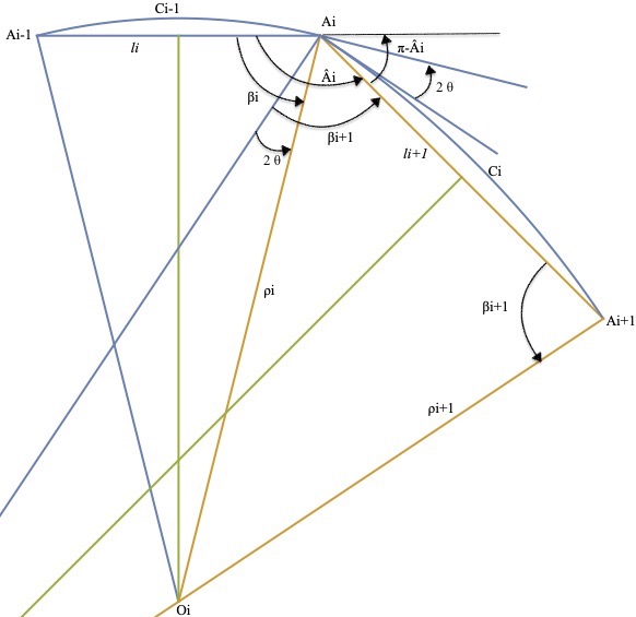
Figure 1:

Each angle $\beta_{i}$ at $A_{i}$ of the isosceles triangle $A_{i-1}A_{i}O_{i}$ satisfies $0<\beta_{i}<\pi/2$ and the analogous of (8) for this triangle is

$${\rm ta_{\lambda}}(\ell_{i}/2)={\rm ta_{\lambda}}(\rho_{i})\cos\beta_{i}={\rm ta_{\lambda}}(\rho_{i})\sin(\delta_{i})$$ (10)

if we take $\delta_{i}=\pi/2-\beta_{i}$.

We now take the curve obtained as the union of the segments of circle $C_{i}$. This curve will be convex if and only if, for every $i=1,..,n$, the tangent vectors at $A_{i}$ of the circles $C_{i-1}$ and $C_{i}$ with the curve $C_{i-1}$ oriented from $A_{i-1}$ to $A_{i}$ and the curve $C_{i}$ oriented from $A_{i}$ to $A_{i+1}$ form an angle $2\ \theta_{i}$ in the interval $[0,\pi]$. This angle is the same that the one formed by the normals at $A_{i}$ to $C_{i-1}$ and $C_{i}$ pointing inward. These normals are $A_{i}O_{i}$ and $A_{i}O_{i+1}$, and this angle is non negative if and only if $\beta_{i}+\beta_{i+1}\geq\hat{A}_{i}$, that is $\pi-\delta_{i}-\delta_{i+1}\geq\pi-(\pi-\hat{A}_{i})$,

$$\delta_{i}+\delta_{i+1}\leq\pi-\hat{A}_{i}.$$ (11)

For every $i$, let us choose $\rho_{i}=R$ such that ${\rm ta_{\lambda}}(R)=\frac{c}{{\kappa}_{0}}$. From the hypothesis of ${\kappa}_{0}$-convexity of $P$, and using formula (10), we have

$${\kappa}_{0}\leq \frac{\pi-\hat{A}_{i}}{{\rm ta_{\lambda}}(\ell_{i}/2)+{\rm ta_{\lambda}}(\ell_{i+1}/2)}=\frac{(\pi-\hat{A}_{i})}{{\rm ta_{\lambda}}(\rho_{i})\sin\delta_{i}+{\rm ta_{\lambda}}(\rho_{i+1})\sin\delta_{i+1}}=\frac{{\kappa}_{0}}{c}\ \frac{(\pi-\hat{A}_{i})}{\sin\delta_{i}+\sin\delta_{i+1}},$$

then $$\pi-\hat{A}_{i}\geq c\ (\sin\delta_{i}+\sin\delta_{i+1})\geq c\frac{2}{\pi}\ (\delta_{i}+\delta_{i+1})$$ (12)

an inequality which coincides with (11) if $c=\pi/2$, which gives ${\rm ta_{\lambda}}(\rho_{i})={\rm ta_{\lambda}}(R)=\displaystyle\frac{\pi}{2\ {\kappa}_{0}}$. As a consequence the closed curve $C$ formed by the union of the $C_{i}$ is convex and with curvature equal $\displaystyle\frac{2{\kappa}_{0}}{\pi}$ at every regular point. Now, for every $i$, let us take the exterior parallel curve $C_{i\varepsilon}$ at distance $\varepsilon$ from $C_{i}$. Each $C_{i\varepsilon}$ is an arc of circle of radius $R+\varepsilon$, then it has curvature

$${\kappa}_{i}={\rm co_{\lambda}}(R+\varepsilon)=\displaystyle\frac{{\rm co_{\lambda}}(R)+\lambda{\rm ta_{\lambda}}(\varepsilon)}{1-{\rm co_{\lambda}}(R){\rm ta_{\lambda}}(\varepsilon)}=\displaystyle\frac{2{\kappa}_{0}/\pi+\lambda{\rm ta_{\lambda}}(\varepsilon)}{1-{\rm ta_{\lambda}}(\varepsilon)2{\kappa}_{0}/\pi}.$$

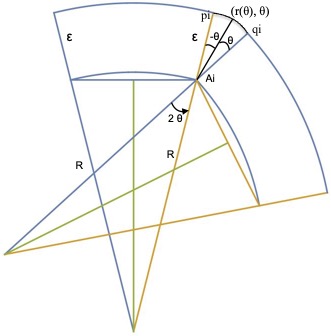
Figure 2:

Given to consecutive arcs $C_{\varepsilon i-1}$ and $C_{\varepsilon i}$, we join the right extreme $p_{i}$ of $C_{\varepsilon i-1}$ with the left extreme $q_{i}$ of $C_{\varepsilon i}$ by a curve that, in polar geodesic coordinates $(r,\varphi)$ around $A_{i}$ has the expression $c_{i}(\varphi)=(r_{i}(\varphi),\varphi)$, with $-\theta_{i}\leq\varphi\leq\theta_{i}$ (see Figure 2), satisfying

$$p_{i} =c_{i}(-\theta_{i})=(r_{i}(-\theta_{i}),-\theta_{i}),\quad q_{i}=c_{i}(\theta_{i})=(r_{i}(\theta_{i}),\theta_{i})$$

$$\text{ that is }\quad r_{i}(-\theta_{i})=\varepsilon=r_{i}(\theta_{i})$$ (13)

$$c_{i}^{\prime}(-\theta_{i}) \text{ is tangent to }C_{(i-1)\varepsilon}\text{ at }p_{i}\text{ and }c_{i}^{\prime}(\theta_{i})\text{ is tangent to }C_{i\varepsilon}\text{ at }q_{i}$$

$$\text{that is }r_{i}^{\prime}(-\theta_{i})=0=r_{i}^{\prime}(\theta_{i})$$ (14)

the curvature $$k_{i} c_{i}\text{ at }c_{i}(-\theta_{i})\text{ is equal to the curvature of }C_{(i-1)\varepsilon}\text{ at }p_{i}\text{ and }$$ of

the curvature $$k_{i} c_{i}\text{ at }c_{i}(\theta_{i})\text{ is equal to the curvature of }C_{i\varepsilon}\text{ at }p_{i}$$ of

$$\text{that is }k_{i}(-\theta_{i})={\kappa}_{i}={\rm co_{\lambda}}(R+r)=k_{i}(\theta_{i}).$$ (15)

With these conditions, the curve $C_{\varepsilon}$ obtained joining all the curves $C_{i\varepsilon}$ and $c_{i}$ is $C^{2}$. Moreover, the function $r_{i}(\varphi)$ can be taken (see the appendix) such that,

$$\lim_{\varepsilon\to 0^{+}}k_{i}(\varphi)=\infty\quad\text{for }-\theta_{i}<\varphi<\theta_{i},$$ (16)

then for small enough $\varepsilon$, $k_{i}>{\rm co_{\lambda}}(R+\varepsilon)$, then the curve $C_{\varepsilon}$ has curvature bigger than $2\ {\kappa}_{0}/\pi+\psi(\varepsilon)$ with $\psi(\varepsilon)=\displaystyle\frac{2{\kappa}_{0}+\lambda\pi^{2}}{\pi^{2}-\pi{\rm ta_{\lambda}}(\varepsilon)2{\kappa}_{0}}{\rm ta_{\lambda}}(\varepsilon),$ then $\lim_{\varepsilon\to 0}\psi(\varepsilon)=0$.

To each one of these curves $C_{\varepsilon}$ we can apply Theorem 1 and conclude that the circumradius $R_{\varepsilon}$ of each one of them satisfies ${\rm ta_{\lambda}}(R_{\varepsilon})\leq\displaystyle\frac{1}{2\ {\kappa}_{0}/\pi+\psi(\varepsilon)}$. Then, taking $\varepsilon\to 0$, we obtain the inequality (5) of Theorem 2.

The equality holds if and only if equalities hold in all the inequalities of the above argument. In particular, equality implies $\sin\delta_{i}=\frac{2}{\pi}\delta_{i}$, which happens if and only if $\delta_{i}=\pi/2$. The other equalities that we must have are $\pi-\hat{A}_{i}=c\ (\sin\delta_{i}+\sin\delta_{i+1})=\pi$, that is $A_{i}=0$, and ${\rm ta_{\lambda}}(\ell_{i}/2)={\rm ta_{\lambda}}(\rho_{i})\sin\delta_{i}=\pi/{\kappa}_{0}$ and this is satisfied only in a $2$-covered segment of length $\pi/{\kappa}_{0}$. It is a degenerate polygon of curvature $\pi/(2{\rm ta_{\lambda}}(\ell_{i}/2))={\kappa}_{0}$. ∎

4 If we adopt definition (4)

If the curvature at a vertex of a convex polygon is defined by (4), then Theorem 2 must be changed by:

     Theorem 4.

Let $P$ be a compact ${\kappa}_{0}$-convex polygon in ${\overline{M}_{\lambda}^{2}}$ such that, if $\lambda>0$, the sides satisfy $\ell_{i}\leq 2\ \mathfrak{e}<\pi/\sqrt{\lambda}$ and, if $\lambda<0$, one has ${\kappa}_{0}>\sqrt{-\lambda}$ and $\ell_{i}\geq 2\ \mathfrak{e}>0$. Then the circumradius $R$ of $P$ satisfies

$$R\leq\pi/(2{\kappa}_{0}),\text{ if }\lambda=0$$ (17)

$${\rm ta_{\lambda}}(R)\leq\displaystyle\frac{{\rm ta_{\lambda}}(\mathfrak{e})}{\mathfrak{e}}\displaystyle\frac{\pi}{2\ {\kappa}_{0}},\text{ if }\lambda\neq 0$$ (18)

and the equality holds if and only if the polygon degenerates onto a $2$-covered segment.

Let us observe that, when $\lambda<0$, $\displaystyle\displaystyle\frac{{\rm ta_{\lambda}}(\mathfrak{e})}{\mathfrak{e}}\displaystyle\frac{\pi}{2\ {\kappa}_{0}}<\pi/(2{\kappa}_{0})$ for $\mathfrak{e}>0$.

The proof is exactly the same for $\lambda=0$. For $\lambda>0$, one has that

$$\ell_{i}/2=\frac{\ell_{i}/2}{{\rm ta_{\lambda}}(\ell_{i}/2)}{\rm ta_{\lambda}}(\ell_{i}/2)\geq\frac{\mathfrak{e}}{{\rm ta_{\lambda}}(\mathfrak{e})}{\rm ta_{\lambda}}(\ell_{i}/2),$$

then

$${\kappa}_{0}\leq\frac{\pi-\hat{A}_{i}}{(\ell_{i}/2)+(\ell_{i+1}/2)}\leq\frac{(\pi-\hat{A}_{i})}{\frac{\mathfrak{e}}{{\rm ta_{\lambda}}(\mathfrak{e})}\left({\rm ta_{\lambda}}(\rho_{i})\sin\delta_{i}+{\rm ta_{\lambda}}(\rho_{i+1})\sin\delta_{i+1}\right)}$$

$$\qquad=\frac{{\kappa}_{0}{\rm ta_{\lambda}}(\mathfrak{e})}{c\ \mathfrak{e}}\ \frac{(\pi-\hat{A}_{i})}{\sin\delta_{i}+\sin\delta_{i+1}},$$

$$\text{ from which }\pi-\hat{A}_{i}\geq c\ \frac{\mathfrak{e}}{{\rm ta_{\lambda}}(\mathfrak{e})}(\sin\delta_{i}+\sin\delta_{i+1})\geq c\ \frac{\mathfrak{e}}{{\rm ta_{\lambda}}(\mathfrak{e})}\frac{2}{\pi}\ (\delta_{i}+\delta_{i+1}),$$ (19)

and the union of the arcs $C_{i}$ is convex if we take $c=\displaystyle\frac{{\rm ta_{\lambda}}(\mathfrak{e})}{\mathfrak{e}}\displaystyle\frac{\pi}{2}$, and the rest of the proof follows as for Th. 2.

The proof for the case $\lambda<0$ follows the same steps, with the unique change that now the function $\displaystyle\frac{\ell/2}{{\rm ta_{\lambda}}(\ell/2)}$ is decreasing now and we have to bound taking the minimum value of $\ell/2$.

Appendix: About formulae (13), (14), (15), (16)

For the convenience of the reader, in this appendix we give details of the following:

1) Computation of the curvature $k_{i}$ of a curve $c_{i}(\varphi)=(r_{i}(\varphi),\varphi)$ expressed in polar geodesic coordinates $(r,\varphi)$ centered in $A_{i}$.

In these coordinates, the expression of the metric is $dr^{2}+{\rm s_{\lambda}}(r)d\varphi^{2}$, the tangent vector to the curve $c_{i}(\varphi)$ is $c_{i}^{\prime}(\varphi)=r_{i}^{\prime}(\varphi)\partial_{r}+\partial_{\varphi}$, then the unit tangent vector $\overrightarrow{t}$ and the unit normal vector $\overrightarrow{n}$ pointing inside are:

$$\overrightarrow{t} =\frac{1}{\sqrt{r_{i}^{\prime}(\varphi)^{2}+{\rm s_{\lambda}}(r_{i}(\varphi))^{2}}}\left(r_{i}^{\prime}(\varphi)\partial_{r}+\partial_{\varphi}\right),$$

$$\overrightarrow{n} =\frac{1}{{\rm s_{\lambda}}(r_{i}(\varphi))\sqrt{r_{i}^{\prime}(\varphi)^{2}+{\rm s_{\lambda}}(r_{i}(\varphi))^{2}}}\left(-{\rm s_{\lambda}}^{2}(r_{i}(\varphi))\partial_{r}+r_{i}^{\prime}(\varphi)\partial_{\varphi}\right).$$

Having into account that for the covariant derivative in ${\overline{M}_{\lambda}^{2}}$ in geodesic polar coordinates we have

$$\nabla_{\partial_{r}}\partial_{\varphi} =\nabla_{\partial_{\varphi}}\partial_{r}={\rm co_{\lambda}}(r)\partial_{\varphi},\quad\nabla_{\partial_{r}}\partial_{r}=0,$$

$$\nabla_{\partial_{\varphi}}\partial_{\varphi} =\left<\nabla_{\partial_{\varphi}}\partial_{\varphi},{\partial_{r}}\right>\partial_{r}+\left<\nabla_{\partial_{\varphi}}\partial_{\varphi},\frac{1}{{\rm s_{\lambda}}(r)}\partial_{\varphi}\right>\frac{1}{{\rm s_{\lambda}}(r)}\partial_{\varphi}=-{\rm s_{\lambda}}{\rm c_{\lambda}}\partial_{r}+{\rm c_{\lambda}}r_{i}^{\prime}\frac{1}{{\rm s_{\lambda}}(r)}\partial_{\varphi}$$

a straightforward computation gives

$$k_{i}(\varphi)=\left<\nabla_{\overrightarrow{t}}\overrightarrow{t},\overrightarrow{n}\right>=\frac{{\rm s_{\lambda}}}{({\rm s_{\lambda}}^{2}+r_{i}^{\prime 2})^{3/2}}\left(r_{i}^{\prime\prime}+{\rm s_{\lambda}}{\rm c_{\lambda}}+3r_{i}^{\prime 2}{\rm co_{\lambda}}\right)$$ (20)

2) Taking $r_{i}(\varphi)=r_{io}+a\varphi^{2}+b\varphi^{4}$, determination of the coefficients $r_{io},\ a,\ b$ such that (13), (14) and (15) be satisfied.

With this definition it is obvious that $r_{i}$ satisfies $r_{i}(-\varphi)=r_{i}(\varphi)$, $r_{i}^{\prime}(-\varphi)=-r_{i}^{\prime}(\varphi)$ and $r_{i}^{\prime\prime}(-\varphi)=r_{i}^{\prime\prime}(\varphi)$. Conditions (13) and (14) are satisfied if and only if

$$r_{io}=\varepsilon-a\theta_{i}^{2}-b\theta_{i}^{4}\text{ and }a=-2b\theta_{i}^{2},\text{ then }r_{io}=\varepsilon+b\theta_{i}^{4}$$ (21)

From these it follows that $r_{i}^{\prime\prime}(\theta_{i})=-8b\theta_{i}^{2}$. Substitution of this in (20) and application of equality (15) gives:

$$b =\frac{-{\rm s_{\lambda}}(\varepsilon)}{8\theta_{i}^{2}}\left({\rm c_{\lambda}}(\varepsilon)-\frac{{\rm c_{\lambda}}(R){\rm c_{\lambda}}(\varepsilon){\rm s_{\lambda}}(\varepsilon)-\lambda{\rm s_{\lambda}}(\varepsilon)^{2}{\rm c_{\lambda}}(R)}{{\rm c_{\lambda}}(\varepsilon){\rm s_{\lambda}}(R)+{\rm c_{\lambda}}(R){\rm s_{\lambda}}(\varepsilon)}\right)$$ (22)

3) Using the above values of $a$ and $b$ and the formula for $k_{i}$, checking that (16) is satisfied. In fact, it follows from (22) that

$$\lim_{\varepsilon\to 0^{+}}\frac{b}{\varepsilon} =\frac{-1}{8\theta_{i}^{2}},\qquad\lim_{\varepsilon\to 0^{+}}\frac{a}{\varepsilon}=\frac{1}{4},\qquad\lim_{\varepsilon\to 0^{+}}\frac{r_{io}}{\varepsilon}=1-\frac{1}{8}\theta_{i}^{2}$$

$$\lim_{\varepsilon\to 0^{+}}\frac{r_{i}(\varphi)}{\varepsilon} =\left(1-\frac{1}{8}\theta_{i}^{2}\right)+\frac{1}{4}\varphi^{2}-\frac{1}{8\theta_{i}^{2}}\varphi^{4}=1-\frac{1}{8\theta_{i}^{2}}(\theta_{i}^{2}-\varphi^{2})^{2}$$

$$\lim_{\varepsilon\to 0^{+}}\frac{r_{i}^{\prime}(\varphi)}{\varepsilon} =\left(\frac{\varphi}{2}+\frac{-\varphi^{3}}{2\theta_{i}^{2}}\right),\qquad\lim_{\varepsilon\to 0^{+}}\frac{r_{i}^{\prime\prime}(\varphi)}{\varepsilon}=\left(\frac{1}{2}+\frac{-3\varphi^{2}}{2\theta_{i}^{2}}\right)$$

From (20) and all the above limits,

$$\lim_{\varepsilon\to 0^{+}}k_{i}(\varphi) =\lim_{\varepsilon\to 0}\frac{{\rm s_{\lambda}}}{({\rm s_{\lambda}}^{2}+r_{i}^{\prime 2})^{3/2}}\left(r_{i}^{\prime\prime}+{\rm s_{\lambda}}{\rm c_{\lambda}}+3r_{i}^{\prime 2}{\rm co_{\lambda}}\right)\approx$$

$$\approx \lim_{\varepsilon\to 0}\frac{\left(1-\frac{1}{8\theta_{i}^{2}}(\theta_{i}^{2}-\varphi^{2})^{2}\right)\varepsilon}{\left(\left(1-\frac{1}{8\theta_{i}^{2}}(\theta_{i}^{2}-\varphi^{2})^{2}\right)^{2}\varepsilon^{2}+\left(\frac{\varphi}{2}+\frac{-\varphi^{3}}{2\theta_{i}^{2}}\right)^{2}\varepsilon^{2}\right)^{3/2}}\times$$

$$\qquad\times\left(\left(\frac{1}{2}+\frac{-3\varphi^{2}}{2\theta_{i}^{2}}\right)\varepsilon+\left(1-\frac{1}{8\theta_{i}^{2}}(\theta_{i}^{2}-\varphi^{2})^{2}\right)\varepsilon+3\frac{\left(\frac{\varphi}{2}+\frac{-\varphi^{3}}{2\theta_{i}^{2}}\right)^{2}\varepsilon^{2}}{\left(1-\frac{1}{8\theta_{i}^{2}}(\theta_{i}^{2}-\varphi^{2})^{2}\right)\varepsilon}\right)$$

$$\approx \lim_{\varepsilon\to 0}\frac{\left(1-\frac{1}{8\theta_{i}^{2}}(\theta_{i}^{2}-\varphi^{2})^{2}\right)}{\left(\left(1-\frac{1}{8\theta_{i}^{2}}(\theta_{i}^{2}-\varphi^{2})^{2}\right)^{2}+\left(\frac{\varphi}{2}+\frac{-\varphi^{3}}{2\theta_{i}^{2}}\right)^{2}\right)^{3/2}\varepsilon}\times$$

$$\qquad\times\left(\left(\frac{1}{2}+\frac{-3\varphi^{2}}{2\theta_{i}^{2}}\right)+\left(1-\frac{1}{8\theta_{i}^{2}}(\theta_{i}^{2}-\varphi^{2})^{2}\right)+3\frac{\left(\frac{\varphi}{2}+\frac{-\varphi^{3}}{2\theta_{i}^{2}}\right)^{2}}{\left(1-\frac{1}{8\theta_{i}^{2}}(\theta_{i}^{2}-\varphi^{2})^{2}\right)}\right)$$

And, having into account that $\theta_{i}\in[0,\pi/2]$, (16) follows easily for $\varphi\in]-\theta_{i},\theta_{i}[$.

Alexander Borisenko,
B. Verkin Institute for Low Temperature, Physics and Engineering of the National Academy of Sciences of Ukraine
Kharkiv, Ukraine
and
Department of Mathematics
University of Valencia
46100-Burjassot (Valencia), Spain

aborisenk@gmail.com

Vicente Miquel
Department of Mathematics
University of Valencia
46100-Burjassot (Valencia), Spain

vicente.f.miquel@uv.es

References

[1] Wilhelm Blaschke; Kreis und Kugel. Chelsea Publishing Co., New York, 1949. x+169 pp. (Photo-offset reprint of the edition of 1916 [Veit, Leipzig])
[2] Vincent Borrelli, Frederic Cazals and Jean Marie Morvan; On the angular defect of triangulations and the pointwise approximation of curvatures. Computer Aided Geometric
Design 20, (2003) 319–341.
[3] Vincent Borrelli and Fabrice Orgeret; Error term in pontwise approximation of the curvature of a curve, Computer Aided Geometric Design 27 (2010) 538-550.
[4] Jeff Brooks and John B. Strantzen; Blaschke’s rolling theorem in .
Mem. Amer. Math. Soc. 80 (1989), no. 405, vi+101 pp.
[5] Juliá Cufí, Agustí Reventós and Carlos J. Rodríguez; Curvature for Polygons, Amer. Math. Monthly,122,4 (2015) 332-337
[6] José A. Delgado; Blaschke’s theorem for convex hypersurfaces. J. Differential Geometry 14 (1979), no. 4, 489–496 (1981).
[7] Ralph Howard; Blaschke rolling theorems for manifolds with boundary, Manuscripta Math. 99 (1999) 4, 471-483.
[8] Hermann Karcher; Umkreise und Inkreise konvexer Kurven in der sphärischen und der hyperbolischen Geometrie. Math. Ann. 177 (1968), 122–132.
[9] O. R. Musin; Curvature extrema and four-vertex theorems for polygons and polyhedra, Journal of Mathematical Sciences, 119,2 (2004) 268–277.
[10] Jeffrey Rauch; An inclusion theorem for ovaloids with comparable second fundamental forms. J. Differential Geometry 9 (1974), 501–505.
[11] Koya Sakakibara and Yuto Miyatake, Yuto; A fully discrete curve-shortening polygonal evolution law for moving boundary problems, Journal of Computational Physics 424 (2021) 109857 (22 pages).