All-Sky Faint DA White Dwarf Spectrophotometric Standards for Astrophysical Observatories: The Complete Sample

Abstract

Hot DA white dwarfs have fully radiative pure hydrogen atmospheres that are the least complicated to model. Pulsationally stable, they are fully characterized by their effective temperature $T_{\rm eff}$, and surface gravity $\log~{}g$, which can be deduced from their optical spectra and used in model atmospheres to predict their spectral energy distribution (SED). Based on this, three bright DAWDs have defined the spectrophotometric flux scale of the CALSPEC system of HST. In this paper we add 32 new fainter (16.5 ¡ V ¡ 19.5) DAWDs spread over the whole sky and within the dynamic range of large telescopes. Using ground based spectra and panchromatic photometry with HST/WFC3, a new hierarchical analysis process demonstrates consistency between model and observed fluxes above the terrestrial atmosphere to ¡ 0.004 mag rms from 2700 Å to 7750 Å and to 0.008 mag rms at 1.6µm for the total set of 35 DAWDs. These DAWDs are thus established as spectrophotometric standards with unprecedented accuracy from the near ultraviolet to the near-infrared, suitable for both ground and space based observatories. They are embedded in existing surveys like SDSS, PanSTARRS and GAIA, and will be naturally included in the LSST survey by Rubin Observatory. With additional data and analysis to extend the validity of their SEDs further into the IR, these spectrophotometric standard stars could be used for JWST, as well as for the Roman and Euclid observatories.

1 Introduction

Most currently available spectrophotometric (and photometric) standards in the sky limit us to color accuracies of 1 to 2%. This accuracy is a limitation to the uncertainty budgets of key scientific investigations such as the determination of photo-redshifts. This in turn limits the uncertainties in determining the dark-energy equation of state, e.g. Betoule et al. (2013). The motivation for developing an all-sky network of DA white dwarfs (DAWDs) as more accurate spectrophotometric standards was described in considerable detail by Narayan et al. (2016, hereafter N16), and need not be repeated here. Salient features of those arguments are briefly re-cast in § 2 below.

This paper presents an all-sky set of 32 new spectrophotometric standard stars on an absolute scale. They are faint enough to be within the dynamic range of large telescopes (apertures 4m and higher), with two or more of them accessible from any site on the globe at any instant at airmass lower than 2. This study has utilized observational data from the Hubble Space Telescope (HST) through three proposals: GO-12967, GO-13711, and GO-15113 (PI: A. Saha), and spectroscopic observations from the ground utilizing data from Gemini Observatory, the MMT Observatory, and the SOAR telescope.

In prior publications we have presented results for a sample of 19 stars in the equatorial and northern regions of the sky with spectrophotometric accuracy in colors to sub-percent accuracy from the near ultraviolet (UV) through near infrared (IR). In this paper we add an additional 13 DAWDs in the Southern sky to extend the 19 Northern and Equatorial faint DAWD standards presented in Narayan et al. (2019, hereafter N19), thereby yielding an all-sky network of 32 faint spectrophotometric standards. These 13 Southern standards (observed in HST Cycle 25) are analyzed using the same technique developed in N19 for observations from Cycles 20 and 22. Results from this analysis are then input to a new simultaneous analysis of the entire all-sky network of the 32 faint stars and three CALSPEC standards (Bohlin et al., 2014). For brevity, the exposition of the N19 analysis method is incorporated only by reference. Here, the emphasis is on the new Southern standards and the new simultaneous analysis method.

§2 recapitulates the motivation for establishing faint white dwarfs as spectrophotometric standards, as well as the concepts that underpin our approach to doing so. We outline how our analysis processes have evolved through our past publications and led to our complete “final” sample. Our calibration stands maximally independent of all other spectrophotometric systems and standards and is dependent only on how well the atmospheres of pure hydrogen white dwarfs can be modeled. §3 briefly describes the selection process for the new Southern DAWDs, referring extensively to N16 and N19, as well as Calamida et al. (2019, hereafter C19) and Calamida et al. (2022a, hereafter C22). §4 describes the observations and their reductions, all of which are closely similar to N19. §5.1 presents the N19 data reduction scheme as applied to the Southern candidates, while §5.2 and §5.3 present the simultaneous analysis of all Northern, equatorial, and Southern standards. §6 compares the results to CALSPEC and gives calculated magnitudes for DES, DECaLS, PaNSTARRS DR1, SDSS (DR 7), and Gaia (DR3). Finally, §7 presents the conclusions.

2 Rationale, Methodology, and Evolution

If a DA white dwarf is hotter than $\sim$15000K, the atmosphere is completely radiative, making it the least complicated type of star to model. Such stars are characterizable by two parameters, $T_{\rm eff}$ and $\log~{}g$ (Holberg et al., 1985). The shapes and widths of the Balmer features, and the Balmer jump when available, determine these two parameters. An atmospheric model with these parameters then predicts the emergent spectral energy distribution (SED) for the DA white dwarf. Measurements of the incident SED made above the terrestrial atmosphere (by an instrument whose response stability can be independently monitored) can be used to verify if the model predicted SEDs agree with the measurements.

Investigations by Bohlin et al. (2014, 2020) and Bohlin et al. (2022), using HST and its instruments, provided empirical verification of this concept. Three DA white dwarfs with $V\approx 12$ mag were established as SED standards covering UV, visible and near-IR wavelengths. These stars define the HST CALSPEC system. The relative flux vs. wavelength of these stars is based on the physical properties of the stars and rests on our understanding of the physics of their atmospheres, independently of the absolute flux level, which depends only on the absolute monochromatic flux of Vega at 5557.5 Å (vacuum) and the IR flux of Sirius (Bohlin et al., 2020).

To create standards in the high signal-to-noise ratio (S/N) range, but not saturated in observations from telescopes of up to 30m aperture, the standards must be fainter than $V\geq$16.5 mag, with a median brightness even fainter, say, $V=18$ mag. This implies that they must be $\approx 10$ times more distant than Bohlin’s triad that define the CALSPEC system. Unfortunately, this also puts them at large enough distances that interstellar extinction can no longer be ignored. The comparison of model predicted SEDs with observations can account for this by allowing and solving for the extinction $A_{V}$ of each individual star when comparing observations with prediction (assuming that the total to selective extinction characterized by $R_{V}$ is the same for all the stars). Thus there are now three parameters that quantitatively characterize the SED received above the terrestrial atmosphere: $T_{\rm eff}$, $\log~{}g$, and $A_{V}$, plus an overall achromatic normalization that scales the absolute brightness at all wavelengths.

In N16 these precepts were directly applied to four stars: the details are available there and are not repeated here. There were several areas in which improvement was desirable:

• The parameters $T_{\rm eff}$ and $\log~{}g$ are determined in a separate step from the one for $A_{V}$ so that errors from the first propagate into the determination of $A_{V}$ which is undesirable.

• Given that the Balmer lines can be very broad and vary from object to object depending on its temperature and pressure, locating the continuum can be subjective, inducing errors in determining the atmospheric model parameters.

N19 introduced a hierarchical analysis that addresses the first issue, while utilizing a Gaussian process model for the flux calibration errors to mitigate the second. Figure 16 of N19 shows 1-$\sigma$ residuals of 0.003 to 0.005 mag, except for the F160W band, which had mean of 0.009 mag and 1-$\sigma$ of 0.013 mag. The reader is referred to the extensive discussion in N19 for details.

In N19, each of the stars is treated individually, with zero-points in each passband determined by the CALSPEC calibration. It is instead possible to reduce the CALSPEC observations and observations of the 13 Southern and 19 Northern/Equatorial simultaneously, the equivalent of Bohlin’s experiment, which is to see how self-consistent the predicted SEDs are for all the final selected candidates (including also the three CALSPEC standards), without reference to any pre-existing calibration. This allows the relative band to band zero-point differences to be determined by the entire ensemble of stars, which potentially sets accuracies in colors more robustly than the CALSPEC calibration. The only unknown left is the monochromatic zero-point scalar that adjusts the flux level equally in all bands to match the canonical brightness of Vega at a reference wavelength of 5557.5 Å (vac) according to Megessier (1995), as adjusted to $3.44\times 10^{-9}$ erg cm^-2 s^-1 Å^-1 by Bohlin et al. (2014). Our next paper will adopt the revised value of $3.47\times 10^{-9}$ erg cm^-2 s^-1 Å^-1 (Bohlin et al., 2020). Details are in §5.2 and §5.3.

3 Target selection

N19 and C19 picked known probable DAWDs from SDSS observations (Kleinman et al., 2004; Eisenstein et al., 2006) and from the Villanova (McCook & Sion, 1999) catalog, which is now superseded by the Montreal (Dufour et al., 2017) WD database. All of these northern and equatorial candidates had published low-resolution spectra whose quality was sufficient to decide if they were DA, if they were hot enough to be fully radiative, and if there were no obvious issues such as magnetic line splitting or trace atmospheric elements. We observed all these Northern/Equatorial stars at Gemini (GMOS, 1$\farcs$5 or 1$\farcs$0 slit, 0.92 Å/mm, 3500-6360Å  coverage) and/or at the MMT (Blue channel, 300 line grating, 1$\farcs$0 or 1$\farcs$25 slits, 1.95 Å/mm, 3400-8400Å  coverage). These spectra, their reduction and analysis are presented in C19.

When searching for southern stars, there was no obvious equivalent list of faint WDs, so candidates were selected from the Supercosmos and VST surveys (Gentile Fusillo et al., 2017; Raddi et al., 2016, 2017) by using photometry and proper motion selection criteria (absolute magnitude brighter than 9.0). For more details please see C22.

4 Data collection, SOAR spectroscopy, HST photometry, and reduction

Approximately 50 southern WD candidates were observed using the Goodman spectrograph at SOAR (1$\farcs$07 slit, 1.99 A/pixel, 3850-7100A coverage) over several runs in 2016 and 2017. A list of candidates observed and a log of observations are in C22. To be conservative, the final list includes 15 DAWDs (two rejected in the next section) with $T_{\rm eff}$ ¿ 20000K observed with a total of three Cycle 25 HST orbits per star. The three primary CALSPEC spectrophotometric standards, GD 71, GD 153, and G191-B2B, have three visits each in HST Cycle 25 to mitigate possible WFC3 sensitivity changes.

Spectral reductions were completed as in N19. Using the machinery in N19, we derived $T_{\rm eff}$, $\log~{}g$, and $A_{V}$, which, as will be discussed in §5.2, become input priors for the new analysis (along with their error distributions).

Final photometric reductions, as described in C19, were performed with Saha’s ILAPH. This custom aperture photometry code offers interactive “growth curve” analysis for optimal sky subtraction. In addition to extracting the best possible count-rates from the images, it is critical to ensure that they are all on a fully self-consistent system of instrumental magnitudes. Since our HST/WFC3 data were acquired at different times over several years, and with different instrument configurations, special attention was paid to adjusting for possible systematic shifts. These are described in considerable detail in C19 and C22. The end result, presented in Table 2, puts the photometry on the existing AB magnitude system of CALSPEC. The fact that these are AB magnitudes is irrelevant per se for subsequent analysis, except that it was a convenient way to ensure that they are based on a self-consistent instrumental system. The eventual result is the derivation of new AB magnitudes that are not dependent on this particular starting point for the observed magnitudes.

Table 1: Gaia DR3 astrometry and photometry for the candidate spectrophotometric standard DA white dwarfs

Star	Orig. name	RA	DEC	$PM_{RA}$	$PM_{DEC}$	$G$	$Rp$	$Bp$
		(hh:mm:ss.s)	(dd:mm:ss.s)	(mas/yr)	(mas/yr)	mag	mag	mag
Northern and equatorial DAWDs
WDFS0103-00	SDSSJ010322.19-002047.7	01:03:22.201	$-$00:20:47.800	$-$16.196$\pm$0.382	1$-$6.550$\pm$0.355	19.30	19.67	19.16
WDFS0228-08	SDSSJ022817.16-082716.4	02:28:17.183	$-$08:27:16.301	$-$10.916$\pm$0.783	$-$13.151$\pm$0.539	19.97	20.07	19.82
WDFS0248+33	SDSSJ024854.96+334548.3	02:48:54.965	$-$33:45:48.244	$-$14.093$\pm$0.253	1$-$4.759$\pm$0.205	18.52	18.74	18.42
…	SDSSJ041053.632-063027.580	$-$04:10:53.641	$-$06:30:27.677	$-$18.577$\pm$0.279	$-$19.719$\pm$0.185	18.99	19.22	19.02
…	WD0554-165	$-$05:57:01.292	$-$16:35:12.159	1$-$6.747$\pm$0.099	$-$14.272$\pm$0.101	17.94	18.40	17.83
WDFS0727+32	SDSSJ072752.76+321416.1	07:27:52.752	$-$32:14:16.046	$-$13.151$\pm$0.168	1$-$6.923$\pm$0.128	18.19	18.45	18.04
WDFS0815+07	SDSSJ081508.78+073145.7	08:15:08.782	$-$07:31:45.775	$-$15.519$\pm$0.811	1$-$0.190$\pm$0.733	19.93	20.25	19.79
WDFS1024-00	SDSSJ102430.93-003207.0	10:24:30.912	$-$00:32:07.16	$-$21.301$\pm$0.388	1$-$5.670$\pm$0.590	19.08	19.23	19.00
WDFS1110-17	SDSSJ111059.42-170954.2	11:10:59.436	$-$17:09:54.308	$-$15.454$\pm$0.162	1$-$8.015$\pm$0.136	18.05	18.37	17.91
WDFS1111+39	SDSSJ111127.30+395628.0	11:11:27.313	$-$39:56:28.105	$-$12.734$\pm$0.231	$-$12.933$\pm$0.255	18.64	19.07	18.48
WDFS1206+02	SDSSJ120650.504+020143.810	12:06:50.41	$-$02:01:42.138	1$-$5.061$\pm$0.300	$-$23.367$\pm$0.149	18.85	19.07	18.75
WDFS1214+45	SDSSJ121405.11+453818.5	12:14:05.111	$-$45:38:18.626	$-$10.278$\pm$0.088	$-$13.925$\pm$0.104	17.98	18.23	17.84
WDFS1302+10	SDSSJ130234.43+101238.9	13:02:34.422	$-$10:12:38.717	$-$12.856$\pm$0.132	$-$16.837$\pm$0.122	17.24	17.54	17.10
WDFS1314-03	SDSSJ131445.050-031415.588	13:14:45.046	$-$03:14:15.685	1$-$3.930$\pm$0.404	1$-$5.659$\pm$0.265	19.31	19.74	19.25
WDFS1514+00	SDSSJ151421.27+004752.8	15:14:21.277	$-$00:47:52.380	$-$14.350$\pm$0.059	$-$26.855$\pm$0.053	15.88	16.11	15.77
WDFS1557+55	SDSSJ155745.40+554609.7	15:57:45.38	$-$55:46:09.361	$-$11.677$\pm$0.112	$-$21.478$\pm$0.126	17.69	18.04	17.53
WDFS1638+00	SDSSJ163800.360+004717.822	16:38:00.352	$-$00:47:17.739	1$-$9.171$\pm$0.320	1$-$2.737$\pm$0.239	19.02	19.36	18.91
…	SDSSJ172135.97+294016.0	17:21:35.951	$-$29:40:16.178	$-$20.919$\pm$0.230	$-$10.536$\pm$0.260	19.60	19.50	19.69
WDFS1814+78	SDSSJ181424.075+785403.048	18:14:24.078	$-$78:54:03.084	$-$10.738$\pm$0.060	$-$11.535$\pm$0.057	16.74	17.03	16.61
…	SDSSJ203722.169-051302.964	20:37:22.173	$-$05:13:03.023	$-$13.118$\pm$0.267	1$-$2.000$\pm$0.206	19.11	19.40	19.04
WDFS2101-05	SDSSJ210150.65-054550.9	21:01:50.667	$-$05:45:51.159	$-$19.984$\pm$0.218	$-$11.694$\pm$0.210	18.83	19.10	18.74
WDFS2329+00	SDSSJ232941.330+001107.755	23:29:41.321	$-$00:11:07.565	1$-$7.982$\pm$0.189	$-$14.919$\pm$0.162	18.29	18.42	18.24
WDFS2351+37	SDSSJ235144.29+375542.6	23:51:44.274	$-$37:55:42.569	$-$16.412$\pm$0.145	1$-$9.941$\pm$0.107	18.23	18.50	18.12
Southern DAWDs
WDFS0122-30	A020.503022	01:22:00.725	$-$30:52:03.95	$-$20.621$\pm$0.14	$-$12.303$\pm$0.135	18.66	19.01	18.53
WDFS0238-36	SSSJ023824	02:38:24.969	$-$36:02:23.222	$-$57.993$\pm$0.078	$-$13.747$\pm$0.119	18.24	18.39	18.19
…	WD0418-534	04:19:24.68	$-$53:19:16.659	$-$17.587$\pm$0.048	$-$27.166$\pm$0.063	16.42	16.69	16.30
WDFS0458-56	SSSJ045822	04:58:23.133	$-$56:37:33.434	143.596$\pm$0.118	$-$66.486$\pm$0.130	17.96	18.25	17.85
WDFS0541-19	SSSJ054114	05:41:14.759	$-$19:30:38.896	$-$19.248$\pm$0.126	$-$26.954$\pm$0.142	18.43	18.61	18.35
WDFS0639-57	SSSJ063941	06:39:41.468	$-$57:12:31.164	$-$17.513$\pm$0.126	$-$43.576$\pm$0.151	18.37	18.70	18.27
…	WD0757-606	07:57:50.637	$-$60:49:54.634	1$-$4.590$\pm$0.287	$-$11.067$\pm$0.223	18.95	19.15	18.89
WDFS0956-38	SSSJ095657	09:56:57.009	$-$38:41:30.269	1$-$8.269$\pm$0.084	$-$46.075$\pm$0.092	18.00	18.16	17.94
WDFS1055-36	SSSJ105525	10:55:25.356	$-$36:12:14.731	$-$21.353$\pm$0.124	$-$46.134$\pm$0.119	18.20	18.45	18.12
WDFS1206-27	WD1203-272	12:06:20.354	$-$27:29:40.639	$-$13.019$\pm$0.074	$-$12.796$\pm$0.081	16.67	16.93	16.54
WDFS1434-28	SSSJ143459	14:34:59.528	$-$28:19:03.295	$-$48.559$\pm$0.206	$-$18.600$\pm$0.195	18.10	18.35	18.07
WDFS1535-77	WD1529-772	15:35:45.179	$-$77:24:44.832	$-$26.881$\pm$0.055	$-$43.749$\pm$0.058	16.76	17.09	16.60
WDFS1837-70	SSSJ183717	18:37:17.906	$-$70:02:52.513	$-$10.378$\pm$0.072	$-$75.989$\pm$0.106	17.91	18.08	17.85
WDFS1930-52	SSSJ193018	19:30:18.995	$-$52:03:46.55	$-$21.546$\pm$0.123	$-$33.286$\pm$0.102	17.67	17.94	17.55
WDFS2317-29	WD2314-293	23:17:20.294	$-$29:03:21.647	$-$13.991$\pm$0.146	$-$25.051$\pm$0.196	18.53	18.81	18.44

4.1 Las Cumbres Time Series Photometry

The main purposes of the work presented in C22 were to show spectra of all the stars observed with SOAR and to test these stars for variability using the Las Cumbres Observatory (LCO) network of telescopes. While hot DAWDs are not expected to be intrinsically variable, they could be variable because of binary companions,“seeing variables” due to close faint red stars, or dust cloud remnants around the WD. N19 and C19 discuss the rejection of 4 candidate stars for spectroscopic and photometric reasons, while C22 rejects a total of six stars in the all-sky set leaving 32 faint stars, plus the three brighter CALSPEC standards, to form our network. The details of the resulting set of target stars are in Table 1, duplicated from C22, which contains further details of our target selection procedure.

Table 2: HST observed photometry. Units are AB mag.

Object	F275W	cF275W	F336W	cF336W	F475W	cF475W	F625W	cF625W	F775W	cF775W	F160W	cF160W
G191B2B	10.490(1)1	10.494	10.890(1)1	10.892	11.499(1)	11.498	12.031(1)	12.030	12.451(1)1	12.451	13.885(2)1	13.883
GD153	12.202(2)1	12.205	12.568(1)1	12.570	13.100(2)	13.099	13.598(1)	13.597	14.002(1)1	14.002	15.414(2)1	15.409
GD71	11.989(1)1	11.992	12.336(1)1	12.338	12.799(1)	12.798	13.279(1)	13.278	13.672(1)1	13.672	15.068(2)1	15.063
WDFS0103-00	18.195(4)1	18.199	18.527(5)1	18.529	19.083(5)	19.082	19.569(5)	19.568	19.965(6)1	19.965	21.355(12)	21.340
WDFS0122-30	17.671(3)1	17.674	17.994(3)1	17.997	18.460(3)	18.459	18.922(3)	18.921	19.320(3)1	19.320	20.705(7)1	20.691
WDFS0228-08	19.518(8)1	19.522	19.715(10)	19.718	19.815(7)	19.814	20.169(7)	20.168	20.501(6)1	20.501	21.737(17)	21.721
WDFS0238-36	17.790(3)1	17.794	17.972(2)1	17.974	18.095(2)	18.094	18.439(3)	18.438	18.757(3)1	18.757	19.992(5)1	19.979
WDFS0248+33	17.829(4)1	17.832	18.040(6)1	18.042	18.370(3)	18.369	18.746(3)	18.745	19.077(2)1	19.077	20.340(6)1	20.326
WDFS0458-56	17.023(2)1	17.027	17.351(3)1	17.353	17.754(3)	17.754	18.217(2)	18.216	18.601(2)1	18.601	19.999(5)1	19.987
WDFS0541-19	18.021(3)1	18.024	18.215(3)1	18.218	18.276(2)	18.275	18.624(2)	18.623	18.960(3)1	18.959	20.194(5)1	20.180
WDFS0639-57	17.322(3)1	17.325	17.653(4)1	17.655	18.178(3)	18.177	18.639(3)	18.638	19.017(2)1	19.017	20.380(6)1	20.367
WDFS0727+32	17.164(3)1	17.167	17.471(3)1	17.474	17.993(3)	17.992	18.457(2)	18.456	18.837(3)1	18.837	20.217(7)1	20.203
WDFS0815+07	18.950(6)1	18.954	19.264(8)1	19.266	19.716(5)	19.715	20.184(5)	20.183	20.579(6)1	20.579	21.962(24)	21.945
WDFS0956-38	17.698(3)1	17.701	17.859(3)1	17.862	17.862(3)	17.861	18.179(2)	18.178	18.497(2)1	18.496	19.690(5)1	19.678
WDFS1024-00	18.261(18)	18.264	18.514(4)1	18.517	18.904(5)	18.903	19.317(4)	19.316	19.665(10)	19.665	20.991(13)	20.976
WDFS1055-36	17.370(2)1	17.374	17.653(2)1	17.656	18.013(2)	18.012	18.427(2)	18.426	18.793(3)1	18.793	20.135(5)1	20.122
WDFS1110-17	17.041(3)1	17.044	17.354(4)1	17.357	17.867(3)	17.866	18.314(2)	18.312	18.689(2)1	18.688	20.057(5)1	20.044
WDFS1111+39	17.443(4)1	17.446	17.830(6)1	17.832	18.421(3)	18.420	18.939(4)	18.938	19.344(3)1	19.344	20.797(9)1	20.783
WDFS1206+02	18.240(4)1	18.243	18.489(4)1	18.491	18.672(4)	18.671	19.060(3)	19.059	19.411(7)1	19.411	20.703(9)1	20.689
WDFS1206-27	15.737(3)1	15.740	16.041(2)1	16.043	16.476(2)	16.475	16.923(3)	16.922	17.293(2)1	17.293	18.649(4)1	18.638
WDFS1214+45	16.940(2)1	16.944	17.283(2)1	17.285	17.761(2)	17.760	18.236(3)	18.235	18.629(2)1	18.629	20.038(4)1	20.025
WDFS1302+10	16.188(2)1	16.192	16.522(2)1	16.524	17.036(2)	17.036	17.514(2)	17.513	17.904(2)1	17.904	19.303(4)1	19.292
WDFS1314-03	18.258(4)1	18.261	18.597(5)1	18.599	19.102(5)	19.101	19.567(5)	19.566	19.955(9)1	19.955	21.328(12)	21.313
WDFS1434-28	17.838(4)1	17.842	17.977(4)1	17.979	17.968(3)	17.967	18.285(2)	18.284	18.584(2)1	18.584	19.759(5)1	19.747
WDFS1514+00	15.110(2)1	15.114	15.391(2)1	15.393	15.709(2)	15.708	16.120(2)	16.119	16.471(1)1	16.471	17.787(4)1	17.778
WDFS1535-77	15.599(3)1	15.603	15.969(2)1	15.971	16.553(2)	16.552	17.050(2)	17.048	17.457(1)1	17.457	18.890(3)1	18.879
WDFS1557+55	16.500(2)1	16.504	16.877(2)1	16.879	17.470(3)	17.469	17.992(2)	17.991	18.388(2)1	18.388	19.834(5)1	19.822
WDFS1638+00	18.016(8)1	18.019	18.318(4)1	18.320	18.840(5)	18.839	19.281(3)	19.280	19.660(5)1	19.660	20.996(9)1	20.982
WDFS1814+78	15.791(2)1	15.795	16.121(2)1	16.124	16.544(2)	16.543	17.006(2)	17.004	17.393(1)1	17.392	18.786(2)1	18.775
WDFS1837-70	17.642(3)1	17.646	17.791(3)1	17.794	17.770(2)	17.770	18.092(2)	18.091	18.411(2)1	18.411	19.606(5)1	19.594
WDFS1930-52	16.729(2)1	16.733	17.034(2)1	17.036	17.484(2)	17.483	17.927(2)	17.926	18.301(2)1	18.300	19.655(5)1	19.643
WDFS2101-05	18.068(4)1	18.072	18.334(4)1	18.337	18.656(3)	18.655	19.064(2)	19.063	19.414(4)1	19.414	20.740(8)1	20.726
WDFS2317-29	17.897(3)1	17.900	18.141(3)1	18.143	18.349(3)	18.348	18.748(3)	18.746	19.106(3)1	19.105	20.423(6)1	20.410
WDFS2329+00	17.943(4)1	17.947	18.109(4)1	18.111	18.161(6)	18.160	18.470(3)	18.469	18.775(7)1	18.775	19.995(6)1	19.982
WDFS2351+37	17.449(4)1	17.453	17.662(3)1	17.664	18.075(3)	18.074	18.459(3)	18.458	18.787(2)1	18.787	20.075(4)1	20.062

5 Analysis

5.1 Previous Analysis Procedure

The analysis presented in this paper incorporates the analysis in N19, which is based in turn on N16, as an integral part. In particular, we use the same Tlusty (Hubeny & Lanz, 1995) v202 NLTE model atmosphere grid as N16. The grid has 31 uneven steps in $T_{\text{eff}}$ from 16,000–90,000 K, with a spacing of 2,000 K from 16,000–20,000 K and 2,500 K from 20,000–90,000 K. The grid has 6 even steps in $\log g$ from 7–9.5 dex, with 0.5 dex spacing. The grid covers a wavelength range of 1,350 Å – 2.7 µm, in 1 Å steps from 1,350 Å $\leq\lambda\leq$3,000 Å, 0.5 Å steps from 3,000 Å $\leq\lambda\leq$ 7,000 Å, and 5 Å steps for $\lambda>$ 7,000 Å. N16 used the shape of the observed spectrum, particularly the Balmer lines, to derive $T_{\rm eff}$ and $\log~{}g$. Reddening was deduced, and the process iterated. In N19 we solved for the stellar parameters and the reddening simultaneously, while also using the entire spectrum. Uncertainties in flux calibration were taken into account. The output was a set of best values and distribution of errors for $T_{\rm eff}$, $\log~{}g$, and A_V, assuming that the ratio of total to selective extinction is $R_{V}$=3.1. No evidence was seen for variation in $R_{V}$ for these stars, though the data set is not well suited to detect it. N19 contains all the details.

Synthetic magnitudes in this series of papers are AB magnitudes, defined by Fukugita et al. (1996):

$$m_{AB}=-2.5\log{\frac{\int_{0}^{\infty}\nu^{-1}\cdot F(\nu)\cdot R(\nu)\cdot d\nu}{\int_{0}^{\infty}\nu^{-1}\cdot R(\nu)\cdot d\nu}}-48.60$$ (1)

where $F(\nu)$ is the energy flux per unit frequency and $R(\nu)$ is the system response function.

The calibration for both the Northern and equatorial DAWDs (Cycle 20 + 22) and for the Southern DAWDs (Cycle 25) is tied to the published flux values for the three primary CALSPEC standards. Note that our photometry is tied to the previous flux calibration from Bohlin et al. (2014), which defined CALSPEC until 2019. A flux calibration based on new models for the three CALSPEC primary standards was released in 2020 (Bohlin et al., 2020); subsequently, an updated time-dependent calibration for the WFC3 UVIS and IR detectors was also delivered in October 2020 (Calamida et al., 2022b). The WFC3 UVIS detector has indeed had an average sensitivity decline of $\approx$ 0.15%/year, differing depending on the filter (Calamida et al., 2022b). A sensitivity decline of the WFC3 IR detector has not been established yet; however, preliminary evidence indicate an average decline of $\approx$ 0.1%/year (Bohlin & Deustua 2019; Bajaj et al. 2022)

Therefore, we verified our photometry for time sensitivity changes as discussed in detail in C19. Although we applied an offset to bring Cycle 20 photometry onto the Cycle 22 system, we did not measure a sensitivity change in the Cycle 22 photometry of the three CALSPEC primary DAWDs, spanning approximately 1.5 years. We then did not correct for time sensitivity changes the photometry of the Northern and equatorial DAWDs, nor the photometry for the Southern DAWDs, collected during Cycle 25.

The resulting HST photometry for the 32 established DAWDs and our measurements of the 3 CALSPEC standards is listed in Table 3.

Table 3: HST Synthetic Photometry and Residuals when Compared with Measured Values. Units are AB mag.

Object	F275W	F275W	F336W	F336W	F475W	F475W	F625W	F625W	F775W	F775W	F160W	F160W
	Synth.	Resid.	Synth.	Resid.	Synth.	Resid.	Synth.	Resid.	Synth.	Resid.	Synth.	Resid.
G191B2B	10.493	$-$0.001	10.891	$-$0.002	11.502	$-$0.004	12.032	$-$0.002	12.448	$-$0.003	13.879	0.004
GD153	12.206	$-$0.001	12.569	$-$0.001	13.095	$-$0.004	13.596	$-$0.001	14.002	$-$0.000	15.414	$-$0.005
GD71	11.994	$-$0.001	12.337	$-$0.001	12.796	$-$0.002	13.276	$-$0.002	13.674	$-$0.002	15.066	$-$0.003
WDFS0103-00	18.193	$-$0.005	18.536	$-$0.007	19.088	$-$0.005	19.569	$-$0.001	19.957	$-$0.008	21.337	0.004
WDFS0122-30	17.672	$-$0.003	18.000	$-$0.004	18.458	$-$0.001	18.925	$-$0.004	19.314	0.006	20.693	$-$0.002
WDFS0228-08	19.519	$-$0.002	19.708	$-$0.009	19.827	$-$0.013	20.172	$-$0.004	20.495	$-$0.006	21.719	$-$0.003
WDFS0238-36	17.790	$-$0.003	17.976	$-$0.001	18.096	$-$0.002	18.436	$-$0.002	18.757	$-$0.000	19.977	$-$0.002
WDFS0248+33	17.832	$-$0.000	18.048	$-$0.005	18.369	$-$0.000	18.745	$-$0.000	19.074	$-$0.003	20.339	$-$0.013
WDFS0458-56	17.027	$-$0.000	17.353	$-$0.000	17.754	$-$0.000	18.215	$-$0.000	18.604	$-$0.003	19.975	$-$0.012
WDFS0541-19	18.026	$-$0.002	18.216	$-$0.001	18.272	$-$0.003	18.626	$-$0.002	18.958	$-$0.002	20.184	$-$0.004
WDFS0639-57	17.328	$-$0.003	17.650	$-$0.006	18.177	$-$0.000	18.638	$-$0.000	19.015	$-$0.002	20.377	$-$0.010
WDFS0727+32	17.161	$-$0.006	17.478	$-$0.004	17.998	$-$0.006	18.457	$-$0.002	18.832	$-$0.004	20.190	$-$0.014
WDFS0815+07	18.949	$-$0.005	19.268	$-$0.003	19.720	$-$0.004	20.186	$-$0.003	20.571	$-$0.008	21.941	$-$0.005
WDFS0956-38	17.707	$-$0.005	17.864	$-$0.002	17.851	$-$0.009	18.178	$-$0.001	18.496	$-$0.000	19.692	$-$0.014
WDFS1024-00	18.258	$-$0.006	18.513	$-$0.004	18.911	$-$0.008	19.315	$-$0.001	19.663	$-$0.002	20.969	$-$0.007
WDFS1055-36	17.374	$-$0.000	17.658	$-$0.002	18.008	$-$0.004	18.429	$-$0.003	18.794	$-$0.001	20.121	$-$0.001
WDFS1110-17	17.046	$-$0.002	17.358	$-$0.001	17.862	$-$0.004	18.314	$-$0.001	18.688	$-$0.001	20.046	$-$0.002
WDFS1111+39	17.446	$-$0.000	17.830	$-$0.003	18.420	$-$0.001	18.936	$-$0.002	19.346	$-$0.002	20.767	$-$0.016
WDFS1206-27	15.741	$-$0.001	16.043	$-$0.000	16.476	$-$0.001	16.918	$-$0.004	17.292	$-$0.001	18.646	$-$0.007
WDFS1206+02	18.246	$-$0.002	18.486	$-$0.005	18.673	$-$0.002	19.060	$-$0.001	19.410	$-$0.001	20.685	$-$0.004
WDFS1214+45	16.944	$-$0.001	17.285	$-$0.000	17.758	$-$0.002	18.236	$-$0.000	18.631	$-$0.002	20.022	$-$0.003
WDFS1302+10	16.189	$-$0.002	16.525	$-$0.002	17.039	$-$0.003	17.513	$-$0.000	17.903	$-$0.001	19.288	$-$0.004
WDFS1314-03	18.266	$-$0.004	18.592	$-$0.007	19.100	$-$0.001	19.567	$-$0.001	19.951	$-$0.004	21.325	$-$0.011
WDFS1434-28	17.841	$-$0.000	17.977	$-$0.002	17.974	$-$0.007	18.281	$-$0.004	18.583	$-$0.001	19.756	$-$0.009
WDFS1514+00	15.119	$-$0.005	15.389	$-$0.004	15.707	$-$0.001	16.115	$-$0.004	16.474	$-$0.003	17.785	$-$0.007
WDFS1535-77	15.598	$-$0.004	15.971	$-$0.000	16.555	$-$0.003	17.052	$-$0.004	17.456	$-$0.001	18.875	$-$0.004
WDFS1557+55	16.502	$-$0.002	16.882	$-$0.003	17.470	$-$0.001	17.986	$-$0.005	18.394	$-$0.006	19.810	$-$0.012
WDFS1638+00	18.017	$-$0.003	18.322	$-$0.002	18.836	$-$0.003	19.283	$-$0.004	19.650	$-$0.010	20.992	$-$0.011
WDFS1814+78	15.795	$-$0.000	16.123	$-$0.001	16.542	$-$0.002	17.005	$-$0.001	17.395	$-$0.002	18.769	$-$0.006
WDFS1837-70	17.643	$-$0.003	17.793	$-$0.000	17.772	$-$0.003	18.093	$-$0.003	18.407	$-$0.004	19.596	$-$0.002
WDFS1930-52	16.735	$-$0.002	17.035	$-$0.001	17.482	$-$0.001	17.927	$-$0.001	18.300	$-$0.001	19.651	$-$0.007
WDFS2101-05	18.073	$-$0.001	18.336	$-$0.001	18.655	$-$0.000	19.062	$-$ 0.010	19.417	$-$0.003	20.723	$-$0.003
WDFS2317-29	17.898	$-$0.002	18.154	$-$0.011	18.344	$-$0.004	18.747	$-$0.000	19.107	$-$0.001	20.397	$-$0.013
WDFS2329+00	17.949	$-$0.003	18.111	$-$0.000	18.146	$-$0.014	18.470	$-$0.001	18.784	$-$0.009	19.982	$-$0.000
WDFS2351+37	17.445	$-$0.008	17.673	$-$0.009	18.074	$-$0.000	18.455	$-$0.003	18.786	$-$0.000	20.064	$-$0.002

5.2 Analysis Overview

N19 argued for better solutions to the spectroscopic and photometric parameters by doing a complete hierarchical Bayesian model (e.g., Loredo & Hendry (2019)), solving for all stars (both the stars presented in N19 and the new stars presented here) simultaneously. The analysis presented here takes a significant step in this direction. We go into detail below, but first lay out the general idea.

The new analysis draws on the lessons learned from N16 and N19 and attempts to make incremental improvements. Our goals are to

• Perform a full Bayesian analysis incorporating the spectroscopy and photometry for all DAWDs simultaneously.

• Preserve the alternative analysis of N16 which removed the dependence of the results on the MAST zeropoints for the CALSPEC primary standards.

• Account for the count rate nonlinearity (CRNL) of the F160W data through free model parameters.

An analysis based on N19 for all the stars observed in Cycle 20, 22, and 25 provides input priors and error distributions for the spectroscopic parameters and HST photometry.

The input HST photometry can be in any magnitude system that is stable over time, including instrumental, as was used in N16. In the process of matching the observed photometry to the synthetic photometry from the DAWD models, all color dependent offsets in the input magnitude system relative to an AB system are corrected, leaving only an overall absolute flux calibration to determine. In the results presented here, the incoming magnitudes have been initially placed on the CALSPEC system using the procedure in N19. The absolute flux calibration is not altered from its CALSPEC value. The stellar parameters, $T_{\rm eff}$, $\log~{}g$, $A_{V}$ and distance modulus, are allowed to change independently for each star, and the per-band zeropoints are allowed to vary while keeping the overall flux normalization fixed.

The input photometry includes our observations of the CALSPEC standards as well as our observations of the program stars.

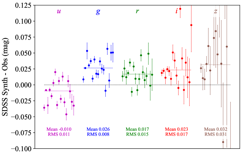
Figure 3: HST photometric residuals (in the sense of corrected observed magnitude $-$ model magnitude) for our network of DA white dwarf stars. X axis coordinates within each band are uniformly spaced, ordered by the $F275W$ magnitude with the brightest at the left. The mean and RMS are weighted by the photometric uncertainties.

The errors in this new analysis method should be smaller than the errors in the N19 method, simply because band-to-band differences effectively take out small errors in CALSPEC. This expectation is borne out, as shown in Figure 3.

5.3 Analysis Details

The first goal is limited by available computer power. Determining the posterior distribution for a model which accounts for the spectral and photometric data from all DAWDs simultaneously is judged to be impractical currently. Recognizing that the determination of $T_{\rm eff}$ and $\log~{}g$ relies almost exclusively on the spectroscopy and is nearly independent of the HST photometry, while the determination of Av and the distance modulus of each DAWD are nearly independent of the spectroscopy, we settled on a practical compromise with the following outline:

1. The analysis of N19 is performed as before for each DAWD separately. This yields for each DAWD, $s$, the posterior distribution for the apparent magnitudes in band $\lambda$, $m_{s}^{\lambda}$, and the SED parameters $T_{\rm eff}$, $\log~{}g$, and $A_{V}$

2. Using the posteriors from the previous step as input priors, the photometry of all DAWDs are incorporated simultaneously in a Bayesian model, the posteriors of which yield a second determination of the $T_{\rm eff}$, $\log~{}g$, and $A_{V}$ posteriors, together with those for the per-band zeropoint shifts $\delta_{\lambda}$ and the F160W CRNL slope, $\alpha_{CRNL}$.

If necessary for convergence, the two steps of this calculation could be iterated, incorporating the zeropoint shifts and CRNL slope from step 2 as priors into step 1. We have determined that this iteration is not necessary, a conclusion which supports the assumption of very weak coupling between the modeling of the spectroscopy and the photometry.

The calculation proceeds as follows

1. For each DAWD, a 2D normal distribution is fit to the output $T_{\rm eff}$, $\log~{}g$ chain from the N19 analysis (preceding section). These are used as priors.

2. Noninformative priors are used for $A_{V}$, with the exception of those for the primary CALSPEC DAWDs. The $A_{V}$ values of the three primary standards are constrained with an upper limit of 0.003, consistent with CALSPEC upper limits (Bohlin et al., 2020). This is a crucial element of the calculation and is the only way that the CALSPEC DAWDs play a special role.

3. The likelihood function is constructed, utilizing the same synthetic spectral model grid employed in N19.

4. A set of MCMC chains is run using emcee (Foreman-Mackey et al. 2013).

5. The posterior distributions are constructed for the output chains for the per-object $T_{\rm eff}$, $\log~{}g$, $A_{V}$, the overall model per-band zeropoint shifts, $\Delta_{\lambda}$, and the F160W CRNL slope, $\alpha_{CRNL}$.

6. As a consistency check, the $T_{\rm eff}$, $\log~{}g$, and $A_{V}$ posteriors are compared with those from the separate N19 DAWD analysis performed above. Major differences would be cause for further investigation, but in practice have not been found.

5.3.1 Likelihood function

The likelihood function for each DAWD is a small modification of that employed in N19.

$$\begin{split}P(\{m_{s}\}&|\,T_{\rm eff},\log g,A_{V},R_{V},\mu_{s},\Delta_{\lambda})=\\ &\prod_{\lambda=1}^{N_{\text{PB}}}\,N(m_{s,\lambda}|\,M_{s,\lambda}(T_{\rm eff},\log g,A_{V},R_{V})+\mu_{s}+\Delta_{\lambda},\sigma_{s,\lambda})\\ \end{split}$$ (2)

where $m_{s,\lambda}$ is the observed magnitude for a DAWD star $s$ in HST/WFC3 passband $\lambda\in\{$F275W, F336W, F475W, F625W, F775W, F160W$\}$, with photometric measurement error described by an estimated standard deviation $\sigma_{s\lambda}$, $M_{s,\lambda}(T_{\rm eff},\log g,A_{V},R_{V})$ is the synthetic magnitude of the reddened SED through passband $\lambda$, and $N(m,\sigma)$ is the normal distribution. $\mu_{s}$ is a per-star achromatic normalization parameter which is added to the synthetic reddened magnitudes in all passbands to account for the distance and radius of the DAWD $s$. $\Delta_{\lambda}$ was introduced in N16 and is the star independent offset to the observed magnitudes in passband $\lambda$ to convert them to AB magnitudes (the magnitude system for the synthetic magnitudes). If the $\Delta_{\lambda}$ were left unconstrained, there would be a degeneracy between their mean value and the mean value of the $\mu_{s}$ over the full set of stars. To break the degeneracy, we require

$$\sum_{\lambda=1}^{N_{\text{PB}}}\,\Delta_{\lambda}=0$$ (3)

The observed magnitudes for this analysis are already on the CALSPEC AB system, and the $\Delta_{\lambda}$ are expected to be quite small, accounting only for small errors in the measured HST passbands and/or aperture corrections, an expectation that is realized, as shown in Table 4. However, this constraint is not the only possible choice for breaking the degeneracy. One could, for example, instead require that the synthetic SED of a selected calibration star at a given wavelength match a value determined outside the system (e.g., CALSPEC).

Table 4: Values for $\Delta_{\lambda}$ and Their Uncertainties

Band	$\Delta$	$\Delta_{\sigma}$
	mag	mag
F275W	$-$0.004	0.001
F336W	$-$0.002	0.001
F475W	$-$0.001	0.000
F625W	$-$0.001	0.001
F775W	$-$0.000	0.001
F160W	$-$0.004	0.001

The likelihood function for the entire model is then the product over all DAWDs of the likelihood for each individual DAWD. For the results reported here, $R_{V}=3.1$.

There is one further refinement beyond the previous analysis. The HST detector for the F160W band is known to have a dependence of the counts from a source integrated over the exposure time on the rate of those counts, commonly referred to as the “count rate nonlinearity” (CRNL) (Bohlin & Deustua, 2019; Riess et al., 2019). To account for this effect, a synthetic magnitude in F160W $M_{s,F160W}$, is observed as

$$M_{s,F160W}+\alpha_{CRNL}(M_{s,F160W}-\beta_{CRNL})$$ (4)

We include $\alpha_{CRNL}$ in the free parameters of the model. We have found no significant effects from varying $\beta_{CRNL}$, and it is arbitrarily fixed at 15. The $\lambda=F160W$ term in the product in Equation 2 then becomes:

$$\begin{split}N(m_{s,F160W}|&(M_{s,F160W}+\\ &\alpha_{CRNL}(M_{s,F160W}-\beta_{CRNL})+\Delta_{F160W}+\mu_{s},\sigma_{s,F160W}))\\ \end{split}$$ (5)

It is convenient to express equation 2 as

$$\begin{split}P(\{m_{s}\}&|\,T_{\rm eff},\log g,A_{V},R_{V},\mu_{s},\Delta_{\lambda})=\\ &\prod_{\lambda=1}^{N_{\text{PB}}}\,N(m_{s,\lambda}^{corr}(\Delta_{\lambda})|\,M_{s,\lambda}(T_{\rm eff},\log g,A_{V},R_{V})+\mu_{s},\sigma_{s,\lambda})\\ \end{split}$$ (6)

where the observed magnitude, corrected for the zero point shift, and in the case of F160W, the CRNL, is

$$m^{corr}_{s,\lambda}=m_{s,\lambda}-\Delta_{\lambda}+\delta_{\lambda,F160W}\alpha_{CRNL}(m_{s,F160W}-\beta_{CRNL})$$ (7)

The values of $m^{corr}_{s,\lambda}$ are given in Table 3 alongside those for $m_{s,\lambda}$. Note that it is these values which the SEDs integrated over the WFC3 passbands are expected to match.

The free model parameters, then, include $T_{\rm eff}$, $\log~{}g$, $A_{V}$, and $\mu_{s}$ for each star, the five element array $\Delta_{\lambda}$, and $\alpha_{CRNL}$, a total of 146.

6 Results

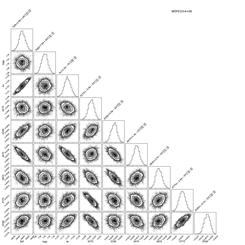
Figure 10: Corner plot showing the posterior distribution of the model parameters for WDFS1514+00. $\delta 275$ etc are the residuals as in Table 3. Note the scales.

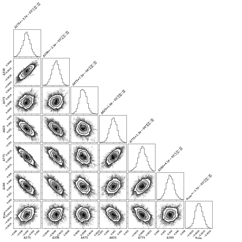
Figure 11: Corner plot showing the posterior distribution of the model parameters for $\Delta_{\lambda}$ and $\alpha_{CRNL}$. Note the scales.

We used the emcee implementation of MCMC to sample the posterior probability density function (pdf) of the model parameters employing 400 walkers, each producing a chain of 20000 steps after a 100 step burn-in. Corner plots of the resulting pdf show good convergence in all parameters. Two examples are shown in Figures 10 and 11. Derived parameters for each DAWD are presented in Table 5.

Table 5: Derived Object Parameters

Object	$T_{\rm eff}$(K)	$T_{\rm eff}$$\sigma$ (K)	$\log~{}g$ (dex)	$\log~{}g$ $\sigma$ (dex)	$A_{V}$ (mag)	$A_{V}$ $\sigma$ (mag)
G191B2B	63200	447	7.588	0.032	0.001	0.001
GD153	38765	185	7.720	0.036	0.001	0.001
GD71	32705	90	7.782	0.020	0.003	0.001
WDFS0103-00	57959	2366	7.678	0.081	0.119	0.008
WDFS0122-30	33964	215	7.771	0.031	0.048	0.005
WDFS0228-08	23026	269	7.831	0.041	0.156	0.014
WDFS0238-36	23169	84	7.880	0.014	0.171	0.005
WDFS0248+33	33148	393	7.103	0.043	0.305	0.007
WDFS0458-56	30111	78	7.788	0.018	0.014	0.003
WDFS0541-19	20436	83	7.829	0.014	0.053	0.006
WDFS0639-57	54760	890	7.898	0.048	0.162	0.004
WDFS0727+32	53516	1364	7.697	0.064	0.167	0.005
WDFS0815+07	35008	758	7.297	0.049	0.076	0.012
WDFS0956-38	19219	63	7.875	0.012	0.078	0.005
WDFS1024-00	36021	959	7.654	0.125	0.240	0.015
WDFS1055-36	29503	103	7.930	0.025	0.106	0.005
WDFS1110-17	46442	1014	8.011	0.080	0.159	0.005
WDFS1111+39	56874	1226	7.799	0.041	0.022	0.005
WDFS1206+02	23647	203	7.886	0.021	0.056	0.011
WDFS1206-27	33884	169	7.901	0.033	0.111	0.004
WDFS1214+45	34169	255	7.846	0.038	0.022	0.005
WDFS1302+10	41577	634	7.927	0.017	0.080	0.005
WDFS1314-03	43200	1397	7.823	0.091	0.110	0.010
WDFS1434-28	20332	86	7.818	0.016	0.177	0.005
WDFS1514+00	28576	127	7.903	0.013	0.120	0.005
WDFS1535-77	50524	806	9.080	0.029	0.034	0.004
WDFS1557+55	57758	983	7.551	0.070	0.029	0.004
WDFS1638+00	58415	2133	7.749	0.108	0.210	0.008
WDFS1814+78	31048	130	7.802	0.014	0.021	0.004
WDFS1837-70	19199	63	7.869	0.012	0.094	0.005
WDFS1930-52	36263	191	7.669	0.020	0.132	0.003
WDFS2101-05	29187	239	7.766	0.026	0.145	0.009
WDFS2317-29	23120	48	7.851	0.019	0.001	0.002
WDFS2329+00	20557	196	7.957	0.030	0.129	0.011
WDFS2351+37	41208	842	7.702	0.081	0.332	0.007

6.1 Comparison with CALSPEC

Despite the input photometry being on the 2014 CALSPEC system, there are small differences between our model SEDs for the CALSPEC primary DAWDs and the 2014 CALSPEC model SEDs of Bohlin et al. (2014). The absolute flux scale reported herein and our previous (N19) paper is based on the absolute flux calibration of the WFC3 filters described in C19. These spectral energy distributions (SEDs), i.e., absolute flux in physical units, are based on models of the three primary DAWDs, G191B2B, GD153, and GD71 (Bohlin et al., 2014). However, those models were improved with new NLTE grids computed by Ivan Hubeny and Thomas Rauch (Bohlin et al., 2020), which resulted in changes to the basis of the HST flux scale by up to  3% at some wavelengths. A future paper will report the SEDs of our DAWD standards, as adjusted to the more recent Bohlin et al. (2020) flux scale. See the Conclusion Section for more details.

6.2 Comparison with Gentile Fusillo 2021

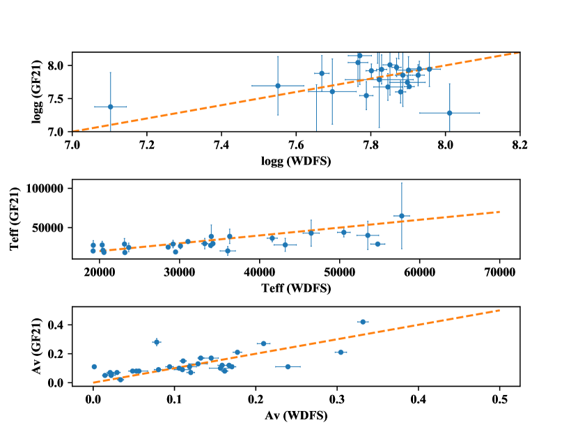
Figure 4: Comparison between our values for $\log~{}g$  $T_{\rm eff}$  and $A_{V}$  and those from Gentile Fusillo et al. (2021), denoted in the plots as GF21. The dotted lines show the identity relation. Note that a point in the $\log~{}g$  plot at approximate value 9.0 is off scale.

A new catalog of white dwarfs based on Gaia EDR3 was recently published by Gentile Fusillo et al (Gentile Fusillo et al. (2021, hereafter GF21)). This catalog contains values for the stellar parameters $T_{\rm eff}$  and $\log~{}g$  based on WD model atmospheres in conjunction with Gaia photometry, and $A_{V}$  from a three dimensional extinction model. It is useful to compare the GF21 values for our WDFS stars with our results. These are shown in Figure4. The comparison for $A_{V}$  is particularly useful, showing good agreement between values determined by two completely independent methods. The $T_{\rm eff}$  and $\log~{}g$  comparisons are likewise based on independent methods, but the a priori confidence in the GF21 values must be lowered by the lack of spectroscopic input.

6.3 Count Rate Nonlinearity

The value determined for $\alpha_{CRNL}$ is $-1.74\pm 0.32$ mmag per mag. This is significantly less than the published value of $-3.12\pm 0.32$ mmag/mag in Bohlin & Deustua (2019), or the combined result of $-3.0\pm 0.24$ mmag/mag in Riess et al. (2019). However, the CRNL is consistent with the value of $-2.36\pm 0.48$ mmag/mag for the subset of our stars analyzed in Riess et al. (2019). As shown in Figure 11, the posterior distribution for $\alpha_{CRNL}$ is tightly constrained.

6.4 Synthetic Magnitudes for Common Survey Passbands

As in N19, we have calculated the synthetic magnitudes for our standards in a number of common survey passbands. The filter passbands are obtained from the Spanish Virtual Observatory (SVO) Filter Profile Service (Rodrigo & Solano, 2020; Rodrigo et al., 2012). To calculate the synthetic magnitudes, we utilize the full MCMC chains from our analysis run, and for each point on the chain calculate the associated synthetic magnitudes. This gives a probability density function for each magnitude, which we characterized by its median and standard deviation. The standard deviations are typically less than one milli-mag (0.001 mag), significantly less in most cases than the survey reported observational uncertainties, and certainly less than the (unknown) systematic errors. The standard deviations therefore do not reflect the real uncertainties in our synthetic magnitudes, particularly in passbands not closely aligned to the HST passbands, and we do not include these values in the tables below.

For each survey system, we include below a table of our synthetic magnitudes, and where available the magnitudes and uncertainties reported by the survey. A plot for each band of each photometric system shows the magnitude differences (in the sense synthetic - observed) as a function of magnitude. We note some caveats. The observed magnitudes for each star are derived from differing photometric systems, especially the broad Gaia $G$ filter. That these independent photometric systems demonstrate good agreement between their observed and our synthetic magnitudes is further evidence for the robustness of our system.

We provide magnitudes for our stars in the DES, DECaLS, PaNSTARRS1, SDSS, and Gaia systems.

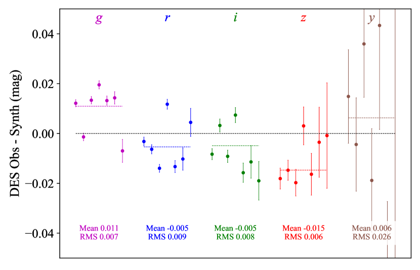
Figure 5: DES observed minus synthetic magnitudes in $grizy$. X-axis coordinates within each band are uniformly spaced, ordered by the $g$ magnitude with the brightest at the left. The mean and RMS are weighted by the photometric uncertainties. The black dashed line indicates zero difference. The mean value for each filter is represented by a dashed line through those filter’s points in the same color. Note that some points are off scale for this figure. See Table 6.

DES observed point-spread-function (PSF) magnitudes (WAVG_MAG_PSF) are from DES DR2 (Abbott et al., 2021). Results are in Table 6, and in Figure 5.

Table 6: Observed and Synthetic Photometry in DECam Bands. Units are AB mag.

Object	$u$	$u$	$g$	$g$	$r$	$r$	$i$	$i$	$z$	$z$	$y$	$y$
	Obs.	Synth.	Obs.	Synth.	Obs.	Synth.	Obs.	Synth.	Obs.	Synth.	Obs.	Synth.
G191B2B		11.114		11.502		12.092		12.491		12.820		12.982
GD153		12.772		13.096		13.655		14.044		14.368		14.528
GD71		12.526		12.797		13.335		13.715		14.035		14.192
WDFS0103-00		18.737	19.107 (2)	19.088	19.632 (3)	19.624	20.003 (4)	19.997	20.307 (11)	20.309	20.413 (48)	20.464
WDFS0122-30		18.185	18.471 (1)	18.458	18.978 (1)	18.982	19.346 (2)	19.355	19.661 (5)1	19.669	19.818 (24)	19.825
WDFS0228-08		19.801	19.816 (3)	19.827	20.218 (3)	20.221	20.527 (6)	20.531	20.816 (14)	20.802	20.997 (73)	20.936
WDFS0238-36		18.069	18.091 (1)	18.095	18.481 (1)	18.485	18.794 (2)	18.792	19.043 (3)1	19.063	19.219 (12)	19.196
WDFS0248+33		18.179		18.370		18.792		19.110		19.385		19.523
WDFS0458-56		17.530	17.770 (1)	17.754	18.272 (1)	18.273	18.637 (2)	18.645	18.939 (3)1	18.959	19.134 (15)	19.113
WDFS0541-19		18.296	18.280 (1)	18.272	18.684 (1)	18.677	18.995 (2)	18.994	19.261 (4)1	19.271	19.410 (15)	19.404
WDFS0639-57		17.841		18.177		18.692		19.054		19.360		19.512
WDFS0727+32		17.667		17.999		18.511		18.872		19.176		19.328
WDFS0815+07		19.449		19.721		20.242		20.611		20.921		21.075
WDFS0956-38		17.922		17.851		18.228		18.532		18.799		18.928
WDFS1024-00		18.669		18.911		19.365		19.700		19.989		20.133
WDFS1055-36		17.817		18.008		18.483		18.833		19.133		19.281
WDFS1110-17		17.544		17.861		18.368		18.727		19.032		19.184
WDFS1111+39		18.046		18.420		18.995		19.389		19.715		19.875
WDFS1206+02		18.604		18.673		19.114		19.448		19.737		19.878
WDFS1206-27		16.218		16.476		16.973		17.332		17.638		17.789
WDFS1214+45		17.475		17.759		18.294		18.672		18.990		19.147
WDFS1302+10		16.719		17.039		17.570		17.944		18.258		18.414
WDFS1314-03		18.782		19.100		19.622		19.991		20.302		20.456
WDFS1434-28		18.032		17.973		18.328		18.617		18.875		19.001
WDFS1514+00		15.539		15.707		16.169		16.512		16.808		16.954
WDFS1535-77		16.183		16.553		17.112		17.498		17.823		17.984
WDFS1557+55		17.098		17.470		18.044		18.436		18.761		18.921
WDFS1638+00		18.507		18.837		19.336		19.688		19.988		20.138
WDFS1814+78		16.303		16.542		17.063		17.436		17.750		17.905
WDFS1837-70		17.848		17.771		18.142		18.442		18.708		18.836
WDFS1930-52		17.210		17.482		17.981		18.339		18.643		18.794
WDFS2101-05		18.484		18.655		19.114		19.455		19.748		19.893
WDFS2317-29		18.276		18.345		18.802		19.145		19.440		19.582
WDFS2329+00		18.182	18.164 (1)	18.145	18.520 (1)	18.519	18.823 (2)	18.819	19.075 (4)1	19.087	19.247 (15)	19.217
WDFS2351+37		17.822		18.074		18.502		18.822		19.100		19.241

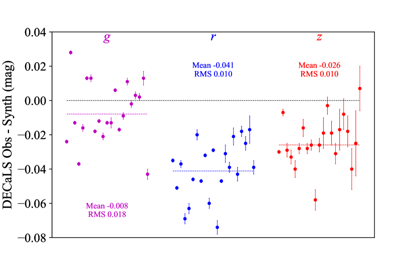
Figure 6: DECaLS Survey observed minus synthetic magnitudes in $grz$. X-axis coordinates within each band are uniformly spaced, ordered by the $g$ magnitude with the brightest at the left. The mean and RMS are weighted by the photometric uncertainties. The black dashed line indicates zero difference. The mean value for each filter is represented by a dashed line through those filter’s points in the same color. See Table 7.

DECaLS observed magnitudes are from DECaLS DR9 (Schlegel et al., 2021). Uncertainties are estimated as $2.5/\lg{10}/\texttt{snr}$. Results are in Table 7, and in Figure 6.

Table 7: Observed and Synthetic Photometry in $grz$ DECaLS Survey Bands. Units are AB mag.

Object	$g$	$g$	$r$	$r$	$z$	$z$
	Obs.	Synth.	Obs.	Synth.	Obs.	Synth.
G191B2B		11.502		12.092		12.820
GD153		13.096		13.655		14.368
GD71		12.797		13.335		14.035
WDFS0103-00	19.091 (2)	19.088	19.606 (3)	19.624	20.291 (9)1	20.309
WDFS0122-30	18.464 (1)	18.458	18.935 (1)	18.982	19.666 (5)1	19.669
WDFS0228-08	19.784 (3)	19.827	20.182 (4)	20.221	20.809 (13)	20.802
WDFS0238-36	18.077 (1)	18.095	18.438 (1)	18.485	19.035 (3)1	19.063
WDFS0248+33		18.370		18.792		19.385
WDFS0458-56	17.767 (1)	17.754	18.227 (1)	18.273	18.931 (3)1	18.959
WDFS0541-19	18.259 (1)	18.272	18.648 (1)	18.677	19.245 (4)1	19.271
WDFS0639-57	18.156 (2)	18.177	18.632 (3)	18.692	19.302 (6)1	19.360
WDFS0727+32	18.012 (2)	17.999	18.491 (3)	18.511	19.160 (5)1	19.176
WDFS0815+07	19.734 (4)	19.721	20.225 (8)	20.242	20.896 (19)	20.921
WDFS0956-38		17.851		18.228		18.799
WDFS1024-00	18.909 (2)	18.911	19.322 (4)	19.365	19.981 (9)1	19.989
WDFS1055-36		18.008		18.483		19.133
WDFS1110-17		17.861		18.368		19.032
WDFS1111+39	18.407 (3)	18.420	18.921 (4)	18.995	19.696 (9)1	19.715
WDFS1206+02	18.664 (2)	18.673	19.075 (3)	19.114	19.706 (6)1	19.737
WDFS1206-27		16.476		16.973		17.638
WDFS1214+45	17.743 (2)	17.759	18.231 (3)	18.294	18.950 (5)1	18.990
WDFS1302+10	17.026 (1)	17.039	17.533 (2)	17.570	18.229 (4)1	18.258
WDFS1314-03	19.102 (2)	19.100	19.597 (4)	19.622	20.262 (12)	20.302
WDFS1434-28		17.973		18.328		18.875
WDFS1514+00	15.683 (.4)	15.707	16.134 (.4)	16.169	16.778 (1)1	16.808
WDFS1535-77		16.553		17.112		17.823
WDFS1557+55	17.433 (1)	17.470	17.975 (3)	18.044	18.728 (4)1	18.761
WDFS1638+00	18.848 (2)	18.837	19.315 (5)	19.336	19.971 (12)	19.988
WDFS1814+78	16.570 (1)	16.542	17.012 (1)	17.063	17.743 (2)1	17.750
WDFS1837-70		17.771		18.142		18.708
WDFS1930-52		17.482		17.981		18.643
WDFS2101-05	18.638 (1)	18.655	19.083 (5)	19.114	19.729 (7)1	19.748
WDFS2317-29		18.345		18.802		19.440
WDFS2329+00	18.133 (1)	18.145	18.487 (1)	18.519	19.061 (3)1	19.087
WDFS2351+37		18.074		18.502		19.100

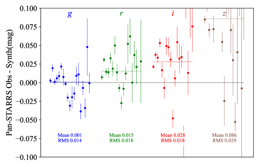
Figure 9: Pan-STARRS1 observed minus synthetic magnitudes in $griz$. X-axis coordinates within each band are uniformly spaced, ordered by the $g$ magnitude with the brightest at the left. The mean and RMS are weighted by the photometric uncertainties. The black dashed line indicates zero difference. The mean value for each filter is represented by a dashed line through those filter’s points in the same color. Note that some points are off scale for this figure. See Table 8.

PaNSTARRS1 observed PSF magnitudes are from the mean table of the DR2 (Flewelling et al., 2020). Results are in Table 8, and in Figure 9.

Table 8: Observed and Synthetic Photometry in Pan-STARRS1 $griz$ Bands. Units are AB mag.

Object	$g$	$g$	$r$	$r$	$i$	$i$	$z$	$z$
	Obs.	Synth.	Obs.	Synth.	Obs.	Synth.	Obs.	Synth.
G191B2B		11.513		11.987		12.352		12.569
GD153		13.107		13.559		13.917		14.141
GD71		12.808		13.244		13.596		13.821
WDFS0103-00	19.093 (9)1	19.100	19.570 (18)	19.533	19.979 (18)1	19.875	20.130 (69)1	20.089
WDFS0122-30		18.470		18.895		19.239		19.462
WDFS0228-08	19.837 (13)	19.837	20.188 (56)	20.159	20.523 (34)1	20.447	20.803 (88)1	20.656
WDFS0238-36		18.106		18.423		18.709		18.917
WDFS0248+33	18.351 (7)1	18.382	18.699 (8)1	18.726	18.972 (12)1	19.020	19.198 (33)1	19.223
WDFS0458-56		17.766		18.187		18.531		18.757
WDFS0541-19		18.282		18.614		18.911		19.126
WDFS0639-57		18.189		18.605		18.938		19.150
WDFS0727+32	18.018 (11)	18.011	18.475 (12)	18.425	18.806 (11)1	18.757	19.127 (30)1	18.969
WDFS0815+07	19.781 (38)	19.733	20.328 (42)	20.156	20.625 (67)1	20.497	20.710 (165)	20.718
WDFS0956-38		17.861		18.169		18.453		18.663
WDFS1024-00	18.885 (10)	18.923	19.292 (26)	19.292	19.440 (102)	19.601	19.758 (26)1	19.810
WDFS1055-36		18.019		18.405		18.730		18.949
WDFS1110-17	17.895 (4)1	17.874	18.302 (10)	18.283	18.607 (13)1	18.614	18.957 (20)1	18.828
WDFS1111+39	18.412 (14)	18.431	18.886 (8)1	18.895	19.260 (11)1	19.254	19.586 (25)1	19.473
WDFS1206+02	18.693 (12)	18.684	19.096 (26)	19.044	19.388 (19)1	19.356	19.645 (31)1	19.574
WDFS1206-27		16.488		16.891		17.223		17.441
WDFS1214+45	17.779 (6)1	17.770	18.236 (7)1	18.203	18.569 (10)1	18.553	18.849 (18)1	18.777
WDFS1302+10	17.052 (4)1	17.051	17.494 (5)1	17.480	17.858 (6)11	17.824	18.114 (9)11	18.043
WDFS1314-03	19.078 (13)	19.112	19.556 (23)	19.535	19.887 (29)1	19.874	20.240 (60)1	20.091
WDFS1434-28		17.983		18.272		18.542		18.744
WDFS1514+00	15.720 (3)1	15.718	16.101 (4)1	16.094	16.434 (2)11	16.412	16.715 (5)11	16.630
WDFS1535-77		16.565		17.013		17.367		17.587
WDFS1557+55	17.487 (5)1	17.482	17.958 (6)1	17.944	18.356 (5)11	18.303	18.647 (13)1	18.520
WDFS1638+00	18.860 (15)	18.849	19.314 (23)	19.252	19.611 (14)1	19.577	19.816 (48)1	19.786
WDFS1814+78	16.573 (5)1	16.553	17.007 (3)1	16.976	17.358 (4)11	17.321	17.651 (9)11	17.546
WDFS1837-70		17.781		18.085		18.365		18.574
WDFS1930-52		17.495		17.899		18.230		18.446
WDFS2101-05	18.652 (8)1	18.667	19.052 (8)1	19.040	19.410 (20)1	19.356	19.703 (38)1	19.572
WDFS2317-29		18.356		18.729		19.050		19.273
WDFS2329+00	18.134 (5)1	18.154	18.452 (5)1	18.460	18.772 (10)1	18.741	19.003 (13)1	18.948
WDFS2351+37	18.085 (3)1	18.086	18.447 (11)	18.434	18.776 (12)1	18.729	19.100 (38)1	18.930

The observed SDSS data for the CALSPEC DAWD standards are from Holberg & Bergeron (2006), modified to correct a typographical error in the $i$-band flux of GD153 (Holberg, private communication). The observed magnitudes for the fainter DAWDs come from SDSS DR7 (Abazajian et al. (2009)).

Table 9: Observed and Synthetic Photometry in SDSS $ugriz$ Bands. Units are AB mag.

Object	$u$	$u$	$g$	$g$	$r$	$r$	$i$	$i$	$z$	$z$
	Obs.	Synth.	Obs.	Synth.	Obs.	Synth.	Obs.	Synth.	Obs.	Synth.
G191B2B	11.033 (16)	10.997	11.470 (4)1	11.479	12.007 (7)1	12.020	12.388 (4)1	12.407	12.740 (6)11	12.766
GD153	12.700 (40)	12.667	13.022 (12)	13.075	13.573 (11)	13.585	13.950 (9)1	13.961	14.307 (16)1	14.315
GD71	12.438 (17)	12.430	12.752 (1)1	12.778	13.241 (12)	13.266	13.611 (4)1	13.633	13.973 (18)1	13.984
WDFS0103-00	18.643 (22)	18.633	19.060 (11)	19.067	19.509 (17)	19.558	19.906 (32)	19.918	20.198 (158)	20.258
WDFS0122-30		18.091		18.440		18.916		19.275		19.619
WDFS0228-08	19.798 (41)	19.765	19.769 (15)	19.820	20.150 (25)	20.166	20.367 (42)	20.461	21.197 (410)	20.760
WDFS0238-36		18.033		18.089		18.430		18.723		19.020
WDFS0248+33	18.105 (14)	18.118	18.330 (7)1	18.356	18.690 (9)1	18.736	18.921 (14)	19.040	19.213 (53)1	19.341
WDFS0458-56		17.441		17.738		18.206		18.564		18.909
WDFS0541-19		18.271		18.265		18.620		18.923		19.228
WDFS0639-57		17.742		18.157		18.627		18.977		19.310
WDFS0727+32	17.564 (11)	17.570	17.962 (6)1	17.979	18.455 (8)1	18.447	18.780 (13)	18.795	19.042 (57)1	19.126
WDFS0815+07	19.385 (28)	19.358	19.651 (12)	19.701	20.177 (23)	20.176	20.528 (37)	20.532	20.540 (153)	20.872
WDFS0956-38		17.910		17.847		18.174		18.462		18.758
WDFS1024-00	18.586 (17)	18.592	18.839 (9)1	18.896	19.292 (13)	19.306	19.592 (21)	19.627	19.759 (79)1	19.942
WDFS1055-36		17.739		17.994		18.421		18.756		19.085
WDFS1110-17	17.480 (11)	17.448	17.825 (6)1	17.843	18.294 (8)1	18.304	18.612 (12)	18.650	18.909 (43)1	18.983
WDFS1111+39	17.960 (13)	17.933	18.374 (7)1	18.398	18.905 (10)	18.925	19.264 (17)	19.305	19.628 (68)1	19.661
WDFS1206+02		18.553		18.663		19.054		19.374		19.692
WDFS1206-27		16.130		16.459		16.909		17.254		17.588
WDFS1214+45	17.358 (9)1	17.378	17.700 (5)1	17.740	18.197 (7)1	18.226	18.540 (12)	18.591	18.763 (34)1	18.939
WDFS1302+10	16.637 (8)1	16.619	16.982 (4)1	17.019	17.468 (6)1	17.503	17.842 (7)1	17.864	18.146 (28)1	18.207
WDFS1314-03		18.684		19.081		19.557		19.912		20.251
WDFS1434-28		18.021		17.969		18.276		18.551		18.836
WDFS1514+00	15.475 (4)1	15.467	15.663 (3)1	15.694	16.089 (4)1	16.108	16.412 (4)1	16.437	16.728 (12)1	16.761
WDFS1535-77		16.073		16.533		17.042		17.415		17.770
WDFS1557+55	16.982 (8)1	16.985	17.438 (5)1	17.448	17.985 (7)1	17.974	18.344 (10)	18.353	18.685 (38)1	18.708
WDFS1638+00		18.412		18.817		19.273		19.613		19.939
WDFS1814+78		16.213		16.525		16.996		17.355		17.700
WDFS1837-70		17.838		17.768		18.088		18.374		18.667
WDFS1930-52		17.121		17.464		17.917		18.262		18.594
WDFS2101-05	18.460 (17)	18.414	18.651 (9)1	18.642	19.046 (12)	19.053	19.388 (22)	19.380	19.791 (93)1	19.701
WDFS2317-29		18.223		18.334		18.740		19.069		19.394
WDFS2329+00		18.161		18.140		18.465		18.751		19.045
WDFS2351+37	17.771 (11)	17.749	18.022 (6)1	18.059	18.437 (8)1	18.446	18.757 (11)	18.752	19.007 (46)1	19.055

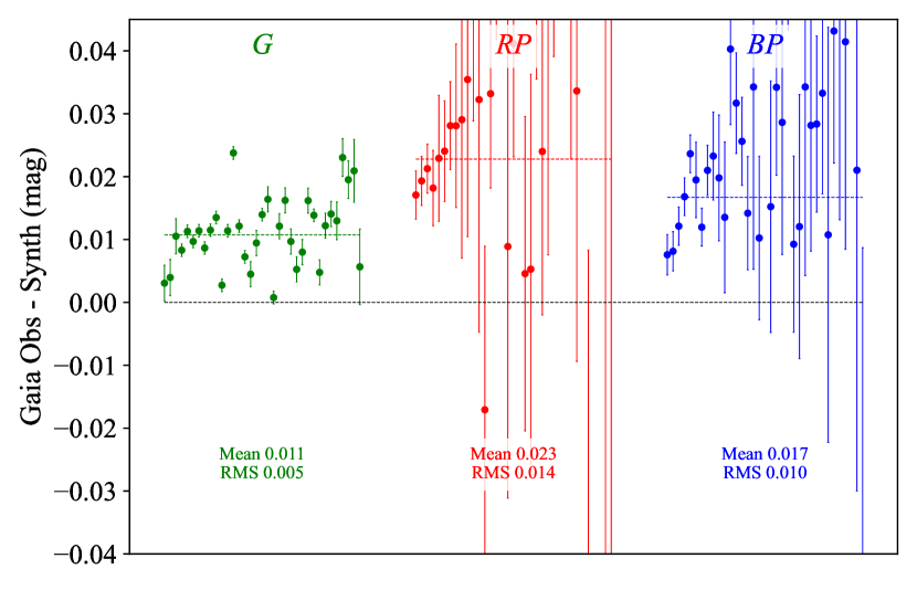
Figure 7: Gaia DES observed minus synthetic magnitudes in $G$, $RP$, and $BP$. X-axis coordinates within each band are uniformly spaced, ordered by the $G$ magnitude with the brightest at the left. The mean and RMS are weighted by the photometric uncertainties. The black dashed line indicates zero difference. The mean value for each filter is represented by a dashed line through those filter’s points in the same color. See Table 10.

Gaia observed magnitudes are from DR3 (Gaia Collaboration et al., 2022). For comparison to DR3 magnitudes, our synthetic magnitudes are transformed from AB to Vega using passband data from Rodrigo & Solano (2020). Results are in Table 10, and Figure 7.

Table 10: Observed and Synthetic Photometry in Gaia Bands. Units are Vega mag.

Object	$G$	$G$	$RP$	$RP$	$BP$	$BP$
	Obs.	Synth.	Obs.	Synth.	Obs.	Synth.
G191B2B	11.718 (3)	11.715	12.071 (4)11	12.054	11.546 (3)1	11.539
GD153	13.311 (3)	13.300	13.632 (4)11	13.611	13.151 (3)1	13.139
GD71	13.000 (3)	12.996	13.305 (4)11	13.286	12.853 (3)1	12.845
WDFS0103-00	19.302 (3)	19.279	19.672 (53)1	19.566	19.164 (33)	19.123
WDFS0122-30	18.664 (1)	18.650	19.010 (32)1	18.927	18.532 (14)	18.504
WDFS0228-08	19.975 (6)	19.969	20.068 (171)	20.120	19.820 (75)	19.886
WDFS0238-36	18.236 (1)	18.235	18.386 (25)1	18.381	18.188 (14)	18.154
WDFS0248+33	18.521 (2)	18.516	18.742 (43)1	18.691	18.423 (21)	18.411
WDFS0458-56	17.959 (1)	17.948	18.251 (37)1	18.219	17.847 (12)	17.807
WDFS0541-19	18.433 (2)	18.423	18.607 (26)1	18.583	18.349 (14)	18.340
WDFS0639-57	18.375 (2)	18.359	18.702 (41)1	18.625	18.269 (15)	18.211
WDFS0727+32	18.189 (2)	18.180	18.452 (40)1	18.443	18.043 (13)	18.033
WDFS0815+07	19.932 (5)	19.911	20.248 (129)	20.183	19.787 (51)	19.766
WDFS0956-38	18.002 (1)	17.990	18.157 (15)1	18.124	17.945 (7)1	17.919
WDFS1024-00	19.083 (3)	19.070	19.234 (53)1	19.279	18.996 (33)	18.950
WDFS1055-36	18.196 (1)	18.182	18.453 (18)1	18.412	18.121 (11)	18.058
WDFS1110-17	18.048 (1)	18.041	18.372 (30)1	18.300	17.911 (9)1	17.897
WDFS1111+39	18.644 (2)	18.628	19.067 (53)1	18.953	18.485 (20)	18.457
WDFS1206+02	18.850 (2)	18.838	19.066 (43)1	19.032	18.746 (33)	18.735
WDFS1206-27	16.667 (1)	16.656	16.930 (10)1	16.907	16.543 (3)1	16.519
WDFS1214+45	17.979 (1)	17.955	18.226 (26)1	18.243	17.836 (8)1	17.804
WDFS1302+10	17.239 (1)	17.230	17.542 (13)1	17.514	17.099 (4)1	17.078
WDFS1314-03	19.307 (3)	19.287	19.745 (83)1	19.562	19.252 (31)	19.138
WDFS1434-28	18.103 (2)	18.099	18.352 (30)1	18.211	18.070 (29)	18.036
WDFS1514+00	15.884 (1)	15.876	16.111 (6)11	16.093	15.775 (3)1	15.758
WDFS1535-77	16.765 (1)	16.754	17.095 (7)11	17.067	16.600 (3)1	16.588
WDFS1557+55	17.691 (1)	17.678	18.036 (25)1	18.001	17.527 (10)	17.507
WDFS1638+00	19.025 (2)	19.011	19.362 (41)1	19.261	18.912 (21)	18.869
WDFS1814+78	16.745 (1)	16.735	17.033 (8)11	17.009	16.612 (6)1	16.593
WDFS1837-70	17.910 (1)	17.907	18.081 (17)1	18.035	17.853 (12)	17.839
WDFS1930-52	17.673 (1)	17.662	17.942 (22)1	17.913	17.547 (7)1	17.524
WDFS2101-05	18.827 (2)	18.822	19.096 (38)1	19.035	18.739 (16)	18.706
WDFS2317-29	18.526 (2)	18.518	18.809 (42)1	18.728	18.444 (30)	18.410
WDFS2329+00	18.292 (2)	18.280	18.417 (31)1	18.412	18.237 (21)	18.208
WDFS2351+37	18.235 (2)	18.219	18.500 (26)1	18.403	18.122 (20)	18.107

Our synthetic magnitudes are anchored on observations made above the atmosphere. With the exception of Gaia, all other surveys in this comparison are from ground- based surveys, which have required accounting for the constantly changing extinction from the terrestrial atmosphere. We hope that the network of spectrophotometric standard stars presented in this paper will be a useful tool for resolving any discrepancies between different surveys. Beyond this, we have not attempted to ascribe specific causes for the discrepancies between our synthetic magnitudes for these surveys and those published by the surveys themselves. To do so would require significant expertise from the survey teams, and could form a focus for future work. Similarly, the impact of any downstream scientific results from any re-calibration of existing surveys is best left to the discretion of topical experts, and the specific problems they have at hand.

7 Conclusions

7.1 Major results of this paper

This and prior papers (N19, C19, and C22) work towards an all-sky network of faint spectrophotometric standard stars (called WDFS) composed of hot DAWDs whose fluxes are tied to the three primary CALSPEC standards. Our initial goal of 1% absolute and 0.5% relative flux calibration in the visual band is realized and our network of 35 White Dwarf Flux Standards (32 WDFS and 3 CALSPEC) is available for general use. In addition, each stellar reddened SED provides predicted magnitudes in several common survey systems (6.4). This set of stars covers the entire sky, such that, at any time, two or more standards are above 2 airmasses, at any ground-based observatory. Because the HST/WFC3 photometry that defines our system is above the atmosphere, ground-based, atmospheric extinction problems do not exist. Our standards are suitable for many of the existing and future large telescope surveys.

The conversion of our derived SEDs to magnitudes in ground based surveys must necessarily include the filter functions of the surveys, which are often available (Rodrigo & Solano, 2020; Rodrigo et al., 2012). Our published SEDs can be convolved with any filter function for any telescope. If these functions are not known, a later paper in this series, using parallel ACS images, can define color terms for conversion of native ground-based magnitudes to magnitudes on the space-based system.

Item 4 of the next section discusses extrapolations of our SEDs shortward of the HST F275W passband and longward of the infrared F160W passband.

7.2 Possible Improvements and Enhancements

The following items discuss some limitations of this sample and some possible future improvements.

1. By their very nature, our white dwarf stars have blue SEDs. If our standards are used for the calibration of broadband photometry for much redder stars, the extreme color of our WDFS stars could be problematic. In this regard, our ACS fields (in prep) will provide photometry from the ACS/HST fields that were observed in parallel with the WFC3 observations. These fields include approximately 100-200 stars of different spectral types within 4-6 arcminutes of our WDFS stars and should be helpful in photometrically linking our blue standards DAWDs with redder stars.

2. Our absolute photometry is tied to CALSPEC, which has an estimated uncertainty of 1% and is ultimately linked to the monochromatic flux of Vega at 5556 Å and Sirius in the IR (Bohlin, 2014; Bohlin et al., 2020), which have their own uncertainties. Ongoing and proposed ground-based and space-based efforts seek to establish stellar calibrations with respect to NIST (National Institute of Standards and Technology) laboratory radiometry with 0.5% absolute and 0.3% relative uncertainties in the visual. When available, these improvements can be applied to our existing WDFS by making global corrections at the few tenths of a percent level.

3. Future expansion of our standard star network is possible. The size of our network was ultimately dictated by the observational effort required to locate and validate suitable candidates, as well as monitoring each star for photometric stability, by obtaining the spectroscopic time on large telescopes, and by obtaining the WFC3 photometry in six bands. Future efforts can rely on current deep multifiber spectroscopic surveys to identify large numbers of suitable candidate DAWD standards. Likewise, multi-epoch photometry from Gaia and RST can verify photometric stability of these candidates. However, our unique step that uses WFC3 photometry will be impossible after HST is decommissioned.

4. Extensions of wavelength range. Our fluxes are well defined over the wavelength range 2750 Å to 1.6$\mu m$ by WFC3 photometry. In order to validate our treatment of interstellar extinction and our model fluxes below 2750 Å, a new STIS/HST program obtained observations of about two thirds of our WDFS stars in the UV down to 1150 Å. Preliminary results from this program show that our optically estimated values of $A_{V}$ predict the observed UV fluxes for most stars to a precision better than 3%. Outliers might be explained by adjusting $A_{V}$ and $R_{V}$, the ratio of absolute extinction $A_{V}$ to selective extinction E(B-V), within our uncertainties. There are no observational tests longward of the F160W passband, but there is exquisite agreement between models and observations at shorter wavelengths.

5. The placement of our WDFS SEDs on the CALSPEC absolute flux scale has several inaccuracies at the percent level that will be addressed in our next paper. First, our model SEDs are in air above 2000 Å. The air to vacuum correction that is applied to our final SEDs is adequate, except for a small unphysical discontinuity at 2000 Å, but these models extend to only 1350 Å in the FUV and $2.7\mu$ in the IR. CALSPEC now utilizes the NLTE grids computed by I. Hubeny and T. Rauch (Bohlin et al., 2020) that cover 900 Å to 30$\mu$ with native vacuum wavelengths and show emission lines at HI line centers where these features are actually observed. Furthermore, these newer NLTE grids include many more IR lines, including some important features like Paschen $\alpha$. Measurements of radial velocities would improve our model SEDs slightly.

   Perhaps the most important WDFS future improvement will be to place the absolute fluxes on the updated scale of Bohlin et al. (2020). Figure 12 illustrates quantitative comparisons with these old and new flux scales (GD153 is corrected for the published radial velocity of 8.3 km s^-1 Napiwotzki et al., 2020). The blue curve compares our GD153 model with the 2014 gd153_mod_010.fits and is generally within 1% of agreement, except in the line profiles and at the shortest wavelengths. Because our flux scale is based on the 2014 models and the WFC3 calibration of Calamida et al. (2019) that is used in in our previous papers, the blue trace represents the small offset between our flux scale and the 2014 CALSPEC flux system. The difference between the red and blue is the amount of change in 2020 to the gd153_mod_011.fits model of Bohlin et al. (2020).

8 Data Availability

We have created a Zenodo url that contains the SEDs derived in this paper, the WFC3 passbands we employed to create magnitudes in commonly used systems, and derived parameters for each star (Table 5 in the text), along with all of the other tables. These data and the corrected, ”c”, magnitudes in Table 2 define our magnitudes in Tables 6-10. DAWD-based magnitudes for an arbitrary system/telescope can be derived given atmospheric transmission plus filter, mirror, and CCD efficiencies.

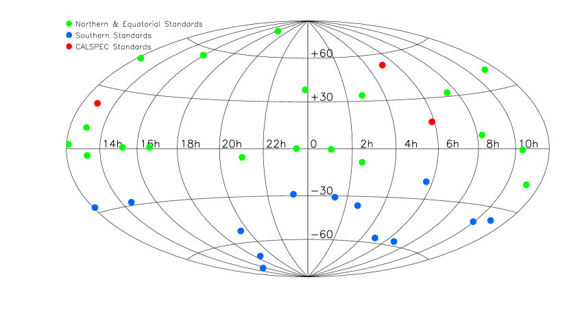
Figure 1: Aitoff projection of our network of spectrophotometric standard DAWDs illustrating the full-sky nature of our system (HST Cycles 20 and 22 in green, Cycle 25 in blue, and the three bright CALSPEC DAWDs in red).

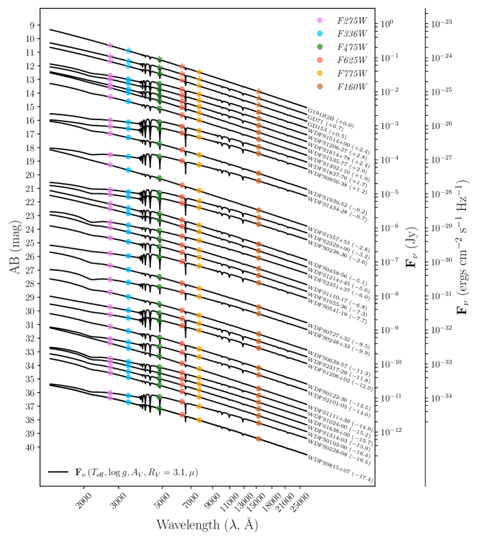
Figure 2: Calculated SEDs for all DAWDs in our network with synthetic HST magnitudes overlaid (colored points). Each spectrum is arbitrarily shifted in AB mag for clarity.

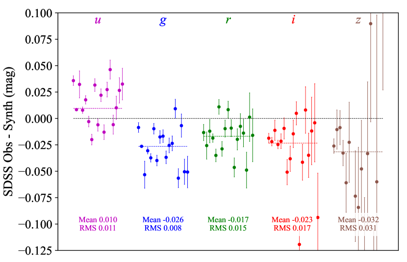
Figure 8: SDSS observed minus synthetic magnitudes in $ugrizy$. X-axis coordinates within each band are uniformly spaced, ordered by the $g$ magnitude with the brightest at the left. The mean and RMS are weighted by the photometric uncertainties. The black dashed line indicates zero difference. The mean value for each filter is represented by a dashed line through those filter’s points in the same color. Note that some points are off scale for this figure. See Table 9.

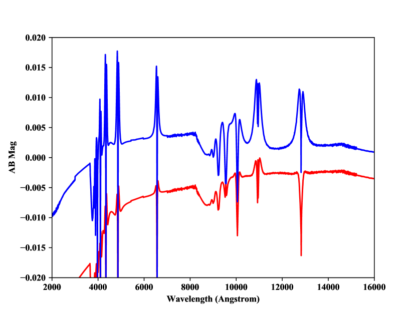
Figure 12: Comparison between our model SED for GD153 and that of two CALSPEC SEDs. The blue curve shows the AB magnitude difference between the SED for GD153 from the version of CALSPEC (gd153_mod_010.fits) in use till 2019 and that derived in this paper. The red curve shows the same difference, but for the 2020 CALSPEC. The 2020 CALSPEC SED uses newer atmosphere models than the 2019 SED, with an additional change in the calibration of the achromatic absolute magnitude zero-point making the CALSPEC 2020 fluxes brighter by 0.0087 mag.

References

- Abazajian et al. (2009) Abazajian, K. N., Adelman-McCarthy, J. K., Agüeros, M. A., et al. 2009, ApJS, 182, 543, doi: 10.1088/0067-0049/182/2/543
- Abbott et al. (2021) Abbott, T. M. C., Adamów, M., Aguena, M., et al. 2021, ApJS, 255, 20, doi: 10.3847/1538-4365/ac00b3
- Betoule et al. (2013) Betoule, M., Marriner, J., Regnault, N., et al. 2013, A&A, 552, A124, doi: 10.1051/0004-6361/201220610
- Bohlin (2014) Bohlin, R. C. 2014, The Astronomical Journal, 147, 127, doi: 10.1088/0004-6256/147/6/127
- Bohlin & Deustua (2019) Bohlin, R. C., & Deustua, S. E. 2019, AJ, 157, 229, doi: 10.3847/1538-3881/ab1b50
- Bohlin et al. (2014) Bohlin, R. C., Gordon, K. D., & Tremblay, P. E. 2014, Publications of the Astronomical Society of the Pacific, 126, 711, doi: 10.1086/677655
- Bohlin et al. (2020) Bohlin, R. C., Hubeny, I., & Rauch, T. 2020, AJ, 160, 21, doi: 10.3847/1538-3881/ab94b4
- Bohlin et al. (2022) Bohlin, R. C., Krick, J. E., Gordon, K. D., & Hubeny, I. 2022, AJ, 164, 10, doi: 10.3847/1538-3881/ac6fe1
- Calamida et al. (2019) Calamida, A., Matheson, T., Saha, A., et al. 2019, ApJ, 872, 199, doi: 10.3847/1538-4357/aafb13
- Calamida et al. (2022a) Calamida, A., Matheson, T., Olszewski, E. W., et al. 2022a, arXiv e-prints, arXiv:2209.09950. https://arxiv.org/abs/2209.09950
- Calamida et al. (2022b) Calamida, A., Bajaj, V., Mack, J., et al. 2022b, AJ, 164, 32, doi: 10.3847/1538-3881/ac73f0
- Dufour et al. (2017) Dufour, P., Blouin, S., Coutu, S., et al. 2017, in Astronomical Society of the Pacific Conference Series, Vol. 509, 20th European White Dwarf Workshop, ed. P. E. Tremblay, B. Gaensicke, & T. Marsh, 3, doi: 10.48550/arXiv.1610.00986
- Eisenstein et al. (2006) Eisenstein, D. J., Liebert, J., Harris, H. C., et al. 2006, ApJS, 167, 40, doi: 10.1086/507110
- Flewelling et al. (2020) Flewelling, H. A., Magnier, E. A., Chambers, K. C., et al. 2020, ApJS, 251, 7, doi: 10.3847/1538-4365/abb82d
- Foreman-Mackey et al. (2013) Foreman-Mackey, D., Hogg, D. W., Lang, D., & Goodman, J. 2013, PASP, 125, 306, doi: 10.1086/670067
- Fukugita et al. (1996) Fukugita, M., Ichikawa, T., Gunn, J. E., et al. 1996, AJ, 111, 1748, doi: 10.1086/117915
- Gaia Collaboration et al. (2022) Gaia Collaboration, Vallenari, A., Brown, A. G. A., et al. 2022, arXiv e-prints, arXiv:2208.00211, doi: 10.48550/arXiv.2208.00211
- Gentile Fusillo et al. (2017) Gentile Fusillo, N. P., Raddi, R., Gänsicke, B. T., et al. 2017, MNRAS, 469, 621, doi: 10.1093/mnras/stx777
- Gentile Fusillo et al. (2021) Gentile Fusillo, N. P., Tremblay, P. E., Cukanovaite, E., et al. 2021, MNRAS, 508, 3877, doi: 10.1093/mnras/stab2672
- Holberg & Bergeron (2006) Holberg, J. B., & Bergeron, P. 2006, AJ, 132, 1221, doi: 10.1086/505938
- Holberg et al. (1985) Holberg, J. B., Wesemael, F., Wegner, G., & Bruhweiler, F. C. 1985, ApJ, 293, 294, doi: 10.1086/163237
- Hubeny & Lanz (1995) Hubeny, I., & Lanz, T. 1995, ApJ, 439, 875, doi: 10.1086/175226
- Kleinman et al. (2004) Kleinman, S. J., Harris, H. C., Eisenstein, D. J., et al. 2004, ApJ, 607, 426, doi: 10.1086/383464
- Loredo & Hendry (2019) Loredo, T. J., & Hendry, M. A. 2019, arXiv e-prints, arXiv:1911.12337. https://arxiv.org/abs/1911.12337
- McCook & Sion (1999) McCook, G. P., & Sion, E. M. 1999, ApJS, 121, 1, doi: 10.1086/313186
- Megessier (1995) Megessier, C. 1995, A&A, 296, 771
- Napiwotzki et al. (2020) Napiwotzki, R., Karl, C. A., Lisker, T., et al. 2020, A&A, 638, A131, doi: 10.1051/0004-6361/201629648
- Narayan et al. (2016) Narayan, G., Axelrod, T., Holberg, J. B., et al. 2016, ApJ, 822, 67, doi: 10.3847/0004-637X/822/2/67
- Narayan et al. (2019) Narayan, G., Matheson, T., Saha, A., et al. 2019, The Astrophysical Journal Supplement Series, 241, 20, doi: 10.3847/1538-4365/ab0557
- Raddi et al. (2016) Raddi, R., Catalán, S., Gänsicke, B. T., et al. 2016, MNRAS, 457, 1988, doi: 10.1093/mnras/stw042
- Raddi et al. (2017) Raddi, R., Gentile Fusillo, N. P., Pala, A. F., et al. 2017, MNRAS, 472, 4173, doi: 10.1093/mnras/stx2243
- Riess et al. (2019) Riess, A. G., Narayan, G., & Calamida, A. 2019, Calibration of the WFC3-IR Count-rate Nonlinearity, Sub-percent Accuracy for a Factor of a Million in Flux, Instrument Science Report WFC3 2019-1, 13 pages
- Rodrigo & Solano (2020) Rodrigo, C., & Solano, E. 2020, in XIV.0 Scientific Meeting (virtual) of the Spanish Astronomical Society, 182
- Rodrigo et al. (2012) Rodrigo, C., Solano, E., & Bayo, A. 2012, SVO Filter Profile Service Version 1.0, IVOA Working Draft 15 October 2012, doi: 10.5479/ADS/bib/2012ivoa.rept.1015R
- Schlegel et al. (2021) Schlegel, D., Dey, A., Herrera, D., et al. 2021, in American Astronomical Society Meeting Abstracts, Vol. 53, American Astronomical Society Meeting Abstracts, 235.03