Distribution free MMD tests for model selection with estimated parameters

Abstract

Several kernel based testing procedures are proposed to solve the problem of model selection in the presence of parameter estimation in a family of candidate models. Extending the two sample test of Gretton et al. (2006), we first provide a way of testing whether some data is drawn from a given parametric model (model specification). Second, we provide a test statistic to decide whether two parametric models are equally valid to describe some data (model comparison), in the spirit of Vuong (1989). All our tests are asymptotically standard normal under the null, even when the true underlying distribution belongs to the competing parametric families. Some simulations illustrate the performance of our tests in terms of power and level.

1 Introduction

Model selection is an “umbrella term” that refers to different important statistical problems, with a significant influence on drawn conclusions. First, any parametric or semiparametric model has to be validated theoretically, most often by statistical tests, inducing the field of “specification testing”. In this work, we will consider models that specify the law of a Data Generating Process (DGP), i.e., we consider models of probability distributions. Thus, a model, say $\mathcal{M}$, is assimilated to a family of distributions $\mathcal{M}:=\{P_{\alpha},\alpha\in\Theta_{\alpha}\}$, where $\Theta_{\alpha}$ denotes some index set. The “true” underlying law of the DGP is denoted by $P$. The empirical law of a sample of $n$ i.i.d. observations from $P$ is denoted $\mathbb{P}_{n}$. To obtain consistent specification tests, it is necessary to measure the distance between a suggested model and the true underlying DGP. This is commonly done in terms of a semi-metric $\pi$ between probability distributions. The distance between the model $\mathcal{M}$ and the law $P$ of the DGP is then defined as

$$\pi(\mathcal{M},P):=\inf_{\alpha\in\Theta_{\alpha}}\pi(P_{\alpha},P).$$

This definition allows to conduct a hypothesis test of

$$\mathcal{H}_{0,\mathcal{M}}:\pi(\mathcal{M},P)=0,$$

which is a natural way of testing the hypothesis that the model for the DGP is correctly specified. This general framework includes all well-known tests as Chi-squared, Kolmogorov-Smirnov, Cramer-von Mises, etc. We can define the best-fitting probability distributions in the family $\mathcal{M}$ by defining so-called pseudo-true parameter(s) $\alpha_{\star}$ that minimize the distance between the model $\mathcal{M}$ and the DGP, i.e.,

$$\alpha_{\star}:=\arg\min_{\alpha\in\Theta_{\alpha}}\pi(P_{\alpha},P).$$

Clearly, such ${\alpha_{\star}}$ are unknown in practice and an estimator ${\alpha_{n}}$ of $\alpha_{\star}$ has to be used to find the optimal model in $\mathcal{M}$. Further, $P$ is often also unknown and needs to be estimated via $\mathbb{P}_{n}$. Therefore, in practical applications, a consistent test of $\mathcal{H}_{0,\mathcal{M}}$ cannot be directly conducted with an estimator of $\pi(P_{\alpha_{\star}},P)=0$, but needs to be based on the asymptotic distribution of an estimator of $\pi(P_{{\alpha_{n}}},\mathbb{P}_{n})$ under the null hypothesis.

Since the seminal works of Durbin ([18, 19, 20]), numerous consistent specification tests have been proposed in the statistical literature, depending on the chosen distance $\pi$, but only a few of them manage composite assumptions. This is the case with the Cramer-von Mises and Kolmogorov distances ([36]), the uniform distance between multivariate cdfs’ ([10, 9]), the total variation distance or, equivalently, the $L^{1}$ distance between the underlying densities ([15]), a $L^{2}$-type distance between characteristic functions ([22]), Wasserstein’s distance ([27]), Kernel Stein Discrepancies ([30]), among others. Another perspective would be to focus on models of some distributional features of $P$. For instance, regression models restrict themselves to specifying conditional moments only, not DGPs. In this case, the associated specification tests may not be based on distances between distributions, because model-DGPs are partly unspecified. They rather rely on other lack-of-fit measures, typically given by moment type conditions: see a general framework and examples in [37, 44] or, e.g., the textbook [11, Part I]. However, there are also attempts to combine the distributional- and the regression-type approaches. In the presence of covariates, [4] defined a conditional Kolmogorov test for testing general conditional distributions, by comparing the empirical distribution function of the data with the corresponding empirical distribution function implied by the model. The ICM test of [12] is based on the same idea, but working with a $L^{2}$-type distance between empirical characteristic functions. [52] compares a parametric conditional density with a corresponding non-parametric kernel estimator via an approximation of the Kullback–Leibler information criterion. In this paper, we do not consider covariates or conditional laws. Therefore, we hereafter restrict ourselves to the setting where a model specifies a family of (unconditional) probability distributions.

Second, when there exist several competing models, “model selection” rather means validating one of the competing model as “the better one”. The aim is then to identify the model(s) that is(are) the closest to the DGP, a task that is called “model comparison”. The seminal paper [49] was the first to propose a general framework for this task. The author proposed to use the Kullback-Leibler (KL) divergence for model comparison: a model $\mathcal{M}_{1}$ is preferred over a model $\mathcal{M}_{2}$ when its distance to the true model is the smallest, i.e., when $\pi(\mathcal{M}_{1},P)<\pi(\mathcal{M}_{2},P)$ where $\pi$ is chosen as the Kullback-Leibler divergence. In general, model selection between competing models is based on tests of the null hypothesis

$$\mathcal{H}_{0,\mathcal{M}_{1},\mathcal{M}_{2}}:\pi(\mathcal{M}_{1},P)=\pi(\mathcal{M}_{2},P).$$

In most circumstances, the competing models are parametric and may be misspecified, i.e., none of the models will satisfy $\pi(\mathcal{M}_{i},P)=0$, $i\in\{1,2\}$. For instance, when $\mathcal{M}_{1}=\{P_{\alpha},\alpha\in\Theta_{\alpha}\}$ and $\mathcal{M}_{2}=\{P_{\beta},\beta\in\Theta_{\beta}\}$, their pseudo-true values are defined as above by

$${\alpha_{\star}}:=\operatorname{argmin}_{\alpha\in\Theta_{\alpha}}\pi(P_{\alpha},P),\;\text{and}\;{\beta_{\star}}:=\operatorname{argmin}_{\beta\in\Theta_{\beta}}\pi(P_{\beta},P).$$ (1)

Then, $\mathcal{H}_{0,\mathcal{M}_{1},\mathcal{M}_{2}}$ may be rewritten as

$$\mathcal{H}_{0,\mathcal{M}_{1},\mathcal{M}_{2}}:\pi(P_{{\alpha_{\star}}},P)=\pi(P_{{\beta_{\star}}},P).$$

Once some estimated pseudo-true values ${\alpha_{n}}$ and ${\beta_{n}}$ and a sample from $P$ are available, a model selection test is typically based on the random quantities

$$\mathcal{T}_{n}:=\hat{\pi}(P_{\alpha_{n}},\mathbb{P}_{n})-\hat{\pi}(P_{\beta_{n}},\mathbb{P}_{n}),$$

where $\hat{\pi}(P_{1},P_{2})$ denotes an estimator of $\pi(P_{1},P_{2})$ for any couple of probability distributions $(P_{1},P_{2})$. Unfortunately, the asymptotic distribution of $\mathcal{T}_{n}$ is generally complex. Indeed, the randomness of the estimated parameters of both models matter to state the limiting law of $\mathcal{T}_{n}$ under $\mathcal{H}_{0,\mathcal{M}_{1},\mathcal{M}_{2}}$. This is particularly the case for overlapping models, i.e. for models $\mathcal{M}_{1}$ and $\mathcal{M}_{2}$ for which $P_{\alpha_{\star}}=P_{\beta_{\star}}$, a situation that often cannot be excluded. For example, this is the case for the KL divergence, where $\mathcal{T}_{n}$ is no longer distribution-free, see [49, Theorem 3.3]. Moreover, the methodology of [49] requires pre-testing to know whether the competing models are overlapping, a feature that is generally considered as a drawback. Some variations of the traditional test of [49] have been proposed in the literature to avoid pre-testing and to keep its asymptotic standard normal distribution, see notably [43, 39, 32] and the references therein.

The aim of this paper is to provide a solution for “specification testing” and “model comparison” when $\pi$ is the Maximum Mean Discrepancy (MMD). Since the latter distance has a direct and natural interpretation in terms of mean embeddings in Reproducing Kernel Hilbert Spaces, it has become very popular in machine learning and statistics since its introduction in [24, 45], see [35] for a more recent review of the topic. MMD has proven to be a robust method for inference purposes ([16, 3]), change-point detection ([8]), relative goodness-of-fit tests [13], copula estimation ([2]), GAN training ([31, 21]), among other domains. The attractive feature of MMD is that it can be used in general and/or high-dimensional spaces and that it can be simply estimated by sampling from the underlying distributions. Therefore, specification testing and model comparison procedures based on MMD retain the attractive features of being applicable to general probability spaces and simple computability in practice. Furthermore, [40] showed that every choice of $\operatorname{MMD}$ is in one-to-one correspondence to so-called generalized energy distances. Due to their simple representation as a sum of expected distances between random vectors, generalized energy distances are highly popular in applied statistics: see [14, 38, 29, 28], e.g. Note that the so-called distance correlation [47], a popular measure of dependence between random vectors, is also essentially based on energy distances. Thus, the one-to-one correspondence of generalized energy distances and $\operatorname{MMD}$s allows to directly translate the model specification and model comparison procedures proposed in this paper to model specification and model comparison in the framework of generalized energy distances.

Let us recall the basics about MMD, following the approach of [25]. Consider some probability distributions defined on some topological space $\mathcal{S}$. Instead of comparing these probability distributions directly on the space of probability measures, they may be mapped into a reproducing kernel Hilbert space of real-valued functions $\mathcal{H}$ defined on $\mathcal{S}$. The latter space is associated with a symmetric and positive definite measurable map $k:\mathcal{S}\times\mathcal{S}\to\mathbb{R}$, called kernel. For many kernels $k$ (called “characteristic”), these mappings are injective and the MMD distance between probability distributions is then defined as the distance between their respective embeddings in the space of functions $\mathcal{H}$. More specifically, consider some random elements $X$ in a measurable space $(\mathcal{S},\mathcal{A})$, whose law is $P$. The embedding of the probability measure $P$ into $\mathcal{H}$ is given by the map $P\mapsto\mathbb{E}_{P}\left[k(\cdot,X)\right]=:\mu_{P}$. The latter map implicitly depends on the kernel $k$, but this dependence is removed to lighten notations. When $k$ is characteristic, $P\mapsto\mu_{P}$ is injective and we have $P_{1}\not=P_{2}$ iff $\mu_{P_{1}}\not=\mu_{P_{2}}$. Thus, the Maximum-Mean-Discrepancy is defined as the distance on the space of probability measures on $\mathcal{S}$ via

$$\operatorname{MMD}(P_{1},P_{2}):=\sqrt{\|\mu_{P_{1}}-\mu_{P_{2}}\|_{\mathcal{H}}}.$$

Since one can show that $\langle\mu_{P},f\rangle=\mathbb{E}_{P}\left[f(X)\right]$ for all $f\in\mathcal{H}$ such that $\mathbb{E}\left[f(X)\right]$ exists, one can deduce that

$$\operatorname{MMD}^{2}(P_{1},P_{2}):=\mathbb{E}_{X,X^{\prime}\sim P_{1}}\Big{[}\mathbb{E}_{Y,Y^{\prime}\sim P_{2}}\big{[}k(X,X^{\prime})-2k(X,Y)+k(Y,Y^{\prime})\big{]}\Big{]}.$$

Therefore, the computation of $\operatorname{MMD}(P_{1},P_{2})$ does not involve any operations in the Hilbert space $\mathcal{H}$ but is solely given in terms of expectations of known functions w.r.t. to $P_{1}$ and/or $P_{2}$. Moreover, given an i.i.d. sample $(X_{1},X_{2},\ldots)$ from $P_{1}$ and $(Y_{1},Y_{2},\ldots)$ from $P_{2}$, $\operatorname{MMD}^{2}(P_{1},P_{2})$ can be empirically estimated by

$$\widehat{\operatorname{MMD}^{2}}(P_{1},P_{2}):=\frac{1}{n(n-1)}\sum_{\begin{subarray}{c}i,j=1\\ i\not=j\end{subarray}}^{n}\big{\{}k(X_{i},X_{j})-2k(X_{i},Y_{j})+k(Y_{i},Y_{j})\big{\}}.$$ (2)

The latter unbiased estimator of $\operatorname{MMD}^{2}(P_{1},P_{2})$ is a $U$-statistic associated with the symmetric kernel

$$h\big{(}(x_{1},y_{1}),(x_{2},y_{2})\big{)}:=k(x_{1},x_{2})-k(x_{1},y_{2})-k(x_{2},y_{1})+k(y_{1},y_{2}),\;(x_{j},y_{j})\in\mathcal{S}^{2},j\in\{1,2\}.$$

Clearly, $\widehat{\operatorname{MMD}^{2}}(P_{1},P_{2})$ may be used to test whether or not $(X_{1},X_{2},\ldots)$ and $(Y_{1},Y_{2},\ldots)$ follow the same underlying probability distribution, i.e. to test the null hypothesis $\mathcal{H}_{0}:P_{1}=P_{2}$. A consistent test may be deduced from standard $U$-statistics theory, see [41, Section 5], e.g., by observing that, under $\mathcal{H}_{0}$,

$$n\widehat{\operatorname{MMD}^{2}}(P_{1},P_{2})\stackrel{{\scriptstyle\text{law}}}{{\longrightarrow}}\sum_{i=1}^{\infty}\lambda_{i}\left(\mathcal{X}^{2}_{i}-2\right),$$

where $\mathcal{X}_{i}\sim\mathcal{N}(0,2)$ and the scalars $\lambda_{i}$ denote the (possibly infinitely many) eigenvalues associated with the functional equation $\mathbb{E}\Big{[}\big{\{}k(X,y)-\mu_{P_{1}}(X)-\mu_{P_{1}}(y)+\mathbb{E}_{Y}[\mu_{P_{1}}(Y)]\big{\}}\psi(X)\Big{]}=\lambda\psi(y)$ for every $y\in\mathcal{S}$, see [25, 24]. However, for almost every practical application, the computation/estimation of the eigenvalues $\lambda_{i}$ is very challenging or even impossible, which is a major limitation of a test for $\mathcal{H}_{0}$ based on $n\widehat{\operatorname{MMD}^{2}}$ .

In principle, resorting to the asymptotic distribution of $\widehat{\operatorname{MMD}^{2}}(P_{\alpha_{n}},P)$ allows to conduct specification testing, i.e., testing the null hypothesis $\mathcal{H}_{0,\mathcal{M}}:\operatorname{MMD}(P_{\alpha_{\star}},P)=0$. The latter assumption may be seen as a standard zero assumption for two sample testing, as in [25]. Nonetheless, the main difficulty comes from the fact that ${\alpha_{\star}}$ is unknown and has to be estimated, which possibly makes the limiting laws of the corresponding test statistics more complex. Moreover, it is usually impossible to generate independent samples from $P_{\alpha_{n}}$ without resorting to the sample from $P$. Indeed, ${\alpha_{n}}$ is usually estimated on the latter $P$-sample, adding another layer of complexity. Therefore, standard $U$-statistics theory does not provide the asymptotic distribution of $\widehat{\operatorname{MMD}^{2}}(P_{\alpha_{n}},P)$. Moreover, for model selection/comparison, a similar phenomenon as with Vuong’s test [49] occurs, even if ${\alpha_{\star}}$ and ${\beta_{\star}}$ were known: when $P_{\alpha_{\star}}=P=P_{\beta_{\star}}$, the rate of convergence of $\widehat{\operatorname{MMD}^{2}}(P_{\alpha_{\star}},P)-\widehat{\operatorname{MMD}^{2}}(P_{\beta_{\star}},P)$ is $n^{-1}$; but, if $P_{\alpha_{\star}}\not=P\not=P_{\beta_{\star}}$, then the latter rate of convergence is $n^{-1/2}$. Thus, to built a consistent test of $\mathcal{H}_{0,\mathcal{M}_{1},\mathcal{M}_{2}}:\ \operatorname{MMD}(P_{\alpha_{\star}},P)=\operatorname{MMD}(P_{\beta_{\star}},P)$, one needs to deal with different rates of convergences, depending on whether or not $P_{\alpha_{\star}}=P=P_{\beta_{\star}}$, a situation that is clearly unknown a priori. A two-step procedure with a pre-test of $P_{\alpha_{\star}}=P=P_{\beta_{\star}}$ seems natural, but it is undesirable due to the difficulty of determining the critical values of $n\big{\{}\widehat{\operatorname{MMD}^{2}}(P_{\alpha_{\star}},P)-\widehat{\operatorname{MMD}^{2}}(P_{\beta_{\star}},P)\big{\}}$ and multiple testing issues.

In this paper we provide a solution for all of the aforementioned problems. The contributions of our paper can be summarized as follows. First, we investigate the influence of parameter estimation on the asymptotic distribution of the estimator $\widehat{\operatorname{MMD}^{2}}(P_{\alpha_{n}},P)$. We show that it is necessary to account for the influence of parameter estimation when conducting model specification and model comparison testing based on estimated MMD distances: see Section 2.1 below for an illustrative example. Second, as we find that the asymptotic distribution of $n\widehat{\operatorname{MMD}^{2}}(P_{\alpha_{n}},P)$ under the null is rather complex to handle in practical applications, we provide new asymptotically distribution free approaches for specification testing

$$\mathcal{H}_{0,\mathcal{M}}:\ \operatorname{argmin}_{\alpha\in\Theta_{\alpha}}\operatorname{MMD}(P_{\alpha},P)=0\$$

and model comparison

$$\mathcal{H}_{0,\mathcal{M}_{1},\mathcal{M}_{2}}:\ \operatorname{argmin}_{\alpha\in\Theta_{\alpha}}\operatorname{MMD}(P_{\alpha},P)=\operatorname{argmin}_{\beta\in\Theta_{\beta}}\operatorname{MMD}(P_{\beta},P).$$

In particular, we show that our novel test statistics converge to a standard normal distribution under the null, allowing easy calculations of critical values. Moreover, they approximately keep the same power as tests based on $n\widehat{\operatorname{MMD}^{2}}(P_{\alpha_{n}},P)$. Our ideas stem from a generalization of the sample splitting approach introduced in [39], which was used to obtain a standard normal distributed test statistic for Vuong’s likelihood ratio test with estimated parameters [49]. Adapting their core ideas, this allows to propose test statistics that are relatively simple to compute and whose asymptotic standard normal law is not influenced by parameter estimation. To be short, the main contribution of our paper is to provide simple distribution free MMD based tests for model specification and model comparison that are robust under parameter estimation.

The paper is organized as follows. Our test statistics for model selection are introduced in Section 2, in addition to a discussion to fuel intuition about the scope of our results. In Section 3, we formalize the mathematical framework and state the asymptotic distribution of our test statistic for model specification. A similar structure is follow in Section 4 to introduce our model comparison framework. Section 5 contains a short simulation study to illustrate the empirical performance of the proposed tests. Section 6 summarizes the results and sketches further extensions of the framework. Most technical details, particularly the proofs of the main theorems, have been postponed to some appendices.

2 Non-degenerate MMD-based tests for model selection

At this stage, a reader may wonder why our model specification test is not solely based on the test statistic $\widehat{\operatorname{MMD}^{2}}(P_{\alpha_{n}},P)$, which is an estimate of $\widehat{\operatorname{MMD}^{2}}(P_{\alpha_{\star}},P)$ and whose asymptotic law has been obtained in [24]. To illustrate the technical difficulties in working with $\widehat{\operatorname{MMD}^{2}}(P_{\alpha_{n}},P)$, assume that the estimator ${\alpha_{n}}$ of ${\alpha_{\star}}$ is obtained from the sample drawn under $P$, which is the natural setup when $P_{\alpha_{n}}$ is a model for $P$. Then, any sample from $P_{\alpha_{n}}$ is inherently dependent due to the common ${\alpha_{n}}$ and it is not independent from the initial sample under $P$. Note that [24] requires i.i.d. samples from $P_{\alpha_{n}}$ to compute $\widehat{\operatorname{MMD}^{2}}(P_{\alpha_{n}},P)$, which is problematic. This issue has first been noticed, but not further investigated, by [33]. However, since the dependence between the samples from $P_{\alpha_{n}}$ and $P$ deteriorates with increasing $n$, one might hope that $n\widehat{\operatorname{MMD}^{2}}(P_{\alpha_{n}},P)$ has the same asymptotic law as $n\widehat{\operatorname{MMD}^{2}}(P_{\alpha_{\star}},P)$. Unfortunately, the following example illustrates that this is not the case. Furthermore, it shows that the asymptotic distribution of $n\widehat{\operatorname{MMD}^{2}}(P_{\alpha_{n}},P)$ is significantly more complicated than the asymptotic distribution of $n\widehat{\operatorname{MMD}^{2}}(P_{\alpha_{\star}},P)$. Therefore, we later introduce novel distribution free test statistics when conducting model specification and/or comparison tests based on MMD.

2.1 An illustrative example

Let $X\sim P=\mathcal{N}\left(0,1\right)$ and $(X_{i})_{i=1,\ldots,n}$ be an i.i.d. sample drawn from $P$, the law of the DGP. Define a parametric model for the law of $X$ by $\mathcal{M}:=\{\mathcal{N}(\alpha,1),\ \alpha\in\mathbb{R}\}$. For a given parameter $\alpha$, set

$$Y_{i}(\alpha):=Y_{i}+\alpha\sim P_{\alpha},\;\;\text{where }\,Y_{i}\overset{i.i.d.}{\sim}\mathcal{N}\left(0,1\right),\;\;i\in\{1,\ldots,n\}.$$

Clearly, a natural pseudo-true value is ${\alpha_{\star}}=0$ and the “optimal model” $\mathcal{N}({\alpha_{\star}},1)$ is identical to the law of the DGP. In practice, ${\alpha_{\star}}$ is unknown and will be estimated, by $\alpha_{n}:=n^{-1}\sum_{i=1}^{n}X_{i}$ for example. Assume we want to test whether $P_{{\alpha_{\star}}}=P$, or equivalently $\operatorname{MMD}(P_{{\alpha_{\star}}},P)=0$, using the test statistic $n\widehat{\operatorname{MMD}^{2}}(P_{\alpha_{n}},P)$. To this purpose, we choose the Gaussian kernel $k(x_{1},x_{2})=\exp\big{(}-(x_{1}-x_{2})^{2}\big{)}$, which is characteristic. This is a convenient choice since any map $\alpha\mapsto h\big{(}(X_{i},Y_{i}(\alpha)),(X_{j},Y_{j}(\alpha))\big{)}$ is differentiable. Therefore, a second order Taylor expansions around ${\alpha_{\star}}=0$ yields

$$n\widehat{\operatorname{MMD}^{2}}(P_{\alpha_{n}},P) =n\widehat{\operatorname{MMD}^{2}}(P_{{\alpha_{\star}}},P)+\sqrt{n}\,(\alpha_{n}-0)\frac{\sqrt{n}}{n(n-1)}\sum_{\begin{subarray}{c}i,j=1\\ i\not=j\end{subarray}}^{n}\frac{\partial}{\partial\alpha}h\big{(}(X_{i},Y_{i}+\alpha),(X_{j},Y_{j}+\alpha)\big{)}|_{\alpha=0}$$

$$+\frac{n(\alpha_{n}-0)^{2}}{2}\frac{1}{n(n-1)}\sum_{\begin{subarray}{c}i,j=1\\ i\not=j\end{subarray}}^{n}\frac{\partial^{2}}{\partial\alpha^{2}}h\big{(}(X_{i},Y_{i}+\alpha),(X_{j},Y_{j}+\alpha)\big{)}|_{\alpha=0}+o_{\mathbb{P}}(n\alpha_{n}^{2})$$

$$=n\widehat{\operatorname{MMD}^{2}}(P_{{\alpha_{\star}}},P)+\sqrt{n}\alpha_{n}\sqrt{n}\tilde{U}_{1,n}+\frac{n\alpha_{n}^{2}}{2}\tilde{U}_{2,n}+o_{\mathbb{P}}(1),$$

where $\tilde{U}_{1,n}$ and $\tilde{U}_{2,n}$ denote the $U$-statistics corresponding to the first and second order derivatives of $\alpha\mapsto h\big{(}(X_{i},Y_{i}+\alpha),(X_{j},Y_{j}+\alpha)\big{)}$ at ${\alpha_{\star}}$. Thus, $n\widehat{\operatorname{MMD}^{2}}(P_{\alpha_{n}},P)$ can be decomposed into the sum of the “usual” test statistic for a known and fixed ${\alpha_{\star}}$ plus the random term $E_{n}:=\sqrt{n}\alpha_{n}\sqrt{n}\widetilde{U}_{1,n}+n\alpha_{n}^{2}\widetilde{U}_{2,n}/2$ that can be attributed to the noise created by the estimation of ${\alpha_{\star}}$. Obviously, $n\widehat{\operatorname{MMD}^{2}}(P_{\alpha_{n}},P)$ has the same limiting law as $n\widehat{\operatorname{MMD}^{2}}(P_{\alpha_{\star}},P)$ if and only if $E_{n}=o_{\mathbb{P}}(1)$.

Since $\sqrt{n}{\alpha_{n}}\stackrel{{\scriptstyle\text{law}}}{{\longrightarrow}}\mathcal{N}(0,1)$, $E_{n}=o_{\mathbb{P}}(1)$ if and only if $\sqrt{n}\tilde{U}_{1,n}+\sqrt{n}{\alpha_{n}}\tilde{U}_{2,n}/2=o_{\mathbb{P}}(1)$. By standard results of $U$-statistics theory and simple calculations, $\sqrt{n}\widetilde{U}_{1}$ weakly tends to a r.v. $\mathcal{N}(0,\sigma_{1}^{2})$ with $\sigma_{1}^{2}=8\sqrt{3}/(63\sqrt{7})$ and $\tilde{U}_{2,n}\to 16/(5\sqrt{5})$ a.s. This implies $\sqrt{n}\tilde{U}_{1,n}+\sqrt{n}{\alpha_{n}}\tilde{U}_{2,n}/2\not=o_{\mathbb{P}}(1)$. Therefore, the limiting law of $n\widehat{\operatorname{MMD}^{2}}(P_{\alpha_{n}},P)$ is not equal to the limiting law of $n\widehat{\operatorname{MMD}^{2}}(P_{\alpha\star},P)$, due to the influence of parameter estimation. See Appendix B for a numerical comparison between the two latter asymptotic laws.

Furthermore, the limiting law of $n\widehat{\operatorname{MMD}^{2}}(P_{{\alpha_{n}}},P)$ is significantly more complex than the (already quite complex) asymptotic law of $n\widehat{\operatorname{MMD}^{2}}(P_{\alpha_{\star}},P)$, since it requires to take into account the joint asymptotic law of $\big{[}n\widehat{\operatorname{MMD}^{2}}(P_{\alpha_{\star}},P),\sqrt{n}({\alpha_{n}}-{\alpha_{\star}}),\sqrt{n}\tilde{U}_{1,n},\tilde{U}_{2,n}\big{]}$ to determine critical values. Note that this problem cannot be avoided, even if the parameter estimation of ${\alpha_{\star}}$ is conducted on a hold-out set. Moreover, it is not obvious how the widely used bootstrap approaches of [1] or [7] can be adapted to evaluate the critical values of $n\widehat{\operatorname{MMD}^{2}}(P_{\alpha_{n}},P)$. Thus, finding a practically convenient procedure to determine the critical values of $n\widehat{\operatorname{MMD}^{2}}(P_{\alpha_{n}},P)$ has no clear-cut and feasible solution, to the best of our knowledge. This is why we have refrained from trying to provide a valid testing procedure for model specification solely based on $n\widehat{\operatorname{MMD}^{2}}(P_{\alpha_{n}},P)$.

2.2 New asymptotically distribution free test statistics

Our new test statistics for model specification and model comparison will be based on a weighted combination of two test statistics, both being a potential candidate for this task. For the sake of simplicity, let us start by comparing two fixed probability distributions $P_{1}$ and $P_{2}$. The first ingredient of our new test statistics is $\widehat{\operatorname{MMD}^{2}}(P_{1},P_{2})$ as introduced in (2). Besides $\widehat{\operatorname{MMD}^{2}}(P_{1},P_{2})$, a test of $\mathcal{H}_{0}:\ \operatorname{MMD}(P_{1},P_{2})=0$ may also be based on the $U$-statistic

$$\widehat{\operatorname{MMD}^{2}}_{q}(P_{1},P_{2}) :=\frac{1}{n/2(n/2-1)}\sum_{\begin{subarray}{c}i,j=1\\ i\not=j\end{subarray}}^{n/2}\big{\{}k(X_{2i-1},X_{2j-1})-k(Y_{2j},X_{2i})-k(Y_{2i},X_{2j})+k(Y_{2i-1},Y_{2j-1})\big{\}},$$

$$=\frac{1}{n/2(n/2-1)}\sum_{\begin{subarray}{c}i,j=1\\ i\not=j\end{subarray}}^{n/2}q\big{(}(X_{2i-1},Y_{2i-1},X_{2i},Y_{2i}),(X_{2j-1},Y_{2j-1},X_{2j},Y_{2j})\big{)},$$ (3)

introducing the $U$-statistic kernel

$$q\big{(}(x_{1},y_{1},x_{2},y_{2}),(x_{3},y_{3},x_{4},y_{4})\big{)}:=k(x_{1},x_{3})-k(x_{4},y_{2})-k(x_{2},y_{4})+k(y_{1},y_{3}).$$

In (3) and hereafter, we will assume that $n$ is even for simplicity. Note that $\widehat{\operatorname{MMD}^{2}}_{q}$ is a $U$-statistic on the samples $\left((X_{1},X_{2}),(X_{3},X_{4}),\ldots,(X_{n-1},X_{n})\right)$ from $P_{1}\otimes P_{1}$ and $\left((Y_{1},Y_{2}),(Y_{3},Y_{4}),\ldots,(Y_{n-1},Y_{n})\right)$ from $P_{2}\otimes P_{2}$ of size $n/2$. It is easy to check that $\widehat{\operatorname{MMD}^{2}}_{q}(P_{1},P_{2})$ is an unbiased estimator of $\operatorname{MMD}^{2}(P_{1},P_{2})$. By standard $U$-statistic arguments, we have

$$\sqrt{n}\big{\{}\widehat{\operatorname{MMD}^{2}}_{q}(P_{1},P_{2})-\operatorname{MMD}^{2}(P_{1},P_{2})\big{\}}\stackrel{{\scriptstyle\text{law}}}{{\longrightarrow}}\mathcal{N}(0,\sigma_{q}^{2})$$

with $\sigma^{2}_{q}>0$ if and only if $P_{1}$ or $P_{2}$ is not a Dirac (see Section 3.2 below). Therefore, a test of $\mathcal{H}_{0}$ may always be based on $\widehat{\operatorname{MMD}^{2}}_{q}(P_{1},P_{2})$. Unfortunately, it may result in a power loss compared to a test based on $\widehat{\operatorname{MMD}^{2}}(P_{1},P_{2})$ since $\widehat{\operatorname{MMD}^{2}}_{q}(P_{1},P_{2})$ does not use all pairs of observations which are available from a sample of size $n$ drawn from $P_{1}\otimes P_{2}$. It should be noted that a test of $\mathcal{H}_{0}$ based on $\widehat{\operatorname{MMD}^{2}}_{q}$ is similar to the idea of [42], who have recently proposed a $\operatorname{MMD}$-based test statistic of $\mathcal{H}_{0}$ that is essentially a non-degenerate two-sample $U$-statistic. Similarly to the behavior that is to be expected for $\widehat{\operatorname{MMD}^{2}}_{q}$, [42] observe a power loss of their test statistic in comparison to a test based on $\widehat{\operatorname{MMD}^{2}}$. Therefore, it is desirable to approximately keep the power of a test based on $\widehat{\operatorname{MMD}^{2}}(P_{1},P_{2})$, while resorting to the critical values of a normal distribution.

For this purpose, we will consider a linear combination of $\widehat{\operatorname{MMD}^{2}}(P_{1},P_{2})$ and $\widehat{\operatorname{MMD}^{2}}_{q}(P_{1},P_{2})$ in the spirit of [39]: introduce some (possibly random and data dependent) weights $\epsilon_{n}>0$ and define the test statistic

$$\widehat{\operatorname{MMD}^{2}}_{\epsilon_{n}}(P_{1},P_{2}):=\widehat{\operatorname{MMD}^{2}}(P_{1},P_{2})+\epsilon_{n}\widehat{\operatorname{MMD}^{2}}_{q}(P_{1},P_{2}).$$

Note that $\widehat{\operatorname{MMD}^{2}}_{\epsilon_{n}}(P_{1},P_{2})$ may also be written as

$$\widehat{\operatorname{MMD}^{2}}_{\epsilon_{n}}(P_{1},P_{2})=\frac{1}{n(n-1)}\sum_{\begin{subarray}{c}i,j=1\\ i\not=j\end{subarray}}^{n}h_{\epsilon_{n}}\big{(}(X_{i},Y_{i}),(X_{j},Y_{j}),i,j\big{)},$$ (4)

where

$$h_{\epsilon_{n}}\big{(}(X_{i},Y_{i}),(X_{j},Y_{j}),i,j\big{)}:= \Big{(}1+\frac{n(n-1)}{n/2(n/2-1)}\epsilon_{n}\mathbf{1}_{\{i,j\text{ odd}\}}\Big{)}\big{\{}k(X_{i},X_{j})+k(Y_{i},Y_{j})\big{\}}$$

$$-\Big{(}1+\frac{n(n-1)}{n/2(n/2-1)}\epsilon_{n}\mathbf{1}_{\{i,j\text{ even}\}}\Big{)}\big{\{}k(X_{i},Y_{j})+k(Y_{i},X_{j})\big{\}}.$$

Even if (4) looks like a $U$-statistic with the weighted kernel $h_{\epsilon_{n}}$, this is not the case. Indeed, the latter map depends on the sample size $n$ and on the way the observations are indexed. If $\epsilon_{n}:=\epsilon>0$ is a constant, it is obvious that $\sqrt{n}\,\widehat{\operatorname{MMD}^{2}}_{\epsilon_{n}}(P_{1},P_{2})\stackrel{{\scriptstyle\text{law}}}{{\longrightarrow}}\epsilon\,\mathcal{N}(0,\sigma_{q}^{2})$ under $\mathcal{H}_{0}$, since $\sqrt{n}\,\widehat{\operatorname{MMD}^{2}}(P_{1},P_{2})=o_{\mathbb{P}}(1)$ when $P_{1}=P_{2}$. However, the choice $\epsilon_{n}=\epsilon>0$ may lead to a power loss, similar to a test based on $\sqrt{n}\,\widehat{\operatorname{MMD}^{2}}_{q}(P_{1},P_{2})$. Therefore, we impose that $\epsilon_{n}$ tends to zero in probability hereafter.

When $P_{1}$ and $P_{2}$ are two known probability distributions, a test of $\mathcal{H}_{0}$ can be conducted via the test statistic

$$\mathcal{T}_{n}(P_{1},P_{2}):=\sqrt{n}\,\frac{\widehat{\operatorname{MMD}^{2}}_{\epsilon_{n}}(P_{1},P_{2})}{\hat{\sigma}_{n}},$$ (5)

where $\hat{\sigma}_{n}^{2}:=\hat{\sigma}_{n}^{2}(\epsilon_{n},P_{1},P_{2})$ denotes an estimator of the asymptotic variance of $\sqrt{n}\,\widehat{\operatorname{MMD}^{2}}_{\epsilon_{n}}(P_{1},P_{2})$. Our choice of $\hat{\sigma}_{n}$ will be such that

$$\sqrt{n}\,\frac{\widehat{\operatorname{MMD}^{2}}_{\epsilon_{n}}(P_{1},P_{2})}{\hat{\sigma}_{n}}\stackrel{{\scriptstyle\text{law}}}{{\longrightarrow}}\mathcal{N}(0,1)$$

under $\mathcal{H}_{0}$. Thus, when $\epsilon_{n}=o_{\mathbb{P}}(1)$, this allows to approximately keep the power of $n\widehat{\operatorname{MMD}^{2}}(P_{1},P_{2})$ under the alternative, but to avoid the problem of computing the critical values of the asymptotic law of $n\widehat{\operatorname{MMD}^{2}}(P_{1},P_{2})$.

In the literature, there exist various tests based on estimates of $\operatorname{MMD}^{2}(P_{1},P_{2})$ whose asymptotic distributions are standard normal, such as the linear test statistic [25], the test statistic based on Block-$\operatorname{MMD}$ [51], the two sample $U$-statistic [42] or the thinned $\operatorname{MMD}$ statistic [50]. However, neither of the mentioned procedures is able to manage estimated parameters and none of them is able to keep a power comparable to $n\widehat{\operatorname{MMD}^{2}}(P_{1},P_{2})$.

Instead of considering a couple of fixed probability distributions $(P_{1},P_{2})$, consider now an underlying parametric model $\mathcal{M}:=\{P_{\alpha},\;\alpha\in\Theta_{\alpha}\}$ for the DGP, as in Section 1. With the same notations as above, a “specification test” of $\mathcal{H}_{0,\mathcal{M}}:\operatorname{MMD}(\mathcal{M},P)=0$ can be based on the statistic

$$\mathcal{T}_{n}(\mathcal{M},P):=\sqrt{n}\,\frac{\widehat{\operatorname{MMD}^{2}}_{\epsilon_{n}}(P_{\alpha_{n}},P)}{\hat{\sigma}_{n}},$$ (6)

for some sequence of parameters $({\alpha_{n}})_{n\geq 1}$ that tends to ${\alpha_{\star}}$ in probability and is asymptotically normal.

Typically, the estimated parameters ${\alpha_{n}}$ are obtained from the sample $(X_{1},X_{2},\ldots,X_{n})$, $X_{i}\sim P$ for every $i$. To mimic the previous situation with fixed alternative probabilities $P_{1}$ and $P_{2}$, we have to draw an i.i.d. sample $\big{(}Y_{1}({\alpha_{n}}),Y_{2}({\alpha_{n}}),\ldots,Y_{n}({\alpha_{n}})\big{)}$ from $P_{\alpha_{n}}$ to calculate $\mathcal{T}_{n}(\mathcal{M},P)$. However, such a sample cannot be i.i.d. due to the common dependence on ${\alpha_{n}}$; moreover, it cannot be independent of $(X_{1},X_{2},\ldots,X_{n})$ when ${\alpha_{n}}$ is deduced from the latter sample. Additionally, the denominator $\hat{\sigma}_{n}$ in (6) depends on ${\epsilon}_{n}$ and is calculated from the sample $\big{(}X_{i},Y_{i}({\alpha_{n}})\big{)}_{i=1,\ldots,n}$. Nevertheless, despite these differences, it is shown in Section 3 that $\mathcal{T}_{n}(\mathcal{M},P)$ may still converge to a standard normal distribution under $\mathcal{H}_{0,\mathcal{M}}$, regardless of the technical problems induced by ${\alpha_{n}}$ and $\hat{\sigma}_{n}$.

In the case of two competing models $\mathcal{M}_{1}$ and $\mathcal{M}_{2}$ for $P$, one may conduct a model comparison based on the difference $\operatorname{MMD}^{2}(P_{\alpha_{\star}},P)-\operatorname{MMD}^{2}(P_{\beta_{\star}},P)$ to judge which family of probability distributions is closest to the true underlying model $P$. The idea of testing the null hypothesis $\operatorname{MMD}^{2}(P_{\alpha_{\star}},P)=\operatorname{MMD}^{2}(P_{\beta_{\star}},P)$ based on $\sqrt{n}\big{\{}\widehat{\operatorname{MMD}^{2}}(P_{\alpha_{\star}},P)-\widehat{\operatorname{MMD}^{2}}(P_{\beta_{\star}},P)\big{\}}$ was first proposed by [13]. However, [13] only considered fixed competing probability distributions and excluded the “degenerate” situation $P_{\alpha_{\star}}=P=P_{\beta_{\star}}$. In the case of parametric models for $P$, some parameter estimates ${\alpha_{n}}$ and ${\beta_{n}}$ of ${\alpha_{\star}}$ and ${\beta_{\star}}$ are usually obtained from $(X_{1},X_{2},\ldots,X_{n})$. Again, the framework of [13] requires access to independent i.i.d. samples from $P_{\alpha_{n}}$ and $P_{\beta_{n}}$, which also need to be independent of the sample from $P$. Obviously, this is impossible when ${\alpha_{n}}$ and ${\beta_{n}}$ are estimated on the $P$-sample $(X_{i})_{i=1,\ldots,n}$ . Therefore, a direct application of the test statistic proposed in [13] to model comparison problems is not mathematically justified. Moreover, since it has to be excluded that $P=P_{\alpha_{\star}}=P_{\beta_{\star}}$, their test is not applicable to every modeling problem, since the assumption $P=P_{\alpha_{\star}}=P_{\beta_{\star}}$ may be reasonable for some competing Machine Learning models such as MMD GANs [31, 21].

In our paper, we rectify all these shortcomings by introducing a test for $\mathcal{H}_{0,\mathcal{M}_{1},\mathcal{M}_{2}}:\operatorname{MMD}(P_{\alpha_{\star}},P)=\operatorname{MMD}(P_{\beta_{\star}},P)$, based on

$$\mathcal{T}_{n}(\mathcal{M}_{1},\mathcal{M}_{2},P):=\sqrt{n}\frac{\widehat{\operatorname{MMD}^{2}}_{\epsilon_{n}}(P_{\alpha_{n}},P)-\widehat{\operatorname{MMD}^{2}}_{\epsilon_{n}}(P_{\beta_{n}},P)}{\hat{\tau}_{n}},$$ (7)

where $\hat{\tau}_{n}^{2}=\hat{\tau}_{n}^{2}(\epsilon_{n},P_{\alpha_{n}},P_{\beta_{n}},P)$ denotes a natural estimator of the asymptotic variance of $\sqrt{n}\big{\{}\widehat{\operatorname{MMD}^{2}}_{\epsilon_{n}}(P_{\alpha_{n}},P)-\widehat{\operatorname{MMD}^{2}}_{\epsilon_{n}}(P_{\beta_{n}},P)\big{\}}$ such that $\mathcal{T}_{n}(\mathcal{M}_{1},\mathcal{M}_{2},P)\stackrel{{\scriptstyle\text{law}}}{{\longrightarrow}}\mathcal{N}(0,1)$ under $\mathcal{H}_{0,\mathcal{M}_{1},\mathcal{M}_{2}}$, even if $P=P_{\alpha_{\star}}=P_{\beta_{\star}}$ and regardless of the dependence issues induced by ${\alpha_{n}}$, ${\beta_{n}}$ and $\hat{\sigma}_{n}$.

3 Asymptotic behavior of MMD-based specification tests

In this section, we state the asymptotic normality of our test statistic for model specification $\mathcal{T}_{n}(\mathcal{M},P)$.

3.1 Fundamental regularity conditions on $\mathcal{M}$, $k$ and ${\alpha_{n}}$

Let us formalize our mathematical framework. Hereafter, we will assume that the sample space $\mathcal{S}$ is some topological space equipped with its Borel sigma-algebra and that our kernel $k:\mathcal{S}\times\mathcal{S}\to\mathbb{R}$ is a measurable real-valued function. Due to the Moore–Aronszajn Theorem, there exists a unique reproducing kernel Hilbert space $\mathcal{H}$ of real-valued functions on $S$ that is associated with $k$. Let $(X_{1},X_{2},\ldots)$ denote an i.i.d. sequence drawn from the law $P$ of the DGP. To state our results, we will need several conditions of regularity.

Assumption 1.

$k$ is a measurable, symmetric, positive definite and bounded kernel from $\mathcal{S}\times\mathcal{S}$ to $\mathbb{R}$. Moreover, $k$ is characteristic: the map $\mu\mapsto\int_{\mathcal{S}}k(\cdot,x)\,\mu(dx)$ from the space of Borel probability measures on $\mathcal{S}$ to $\mathcal{H}$ is injective.

The latter assumption is sufficient to ensure that $\operatorname{MMD}(P_{1},P_{2})$ is a valid distance between any probability measures $P_{1}$ and $P_{2}$. For example, the Gaussian and Laplace kernels on $\mathbb{R}^{d}$ satisfy Assumption 1, see [23, 46] for an thorough account on kernels satisfying Assumption 1. Next, consider a parametric family of distributions $\mathcal{M}:=\big{\{}P_{\alpha};\alpha\in\Theta_{\alpha}\big{\}}$ on $\mathcal{S}$. We impose the following assumptions on $\mathcal{M}$.

Assumption 2.

$\Theta_{\alpha}$ is a compact subset of $\mathbb{R}^{p_{\alpha}}$ and its interior is non-empty. There exists a topological space $\mathcal{U}$ equipped with its Borel sigma-algebra, a random variable $U\sim P_{U}$ in $\mathcal{U}$ and a measurable map $F:\mathcal{U}\times\Theta_{\alpha}\rightarrow\mathcal{S}$ such that the law of $F(U;\alpha)$ is $P_{\alpha}$ for any $\alpha\in\Theta_{\alpha}$. For a given parameter ${\alpha_{\star}}$ that belongs to the interior of $\Theta_{\alpha}$ (called ”an optimal parameter“), the map $\alpha\mapsto\operatorname{MMD}^{2}(P_{\alpha},P)$ is twice-continuously differentiable in a neighbourhood of ${\alpha_{\star}}$. Further, the random variable $\int k\big{(}X,F(u;{\alpha_{\star}})\big{)}\,P_{U}(\mathrm{d}u)$ is not almost surely constant.

Essentially, this assumption ensures that the parametrization of $\mathcal{M}$ is sufficiently regular. First, $P_{\alpha}$ smoothly varies w.r.t. $\alpha$ for the $\operatorname{MMD}$ metric. Second, there exists a convenient way of simulating from the model $P_{\alpha}$ for every $\alpha\in\Theta_{\alpha}$. In particular, Assumption 2 ensures that a single i.i.d. sequence of random elements $(U_{1},U_{2},\ldots)$, $U_{i}\sim P_{U}$, is sufficient to obtain an i.i.d. sequence $\big{(}F(U_{1};\alpha),F(U_{2};\alpha),\ldots\big{)}$ from $P_{\alpha}$, for every $\alpha\in\Theta_{\alpha}$. Thus, from now on, we will assume that we have an i.i.d. sequence $(U_{1},U_{2},\ldots)$ from $P_{U}$ at hand, which is also assumed to be independent of $(X_{1},X_{2},\ldots)$. The third condition is of purely technical nature to ensure that we are not working with constant random variables later.

Every model $\mathcal{M}$ can be defined in terms of the couple $(F,U)$ by setting $\mathcal{M}:=\{P_{\alpha}:=\text{Law}\big{(}F(U;\alpha)\big{)},\alpha\in\Theta_{\alpha}\}$. The map $F$ will therefore be called a generating function of the model $\mathcal{M}$. To illustrate the role of $U$ and $F$, assume that $P_{\alpha}$ is a parametric family of distributions on the real line. Then $U$ could be chosen as a uniformly distributed random variable on $(0,1)$ and $F(\cdot;\alpha)$ could denote the inverse-quantile function of $P_{\alpha}$. Nevertheless, there might exist several couples $(F,U)$ to describe the same model $\mathcal{M}$ and not every representation of $\mathcal{M}$ might satisfy Assumption 2.

At this stage, we have not specified what we mean by “optimal” concerning ${\alpha_{\star}}$. Formally, ${\alpha_{\star}}$ could be arbitrarily chosen, even if, in practice, this value is most often the minimizer of some distance between $P_{\alpha}$ and the true distribution $P$. In the latter case, we called ${\alpha_{\star}}$ a “pseudo-true” value. For the moment, we keep the discussion as general as possible: we do not impose that ${\alpha_{\star}}$ is a pseudo-true value, even if this will the case later (see Theorem 4.2 below).

Assumption 3.

For some family $({\alpha_{n}})_{n\in\mathbb{N}}$ of random variables in $\Theta_{\alpha}$, the random vector

$$\sqrt{n}\big{[}\widehat{\operatorname{MMD}^{2}}(P_{\alpha_{\star}},P)-\operatorname{MMD}^{2}(P_{\alpha_{\star}},P),\widehat{\operatorname{MMD}^{2}}_{q}(P_{\alpha_{\star}},P)-\operatorname{MMD}^{2}(P_{\alpha_{\star}},P),{\alpha_{n}}-{\alpha_{\star}}\big{]}$$

weakly tends to a real-valued random vector $[Z_{\alpha_{\star}},Z_{q,{\alpha_{\star}}},V_{\alpha_{\star}}]$, when $n\rightarrow\infty$.

In the latter assumption, the joint weak convergence of the two centered MMD estimators is guaranteed by standard $U$-statistics results (through Hájek projections). The main point is here their joint convergence with $\sqrt{n}({\alpha_{n}}-{\alpha_{\star}})$, which is usually guaranteed when ${\alpha_{n}}-{\alpha_{\star}}$ can be approximated by an i.i.d. expansion, a typical situation with M-estimators. In most cases, the joint limiting law is Gaussian, but the variance of $Z_{\alpha_{\star}}$ is zero in the degenerate case $P_{\alpha_{\star}}=P$ (see below).

To simplify the notations in the following, define the symmetric (in $(x,u)$ pairs) functions

$$h(x_{1},u_{1},x_{2},u_{2};\alpha):=h\big{(}(x_{1},F(u_{1};\alpha)),(x_{2},F(u_{2};\alpha))\big{)}$$ (8)

$$= k(x_{1},x_{2})-k\big{(}x_{1},F(u_{2};\alpha)\big{)}-k\big{(}x_{2},F(u_{1};\alpha)\big{)}+k\big{(}F(u_{1};\alpha),F(u_{2};\alpha)\big{)},\;\text{and}$$

$$q\big{(}x_{1},u_{1},x_{2},u_{2},x_{3},u_{3},x_{4},u_{4};\alpha\big{)}:=k\big{(}x_{1},x_{3}\big{)}-k\big{(}x_{4},F(u_{2};\alpha)\big{)}-k\big{(}x_{2},F(u_{4};\alpha)\big{)}+k\big{(}F(u_{1};\alpha),F(u_{3};\alpha)\big{)},$$ (9)

where the arguments $x_{j}$ and $u_{k}$ belong to $\mathcal{S}$ and $\mathcal{U}$ respectively. Furthermore, define the family of maps

$$\tilde{h}_{\alpha}(x,y):\ \alpha\mapsto\mathbb{E}\Big{[}h\big{(}(x,y),(X,F(U;\alpha))\big{)}\Big{]},$$

which is indexed by $(x,y)\in\mathcal{S}\times\mathcal{S}$. The derivatives of any map $\alpha\mapsto H(\alpha)$ at any $\bar{\alpha}\in\Theta_{\alpha}$ will be denoted by $\nabla_{\alpha}H(\bar{\alpha})$, and similarly for the second order derivatives.

3.2 Asymptotic variance estimation

A key ingredient to obtain the asymptotic normality of $\mathcal{T}_{n}(\mathcal{M},P)$ will be the choice of a suitable estimator of the asymptotic variance of $\sqrt{n}\widehat{\operatorname{MMD}^{2}}_{\epsilon_{n}}(P_{\alpha_{n}},P)$. In this section, we propose some intuitive estimators of the asymptotic variances of $\sqrt{n}\widehat{\operatorname{MMD}^{2}}(P_{\alpha_{n}},P)$ and $\sqrt{n}\widehat{\operatorname{MMD}^{2}}_{q}(P_{\alpha_{n}},P)$, which we later combine to obtain a suitable estimator of the asymptotic variance of $\sqrt{n}\widehat{\operatorname{MMD}^{2}}_{\epsilon_{n}}(P_{\alpha_{n}},P)$. To this purpose, recall that, for any fixed parameter $\alpha$, it is well-known ([41], p.192, e.g.) that the asymptotic variance of $\sqrt{n}\big{(}\widehat{\operatorname{MMD}^{2}}(P_{\alpha},P)-\operatorname{MMD}^{2}(P_{\alpha},P)\big{)}$ is $\sigma_{\alpha}^{2}:=\operatorname{Var}\Big{(}2\tilde{h}_{\alpha}\big{(}X,F(U;\alpha)\big{)}\Big{)}$. The “naive” empirical counterpart of $\sigma_{\alpha}^{2}$ would be

$$\frac{4}{n}\sum_{i=1}^{n}\bigg{\{}\frac{1}{n-1}\sum_{\begin{subarray}{c}j=1\\ i\not=j\end{subarray}}^{n}h\Big{(}\big{(}X_{i},F(U_{i};\alpha)\big{)},\big{(}X_{j},F(U_{j};\alpha)\big{)}\Big{)}-\widehat{\operatorname{MMD}^{2}}(P_{\alpha},P)\bigg{\}}^{2}$$

$$=\frac{4}{n(n-1)^{2}}\sum_{\begin{subarray}{c}i,j,k=1\\ i\not=j,i\not=k\end{subarray}}^{n}h(X_{i},U_{i},X_{j},U_{j};\alpha)h(X_{i},U_{i},X_{k},U_{k};\alpha)-4\big{\{}\widehat{\operatorname{MMD}^{2}}(P_{\alpha},P)\big{\}}^{2},$$

where the first term looks similar to a $U$-statistic with a non-symmetric kernel. For later applications, we need to determine the exact rate of convergence of this estimator. Thus, we symmetrize the kernel of the estimator and discard the terms with some indices $j=k$. Indeed, their contribution is negligible to obtain a proper $U$-statistic, which is much more convenient to work with. For a fixed parameter $\alpha$, this leads to the following estimator of $\sigma_{\alpha}^{2}$:

$$\hat{\sigma}^{2}_{\alpha} :=\frac{4}{3n(n-1)(n-2)}\sum_{\begin{subarray}{c}i,j,k=1\\ i\not=k,i\not=k,k\not=j\end{subarray}}^{n}\big{\{}h(X_{i},U_{i},X_{j},U_{j};\alpha)h(X_{i},U_{i},X_{k},U_{k};\alpha)$$

$$+h(X_{j},U_{j},X_{i},U_{i};\alpha)h(X_{j},U_{j},X_{k},U_{k};\alpha)+h(X_{k},U_{k},X_{j},U_{j};\alpha)h(X_{k},U_{k},X_{i},U_{i};\alpha)\big{\}}$$

$$-4\big{\{}\widehat{\operatorname{MMD}^{2}}(P_{\alpha},P)\big{\}}^{2}=:\mathcal{U}^{(1)}_{n}g_{\alpha}-4\big{\{}\widehat{\operatorname{MMD}^{2}}(P_{\alpha},P)\big{\}}^{2}.$$

Thus, $\hat{\sigma}^{2}_{\alpha}$ can be decomposed into the weighted sum of a $U$-statistic $\mathcal{U}^{(1)}_{n}g_{\alpha}$ with the symmetric kernel

$$g_{\alpha}(x_{1},u_{1},x_{2},u_{2},x_{3},u_{3}):=\frac{4}{3}\big{\{}h(x_{1},u_{1},x_{2},u_{2};\alpha)h(x_{1},u_{1},x_{3},u_{3};\alpha)$$ (10)

$$+ h(x_{2},u_{2},x_{1},u_{1};\alpha)h(x_{2},u_{2},x_{3},u_{3};\alpha)+h(x_{3},u_{3},x_{2},u_{2};\alpha)h(x_{3},u_{3},x_{1},u_{1};\alpha)\big{\}}\hskip 142.26378pt$$

and the squared $U$-statistic $\widehat{\operatorname{MMD}^{2}}(P_{\alpha},P)$. Obviously, an estimator of $\sigma_{\alpha_{\star}}^{2}$ can now be defined as

$$\hat{\sigma}^{2}_{\alpha_{n}}=\mathcal{U}^{(1)}_{n}g_{\alpha_{n}}-4\big{\{}\widehat{\operatorname{MMD}^{2}}(P_{\alpha_{n}},P)\big{\}}^{2},$$

which is the difference between a parameter-dependent $U$-statistic with symmetric kernel $g_{\alpha_{n}}$ and the square of the parameter-dependent $U$-statistic $2\widehat{\operatorname{MMD}^{2}}(P_{\alpha_{n}},P)$. Note that any $g_{\alpha}$ is seen here as a functions of three arguments $(x_{j},u_{j})$, $j\in\{1,2,3\}$. Thus the operator $\mathcal{U}_{n}^{(1)}$ is related to a usual $U$-statistic built on the sample $(X_{i},U_{i})_{i=1,\ldots,n}$.

Similarly, for any $\alpha\in\Theta_{\alpha}$, the asymptotic variance of $\sqrt{n}\big{\{}\widehat{\operatorname{MMD}^{2}}_{q}(P_{\alpha},P)-\operatorname{MMD}_{q}(P_{\alpha},P)\big{\}}$ is

$$\sigma^{2}_{q,\alpha}:=\operatorname{Var}\big{(}2\sqrt{2}\mathbb{E}_{X_{3},X_{4},U_{3},U_{4}}\big{[}q(X_{1},U_{1},X_{2},U_{2},X_{3},U_{3},X_{4},U_{4};\alpha)\big{]}\Big{)}.$$

Again, define a symmetric function by

$$\xi_{\alpha}:(x_{1},u_{1},x_{2},u_{2},x_{3},u_{3},x_{4},u_{4},x_{5},u_{5},x_{6},u_{6})$$

$$\mapsto \frac{8}{3}\big{\{}q(x_{1},u_{1},x_{2},u_{2},x_{3},u_{3},x_{4},u_{4};\alpha)q(x_{1},u_{1},x_{2},u_{2},x_{5},u_{5},x_{6},u_{6};\alpha)$$

$$+ q(x_{3},u_{3},x_{4},u_{4},x_{1},u_{1},x_{2},u_{2};\alpha)q(x_{3},u_{3},x_{4},u_{4},x_{5},u_{5},x_{6},u_{6};\alpha)$$

$$+ q(x_{5},u_{5},x_{6},u_{6},x_{3},u_{3},x_{4},u_{4};\alpha)q(x_{5},u_{5},x_{6},u_{6},x_{1},u_{1},x_{2},u_{2};\alpha)\big{\}}.\hskip 142.26378pt$$

An estimator of $\sigma^{2}_{q,\alpha}$ is then given by

$$\hat{\sigma}^{2}_{q,\alpha}:=\frac{2}{n(n/2-1)(n/2-2)}\sum_{\begin{subarray}{c}i,j,k=1\\ i\not=k,i\not=k,k\not=j\end{subarray}}^{n/2}\xi_{\alpha}(X_{2i-1},U_{2i-1},X_{2i},U_{2i},X_{2j-1},U_{2j-1},X_{2j},U_{2j},X_{2k-1},U_{2k-1},X_{2k},U_{2k})$$

$$- 8\big{\{}\widehat{\operatorname{MMD}^{2}}(P_{\alpha},P)\big{\}}^{2}=:\mathcal{U}_{n}^{(2)}\xi_{\alpha}-8\big{\{}\widehat{\operatorname{MMD}^{2}}(P_{\alpha},P)\big{\}}^{2}.\hskip 227.62204pt$$

Here, any map $\xi_{\alpha}$ is considered as a functions of three arguments $(x_{2j-1},u_{2j-1},x_{2j},u_{2j})$, $j\in\{1,2,3\}$. Thus the operator $\mathcal{U}_{n}^{(2)}$ denotes a usual $U$-statistic on the sample $(X_{2i-1},U_{2i-1},X_{2i},U_{2i})_{i=1,\ldots,n/2}$, justifying a notation that differs from $\mathcal{U}_{n}^{(1)}$. We will keep this notational difference hereafter.

Obviously, $\hat{\sigma}^{2}_{q,{\alpha_{n}}}:=\mathcal{U}_{n}^{(2)}\xi_{\alpha_{n}}-8\big{\{}\widehat{\operatorname{MMD}^{2}}(P_{\alpha_{n}},P)\big{\}}^{2}$ yields an estimator of $\sigma^{2}_{q,{\alpha_{\star}}}$.

Remark 1.

Observe that $\sigma_{\alpha_{\star}}$ is zero when $P_{\alpha_{\star}}=P$ since $\tilde{h}_{\alpha_{\star}}(x,y)=0$ for every $(x,y)$. Actually, the converse is also true if the support of $X$ or of $F(U;{\alpha_{\star}})$ is $\mathcal{S}$ and $k$ is continuous. Indeed, $\sigma^{2}_{\alpha_{\star}}=\operatorname{Var}\Big{(}2\mathbb{E}_{X_{2},U_{2}}\big{[}h(X_{1},U_{1},X_{2},U_{2};{\alpha_{\star}})\big{]}\Big{)}$ and

$$\mathbb{E}_{X_{2},U_{2}}\big{[}h(X_{1},U_{1},X_{2},U_{2};{\alpha_{\star}})\big{]}=\mathbb{E}\Big{[}k(X_{1},X_{2})-k\big{(}X_{1},F(U_{2};{\alpha_{\star}})\big{)}|X_{1}\Big{]}$$

$$- \mathbb{E}\Big{[}k\big{(}X_{2},F(U_{1};{\alpha_{\star}})\big{)}-k\big{(}F(U_{1};{\alpha_{\star}}),F(U_{2};{\alpha_{\star}})\big{)}|U_{1}\Big{]}=:T(X_{1})-\tilde{T}(U_{1}).$$

The variance of the latter random variable is zero iff the random maps $T(X)$ and $\tilde{T}(U)$ are almost surely constant. Thus, by the constancy of $T(X)$, there exists a constant $c$ s.t. $\mathbb{E}\big{[}k(x,X)\big{]}=\mathbb{E}\Big{[}k\big{(}x,F(U;{\alpha_{\star}})\big{)}\Big{]}+c$ for $P_{X}$-almost every $x\in\text{supp}(X)$. When $\text{supp}(X)=\mathcal{S}$, then this is true for every $x\in\mathcal{S}$, by continuity and dominated convergence. This yields $X\stackrel{{\scriptstyle\text{law}}}{{=}}F(U;{\alpha_{\star}})$ because the kernel $k+c/2$ is characteristic. In other words, $\sigma_{\alpha_{\star}}=0$ if and only if $P_{\alpha_{\star}}=P$. Alternatively, by the constancy of $\tilde{T}(U)$, we get the same result if $\text{supp}\big{(}F(U;{\alpha_{\star}})\big{)}=\mathcal{S}$.

Note that $\sigma_{q,{\alpha_{\star}}}^{2}$ is always strictly positive under Assumption 2. Indeed, if $\sigma_{q,{\alpha_{\star}}}=0$, then the r.v.

$$\mathbb{E}_{X_{3},X_{4},U_{3},U_{4}}\big{[}q(X_{1},U_{1},X_{2},U_{2},X_{3},U_{3},X_{4},U_{4};{\alpha_{\star}})|X_{1},U_{1},X_{2},U_{2}\big{]}=\mathbb{E}\big{[}k(X_{1},X_{3})|X_{1}\big{]}$$ (11)

$$- \mathbb{E}\Big{[}k\big{(}X_{4},F(U_{2};{\alpha_{\star}})\big{)}|U_{2}\Big{]}-\mathbb{E}\Big{[}k\big{(}X_{2},F(U_{4};{\alpha_{\star}})\big{)}|X_{2}\Big{]}+\mathbb{E}\Big{[}k\big{(}F(U_{1};{\alpha_{\star}}),F(U_{3};{\alpha_{\star}})\big{)}|U_{1}\Big{]}$$

is constant a.e. Therefore, the four random variables at the r.h.s. of (11) are constant a.e. This is the case for $\mathbb{E}\big{[}k\big{(}X,F(U;{\alpha_{\star}})\big{)}|X\big{]}$ in particular, a situation that had been excluded by Assumption 2.

3.3 Differentiable generating functions

In this section, we assume that $\alpha\mapsto F(u;\alpha)$ is twice differentiable for every $u\in\text{supp}(U)$. Even if this assumption is relatively demanding (see the discussion below), the proofs of our results are significantly simpler and intuitive in this case. This is why we choose to first provide our results under the assumption of a differentiable generating function and later generalize our results to the case of possibly non-differentiable maps. Thus, only in this section, assume the following.

Assumption 4.

The maps $\alpha\mapsto k(x,F(u;\alpha))$ and $\alpha\mapsto k(F(u;\alpha),F(\tilde{u};\alpha))$ are twice differentiable for every $x\in\mathcal{S}$ and $u,\tilde{u}\in\mathcal{U}$.

As a consequence, the maps $h$ and $q$, as defined by (8) and (9) respectively, are twice differentiable w.r.t. $\alpha$. One should note that the Assumption 4 is mainly an assumption on the smoothness of $F(u;\alpha)$, since most of the commonly used kernels $k$ are smooth functions of their arguments.

Further, we require some usual conditions of regularity, expressed in terms of moments. For any $\delta>0$, let $B_{\delta}({\alpha_{\star}})$ be an open ball in $\Theta_{\alpha}$ that is centered at ${\alpha_{\star}}$ and whose radius is $\delta$.

Assumption 5.

There exists a $\delta>0$ s.t.

$$\mathbb{E}\Big{[}\sup_{\alpha\in B_{\delta}({\alpha_{\star}})}\|\nabla^{2}_{\alpha,\alpha^{\intercal}}h\big{(}X_{1},U_{1},X_{2},U_{2};\alpha)\|\Big{]}<\infty,$$

$$\mathbb{E}\Big{[}\sup_{\alpha\in B_{\delta}({\alpha_{\star}})}\|\nabla^{2}_{\alpha,\alpha^{\intercal}}q\big{(}X_{1},U_{1},X_{2},U_{2},X_{3},U_{3},X_{4},U_{4};\alpha)\|\Big{]}<\infty,\;\text{and}$$

$$\mathbb{E}\Big{[}\sup_{\alpha\in B_{\delta}({\alpha_{\star}})}\|\nabla^{2}_{\alpha,\alpha^{\intercal}}g_{\alpha}\big{(}X_{1},U_{1},X_{2},U_{2},X_{3},U_{3})\|\Big{]}<\infty.$$

Moreover, $\mathbb{E}\big{[}\nabla_{\alpha}h(X_{1},U_{1},X_{2},U_{2};{\alpha_{\star}})\big{]}=\nabla_{\alpha}\mathbb{E}\big{[}h(X_{1},U_{1},X_{2},U_{2};{\alpha_{\star}})\big{]}$,

$$\mathbb{E}\big{[}\nabla_{\alpha}q(X_{1},U_{1},X_{2},U_{2},X_{3},U_{3},X_{4},U_{4};{\alpha_{\star}})\big{]}=\nabla_{\alpha}\mathbb{E}\big{[}q(X_{1},U_{1},X_{2},U_{2},X_{3},U_{3},X_{4},U_{4};{\alpha_{\star}})\big{]},\;\text{ and }$$

$$\mathbb{E}\big{[}\nabla_{\alpha}g_{\alpha_{\star}}(X_{1},U_{1},X_{2},U_{2},X_{3},U_{3})\big{]}=\nabla_{\alpha}\mathbb{E}\big{[}g_{\alpha_{\star}}(X_{1},U_{1},X_{2},U_{2},X_{3},U_{3})\big{]}.$$

The stated assumptions allow us to derive the asymptotic behavior of our proposed $\operatorname{MMD}$ estimators and their corresponding asymptotic variance.

Lemma 1.

Under Assumptions 1-5, we have

1. $$\sqrt{n}\big{\{}\widehat{\operatorname{MMD}^{2}}(P_{\alpha_{n}},P)-\operatorname{MMD}^{2}(P_{\alpha_{\star}},P)\big{\}}\stackrel{{\scriptstyle\text{law}}}{{\longrightarrow}}Z_{\alpha_{\star}}+\nabla_{\alpha^{\intercal}}\operatorname{MMD}^{2}(P_{\alpha},P)|_{\alpha={\alpha_{\star}}}V_{\alpha_{\star}},$$

   where $Z_{\alpha_{\star}}\sim\mathcal{N}\left(0,\sigma^{2}_{\alpha_{\star}}\right)$ and

   $$\sigma^{2}_{\alpha_{\star}}:=\operatorname{Var}\Big{(}2\tilde{h}_{\alpha_{\star}}\big{(}X,F(U;{\alpha_{\star}})\big{)}\Big{)}=4\operatorname{Var}\Big{(}\mathbb{E}_{X_{2},U_{2}}\big{[}h(X_{1},U_{1},X_{2},U_{2};{\alpha_{\star}})\big{]}\Big{)}.$$

   Moreover, $\hat{\sigma}^{2}_{\alpha_{n}}\rightarrow\sigma^{2}_{\alpha_{\star}}$ in probability.

2. If $P_{\alpha_{\star}}=P$ , then $\sqrt{n}\widehat{\operatorname{MMD}^{2}}(P_{\alpha_{n}},P)=O_{\mathbb{P}}(n^{-1/2})$ and $\hat{\sigma}^{2}_{\alpha_{n}}=O_{\mathbb{P}}(n^{-1})$.

3. $$\sqrt{n}\big{\{}\widehat{\operatorname{MMD}^{2}}_{q}(P_{\alpha_{n}},P)-\operatorname{MMD}^{2}(P_{\alpha_{\star}},P)\big{\}}\stackrel{{\scriptstyle\text{law}}}{{\longrightarrow}}Z_{q,{\alpha_{\star}}}+\nabla_{\alpha^{\intercal}}\operatorname{MMD}^{2}(P_{\alpha},P)|_{\alpha={\alpha_{\star}}}V_{\alpha_{\star}},$$

   where $Z_{q,{\alpha_{\star}}}\sim\mathcal{N}\left(0,\sigma^{2}_{q,{\alpha_{\star}}}\right)$ and

   $$\sigma^{2}_{q,{\alpha_{\star}}}:=8\operatorname{Var}\Big{(}\mathbb{E}_{X_{3},X_{4},U_{3},U_{4}}\big{[}q(X_{1},U_{1},X_{2},U_{2},X_{3},U_{3},X_{4};{\alpha_{\star}})\big{]}\Big{)}>0.$$

   Moreover, $\hat{\sigma}^{2}_{q,{\alpha_{n}}}\rightarrow\sigma^{2}_{q,{\alpha_{\star}}}$ in probability.

The proof of the latter lemma is postponed to Section A.1 in the Appendix. Lemma 1 shows that the term $\nabla_{\alpha^{\intercal}}\operatorname{MMD}^{2}(P_{\alpha},P)|_{\alpha={\alpha_{\star}}}V_{\alpha_{\star}}$ accounts for the influence of parameter estimation on the asymptotic distribution of $\widehat{\operatorname{MMD}^{2}}(P_{\alpha_{n}},P)$ and $\widehat{\operatorname{MMD}^{2}}_{q}(P_{\alpha_{n}},P)$. Moreover, if ${\alpha_{\star}}$ is an MMD-based pseudo-true value, i.e., ${\alpha_{\star}}=\operatorname{argmin}_{\alpha\in\Theta_{\alpha}}\operatorname{MMD}^{2}(P_{\alpha},P)$, we have $\nabla_{\alpha}\operatorname{MMD}^{2}(P_{\alpha},P)|_{\alpha={\alpha_{\star}}}=0$ and the limiting laws in Lemma 1 are the same as if ${\alpha_{\star}}$ were known. If, in addition, $P_{\alpha_{\star}}=P$, then $\sigma_{\alpha_{\star}}=0$ but $\sigma_{q,{\alpha_{\star}}}$ remains positive. This justifies a model specification test based on $\sqrt{n}\widehat{\operatorname{MMD}^{2}}_{q}(P_{\alpha_{n}},P)$.

Theorem 3.1.

Assume $\epsilon_{n}\to 0$, $\epsilon_{n}n^{1/2}\to\infty$, and that Lemma 1 can be applied.

1. If $P=P_{\alpha_{\star}}$, then we have

   $$\mathcal{T}_{n}(\mathcal{M},P)=\sqrt{n}\frac{\widehat{\operatorname{MMD}^{2}}_{\epsilon_{n}}(P_{\alpha_{n}},P)}{\hat{\sigma}_{{\alpha_{n}}}+\epsilon_{n}\hat{\sigma}_{q,{\alpha_{n}}}}\stackrel{{\scriptstyle\text{law}}}{{\longrightarrow}}\mathcal{N}(0,1).$$

2. If $P\not=P_{\alpha_{\star}}$, then $\mathcal{T}_{n}(\mathcal{M},P)$ tends to infinity in probability.

Again, the proof can be found Section A.2. As a consequence of Theorem 3.1, a consistent distribution free test of $\mathcal{H}_{0,\mathcal{M}}:\operatorname{MMD}^{2}(P_{\alpha_{\star}},P)=0$ can be conducted with the test statistic $\mathcal{T}_{n}(\mathcal{M},P)$.

Remark 2.

Note that Theorem 3.1 obviously covers the case of simple zero assumptions, i.e., testing $\mathcal{H}_{0}(P,Q):P=Q$ against $H_{a}(P,Q):P\neq Q$ with the test statistic (5). Indeed, our theory directly applies by defining $\Theta_{\alpha}$ as the singleton $\{{\alpha_{\star}}\}$, and setting $P_{\alpha_{\star}}=Q$. The technical assumptions 2,4 and 5 are no longer required in this particular case, since the sequence $({\alpha_{n}})_{n\in\mathbb{N}}=({\alpha_{\star}})_{n\in\mathbb{N}}$ becomes constant and it is no longer necessary to differentiate the $U$-statistic kernels $h$ and $q$.

3.4 Non-differentiable generating function

The assumption of differentiability of $\alpha\mapsto F(U;\alpha)$ may be considered as relatively strong in many practical applications in statistics and machine learning. In particular, it is often not satisfied when the observations are discrete. To illustrate, assume that $X$ can only take the $m+1$ values $0,1,\ldots,m$, i.e., $P$ is a discrete probability distribution.

A discrete model $\mathcal{M}=\{P_{\alpha};\,\alpha\in\Theta_{\alpha}\}$ of $P$ could be defined as follows: assume there exists a uniform r.v. $U$ and define a Gaussian r.v. $Z:=\mu+\sigma\Phi^{-1}(U)\sim\mathcal{N}(\mu,\sigma^{2})$ such that

$$F(U;\alpha):=\mathbf{1}(Z\in[0,m])\lfloor Z\rfloor+m\mathbf{1}(Z\geq m)\sim P_{\alpha},$$

setting $\alpha:=(\mu,\sigma)$. Thus, our model $\mathcal{M}$ of $X$ is defined by a discontinuous map $\alpha\mapsto F(u;\alpha)$, for every $u$.

Even if the law of the observations is continuous, a model $\alpha\mapsto F(U;\alpha)$ may not be differentiable for every $U$. For instance, assume that the distribution of $X$ is a copula on $[0,1]^{p}$. It could be modelled by one-parameter Lévy-frailty copulas, whose cdfs’ are the maps

$$(x_{1},\ldots,x_{p})\mapsto(x_{1}x_{2}\ldots x_{p})^{\alpha}\min(x_{1},\ldots,x_{p})^{1-\alpha},\;\;x_{j}\in[0,1],\,j\in\{1,\ldots,p\},$$

for some unknown parameter $\alpha\in(0,1)$. Let $U=(e_{0},e_{1},\ldots,e_{p})$ be a random vector of dimension $p+1$ whose components are exponentially distributed with mean one and which are mutually independent. Define

$$F(U;\alpha):=\bigg{[}\exp\Big{(}-e_{j}\mathbf{1}\big{\{}\alpha U_{0}\geq(1-\alpha)U_{j}\big{\}}/\alpha-U_{0}\mathbf{1}\big{\{}\alpha U_{0}<(1-\alpha)U_{j}\big{\}}/(1-\alpha)\Big{)}\bigg{]}_{1\leq i\leq p}.$$

Thus, $F(U;\alpha)$ follows a Lévy-frailty copula ([34], Section 5.1.2.3), and for some realizations of $U$, the map $\alpha\mapsto F(U;\alpha)$ is not differentiable w.r.t. $\alpha$, due to the indicator functions.

Since we cannot apply a Taylor expansion w.r.t. $\alpha$ to $\mathcal{T}_{n}(\mathcal{M},P)$ when $\alpha\mapsto F(U;\alpha)$ is not differentiable, we need some more sophisticated tools than in Section 3.3 to derive the asymptotic normality of $\mathcal{T}_{n}(\mathcal{M},P)$. Here, we rely on the framework of empirical $U$-processes introduced by [5, 7]. To this purpose and for a given $\delta>0$, define the classes of symmetric functions

$$\mathcal{F}:=\Big{\{}(x_{1},u_{1},x_{2},u_{2})\mapsto h(x_{1},u_{1},x_{2},u_{2};\alpha\big{)}\big{|}\ \alpha\in B_{\delta}({\alpha_{\star}})\Big{\}},$$

$$\mathcal{F}_{q}:=\Big{\{}(x_{1},u_{1},x_{2},u_{2},x_{3},u_{3},x_{4},u_{4})\mapsto q(x_{1},u_{1},x_{2},u_{2},x_{3},u_{3},x_{4},u_{4};\alpha)\big{|}\ \alpha\in B_{\delta}({\alpha_{\star}})\Big{\}},$$

$$\mathcal{G}:=\Big{\{}(x_{1},u_{1},x_{2},u_{2},x_{3},u_{3};\alpha)\mapsto g_{\alpha}(x_{1},u_{1},x_{2},u_{2},x_{3},u_{3})\big{|}\ \alpha\in B_{\delta}({\alpha_{\star}})\Big{\}}\text{ and}$$

$$\mathcal{Q}:=\Big{\{}(x_{1},u_{1},x_{2},u_{2},x_{3},u_{3},x_{4},u_{4},x_{5},u_{5},x_{6},u_{6};\alpha)\mapsto\xi_{\alpha}(x_{1},u_{1},x_{2},u_{2},x_{3},u_{3},x_{4},u_{4},x_{5},u_{5},x_{6},u_{6})\big{|}\ \alpha\in B_{\delta}({\alpha_{\star}})\Big{\}}.$$

For a class $\mathcal{L}$ of symmetric real-valued functions on $\otimes_{i=1}^{m}(P\otimes P_{U})$, with a slight abuse of notation, denote $(\mathcal{U}^{(m)}_{n}\ell)_{\ell\in\mathcal{L}}$ the empirical $U$-process that acts on the sample

$$\Big{(}\big{(}(X_{1},U_{1}),\ldots,(X_{m},U_{m})\big{)},\ldots,\big{(}(X_{n-m+1},U_{n-m+1}),\ldots,(X_{n},U_{n})\big{)}\Big{)}.$$

The latter sample is drawn from $\otimes_{i=1}^{m}(P\otimes P_{U})$ and is of size $n/m$ (that is implicitly assumed to be an integer). For example, we have already met the empirical $U$-process indexed by the set of functions $\mathcal{F}$ defined as the stochastic process

$$\mathcal{U}^{(1)}_{n}:\ \mathcal{F}\to\mathbb{R};\ f\mapsto\mathcal{U}^{(1)}_{n}f:=\frac{1}{n(n-1)}\sum_{\begin{subarray}{c}i,j=1\\ i\not=j\end{subarray}}^{n}f\big{(}(X_{i},U_{i}),(X_{j},U_{j})\big{)}.$$

On the other hand, our empirical $U$-process indexed by $\mathcal{F}_{q}$ is

$$\mathcal{U}^{(2)}_{n}:\ \mathcal{F}_{q}\mapsto\mathbb{R};\ f\mapsto\mathcal{U}^{(2)}_{n}f:=\frac{1}{n/2(n/2-1)}\sum_{\begin{subarray}{c}i,j=1\\ i\not=j\end{subarray}}^{n/2}f\big{(}(X_{2i-1},U_{2i-1},X_{2i},U_{2i}),(X_{2j-1},U_{2j-1},X_{2j},U_{2j})\big{)}.$$

This allows to rewrite the estimators of $\operatorname{MMD}^{2}(P_{\alpha_{\star}},P)$ in terms of empirical $U$-processes as

$$\widehat{\operatorname{MMD}^{2}}(P_{\alpha_{n}},P)=\mathcal{U}^{(1)}_{n}h\left(\cdot;{\alpha_{n}}\right)\text{ and }\widehat{\operatorname{MMD}^{2}}_{q}(P_{\alpha_{n}},P)=\mathcal{U}^{(2)}_{n}q\left(\cdot;{\alpha_{n}}\right),$$

as well as the estimators of the asymptotic variance of $\widehat{\operatorname{MMD}^{2}}(P_{\alpha_{n}},P)$ and $\widehat{\operatorname{MMD}^{2}}_{q}(P_{\alpha_{n}},P)$ as

$$\hat{\sigma}^{2}_{\alpha_{n}}=\mathcal{U}^{(1)}_{n}g_{\alpha_{n}}-4\left(\mathcal{U}^{(1)}_{n}h\left(\cdot;{\alpha_{n}}\right)\right)^{2}\text{ and }\hat{\sigma}^{2}_{q,{\alpha_{n}}}=\mathcal{U}^{(2)}_{n}\xi_{\alpha_{n}}-8\left(\mathcal{U}^{(1)}_{n}h\left(\cdot;{\alpha_{n}}\right)\right)^{2}.$$

Moreover, let the operator $\mathbb{P}\ell$ denote $\mathbb{E}\left[\ell(Z)\right]$, where the random vector $Z$ is in accordance with the arguments of $\ell$. For example, when $\ell\in\mathcal{F}$ (resp. $\ell\in\mathcal{F}_{q}$), then $Z=(X_{1},U_{1},X_{2},U_{2})\sim\otimes_{i=1}^{2}(P\otimes P_{U})$ (resp. $Z=(X_{1},U_{1},X_{2},U_{2},X_{3},U_{3},X_{4},U_{4})\sim\otimes_{i=1}^{4}(P\otimes P_{U})$). Thus, $\big{(}(\mathcal{U}_{n}^{(m)}-\mathbb{P})\ell\big{)}_{\ell\in\mathcal{L}}$ denotes the centered empirical $U$-processes whose asymptotic behavior was investigated in [5, 7], among others.

In this section, we will assume that certain centered empirical $U$-processes weakly converge to their appropriate limits in some function spaces: for some families $\mathcal{L}$ as above, we will assume that

$$\big{(}n^{r/2}(\mathcal{U}_{n}^{(m)}-\mathbb{P})\ell\big{)}_{\ell\in\mathcal{L}}\overset{law}{\longrightarrow}\left(\mathbb{G}_{r}\ell\right)_{\ell\in\mathcal{L}}\text{ in }\left(L_{\infty}(\mathcal{L}),\|\cdot\|_{\infty}\right),$$ (12)

where the non-negative integer $r-1$ denotes the degree of degeneracy of the class of functions $\mathcal{L}$ and $\mathbb{G}_{r}$ denotes a stochastic process on $\mathcal{L}$ with uniformly continuous sample paths w.r.t. the $L_{2}$-norm $\|\cdot\|_{L_{2}(\otimes_{i=1}^{m}(P\otimes P_{u}))}$, in accordance with the arguments of $\ell\in\mathcal{L}$. When (12) is satisfied, we say that $n^{r/2}(\mathcal{U}_{n}^{(m)}-\mathbb{P})$ indexed by ${\mathcal{L}}$ weakly converges.

For example, when $r=1$, $\mathbb{G}_{r}$ is a uniformly continuous Gaussian process with sample paths in $L_{\infty}(\mathcal{L})$. Sufficient conditions ensuring the weak convergence in (12) are, among others, provided in [5, 7, 48]. In particular, there exist many sufficient conditions that do not rely on any differentiability property of the functions in $\mathcal{L}$, which makes (12) particularly useful when considering non-differentiable generating functions. Moreover, as another strength of the functional convergence (12), it also ensures that the centered empirical $U$-process satisfies some asymptotic equicontinuity property, as follows:

$$\lim_{\delta\to 0}\lim\sup_{n\rightarrow\infty}\mathbb{P}^{*}\Big{(}\sup_{f,g\in\mathcal{L},\|f-g\|_{L_{2}(\otimes_{i=1}^{m}P_{Z})}<\delta}|n^{r/2}(\mathcal{U}_{n}^{(m)}-\mathbb{P})(f-g)|>\epsilon\Big{)}=0.$$

To illustrate, when $r=1$, the latter asymptotic equicontinuity property will allow us to “replace” expressions of the form $\sqrt{n}(\mathcal{U}^{(1)}_{n}-\mathbb{P})h(\cdot;{\alpha_{n}})$ by $\sqrt{n}(\mathcal{U}^{(1)}_{n}-\mathbb{P})h(\cdot;{\alpha_{\star}})+o_{\mathbb{P}}(1)$, where the $o_{\mathbb{P}}(1)$ term consists of terms of the form $\sqrt{n}(\mathcal{U}^{(1)}_{n}-\mathbb{P})(h(\cdot;{\alpha_{n}})-h(\cdot;{\alpha_{\star}}))$.

We impose the following assumption, which ensures that the centered empirical $U$-processes of interest are asymptotically equicontinuous.

Assumption 6.

There exists some $\delta>0$ such that the empirical $U$-processes $\left(\sqrt{n}(\mathcal{U}^{(1)}_{n}-\mathbb{P})f\right)_{f\in\mathcal{F}}$, $\left(\sqrt{n}(\mathcal{U}_{n}^{(2)}-\mathbb{P})q\right)_{q\in\mathcal{F}_{q}}$, $\left(\sqrt{n}(\mathcal{U}_{n}^{(1)}-\mathbb{P})g\right)_{g\in\mathcal{G}}$ and $\left(\sqrt{n}(\mathcal{U}_{n}^{(2)}-\mathbb{P})\xi\right)_{f\in\mathcal{Q}}$ weakly converge to their appropriate limits in the functional sense. Moreover, $\|h(\cdot;{\alpha_{n}})-h(\cdot;{\alpha_{\star}})\|_{L_{2}(\otimes_{i=1}^{2}P\otimes P_{U})}$, $\|q(\cdot;{\alpha_{n}})-q(\cdot;{\alpha_{\star}})\|_{L_{2}(\otimes_{i=1}^{4}P\otimes P_{U})}$, $\|g_{\alpha_{n}}-g_{\alpha_{\star}}\|_{L_{2}(\otimes_{i=1}^{3}P\otimes P_{U})}$, and $\|\xi_{\alpha_{n}}-\xi_{\alpha_{\star}}\|_{L_{2}(\otimes_{i=1}^{6}P\otimes P_{U})}$ tend to zero with $n$ in probability.

Instead of providing technical conditions that ensure the functional convergence of our centered empirical $U$-processes, we have opted to impose the latter rather “high-level” assumption to avoid an excessively technical discussion. Nonetheless, we provide explicit sufficient conditions for Assumption 6 in Appendix C.

To later determine the exact rates of convergence of some “instrumental” quantities related to our model specification test, we need to further introduce the map

$$\tilde{g}_{\alpha}(x,y):\ \alpha\mapsto\frac{4}{3}\mathbb{E}\Big{[}h\big{(}(x,y),(X_{2},F(U_{2};\alpha))\big{)}h\big{(}(x,y),(X_{3},F(U_{3};\alpha))\big{)}\Big{]}$$

$$+ \frac{8}{3}\mathbb{E}\Big{[}h\big{(}(X_{2},F(U_{2};\alpha)),(x,y)\big{)}h\big{(}(X_{2},F(U_{2};\alpha)),(X_{3},F(U_{3};\alpha))\big{)}\Big{]}$$

$$= \frac{4}{3}\tilde{h}^{2}_{\alpha}(x,y)+\frac{8}{3}\mathbb{E}\Big{[}h\big{(}(X,F(U;\alpha)),(x,y)\big{)}\tilde{h}_{\alpha}\big{(}X,F(U;\alpha)\big{)}\Big{]}.$$

Note that $\tilde{g}_{\alpha_{\star}}=0$ when $P=P_{\alpha_{\star}}$ since $\tilde{h}_{\alpha_{\star}}=0$ in this case. We impose the following regularity conditions on $\tilde{h}_{\alpha}(x,y)$ and $\tilde{g}_{\alpha}(x,y)$.

Assumption 7.

The maps $\alpha\mapsto\tilde{h}_{\alpha}(x,y)$ and $\alpha\mapsto\tilde{g}_{\alpha}(x,y)$ are twice continuously differentiable in a neighborhood of $\alpha={\alpha_{\star}}$, for every $(x,y)\in\mathcal{S}^{2}$. The maps $\iota:\alpha\mapsto\mathbb{E}\Big{[}\nabla_{\alpha}\tilde{h}_{\alpha_{\star}}\big{(}X,F(U;\alpha)\big{)}\Big{]}$ and $\zeta:\alpha\mapsto\mathbb{E}\Big{[}\nabla_{\alpha}\tilde{g}_{\alpha_{\star}}\big{(}X,F(U;\alpha)\big{)}\Big{]}$ are differentiable in a neighborhood of $\alpha={\alpha_{\star}}$. Moreover, for some real constant $\delta>0$, we have

$$\mathbb{E}\Big{[}\sup_{\alpha_{1};\alpha_{2}\in B_{\delta}({\alpha_{\star}})}\|\nabla^{2}_{\alpha_{1},\alpha_{1}^{\intercal}}\tilde{h}_{\alpha_{1}}\big{(}X,F(U;\alpha_{2})\big{)}\|_{2}^{2}\Big{]}<\infty\text{ and }\mathbb{E}\Big{[}\sup_{\alpha_{1},\alpha_{2}\in B_{\delta}({\alpha_{\star}})}\|\nabla^{2}_{\alpha_{1},\alpha_{1}^{\intercal}}\tilde{g}_{\alpha_{1}}\big{(}X,F(U;\alpha_{2})\big{)}\|_{2}^{2}\Big{]}<\infty.$$ (13)

Hereafter, $\nabla_{\alpha}\tilde{h}_{\alpha_{\star}}\big{(}x,F(u;{\alpha_{\star}})\big{)}$ denotes the derivative of $\alpha\mapsto\tilde{h}_{\alpha}(x,F(u;{\alpha_{\star}}))$ at $\alpha={\alpha_{\star}}$. It should not be confused with the derivative of the map $\alpha\mapsto\tilde{h}_{\alpha}\big{(}x,F(u;\alpha)\big{)}$, that may not exist because $\alpha\mapsto F(u;\alpha)$ may not be differentiable. Similarly, $\nabla_{\alpha}\tilde{g}_{\alpha_{\star}}\big{(}x,F(u;{\alpha_{\star}})\big{)}$ denotes the derivative of $\alpha\mapsto\tilde{g}_{\alpha}(x,F(u;{\alpha_{\star}}))$ at $\alpha={\alpha_{\star}}$.

Even if the map $\alpha\mapsto F(u;\alpha)$ might not be differentiable, Assumption 7 imposes the regularity condition that

$$\tilde{h}_{\alpha}(x,y)=\int_{\mathcal{S}\times\mathcal{U}}h\big{(}(x,y),(x_{1},F(u_{1};\alpha))\big{)}P\otimes P_{U}(\mathrm{d}x_{1},\mathrm{d}u_{1})$$

and its derivatives are sufficiently smooth in $\alpha$. This is legitimate because the integration of $h\big{(}(x,y),(\cdot,F(\cdot;\alpha))\big{)}$ w.r.t. $P\otimes P_{U}$ might be interpreted as a smoothing of the (possibly) non-differentiable function $h\big{(}(x,y),(\cdot,F(\cdot;\alpha))\big{)}$. A similar statement applies to $\tilde{g}_{\alpha}(x,y)$.

Moreover, we denote the classes of functions

$$\mathcal{F}_{c}:=\Big{\{}(x_{1},u_{1},x_{2},u_{2})\mapsto h(x_{1},u_{1},x_{2},u_{2};\alpha)-\tilde{h}_{\alpha}\big{(}x_{1},F(u_{1};\alpha)\big{)}-\tilde{h}_{\alpha}\big{(}x_{2},F(u_{2};\alpha)\big{)}+\operatorname{MMD}^{2}(P_{\alpha},P)\,\big{|}\ \alpha\in B_{\delta}({\alpha_{\star}})\Big{\}},$$

$$\mathcal{G}_{c}:= \Big{\{}(x_{1},u_{1},x_{2},u_{2},x_{3},u_{3})\mapsto g_{\alpha}(x_{1},u_{1},x_{2},u_{2},x_{3},u_{3})-\tilde{g}_{\alpha}\big{(}x_{1},F(u_{1};\alpha)\big{)}-$$

$$\tilde{g}_{\alpha}\big{(}x_{2},F(u_{2};\alpha)\big{)}-\tilde{g}_{\alpha}\big{(}x_{3},F(u_{3};\alpha)\big{)}+2\mathbb{P}g_{\alpha}\,\big{|}\ \alpha\in B_{\delta}({\alpha_{\star}})\Big{\}},$$

$$\tilde{\mathcal{F}}_{\alpha}:=\Big{\{}(x,u)\mapsto\nabla_{\alpha}\tilde{h}_{\alpha_{\star}}(x,F(u;\alpha))\,\big{|}\ \alpha\in B_{\delta}({\alpha_{\star}})\Big{\}},\;\tilde{\mathcal{G}}_{\alpha}:=\Big{\{}(x,u)\mapsto\nabla_{\alpha}\tilde{g}_{\alpha_{\star}}(x,F(u;\alpha))\,\big{|}\ \alpha\in B_{\delta}({\alpha_{\star}})\Big{\}}.$$

We assume that the centered empirical $U$-processes indexed by the classes of functions $\mathcal{F}_{c}$, $\mathcal{G}_{c}$, $\tilde{\mathcal{F}}_{\alpha}$ and $\tilde{\mathcal{G}}_{\alpha}$ converge to their appropriate functional limits.

Assumption 8.

There exists some $\delta>0$ such that the centered empirical $U$-processes $\big{(}n(\mathcal{U}^{(1)}_{n}-\mathbb{P})f\big{)}_{f\in\mathcal{F}_{c}}$ and $\big{(}n(\mathcal{U}^{(1)}_{n}-\mathbb{P})g\big{)}_{g\in\mathcal{G}_{c}}$ and the empirical processes $\big{(}\sqrt{n}(\mathbb{P}_{n}-\mathbb{P})f\big{)}_{f\in\tilde{\mathcal{F}}_{\alpha}}$ and $\big{(}\sqrt{n}(\mathbb{P}_{n}-\mathbb{P})g\big{)}_{g\in\tilde{\mathcal{G}}_{\alpha}}$ weakly converge. Finally, the map $\alpha\mapsto\sigma_{\alpha}$ is continuously differentiable in a neighborhood of ${\alpha_{\star}}$ and

$$\mathbb{E}_{(X,U)\sim P_{\otimes}P_{U}}\left[\|\nabla\tilde{h}_{{\alpha_{\star}}}\big{(}X,F(U;{\alpha_{n}})\big{)}-\nabla\tilde{h}_{{\alpha_{\star}}}\big{(}X,F(U;{\alpha_{\star}})\big{)}\|_{2}^{2}+\|\nabla\tilde{g}_{{\alpha_{\star}}}\big{(}X,F(U;{\alpha_{n}})\big{)}-\nabla\tilde{g}_{{\alpha_{\star}}}\big{(}X,F(U;{\alpha_{\star}})\big{)}\|_{2}^{2}\right]$$

tends to zero in probability.

Again, we provide some sufficient conditions to ensure the functional convergence of the considered centered empirical $U$-processes and empirical processes in Appendix C. Under the stated assumptions, we are ready to derive the asymptotic distribution of our estimators of the MMD distance when parameters are estimated.

Lemma 2.

Under Assumptions 1-3 and 6, we have

1. $$\sqrt{n}\big{\{}\widehat{\operatorname{MMD}^{2}}(P_{\alpha_{n}},P)-\operatorname{MMD}^{2}(P_{\alpha_{\star}},P)\big{\}}\stackrel{{\scriptstyle\text{law}}}{{\longrightarrow}}Z_{\alpha_{\star}}+\nabla_{\alpha^{\intercal}}\operatorname{MMD}^{2}(P_{\alpha},P)|_{\alpha={\alpha_{\star}}}V_{\alpha_{\star}},$$

   where $Z_{\alpha_{\star}}\sim\mathcal{N}\left(0,\sigma^{2}_{\alpha_{\star}}\right)$. Moreover, $\hat{\sigma}^{2}_{{\alpha_{n}}}\to\sigma^{2}_{\alpha_{\star}}$ in probability.

2. if, in addition, Assumptions 7-8 hold and $P_{\alpha_{\star}}=P$ then $\sqrt{n}\,\widehat{\operatorname{MMD}^{2}}(P_{\alpha_{n}},P)=O_{\mathbb{P}}(n^{-1/2})$. Moreover, $\hat{\sigma}^{2}_{\alpha_{n}}=O_{\mathbb{P}}(n^{-1})$.

3. $$\sqrt{n}\big{\{}\widehat{\operatorname{MMD}^{2}}_{q}(P_{\alpha_{n}},P)-\operatorname{MMD}^{2}(P_{\alpha_{\star}},P)\big{\}}\stackrel{{\scriptstyle\text{law}}}{{\longrightarrow}}Z_{q,{\alpha_{\star}}}+\nabla_{\alpha^{\intercal}}\operatorname{MMD}^{2}(P_{\alpha},P)|_{\alpha={\alpha_{\star}}}V_{\alpha_{\star}},$$

   where $Z_{q,{\alpha_{\star}}}\sim\mathcal{N}\left(0,\sigma^{2}_{q,{\alpha_{\star}}}\right)$ with $\sigma^{2}_{q,{\alpha_{\star}}}>0$. Moreover, $\hat{\sigma}^{2}_{q,{\alpha_{n}}}\to\sigma^{2}_{q,{\alpha_{\star}}}$ in probability.

The proof of Lemma 2 is provided in Appendix A.3 The results of the latter lemma allow to obtain the limiting law of the test statistic defined in (6) which can be used to test the null hypothesis $\mathcal{H}_{0,\mathcal{M}}$. We recover the results of Theorem 3.1.

Theorem 3.2.

Under Assumptions 1-3 and 6-8 and if $\epsilon_{n}\to 0$ and $\epsilon_{n}n^{1/2}\to\infty$, then the conclusions of Theorem 3.1 apply.

4 Asymptotic behavior of MMD-based tests for model comparison

Let us specify the mathematical framework that is required to prove the asymptotic normality of the test statistic for model comparison introduced in (7).

4.1 Regularity assumptions and asymptotic variance estimation

Consider two competing parametric models $\mathcal{M}_{1}=\{P_{\alpha};\alpha\in\Theta_{\alpha}\}$ and $\mathcal{M}_{2}=\{Q_{\beta};\beta\in\Theta_{\beta}\}$. The goal is to evaluate whether or not one of the two latter models is closer to the true law $P$ of the data than the other in terms of the MMD distance. The null hypothesis that we seek to test is

$$\mathcal{H}_{0,{\alpha_{\star}},{\beta_{\star}}}:\operatorname{MMD}(P_{\alpha_{\star}},P)=\operatorname{MMD}(Q_{\beta_{\star}},P),$$

where ${\alpha_{\star}}$ and ${\beta_{\star}}$ denote some arbitrarily chosen parameter values in $\Theta_{\alpha}$ and $\Theta_{\beta}$ respectively. At this stage, it is not imposed that ${\alpha_{\star}}$ (resp. ${\beta_{\star}}$) is a minimizer of $\alpha\mapsto\operatorname{MMD}(P_{\alpha},P)$ (resp. $\beta\mapsto\operatorname{MMD}(P_{\beta},P)$). In the latter case, note that $\mathcal{H}_{0,{\alpha_{\star}},{\beta_{\star}}}$ is just the zero assumption denoted as $\mathcal{H}_{0,\mathcal{M}_{1},\mathcal{M}_{2}}$. Similarly to the existence of a random variable $U$ and a generating function $F(\cdot;\cdot)$ for the model $\mathcal{M}_{1}$, we assume the existence of a random variable $V$ in some topological space $\mathcal{V}$ and a generating function $G(\cdot;\cdot):\mathcal{V}\times\Theta_{\beta}\to\mathcal{S}$ of $\mathcal{M}_{2}$ such that $G(V;\beta)\sim Q_{\beta}$ for every $\beta\in\Theta_{\beta}$. As in the previous section, we assume that we have access to an i.i.d. sequence $(V_{1},V_{2},\ldots)$ from $P_{V}$, which is also independent of $(X_{1},X_{2},\ldots)$. We also assume the random vectors $(X_{i},U_{i},V_{i})$, $i\in\{1,\ldots,n\}$ are independently drawn.

In terms of notations and to distinguish quantities that are related to either model $\mathcal{M}_{1}$ or $\mathcal{M}_{2}$, we will use the same notation as in Section 3 but an upper index $\cdot^{(1)}$ (resp. $\cdot^{(2)}$) will refer to a quantity related to $\mathcal{M}_{1}$ (resp. $\mathcal{M}_{2}$). For instance, the map $h$ introduced in (8) will be denoted as

$$h^{(1)}(x_{1},u_{1},x_{2},u_{2};\alpha):=h\big{(}(x_{1},F(u_{1};\alpha)),(x_{2},F(u_{2};\alpha))\big{)},$$

when referring to $\mathcal{M}_{1}$, whereas we will denote

$$h^{(2)}(x_{1},v_{1},x_{2},v_{2};\beta):=h\big{(}(x_{1},G(v_{1};\beta)),(x_{2},G(v_{2};\beta))\big{)},$$

when referring to $\mathcal{M}_{2}$. To distinguish between the two parametric models, the letter $u$ (resp. $v$) will be reserved for the first model (resp. second model). To simultaneously consider the asymptotic behaviour of our estimators for the $\operatorname{MMD}$ distance, we need to strengthen Assumption 3 to an extended joint convergence statement of several key quantities.

Assumption 9.

When $n\rightarrow\infty$,

$$\sqrt{n}\begin{pmatrix}&\widehat{\operatorname{MMD}^{2}}(P_{\alpha_{\star}},P)-\operatorname{MMD}^{2}(P_{\alpha_{\star}},P)\\ &\widehat{\operatorname{MMD}^{2}}(Q_{\beta_{\star}},P)-\operatorname{MMD}^{2}(Q_{\beta_{\star}},P)\\ &\widehat{\operatorname{MMD}^{2}}_{q}(P_{\alpha_{\star}},P)-\operatorname{MMD}^{2}(P_{\alpha_{\star}},P)\\ &\widehat{\operatorname{MMD}^{2}}_{q}(Q_{\beta_{\star}},P)-\operatorname{MMD}^{2}(Q_{\beta_{\star}},P)\\ &{\alpha_{n}}-{\alpha_{\star}}\\ &{\beta_{n}}-{\beta_{\star}}\end{pmatrix}\stackrel{{\scriptstyle\text{law}}}{{\longrightarrow}}\begin{pmatrix}&Z^{(1)}_{\alpha_{\star}}\\ &Z^{(2)}_{{\beta_{\star}}}\\ &Z^{(1)}_{q,{\alpha_{\star}}}\\ &Z^{(2)}_{q,{\beta_{\star}}}\\ &V^{(1)}_{\alpha_{\star}}\\ &V^{(2)}_{\beta_{\star}}\end{pmatrix}=:N.$$

When ${\alpha_{\star}}$ (resp. ${\beta_{\star}}$) minimizes the distance $\operatorname{MMD}(P_{\alpha},P)$ over $\Theta_{\alpha}$ (resp. $\operatorname{MMD}(Q_{\beta},P)$ over $\Theta_{\beta}$), the weak convergence of $\sqrt{n}({\alpha_{n}}-{\alpha_{\star}})$ (resp. $\sqrt{n}({\beta_{n}}-{\beta_{\star}})$) is no longer required above, and will be replaced by the weaker requirement $\sqrt{n}({\alpha_{n}}-{\alpha_{\star}})=O_{\mathbb{P}}(1)$ (resp. $\sqrt{n}({\beta_{n}}-{\beta_{\star}})=O_{\mathbb{P}}(1)$).

In the following, we will mimic the ideas of Section 3. Recall that, for the definition of $\mathcal{T}_{n}(\mathcal{M}_{1},\mathcal{M}_{2},P)$ in (7), we had not specified any estimator $\hat{\tau}_{n}$ of the asymptotic variance of $\sqrt{n}\big{\{}\widehat{\operatorname{MMD}^{2}}_{\epsilon_{n}}(P_{\alpha_{n}},P)-\widehat{\operatorname{MMD}^{2}}_{\epsilon_{n}}(P_{\beta_{n}},P)\big{\}}$. Again, we will use an estimator of the form $\hat{\tau}_{n}=\hat{\tau}_{1}+\epsilon_{n}\hat{\tau}_{2}$, where $\hat{\tau}_{1}$ (resp. $\hat{\tau}_{2}$) denotes an estimator of the asymptotic variance of $\sqrt{n}\big{\{}\widehat{\operatorname{MMD}^{2}}(P_{\alpha_{n}},P)-\widehat{\operatorname{MMD}^{2}}(P_{\beta_{n}},P)\big{\}}$ (resp. of $\sqrt{n}\big{\{}\widehat{\operatorname{MMD}^{2}}_{q}(P_{\alpha_{n}},P)-\widehat{\operatorname{MMD}^{2}}_{q}(P_{\beta_{n}},P)\big{\}}$). To this purpose and in accordance with the definitions of $\sigma_{\alpha}^{2}$ and $\sigma_{q,\alpha}^{2}$ in Section 3.1, define

$$\sigma^{2}_{\alpha,\beta}:=\operatorname{Var}\Big{(}2\,\mathbb{E}_{X_{2},U_{2},V_{2}}\big{[}h^{(1)}(X_{1},U_{1},X_{2},U_{2};\alpha)-h^{(2)}(X_{1},V_{1},X_{2},V_{2};\beta)\big{]}\Big{)},\;\text{and}$$

$$\sigma^{2}_{q,\alpha,\beta}:=\operatorname{Var}\Big{(} 2\sqrt{2}\,\mathbb{E}_{X_{3},X_{4},U_{3},U_{4},V_{3},V_{4}}\big{[}q^{(1)}(X_{1},U_{1},X_{2},U_{2},X_{3},U_{3},X_{4},U_{4};\alpha)$$

$$-q^{(2)}(X_{1},V_{1},X_{2},V_{2},X_{3},V_{3},X_{4},V_{4};\beta)\big{]}\Big{)}.$$

Moreover, define the symmetric $U$-statistic kernels

$$h(x_{1},u_{1},v_{1},x_{2},u_{2},v_{2};\alpha,\beta):=h^{(1)}(x_{1},u_{1},x_{2},u_{2};\alpha)-h^{(2)}(x_{1},v_{1},x_{2},v_{2};\beta),$$

$$g_{\alpha,\beta}(x_{1},u_{1},v_{1},x_{2},u_{2},v_{2},x_{3},u_{3},v_{3}):=\frac{4}{3}\big{\{}h(x_{1},u_{1},v_{1},x_{2},u_{2},v_{2};\alpha,\beta)h(x_{1},u_{1},v_{1},x_{3},u_{3},v_{3};\alpha,\beta)$$

$$+ h(x_{2},u_{2},v_{2},x_{1},u_{1},v_{1};\alpha,\beta)h(x_{2},u_{2},v_{2},x_{3},u_{3},v_{3};\alpha,\beta)$$

$$+ h(x_{3},u_{3},v_{3},x_{2},u_{2},v_{2};\alpha,\beta)h(x_{3},u_{3},v_{3},x_{1},u_{1},v_{1};\alpha,\beta)\big{\}},\hskip 113.81102pt$$

$$q(x_{1},u_{1},v_{1},x_{2},u_{2},v_{2},x_{3},u_{3},v_{3},x_{4},u_{4},v_{4};\alpha,\beta)$$

$$:= q^{(1)}(x_{1},u_{1},x_{2},u_{2},x_{3},u_{3},x_{4},u_{4};\alpha)-q^{(2)}(x_{1},v_{1},x_{2},v_{2},x_{3},v_{3},x_{4},v_{4};\beta),\;\text{and}$$

$$\xi_{\alpha,\beta}(x_{1},u_{1},v_{1},x_{2},u_{2},v_{2},x_{3},u_{3},v_{3},x_{4},u_{4},v_{4},x_{5},u_{5},v_{5},x_{6},u_{6},v_{6})$$

$$:= \frac{8}{3}\big{\{}q(x_{1},u_{1},v_{1},x_{2},u_{2},v_{2},x_{3},u_{3},v_{3},x_{4},u_{4},v_{4};\alpha,\beta)q(x_{1},u_{1},v_{1},x_{2},u_{2},v_{2},x_{5},u_{5},v_{5},x_{6},u_{6},v_{6};\alpha,\beta)$$

$$+q(x_{3},u_{3},v_{3},x_{4},u_{4},v_{4},x_{1},u_{1},v_{1},x_{2},u_{2},v_{2};\alpha,\beta)q(x_{3},u_{3},v_{3},x_{4},u_{4},v_{4},x_{5},u_{5},v_{5},x_{6},u_{6},v_{6};\alpha,\beta)$$

$$+q(x_{5},u_{5},v_{5},x_{6},u_{6},v_{6},x_{3},u_{3},v_{3},x_{4},u_{4},v_{4};\alpha,\beta)q(x_{5},u_{5},v_{5},x_{6},u_{6},v_{6},x_{1},u_{1},v_{1},x_{2},u_{2},v_{2};\alpha,\beta)\big{\}}.$$

For a given tuple $(\alpha,\beta)$, we define

$$\hat{\sigma}^{2}_{\alpha,\beta} :=\frac{1}{n(n-1)(n-2)}\sum_{\begin{subarray}{c}i,j,k=1\\ i\not=j,i\not=k,k\not=j\end{subarray}}^{n}g_{\alpha,\beta}(X_{i},U_{i},V_{i},X_{j},U_{j},V_{j},X_{k},U_{k},V_{k})-4\big{\{}\widehat{\operatorname{MMD}^{2}}(P_{\alpha},P)-\widehat{\operatorname{MMD}^{2}}(Q_{\beta},P)\big{\}}^{2}$$

$$=:\mathcal{U}^{(1)}_{n}g_{\alpha,\beta}-4\big{\{}\widehat{\operatorname{MMD}^{2}}(P_{\alpha},P)-\widehat{\operatorname{MMD}^{2}}(Q_{\beta},P)\big{\}}^{2},$$ (14)

as an estimator of $\sigma^{2}_{\alpha,\beta}$. Moreover, define an estimator of $\sigma^{2}_{q,\alpha,\beta}$ by

$$\hat{\sigma}^{2}_{q,\alpha,\beta}:=\frac{2}{n(n/2-1)(n/2-2)}\sum_{\begin{subarray}{c}i,j,k=1\\ i\not=j,i\not=k,k\not=j\end{subarray}}^{n/2}$$

$$\xi_{\alpha,\beta}(X_{2i-1},U_{2i-1},V_{2i-1},X_{2i},U_{2i},V_{2i-1},X_{2j-1},U_{2j-1},V_{2j-1},X_{2j},U_{2j},V_{2j},X_{2k-1},U_{2k-1},V_{2k-1},X_{2k},U_{2k},V_{2k})$$

$$- 8\big{\{}\widehat{\operatorname{MMD}^{2}}(P_{\alpha},P)-\widehat{\operatorname{MMD}^{2}}(Q_{\beta},P)\big{\}}^{2}=:\mathcal{U}_{n}^{(2)}\xi_{\alpha,\beta}-8\big{\{}\widehat{\operatorname{MMD}^{2}}(P_{\alpha},P)-\widehat{\operatorname{MMD}^{2}}(Q_{\beta},P)\big{\}}^{2}.$$

Therefore, some natural estimators for $\sigma_{{\alpha_{\star}},{\beta_{\star}}}^{2}$ and $\sigma_{q,{\alpha_{\star}},{\beta_{\star}}}^{2}$ are obviously given by

$$\hat{\sigma}^{2}_{{\alpha_{n}},{\beta_{n}}}:=\mathcal{U}^{(1)}_{n}g_{{\alpha_{n}},{\beta_{n}}}-4\big{\{}\widehat{\operatorname{MMD}^{2}}(P_{\alpha_{n}},P)-\widehat{\operatorname{MMD}^{2}}(Q_{\beta_{n}},P)\big{\}}^{2}$$

and

$$\hat{\sigma}^{2}_{q,{\alpha_{n}},{\beta_{n}}}:=\mathcal{U}_{n}^{(2)}\xi_{{\alpha_{n}},{\beta_{n}}}-8\big{\{}\widehat{\operatorname{MMD}^{2}}(P_{\alpha_{n}},P)-\widehat{\operatorname{MMD}^{2}}(Q_{\beta_{n}},P)\big{\}}^{2},$$

which are weighted sums of parameter dependent $U$-statistics.

4.2 Differentiable generating functions

If the maps $\alpha\mapsto F(u;\alpha)$ and $\beta\mapsto G(v;\beta)$ are differentiable for every $u\in\mathcal{U}$ and $v\in\mathcal{V}$, the same arguments as in Section 3.3 can be invoked to obtain the asymptotic behaviors of $\mathcal{T}_{n}(\mathcal{M}_{1},\mathcal{M}_{2},P)$’s numerator and denominator.

Lemma 3.

Assume that Assumptions 1,2,4,5 and 9 are satisfied by the competing models $\mathcal{M}_{1}$ and $\mathcal{M}_{2}$. Then the following is true:

1. $$\sqrt{n}\big{\{}\widehat{\operatorname{MMD}^{2}}(P_{\alpha_{n}},P)-\operatorname{MMD}^{2}(P_{\alpha_{\star}},P)-\widehat{\operatorname{MMD}^{2}}(Q_{\beta_{n}},P)+\operatorname{MMD}^{2}(Q_{\beta_{\star}},P)\big{\}}$$

   $$\stackrel{{\scriptstyle\text{law}}}{{\longrightarrow}}W_{{\alpha_{\star}},{\beta_{\star}}}+\nabla_{\alpha^{\intercal}}\operatorname{MMD}^{2}(P_{\alpha},P)|_{\alpha={\alpha_{\star}}}V_{\alpha_{\star}}^{(1)}-\nabla_{\beta^{\intercal}}\operatorname{MMD}^{2}(Q_{\beta},P)|_{\beta={\beta_{\star}}}V_{\beta_{\star}}^{(2)},$$

   where $W_{{\alpha_{\star}},{\beta_{\star}}}:=Z^{(1)}_{\alpha_{\star}}-Z^{(2)}_{\beta_{\star}}\sim\mathcal{N}\big{(}0,\sigma^{2}_{{\alpha_{\star}},{\beta_{\star}}}\big{)}.$ Moreover, $\hat{\sigma}^{2}_{{\alpha_{n}},{\beta_{n}}}\to\sigma^{2}_{{\alpha_{\star}},{\beta_{\star}}}$ in probability.

2. If $P_{\alpha_{\star}}=Q_{\beta_{\star}}=P$, then $\sigma_{{\alpha_{\star}},{\beta_{\star}}}=0$. Moreover, $\hat{\sigma}^{2}_{{\alpha_{n}},{\beta_{n}}}=O_{\mathbb{P}}(n^{-1})$ and

   $$\sqrt{n}\big{\{}\widehat{\operatorname{MMD}^{2}}(P_{\alpha_{n}},P)-\widehat{\operatorname{MMD}^{2}}(Q_{\beta_{n}},P)\big{\}}=O_{\mathbb{P}}\big{(}n^{-1/2}\big{)}.$$

3. $$\sqrt{n}\big{\{}\widehat{\operatorname{MMD}^{2}}_{q}(P_{\alpha_{n}},P)-\operatorname{MMD}^{2}(P_{\alpha_{\star}},P)-\widehat{\operatorname{MMD}^{2}}_{q}(Q_{\beta_{n}},P)+\operatorname{MMD}^{2}(Q_{\beta_{\star}},P)\big{\}}$$

   $$\stackrel{{\scriptstyle\text{law}}}{{\longrightarrow}}W_{q,{\alpha_{\star}},{\beta_{\star}}}+\nabla_{\alpha^{\intercal}}\operatorname{MMD}^{2}(P_{\alpha},P)|_{\alpha={\alpha_{\star}}}V_{\alpha_{\star}}^{(1)}-\nabla_{\beta^{\intercal}}\operatorname{MMD}^{2}(Q_{\beta},P)|_{\beta={\beta_{\star}}}V_{\beta_{\star}}^{(2)},$$

   where $W_{q,{\alpha_{\star}},{\beta_{\star}}}:=Z^{(1)}_{q,{\alpha_{\star}}}-Z^{(2)}_{q,{\beta_{\star}}}\sim\mathcal{N}\big{(}0,\sigma^{2}_{q,{\alpha_{\star}},{\beta_{\star}}}\big{)}.$ If the samples $(U_{i})_{i\in\mathbb{N}}$ and $(V_{i})_{i\in\mathbb{N}}$ are independent, then $\sigma^{2}_{q,{\alpha_{\star}},{\beta_{\star}}}>0$. Finally, $\hat{\sigma}^{2}_{q,{\alpha_{n}},{\beta_{n}}}\to\sigma^{2}_{q,{\alpha_{\star}},{\beta_{\star}}}$ in probability.

Since the proof is based on the exact same arguments as the proof of Lemma 1, it is omitted.

Remark 3.

In Lemma 3, it is possible that $\sigma^{2}_{q,{\alpha_{\star}},{\beta_{\star}}}=0$ when the random variables $U$ and $V$ are “perfectly dependent” and $P_{\alpha_{\star}}=Q_{\beta_{\star}}$, i.e., when $F(U_{i};{\alpha_{\star}})=G(V_{i};{\beta_{\star}})$ a.s. for every $i$. To be specific, by simple calculations, we always have

$$\sigma^{2}_{q,{\alpha_{\star}},{\beta_{\star}}}/8 :=\operatorname{Var}\Big{(}\mathbb{E}[k\big{(}X,G(V_{2};{\beta_{\star}})\big{)}|V_{2}]-\mathbb{E}[k\big{(}X,F(U_{2};{\alpha_{\star}})\big{)}|U_{2}]+\mathbb{E}[k\big{(}X_{2},G(V;{\beta_{\star}})\big{)}|X_{2}]$$

$$-\mathbb{E}[k\big{(}X_{2},F(U;{\alpha_{\star}})\big{)}|X_{2}]+\mathbb{E}[k\big{(}F(U_{1};{\alpha_{\star}}),F(U;{\alpha_{\star}})\big{)}|U_{1}]-\mathbb{E}[k\big{(}G(V_{1};{\beta_{\star}}),G(V;{\beta_{\star}})\big{)}|V_{1}]\Big{)}.$$

When $F(U_{i};{\alpha_{\star}})=G(V_{i};{\beta_{\star}})$ a.s., which is for example the case when both generators of the optimal models are identical and $U_{i}$ and $V_{i}$ are generated by the same source of randomness, then it becomes clear that $\sigma^{2}_{q,{\alpha_{\star}},{\beta_{\star}}}=0$. However, this undesired phenomenon can be avoided when $U_{i}$ and $V_{i}$ are chosen to be independent, i.e., when the two competing models are generated by independent sources of randomness.

The previous lemma yields a test for model selection that is never degenerate when $(U_{i})_{i\in\mathbb{N}}$ and $(V_{i})_{i\in\mathbb{N}}$ are independent.

Theorem 4.1.

Assume that $\epsilon_{n}\to 0$, $\epsilon_{n}n^{1/2}\to\infty$, ${\alpha_{\star}}=\operatorname{argmin}_{\alpha\in\Theta_{\alpha}}\operatorname{MMD}^{2}(P_{\alpha},P)$ and
${\beta_{\star}}=\operatorname{argmin}_{\beta\in\Theta_{\beta}}\operatorname{MMD}^{2}(Q_{\beta},P)$, the samples $(U_{i})_{i\in\mathbb{N}}$ and $(V_{i})_{i\in\mathbb{N}}$ are independent and Assumptions 1,2,4,5 and 9 are satisfied by the competing models $\mathcal{M}_{1}$ and $\mathcal{M}_{2}$.

1. Under $\mathcal{H}_{0,\mathcal{M}_{1},\mathcal{M}_{2}}:\operatorname{MMD}(P_{\alpha_{\star}},P)=\operatorname{MMD}(Q_{\beta_{\star}},P)$, we have

   $$\mathcal{T}_{n}(\mathcal{M}_{1},\mathcal{M}_{2},P)=\sqrt{n}\frac{\widehat{\operatorname{MMD}^{2}}_{\epsilon_{n}}(P_{\alpha_{n}},P)-\widehat{\operatorname{MMD}^{2}}_{\epsilon_{n}}(Q_{\beta_{n}},P)}{\hat{\sigma}_{{\alpha_{n}},{\beta_{n}}}+\epsilon_{n}\hat{\sigma}_{q,{\alpha_{n}},{\beta_{n}}}}\stackrel{{\scriptstyle\text{law}}}{{\longrightarrow}}\mathcal{N}(0,1).$$ (15)

2. If $\operatorname{MMD}(P_{\alpha_{\star}},P)>\operatorname{MMD}(Q_{\beta_{\star}},P)$, then

   $$\sqrt{n}\frac{\widehat{\operatorname{MMD}^{2}}_{\epsilon_{n}}(P_{\alpha_{n}},P)-\widehat{\operatorname{MMD}^{2}}_{\epsilon_{n}}(Q_{\beta_{n}},P)}{\hat{\sigma}_{{\alpha_{n}},{\beta_{n}}}+\epsilon_{n}\hat{\sigma}_{q,{\alpha_{n}},{\beta_{n}}}}\to+\infty\;\;\text{in probability}.$$

3. If $\operatorname{MMD}(P_{\alpha_{\star}},P)<\operatorname{MMD}(Q_{\beta_{\star}},P)$, then

   $$\sqrt{n}\frac{\widehat{\operatorname{MMD}^{2}}_{\epsilon_{n}}(P_{\alpha_{n}},P)-\widehat{\operatorname{MMD}^{2}}_{\epsilon_{n}}(Q_{\beta_{n}},P)}{\hat{\sigma}_{{\alpha_{n}},{\beta_{n}}}+\epsilon_{n}\hat{\sigma}_{q,{\alpha_{n}},{\beta_{n}}}}\to-\infty\;\;\text{in probability}.$$

Remark 4 (Remark 1 cont’d).

If the supports of $X$, $F(U;{\alpha_{\star}})$ and $G(V;{\beta_{\star}})$ are $\mathcal{S}$, $k$ is continuous and $(X,U,V)$ is a vector of mutually independent random variables, then $\sigma_{{\alpha_{\star}},{\beta_{\star}}}=0$ if and only if $P_{\alpha_{\star}}=Q_{\beta_{\star}}=P$. Indeed, $\sigma^{2}_{{\alpha_{\star}},{\beta_{\star}}}/4$ is the variance of

$$\mathbb{E}_{X_{2},U_{2},V2}\big{[}h^{(1)}(X_{1},U_{1},X_{2},U_{2};{\alpha_{\star}})-h^{(2)}(X_{1},V_{1},X_{2},V_{2};{\beta_{\star}})\big{]}=\mathbb{E}\Big{[}k\big{(}X,G(V_{1};{\beta_{\star}})\big{)}-k\big{(}G(V,{\beta_{\star}}),G(V_{1};{\beta_{\star}})\big{)}|V_{1}\Big{]}$$

$$-\mathbb{E}\Big{[}k\big{(}X_{1},F(U;{\alpha_{\star}})\big{)}-k\big{(}X_{1},G(V;{\beta_{\star}})\big{)}|X_{1}\Big{]}-\mathbb{E}\Big{[}k\big{(}X,F(U_{1};{\alpha_{\star}})\big{)}-k\big{(}F(U;{\alpha_{\star}}),F(U_{1};{\alpha_{\star}})\big{)}|U_{1}\Big{]}$$

$$=:\bar{T}(V_{1})-\check{T}(X_{1})-\tilde{T}(U_{1}).\hskip 142.26378pt$$

By independence, the variance of the latter random variable is zero iff $\bar{T}(V)$, $\check{T}(X)$ and $\tilde{T}(U)$ are constant almost surely. Moreover, the random variables $X$, $F(U;{\alpha_{\star}})$ and $G(V;{\beta_{\star}})$ are equal in distribution by the same arguments as in Remark 1. In other words, $\sigma_{{\alpha_{\star}},{\beta_{\star}}}=0$ implies $P_{\alpha_{\star}}=Q_{\beta_{\star}}=P$.

4.3 Non-differentiable generating functions

When $\alpha\mapsto F(u;\alpha)$ or $\beta\mapsto G(v;\beta)$ is not differentiable, we rely on similar techniques as in Section 3.4 to deduce the asymptotic normality of $\mathcal{T}_{n}(\mathcal{M}_{1},\mathcal{M}_{2},P)$. Define

$$h\big{(}(x_{1},y_{1},z_{1}),(x_{2},y_{2},z_{2})\big{)}:=h^{(1)}\big{(}(x_{1},y_{1}),(x_{2},y_{2})\big{)}-h^{(2)}\big{(}(x_{1},z_{1}),(x_{2},z_{2})\big{)},\;\text{and}$$

$$\tilde{g}_{\alpha,\beta}(x,y,z):\ (\alpha,\beta)\mapsto\frac{4}{3}\mathbb{E}\Big{[}h\big{(}(x,y,z),(X_{2},F(U_{2};\alpha),G(V_{2};\beta))\big{)}h\big{(}(x,y,z),(X_{3},F(U_{3};\alpha),G(V_{3};\beta))\big{)}\Big{]}$$

$$+ \frac{8}{3}\mathbb{E}\Big{[}h\big{(}(X_{2},F(U_{2};\alpha),G(V_{2};\beta)),(x,y,z)\big{)}h\big{(}(X_{2},F(U_{2};\alpha),G(V_{2};\beta)),(X_{3},F(U_{3};\alpha),G(V_{3};\beta))\big{)}\Big{]}.$$

Let $\nabla_{(\alpha,\beta)}\tilde{g}_{\tilde{\alpha},\tilde{\beta}}(x,y,z)$ (resp. $\nabla^{2}_{(\alpha,\beta),(\alpha,\beta)^{\intercal}}\tilde{g}_{\tilde{\alpha},\tilde{\beta}}(x,y,z)$) denote the gradient (resp. Hessian) of the map $(\alpha,\beta)\mapsto\tilde{g}_{\alpha,\beta}(x,y,z)$ evaluated at $(\tilde{\alpha},\tilde{\beta})$. Moreover, define the classes of functions

$$\mathcal{Q}^{(\mathcal{M})}:=\Big{\{} (x_{1},u_{1},v_{1},x_{2},u_{2},v_{2},x_{3},u_{3},v_{3},x_{4},u_{4},v_{4},x_{5},u_{5},v_{5},x_{6},u_{6},v_{6})$$

$$\mapsto\xi_{\alpha,\beta}(x_{1},u_{1},v_{1},x_{2},u_{2},v_{2},x_{3},u_{3},v_{3},x_{4},u_{4},v_{4},x_{5},u_{5},v_{5},x_{6},u_{6},v_{6})\big{|}\ \alpha\in B_{\delta}({\alpha_{\star}}),\beta\in B_{\delta}({\beta_{\star}})\Big{\}},$$

$$\mathcal{G}^{(\mathcal{M})}:=\Big{\{}(x_{1},u_{1},v_{1},x_{2},u_{2},v_{2},x_{3},u_{3},v_{3})\mapsto g_{\alpha,\beta}(x_{1},u_{1},v_{1},x_{2},u_{2},v_{2},x_{3},u_{3},v_{3})\big{|}\ \alpha\in B_{\delta}({\alpha_{\star}}),\beta\in B_{\delta}({\beta_{\star}})\Big{\}}$$

$$\mathcal{G}^{(\mathcal{M})}_{c}:= \Big{\{}(x_{1},u_{1},v_{1},x_{2},u_{2},v_{2},x_{3},u_{3},v_{3})\mapsto g_{\alpha,\beta}(x_{1},u_{1},v_{1};x_{2},u_{2},v_{2};x_{3},u_{3},v_{3})-\tilde{g}_{\alpha,\beta}\big{(}x_{1},F(u_{1};\alpha),G(v_{1};\alpha)\big{)}$$

$$-\tilde{g}_{\alpha,\beta}\big{(}x_{2},F(u_{2};\alpha),G(v_{2};\alpha)\big{)}-\tilde{g}_{\alpha,\beta}\big{(}x_{3},F(u_{3};\alpha),G(v_{3};\alpha)\big{)}+2\mathbb{P}g_{\alpha,\beta}\big{|}\ \alpha\in B_{\delta}({\alpha_{\star}}),\beta\in B_{\delta}({\beta_{\star}})\Big{\}},$$

$$\tilde{\mathcal{G}}^{(\mathcal{M})}_{\alpha}:=\Big{\{}(x,u,v)\mapsto\nabla_{(\alpha,\beta)}\tilde{g}_{{\alpha_{\star}},{\beta_{\star}}}\big{(}x,F(u;\alpha),G(v;\beta)\big{)}\big{|}\ \alpha\in B_{\delta}({\alpha_{\star}}),\beta\in B_{\delta}({\beta_{\star}})\Big{\}}.$$

We need the following slight extensions of Assumptions 7 and 8.

Assumption 10.

The map $(\alpha,\beta)\mapsto\tilde{g}_{\alpha,\beta}(x,y,z)$ is twice continuously differentiable at every $(x,y,z)\in\mathcal{S}\times\mathcal{S}\times\mathcal{S}$ and the map $(\alpha,\beta)\mapsto\mathbb{E}\Big{[}\nabla_{(\alpha,\beta)}\tilde{g}_{{\alpha_{\star}},{\beta_{\star}}}\big{(}X,F(U;\alpha),G(V;\beta)\big{)}\Big{]}$ is differentiable in a neighborhood of $({\alpha_{\star}},{\beta_{\star}})$. Moreover,

$$\|g_{{\alpha_{n}},{\beta_{n}}}-g_{{\alpha_{\star}},{\beta_{\star}}}\|_{L_{2}(\otimes_{i=1}^{3}P\otimes P_{U}\otimes P_{V})}+\|\xi_{{\alpha_{n}},{\beta_{n}}}-\xi_{{\alpha_{\star}},{\beta_{\star}}}\|_{L_{2}(\otimes_{i=1}^{6}P\otimes P_{U}\otimes P_{V})}\stackrel{{\scriptstyle P}}{{\rightarrow}}0.$$

Finally, for some real constant $\delta>0$, we have

$$\mathbb{E}\bigg{[}\sup_{\begin{subarray}{c}(\alpha_{1},\beta_{1})\in B_{\delta}({\alpha_{\star}})\times B_{\delta}({\beta_{\star}}),\\ (\alpha_{2},\beta_{2})\in B_{\delta}({\alpha_{\star}})\times B_{\delta}({\beta_{\star}})\end{subarray}}\|\nabla^{2}_{(\alpha_{1},\beta_{1}),(\alpha_{1},\beta_{1})^{\intercal}}\tilde{g}_{\alpha_{1},\beta_{1}}\big{(}X,F(U;\alpha_{2}),F(V;\beta_{2})\big{)}\|_{2}^{2}\bigg{]}<\infty.$$

Assumption 11.

There exists some $\delta>0$ such that the centered empirical $U$-processes $\left(\sqrt{n}(\mathcal{U}_{n}^{(2)}-\mathbb{P})f\right)_{f\in\mathcal{Q}^{(\mathcal{M})}}$, $\left(\sqrt{n}(\mathcal{U}^{(1)}_{n}-\mathbb{P})g\right)_{g\in\mathcal{G}^{(\mathcal{M})}}$ and $\left(n(\mathcal{U}^{(1)}_{n}-\mathbb{P})g\right)_{g\in\mathcal{G}^{(\mathcal{M})}_{c}}$ and the empirical process $\left(\sqrt{n}(\mathbb{P}_{n}-\mathbb{P})g\right)_{g\in\tilde{\mathcal{G}}^{(\mathcal{M})}_{\alpha}}$ weakly converge. Finally, the map $(\alpha,\beta)\mapsto\sigma_{\alpha,\beta}$ is continuously differentiable in a neighborhood of $({\alpha_{\star}},{\beta_{\star}})$ and

$$\mathbb{E}_{(X,U,V)\sim P\otimes P_{U}\otimes P_{V}}\left[\|\nabla\tilde{g}_{({\alpha_{\star}},{\beta_{\star}})}(X,F(U;{\alpha_{n}}),G(V;{\beta_{n}}))-\nabla\tilde{g}_{({\alpha_{\star}},{\beta_{\star}})}(X,F(U;{\alpha_{\star}}),G(V;{\beta_{\star}}))\|_{2}^{2}\right]\stackrel{{\scriptstyle P}}{{\rightarrow}}0.$$

Again, a sufficient condition to ensure the functional convergence of the considered empirical ($U$-) processes can be found in Appendix C. Assumptions 10 and 11 allow to recover the results of Lemma 3.

Lemma 4.

Assume the models $\mathcal{M}_{1}$ and $\mathcal{M}_{2}$ satisfy Assumptions 1-2 and 6-11. Then the conclusions of Lemma 3 apply.

The proof is analogous to the proof of Lemma 2 and is thus omitted. Finally, Lemma 4 allows to recover Theorem 4.1.

Theorem 4.2.

Assume $\epsilon_{n}\to 0$, $\epsilon_{n}n^{1/2}\to\infty$, $(U_{i})_{i\in\mathbb{N}}$ and $(V_{i})_{i\in\mathbb{N}}$ are independent, ${\alpha_{\star}}=\operatorname{argmin}_{\alpha\in\Theta_{\alpha}}\operatorname{MMD}^{2}(P_{\alpha},P)$ and ${\beta_{\star}}=\operatorname{argmin}_{\beta\in\Theta_{\beta}}\operatorname{MMD}^{2}(Q_{\beta},P)$ and that Assumptions 1-2 and 6-11 are satisfied for the two competing models $\mathcal{M}_{1}$ and $\mathcal{M}_{2}$. Then the conclusions of Theorem 4.1 apply.

As in Remark 2, the latter theorem covers the case of known ${\alpha_{\star}}$ and ${\beta_{\star}}$ parameters ($\Theta_{\alpha}$ and $\Theta_{\beta}$ are singletons), yielding a test of $\mathcal{H}_{0,{\alpha_{\star}},{\beta_{\star}}}:\operatorname{MMD}(P,P_{\alpha_{\star}})=\operatorname{MMD}(P,P_{\beta_{\star}})$.

Remark 5 (Non-vanishing regularization in our test statistic).

One could also consider the case $\lim_{n\to\infty}\epsilon_{n}=\epsilon>0$, in particular when $(\epsilon_{n})_{n\in\mathbb{N}}=\epsilon$ is a constant sequence, in our framework for model comparison. Nonetheless, this would require to change the denominator of $\mathcal{T}_{n}$ to be able to manage the covariance of $\sqrt{n}\big{(}\widehat{\operatorname{MMD}^{2}}(P_{\alpha_{n}},P)-\widehat{\operatorname{MMD}^{2}}(Q_{\beta_{n}},P)\big{)}$ and $\sqrt{n}\big{(}\widehat{\operatorname{MMD}^{2}}_{q}(P_{\alpha_{n}},P)-\widehat{\operatorname{MMD}^{2}}_{q}(Q_{\beta_{n}},P)\big{)}$. To be specific, the denominator of $\mathcal{T}_{n}$ should become $\left(\hat{\sigma}^{2}_{\alpha_{n}}+\epsilon_{n}^{2}\hat{\sigma}_{q,{\alpha_{n}}}^{2}+2\epsilon_{n}\widehat{\operatorname{Cov}}_{{\alpha_{n}},{\beta_{n}}}\right)^{1/2}$ where $\widehat{\operatorname{Cov}}_{\alpha,\beta}$ would denote an empirical counterpart of the asymptotic covariance of $\sqrt{n}\big{(}\widehat{\operatorname{MMD}^{2}}(P_{\alpha_{n}},P)-\widehat{\operatorname{MMD}^{2}}(Q_{\beta_{n}},P)\big{)}$ and $\sqrt{n}\big{(}\widehat{\operatorname{MMD}^{2}}_{q}(P_{\alpha_{n}},P)-\widehat{\operatorname{MMD}^{2}}_{q}(Q_{\beta_{n}},P)\big{)}$. Even though feasible, the latter approach may be questionable due to the lower power that can be expected compared to tests where $\epsilon_{n}\to 0$. However, as a finite sample correction, a covariance estimate could surely be included in our test statistics, hoping to improve the approximation of the limiting law $\mathcal{N}(0,1)$ with a finite sample. Since we did not want to make the exposition too lengthy and heavy, we preferred to consider only the case $\epsilon_{n}\rightarrow 0$ and and to keep our asymptotic variance estimation procedure as simple as possible.

5 Simulation study

To investigate the performance of the model specification test based on the test statistic $\mathcal{T}_{n}(\mathcal{M},P)$, let us generalize the example from Section 2.1 to an arbitrary dimension $p$. Consider a $p-$dimensional random vector $X\sim P=\mathcal{N_{n}}\left(0,I_{p}\right),$ where $P$ denotes the law of the DGP in the examples of this section and $I_{p}$ is the $p-$dimensional identity matrix.

As a first example, the model $\mathcal{M}$ for the law of $X$ is defined by

$$Y_{i}(\alpha)=Y_{i}+\alpha\sim P_{\alpha},;\ Y_{i}\overset{i.i.d.}{\sim}\mathcal{N}\left(0,\sigma^{2}I_{p}\right)$$

for some known variance $\sigma^{2}$, and $\alpha:=(\alpha_{1},\ldots,\alpha_{p})$ is a $p$-dimensional vector to be estimated. For every $\sigma^{2}$, the “optimal” parameter is ${\alpha_{\star}}=0$. Moreover, $P=P_{\alpha_{\star}}$ if $\sigma^{2}=1$. We will vary the standard deviation $\sigma$ of the competing sample $Y_{i}(\alpha)$ by setting $\sigma\in\{1.0,\,1.1,\,1.2,\,1.3,\,1.4\}$. Furthermore, consider a $p-$dimensional Gaussian kernel $k(X_{1},X_{2})=e^{-||X_{1}-X_{2}||^{2}/p}$. In the literature (see e.g. [25]), the exponent of the Gaussian kernel is often normalized by an expression containing the empirical median. Since an influence of this estimation step on the asymptotic distribution should also be investigated in the future, we do not consider this type of normalisation.

As in Section 2.1, we estimate $\alpha$ by the empirical mean of $(X_{1},\ldots,X_{n})$, an i.i.d. sample from $P$, i.e., $\alpha_{n}=n^{-1}\sum_{i=1}^{n}X_{i}$. We generate by simulation an i.i.d. sample $(Y_{1}(\alpha_{n}),\ldots,Y_{n}(\alpha_{n}))$ from $P_{\alpha_{n}}$ to test the null hypothesis $\mathcal{H}_{0,\mathcal{M}}$. In the simulation study, we set the number of Monte Carlo replications to $1000$, i.e., we compute the test statistics $\mathcal{T}_{n}(\mathcal{M},P)$ each time using $1000$ random samples $(X_{1},\ldots,X_{n})$ and $\big{(}Y_{1}(\alpha_{n}),\ldots,Y_{n}(\alpha_{n})\big{)}$. As a comparison, we also provide the level/power of a test of $\mathcal{H}_{0,\mathcal{M}}$ which is solely based on $\sqrt{n}\widehat{\operatorname{MMD}^{2}}_{q}(P_{\alpha_{n}},P)$.

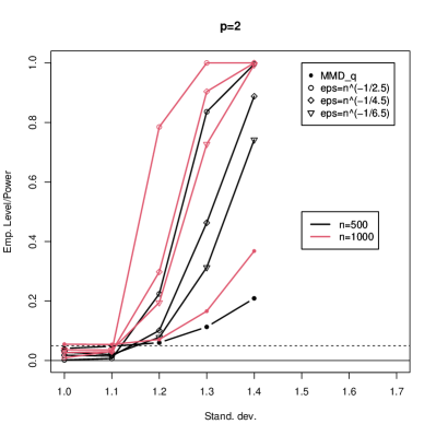
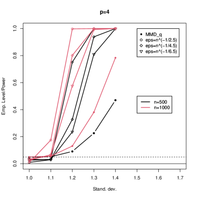
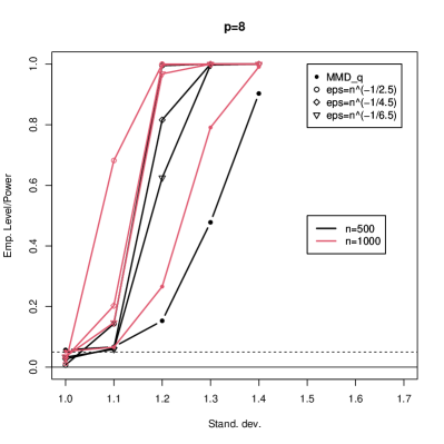
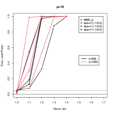
Figure 1: Empirical level and power of the tests based on $\mathcal{T}_{n}(\mathcal{M},P)$ and $\sqrt{n}\widehat{\operatorname{MMD}^{2}}_{q}(P_{\alpha_{n}},P)$ for dimension $p=2$ (top left), $p=4$ (top right), $p=8$ (bottom left), $p=16$ (bottom right) as well as for sample sizes $n=500$ (in black) and $n=1000$ (in red), different choices of $\epsilon_{n}$ and varying standard deviation. The rejection probabilities are estimated using $1000$ replications of the tests based on samples of size $n$. The dashed line indicates the significance level $0.05$.

For the two tests based on the statistics $\mathcal{T}_{n}(\mathcal{M},P)$ and $\sqrt{n}\widehat{\operatorname{MMD}^{2}}_{q}(P_{\alpha_{n}},P)$ with a level $5\%$, Figure 1 shows the empirical proportion of rejections of the null hypothesis $\mathcal{H}_{0}(\mathcal{M},P)$ for dimensions $p\in\{2,4,8,16\}$, sample sizes $n\in\{500,1000\}$ as well as for different choices of $\epsilon_{n}\in\{n^{-1/2.5},n^{-1/4.5},n^{-1/6.5}\}$. Note that the empirical proportion of rejections of $\mathcal{H}_{0}(\mathcal{M},P)$ for the case $\sigma=1.0$ is the empirical level of the tests. For $\sigma>1.0$, it is the empirical power of the tests.

First of all, we observe in Figure 1 that all tests keep their empirical level sufficiently well. Furthermore, if the convergence speed of $\epsilon_{n}$ to zero is decreasing, then the empirical power of the test based on $\mathcal{T}_{n}(\mathcal{M},P)$ is also decreasing. However, it is always higher than the empirical power of the test solely based on $\sqrt{n}\widehat{\operatorname{MMD}^{2}}_{q}(P_{\alpha_{n}},P)$. For any considered tuning parameter $\epsilon_{n}$, the test based on $\mathcal{T}_{n}(\mathcal{M},P)$ always outperforms the test based on $\sqrt{n}\widehat{\operatorname{MMD}^{2}}_{q}(P_{\alpha_{n}},P)$ for all considered sample sizes and dimensions. As expected, the empirical power of all tests is increasing with increasing sample size. It is also increasing for increasing dimension.

As a second example, define the family of competing models for the law of $X$ as

$$Y(\sigma)=\alpha_{0}{\bf 1}+diag(\sigma_{1},\ldots,\sigma_{p})Y\sim P_{\sigma},;\ Y\sim\mathcal{N}\left(0,I_{p}\right)$$

for some pre-specified marginal mean $\alpha_{0}\in\mathbb{R}$, where the marginal standard deviations are $\sigma_{1},\ldots,\sigma_{p}$, $\sigma:=(\sigma_{1},\ldots,\sigma_{p})$ and ${\bf 1}=(1,\ldots,1)$. If we fix $\alpha=0$ then the “optimal” parameters are $\sigma_{1}^{*}=\ldots=\sigma_{p}^{*}=1$ and $P=P_{\sigma^{*}}$, where $\sigma^{*}=(\sigma_{1}^{*},\ldots,\sigma_{p}^{*})$. Now, we vary the mean $\alpha_{0}$ of the competing model $Y(\sigma)$ by setting $\alpha_{0}\in\{0,\,0.1,\,0.2,\ldots,\,0.6\}$. As in the previous example, we consider the $p-$dimensional Gaussian kernel $k(X_{1},X_{2})=e^{-||X_{1}-X_{2}||^{2}/p}$ and set the significance level at $0.05$. Furthermore, we estimate $\sigma_{j}$ by the empirical standard deviation of the $j-$th marginal i.i.d. sample from $P$, namely $\sigma_{jn}^{2}=n^{-1}\sum_{i=1}^{n}(X_{ij}-\overline{X}_{ij})^{2}$. Thus, we use the two samples $(X_{1},\ldots,X_{n})$ and $\big{(}Y_{1}(\sigma_{n}),\ldots,Y_{n}(\sigma_{n})\big{)}$ from $P$ and $P_{\sigma_{n}}$ to test the null hypothesis $\mathcal{T}_{n}(\mathcal{M},P)$, where $\sigma_{n}:=(\sigma_{1n},\ldots,\sigma_{pn})$. In the simulation study, we set the number of Monte Carlo replications at $1000$, i.e., we compute the test statistics $\mathcal{T}_{n}(\mathcal{M},P)$ and $\sqrt{n}\widehat{\operatorname{MMD}^{2}}_{q}(P_{\sigma_{n}},P)$ each time using $1000$ random samples $(X_{1},\ldots,X_{n})$ and $(Y_{1}(\sigma_{n}),\ldots,Y_{n}(\sigma_{n}))$.

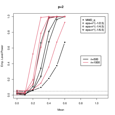
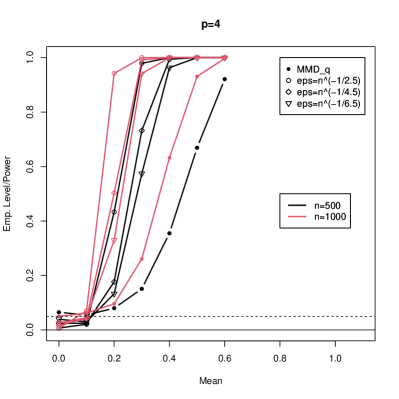
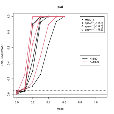
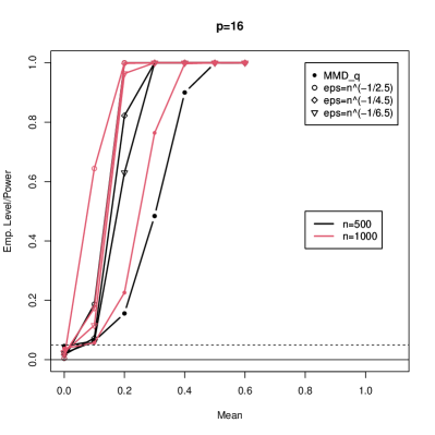
Figure 2: Empirical level and power of the tests based on $\mathcal{T}_{n}(\mathcal{M},P)$ and $\sqrt{n}\widehat{\operatorname{MMD}^{2}}_{q}(P_{\sigma_{n}},P)$ for dimension $p=2$ (top left), $p=4$ (top right), $p=8$ (bottom left), $p=16$ (bottom right) as well as for sample sizes $n=500$ (in black) and $n=1000$ (in red), different choices of $\epsilon_{n}$ and varying mean. The rejection probabilities are estimated using 1000 samples of size $n$. The dashed line indicates the significance level $0.05$.

For the two tests based on $\mathcal{T}_{n}(\mathcal{M},P)$ and $\sqrt{n}\widehat{\operatorname{MMD}^{2}}_{q}(P_{\sigma_{n}},P)$, Figure 2 shows the empirical proportion of rejections of the null hypothesis $\mathcal{H}_{0,\mathcal{M}}$ for dimensions $p\in\{2,4,8,16\}$, sample sizes $n\in\{500,1000\}$ as well as for different choices of $\epsilon_{n}\in\{n^{-1/2.5},n^{-1/4.5},n^{-1/6.5}\}$. Note that the empirical proportion of rejections of $\mathcal{H}_{0,\mathcal{M}}$ for the case $\alpha_{0}=0$ is the empirical level of the tests. For $\alpha_{0}>0$, it is the empirical power of the tests. Figure 2 shows that all considered tests keep their empirical level sufficiently well. Again, the tests based on $\mathcal{T}_{n}(\mathcal{M},P)$ are always more powerful than the test based on $\sqrt{n}\widehat{\operatorname{MMD}^{2}}_{q}(P_{\sigma_{n}},P)$ and similar conclusions as in the first example can be drawn.

In the third example, we consider two competing parametric models $\mathcal{M}_{1}$ and $\mathcal{M}_{2}$ for the law of $X$ and assume that the dimension $p$ is even. The first model $\mathcal{M}_{1}$ is defined by

$$Y_{i}(\alpha)=Y_{i}+\alpha\sim P_{\alpha},;\ Y_{i}\overset{i.i.d.}{\sim}\mathcal{N}\left(0,diag(1,\ldots,1,\sigma^{2},\ldots,\sigma^{2})\right)$$

for some pre-specified variance $\sigma^{2}$, where $\alpha=(\alpha_{1},\ldots,\alpha_{p})$. Thus, the first $p/2$ margins of $Y_{i}(\alpha)$ have variance $1$ and the remaining $p/2$ margins have variance $\sigma^{2}$. If $\sigma^{2}=1$, the model $\mathcal{M}_{1}$ coincides with the true model and the “optimal” parameter is ${\alpha_{\star}}=0$. The second model $\mathcal{M}_{2}$ is defined by

$$Z_{i}(\beta)=Z_{i}+\beta\sim P_{\beta}\,;\ Z_{i}\overset{i.i.d.}{\sim}\mathcal{N}\left(0,I_{p}\right)\,,$$

where $\beta=(\beta_{1},\ldots,\beta_{p})$. If $\beta=0$ then the model $\mathcal{M}_{2}$ also coincides with the the law of the DGP. Therefore, we may be in the degenerate situation, when the two competing models with optimal parameters coincide with the law of the DGP. Similar to the first example, we vary the standard deviation $\sigma$ by setting $\sigma\in\{1.0,\,1.1,\,1.2,\,1.3,\,1.4\}$. Further, we estimate $\alpha$ and $\beta$ by the empirical mean of the i.i.d. sample from $P$, $\alpha_{n}=\beta_{n}=n^{-1}\sum_{i=1}^{n}X_{i}$. Then, we independently generate the two samples $\big{(}Y_{1}(\alpha_{n}),\ldots,Y_{n}(\alpha_{n})\big{)}$ and $\big{(}Z_{1}(\beta_{n}),\ldots,Z_{n}(\beta_{n})\big{)}$ to test the null hypothesis $\mathcal{H}_{0,\mathcal{M}_{1},\mathcal{M}_{2}}:\operatorname{MMD}(P_{\alpha_{\star}},P)=\operatorname{MMD}(Q_{\beta_{\star}},P)$. In the simulation study, we set the number of Monte Carlo replications to $1000$ and compute each time the test statistics $\mathcal{T}_{n}(\mathcal{M}_{1},\mathcal{M}_{2},P)$ each time using $1000$ random samples $(X_{1},\ldots,X_{n})$, $\big{(}Y_{1}(\alpha_{n}),\ldots,Y_{n}(\alpha_{n})\big{)}$ and $\big{(}Z_{1}(\beta_{n}),\ldots,Z_{n}(\beta_{n})\big{)}$. As a comparison, we also provide provide the level/power of a test of $\mathcal{H}_{0,\mathcal{M}_{1},\mathcal{M}_{2}}$ which is solely based on $\sqrt{n}\big{(}\widehat{\operatorname{MMD}^{2}}_{q}(P_{\alpha_{n}},P)-\widehat{\operatorname{MMD}^{2}}_{q}(P_{\beta_{n}},P)\big{)}$.

For the two tests based on the statistics $\mathcal{T}_{n}(\mathcal{M}_{1},\mathcal{M}_{2},P)$ and $\sqrt{n}\big{(}\widehat{\operatorname{MMD}^{2}}_{q}(P_{\alpha_{n}},P)-\widehat{\operatorname{MMD}^{2}}_{q}(P_{\beta_{n}},P)\big{)}$, Figure 3 shows the empirical proportion of rejections of the null hypothesis $\mathcal{H}_{0,\mathcal{M}_{1},\mathcal{M}_{2}}$ for dimensions $p\in\{2,4,8,16\}$, sample sizes $n\in\{500,1000\}$ as well as for different choices of $\epsilon_{n}\in\{n^{-1/2.5},n^{-1/4.5},n^{-1/6.5}\}$. Note that the empirical proportion of rejection of $\mathcal{H}_{0,\mathcal{M}_{1},\mathcal{M}_{2}}$ for the case $\sigma=1.0$ is the empirical level of the tests. For $\sigma>1.0$, it is the empirical power of the tests.

First of all, we observe in Figure 3 that all tests keep their empirical level sufficiently well. Furthermore, if the convergence speed of $\epsilon_{n}$ to zero is decreasing, then the empirical power of the test based on $\mathcal{T}_{n}(\mathcal{M},P)$ is also decreasing. However, it is always higher than the empirical power of the test solely based on $\sqrt{n}\widehat{\operatorname{MMD}^{2}}_{q}(P_{\alpha_{n}},P)$. For any considered tuning parameter $\epsilon_{n}$, the test based on $\mathcal{T}_{n}(\mathcal{M},P)$ always outperforms the test based on the competitor test statistic $\sqrt{n}\widehat{\operatorname{MMD}^{2}}_{q}(P_{\alpha_{n}},P)$ for all considered sample sizes and dimensions. As expected, the empirical power of all tests is increasing with increasing sample size. As we have already observed, it is also increasing for increasing dimension.

For the fourth example, we modify the third example to avoid the degenerate case. Now, the models $\mathcal{M}_{1}$ and $\mathcal{M}_{2}$ are given by

$$Y_{i}(\alpha)=Y_{i}+\alpha\sim P_{\alpha},;\ Y_{i}\overset{i.i.d.}{\sim}\mathcal{N}\left(0,diag(1.2^{2},\ldots,1.2^{2},\sigma^{2},\ldots,\sigma^{2})\right),\;\text{and}$$

$$Z_{i}(\beta)=Z_{i}+\beta\sim P_{\beta}\,;\ Z_{i}\overset{i.i.d.}{\sim}\mathcal{N}\left(0,1.2^{2}I_{p}\right)\,,$$

respectively. Thus, both models cannot coincide with the DGP, reflecting the non-degenerate case. However, for $\sigma=1.2$, they coincide and are therefore equally far away from the DGP. We vary the standard deviation $\sigma$ by setting $\sigma\in\{1.2,\,1.3,\,1.4,\,1.5,\,1.6\}$.

For the two tests based on the statistics $\mathcal{T}_{n}(\mathcal{M}_{1},\mathcal{M}_{2},P)$ and $\sqrt{n}\big{(}\widehat{\operatorname{MMD}^{2}}_{q}(P_{\alpha_{n}},P)-\widehat{\operatorname{MMD}^{2}}_{q}(P_{\beta_{n}},P)\big{)}$, Figure 4 shows the empirical proportion of rejections of the null hypothesis $\mathcal{H}_{0,\mathcal{M}_{1},\mathcal{M}_{2}}$ for dimensions $p\in\{2,4,8,16\}$, sample sizes $n\in\{500,1000\}$ as well as for different choices of $\epsilon_{n}\in\{n^{-1/2.5},n^{-1/4.5},n^{-1/6.5}\}$. Note that the empirical proportion of rejections of $\mathcal{H}_{0,\mathcal{M}_{1},\mathcal{M}_{2}}$ for the case $\sigma=1.2$ is the empirical level of the tests. For $\sigma>1.2$, it is the empirical power of the tests. In Figure 4, we clearly observe that the test based on $\mathcal{T}_{n}(\mathcal{M}_{1},\mathcal{M}_{2},P)$ is again more powerful than a test based $\sqrt{n}\big{(}\widehat{\operatorname{MMD}^{2}}_{q}(P_{\alpha_{n}},P)-\widehat{\operatorname{MMD}^{2}}_{q}(P_{\beta_{n}},P)\big{)}$, even in the non-degenerate case. Further, both tests are more powerful in comparison to our tests studied in the degenerate case (Example 3).

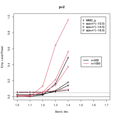
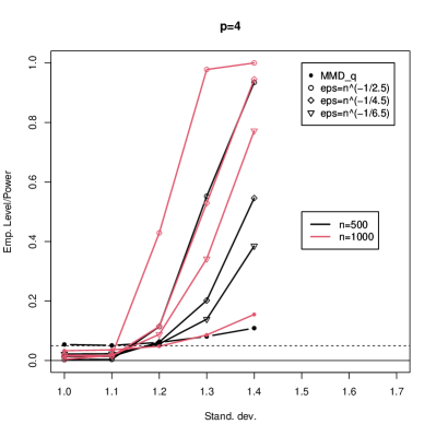
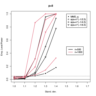
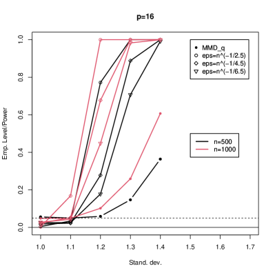
Figure 3: Degenerate case for comparison of two models: Empirical level and power of the tests based on $\mathcal{T}_{n}(\mathcal{M}_{1},\mathcal{M}_{2},P)$ and $\sqrt{n}\big{(}\widehat{\operatorname{MMD}^{2}}_{q}(P_{\alpha_{n}},P)-\widehat{\operatorname{MMD}^{2}}_{q}(P_{\beta_{n}},P)\big{)}$ for dimension $p=2$ (top left), $p=4$ (top right), $p=8$ (bottom left), $p=16$ (bottom right) as well as for sample sizes $n=500$ (in black) and $n=1000$ (in red), different choices of $\epsilon_{n}$ and varying standard deviation $\sigma$ in Model $\mathcal{M}_{1}$. Model $\mathcal{M}_{2}$ always coincides with the true model ($\beta=0$). The rejection probabilities are estimated using $1000$ replications of the tests based on samples of size $n$. The dashed line indicates the significance level $0.05$.

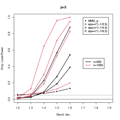
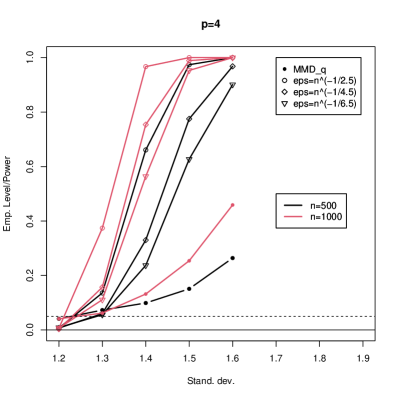
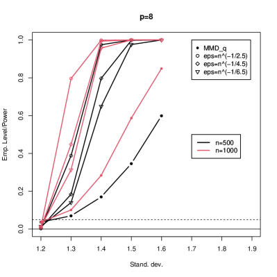
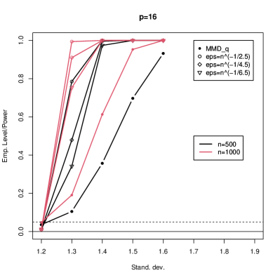
Figure 4: Non-degenerate case for comparison of two models: Empirical level and power of the tests based on $\mathcal{T}_{n}(\mathcal{M}_{1},\mathcal{M}_{2},P)$ and $\sqrt{n}\big{(}\widehat{\operatorname{MMD}^{2}}_{q}(P_{\alpha_{n}},P)-\widehat{\operatorname{MMD}^{2}}_{q}(P_{\beta_{n}},P)\big{)}$ for dimension $p=2$ (top left), $p=4$ (top right), $p=8$ (bottom left), $p=16$ (bottom right) as well as for sample sizes $n=500$ (in black) and $n=1000$ (in red), different choices of $\epsilon_{n}$ and varying standard deviation in Model $\mathcal{M}_{1}$. Both models do not coincide with the true model. The rejection probabilities are estimated using $1000$ replications of the tests based on samples of size $n$. The dashed line indicates the significance level $0.05$.

6 Conclusion and Outlook

We provided a novel MMD-based model specification and model selection test when model parameters are estimated in a first-stage. The tests circumvent the major difficulty of computing the critical values of a complicated asymptotic distribution, but instead simply require to resort to the critical values of the standard normal distribution. Moreover, since our testing procedures are also valid when no parameter estimation is conducted, we thereby mitigate one of the major inconveniences when working with the two sample test proposed by [24].

Both proposed test statistics depend on a tuning parameter, whose “optimal” choice is still an open problem that may be investigated in the future. Moreover, it remains future work to derive certain properties of our testing procedures, such as the local power and uniformity of convergence over sets of DGPs.

Moreover, for our model selection test, we have to assume that the “pseudo-true” values of the suggested models for the DGP are also the minimizers of the MMD distance. Due to the wide applicability of our testing procedure, it might be desirable to avoid this requirement. For example, in practice, it might be the case that competing models are fitted to the observed data via different statistical methods, which then often poses the question of finding a suitable statistical procedure that allows to compare these models. Here, our test for model comparison might act as a common ground of truth, since it can be applied to very general mathematical frameworks. However, it might be questionable that the obtained “pseudo-true” values are actually also the minimizers w.r.t. the MMD distance, preventing a justified application of our model selection test. A remedy to this shortcoming might lie in bootstrapping the critical values of our test statistic, because it usually requires less strict assumptions. Unfortunately, it is well known that bootstrapping degenerate $U$-statistic is a difficult task and workarounds as the permutation bootstrap proposed in [1] seem to not be suited for such applications. Thus, it remains an interesting open question to find a feasible bootstrap procedure for our model selection test that does not require that the “pseudo-true” values are the minimizers w.r.t. the MMD distance.

Finally, [16] recently investigated parameter estimation based on the MMD distance, provided dependent input data. Since our test statistics are basically composed of $U$-statistics, future research might be concerned with relaxing the assumption of i.i.d. observations in the application of our MMD-based model specification and model selection test by resorting to the vast literature on $U$-statistics of dependent data.

Appendix A Proofs

A.1 Proof of Lemma 1

1. A first order Taylor expansion yields

   $$\widehat{\operatorname{MMD}^{2}}(P_{\alpha_{n}},P)=\frac{1}{n(n-1)}\sum_{\begin{subarray}{c}i,j=1\\ i\not=j\end{subarray}}^{n}\big{\{}h(X_{i},U_{i},X_{j},U_{j};{\alpha_{\star}})+\nabla_{\alpha^{\intercal}}h(X_{i},U_{i},X_{j},U_{j};{\alpha_{\star}}).({\alpha_{n}}-{\alpha_{\star}})\big{\}}$$ (16)

   $$+ O_{\mathbb{P}}(\|{\alpha_{n}}-{\alpha_{\star}}\|^{2}).\hskip 284.52756pt$$

   Note that the remainder term is due to Assumption 5. The weak convergence of $\sqrt{n}\big{\{}\widehat{\operatorname{MMD}^{2}}(P_{\alpha_{n}},P)-\operatorname{MMD}^{2}(P_{\alpha_{\star}},P)\big{\}}$ is a direct consequence of Assumption 3 in addition to Fubini’s theorem applied to $\nabla_{\alpha}h$ at $\alpha={\alpha_{\star}}$ (second part of Assumption 5). The convergence of the estimated variance $\hat{\sigma}^{2}_{\alpha_{n}}$ is easily obtained by a first order Taylor expansion of the maps $\alpha\mapsto g_{\alpha}(X_{i},U_{i},X_{j},U_{j},X_{k},U_{k})$ defined in (10) around ${\alpha_{\star}}$, for every triplet of indices $(i,j,k)$, $i\neq j\neq k$. The remainder term is negligible under Assumption 5.

2. With obvious notations, rewrite (16) as

   $$\widehat{\operatorname{MMD}^{2}}(P_{\alpha_{n}},P)=\mathcal{U}^{(1)}_{n}h(\cdot;{\alpha_{\star}})+\mathcal{U}^{(1)}_{n}\nabla_{\alpha^{\intercal}}h(\cdot;{\alpha_{\star}}).({\alpha_{n}}-{\alpha_{\star}})+O_{\mathbb{P}}(n^{-1}).$$

   Since $\mathcal{U}^{(1)}_{n}h(\cdot;{\alpha_{\star}})$ is a degenerate $U$-statistic, it is $O_{\mathbb{P}}(n^{-1})$. Moreover, the mean of the $U$-statistic $\mathcal{U}^{(1)}_{n}\nabla_{\alpha^{\intercal}}h(\cdot;{\alpha_{\star}})$ is zero because

   $$\mathbb{E}\big{[}\nabla_{\alpha}h(X_{i},U_{i},X_{j},U_{j};{\alpha_{\star}})\big{]}=\nabla_{\alpha}\mathbb{E}\big{[}h(X_{i},U_{i},X_{j},U_{j};{\alpha_{\star}})\big{]}=\nabla_{\alpha}\operatorname{MMD}^{2}(P_{\alpha},P)|_{\alpha={\alpha_{\star}}}=0.$$

   Thus, the $U$-statistic $\mathcal{U}^{(1)}_{n}\nabla_{\alpha^{\intercal}}h(\cdot;{\alpha_{\star}})$ is $O_{\mathbb{P}}(n^{-1/2})$. This implies $\sqrt{n}\,\widehat{\operatorname{MMD}^{2}}(P_{\alpha_{n}},P)=O_{\mathbb{P}}(n^{-1/2})$, the announced result.

   Concerning the asymptotic variance, a Taylor expansion of $\alpha\mapsto g_{\alpha}$ around ${\alpha_{\star}}$ and Assumption 5 yield

   $$\hat{\sigma}^{2}_{\alpha_{n}}=\mathcal{U}^{(1)}_{n}g_{\alpha_{n}}=\mathcal{U}^{(1)}_{n}g_{\alpha_{\star}}+\mathcal{U}^{(1)}_{n}\nabla_{\alpha^{\intercal}}g_{\alpha_{\star}}.({\alpha_{n}}-{\alpha_{\star}})+O_{P}\big{(}\|{\alpha_{n}}-{\alpha_{\star}}\|^{2}\big{)}.$$

   Since $\mathcal{U}^{(1)}_{n}g_{\alpha_{\star}}$ is a degenerate $U$-statistic, this term is $O_{\mathbb{P}}(n^{-1})$.

   Moreover, $\mathcal{U}^{(1)}_{n}\nabla_{\alpha}g_{\alpha_{\star}}$ tends in probability to $\nabla_{\alpha}\mathbb{E}\big{[}g_{\alpha_{\star}}(X_{1},U_{1},X_{2},U_{2},X_{3},U_{3})\big{]}$ (Assumption 5), that is zero because $\alpha\mapsto\mathbb{E}\big{[}g_{\alpha}(X_{1},U_{1},X_{2},U_{2},X_{3},U_{3})\big{]}$ is minimal when $\alpha={\alpha_{\star}}$. This implies that the $U$-statistic $\mathcal{U}^{(1)}_{n}\nabla_{\alpha}g_{\alpha_{\star}}$ is $O_{\mathbb{P}}(n^{-1/2})$. Globally, we get $\hat{\sigma}^{2}_{\alpha_{n}}=O_{\mathbb{P}}(n^{-1})$.

3. The positivity of $\sigma_{q,{\alpha_{\star}}}$ had already been noted at the end of Section 3.2. The rest can be proved exactly as for (i).

A.2 Proof of Theorem 3.1

1. Note that

   $$\sqrt{n}\frac{\widehat{\operatorname{MMD}^{2}}_{\epsilon_{n}}(P_{\alpha_{n}},P)}{\hat{\sigma}_{{\alpha_{n}}}+\epsilon_{n}\hat{\sigma}_{q,{\alpha_{n}}}}=\frac{\sqrt{n}\,\widehat{\operatorname{MMD}^{2}}(P_{\alpha_{n}},P)}{\hat{\sigma}_{{\alpha_{n}}}+\epsilon_{n}\hat{\sigma}_{q,{\alpha_{n}}}}+\frac{n^{1/2}\epsilon_{n}\;\sqrt{n}\,\widehat{\operatorname{MMD}^{2}}_{q}(P_{\alpha_{n}},P)}{n^{1/2}\hat{\sigma}_{{\alpha_{n}}}+n^{1/2}\epsilon_{n}\hat{\sigma}_{q,{\alpha_{n}}}}\cdot$$

   Invoking Lemma 1, we obtain

   $$\frac{\sqrt{n}\,\widehat{\operatorname{MMD}^{2}}(P_{\alpha_{n}},P)}{\hat{\sigma}_{{\alpha_{n}}}+\epsilon_{n}\hat{\sigma}_{q,{\alpha_{n}}}}=\frac{O_{\mathbb{P}}(n^{-1/2})}{O_{p}(n^{-1/2})+\epsilon_{n}\hat{\sigma}_{q,{\alpha_{n}}}}=\frac{O_{\mathbb{P}}(1)}{O_{p}(1)+n^{1/2}\epsilon_{n}\hat{\sigma}_{q,{\alpha_{n}}}}.$$

   Since $\epsilon_{n}n^{1/2}\to\infty$ by assumption and $\hat{\sigma}_{q,{\alpha_{n}}}\rightarrow\sigma_{q,{\alpha_{\star}}}>0$, this yields

   $$\frac{\sqrt{n}\,\widehat{\operatorname{MMD}^{2}}(P_{\alpha_{n}},P)}{\hat{\sigma}_{n,{\alpha_{n}}}+\epsilon_{n}\hat{\sigma}_{q,{\alpha_{n}}}}=o_{\mathbb{P}}(1).$$

   Again, by Lemma 1 and the consistency of $\hat{\sigma}_{q,{\alpha_{n}}}$, we have $n^{1/2}\epsilon_{n}\hat{\sigma}_{q,{\alpha_{n}}}\rightarrow\infty$, when $n^{1/2}\hat{\sigma}_{{\alpha_{n}}}=O_{\mathbb{P}}(1)$. This provides

   $$\frac{n^{1/2}\epsilon_{n}\sqrt{n}\,\widehat{\operatorname{MMD}^{2}}_{q}(P_{\alpha_{n}},P)}{n^{1/2}\hat{\sigma}_{{\alpha_{n}}}+n^{1/2}\epsilon_{n}\hat{\sigma}_{q,{\alpha_{n}}}}=\frac{\sqrt{n}\,\widehat{\operatorname{MMD}^{2}}_{q}(P_{\alpha_{n}},P)}{\hat{\sigma}_{q,{\alpha_{n}}}}+o_{\mathbb{P}}(1)\stackrel{{\scriptstyle\text{law}}}{{\longrightarrow}}\frac{\mathcal{N}(0,\sigma^{2}_{q,{\alpha_{\star}}})}{\sigma_{q,{\alpha_{\star}}}}\sim\mathcal{N}(0,1),$$

   which proves the claim.

2. When $P_{\alpha_{\star}}\not=P$, $\sqrt{n}\big{\{}\widehat{\operatorname{MMD}^{2}}(P_{\alpha_{n}},P)-\operatorname{MMD}^{2}(P_{\alpha_{\star}},P)\big{\}}$ weakly converges to a non-degenerate random variable and $\hat{\sigma}_{\alpha_{n}}\to\sigma_{\alpha_{\star}}>0$, due to Lemma 1. Therefore, the denominator of $\mathcal{T}_{n}$ tends to $\sigma_{\alpha_{\star}}$ in probability and

   $$\frac{\sqrt{n}\,\widehat{\operatorname{MMD}^{2}}(P_{\alpha_{n}},P)}{\hat{\sigma}_{{\alpha_{n}}}+\epsilon_{n}\hat{\sigma}_{q,{\alpha_{n}}}}=\sqrt{n}\frac{\operatorname{MMD}^{2}(P_{\alpha_{\star}},P)}{\sigma_{\alpha_{\star}}}+O_{\mathbb{P}}(1).$$

   Similarly, we have

   $$\epsilon_{n}\frac{\sqrt{n}\,\widehat{\operatorname{MMD}^{2}}_{q}(P_{\alpha_{n}},P)}{\hat{\sigma}_{{\alpha_{n}}}+\epsilon_{n}\hat{\sigma}_{q,{\alpha_{n}}}}=\epsilon_{n}\sqrt{n}\frac{\operatorname{MMD}^{2}(P_{\alpha_{\star}},P)}{\sigma_{\alpha_{\star}}}+o_{\mathbb{P}}(1).$$

   This yields

   $$\sqrt{n}\frac{\widehat{\operatorname{MMD}^{2}}_{\epsilon_{n}}(P_{\alpha_{n}},P)}{\hat{\sigma}_{{\alpha_{n}}}+\epsilon_{n}\hat{\sigma}_{q,{\alpha_{n}}}}=O_{p}(1)+\sqrt{n}(1+\epsilon_{n})\frac{\operatorname{MMD}^{2}(P_{\alpha_{\star}},P)}{\sigma_{\alpha_{\star}}},$$

   which implies the claim since $\operatorname{MMD}^{2}(P_{\alpha_{\star}},P)>0$.

A.3 Proof of Lemma 2

1. Note that

   $$\sqrt{n}\big{\{}\widehat{\operatorname{MMD}^{2}}(P_{\alpha_{n}},P)-\operatorname{MMD}^{2}(P_{\alpha_{\star}},P)\big{\}}$$

   $$= \sqrt{n}\big{\{}\widehat{\operatorname{MMD}^{2}}(P_{\alpha_{n}},P)-\operatorname{MMD}^{2}(P_{\alpha_{n}},P)-\widehat{\operatorname{MMD}^{2}}(P_{\alpha_{\star}},P)+\operatorname{MMD}^{2}(P_{\alpha_{\star}},P)$$

   $$+ \widehat{\operatorname{MMD}^{2}}(P_{\alpha_{\star}},P)-\operatorname{MMD}^{2}(P_{\alpha_{\star}},P)+\operatorname{MMD}^{2}(P_{\alpha_{n}},P)-\operatorname{MMD}^{2}(P_{\alpha_{\star}},P)\big{\}}$$

   $$= \sqrt{n}(\mathcal{U}^{(1)}_{n}-\mathbb{P})(h(\cdot;{\alpha_{n}})-h(\cdot;{\alpha_{\star}}))+\sqrt{n}(\mathcal{U}^{(1)}_{n}-\mathbb{P})h(\cdot;{\alpha_{\star}})$$

   $$+ \sqrt{n}\nabla_{\alpha^{\intercal}}\operatorname{MMD}^{2}(P_{\alpha},P)|_{\alpha={\alpha_{\star}}}({\alpha_{n}}-{\alpha_{\star}})+\sqrt{n}\,o_{\mathbb{P}}(\|{\alpha_{n}}-{\alpha_{\star}}\|),$$

   by a Taylor expansion of $\alpha\mapsto\operatorname{MMD}^{2}(P_{\alpha},P)$. Since the process $\sqrt{n}(\mathcal{U}^{(1)}_{n}-\mathbb{P})$, indexed by $\mathcal{F}$, is asymptotically equicontinuous by Assumption 6 and $\|h(\cdot;{\alpha_{n}})-h(\cdot;{\alpha_{\star}})\|_{L_{2}(P\otimes P_{U}\otimes P\otimes P_{U})}\to 0$ in probability, we have $\sqrt{n}(\mathcal{U}^{(1)}_{n}-\mathbb{P})\big{(}h(\cdot;{\alpha_{n}})-h(\cdot;{\alpha_{\star}})\big{)}$ is $o_{p}(1)$. Moreover, by [5, Theorem 4.9], $\sqrt{n}(\mathcal{U}^{(1)}_{n}-\mathbb{P})h(\cdot;{\alpha_{\star}})$ converges in law towards a normal random variable whose variance is

   $$\sigma_{\alpha_{\star}}^{2}=\operatorname{Var}\Big{(}2\mathbb{E}_{X_{2},U_{2}}\big{[}h(X_{1},U_{1},X_{2},U_{2};{\alpha_{\star}})|\,X_{1},U_{1}\big{]}\Big{)}.$$

   By assumption, $\sqrt{n}\nabla_{\alpha^{\intercal}}\operatorname{MMD}^{2}(P_{\alpha},P)|_{\alpha={\alpha_{\star}}}({\alpha_{n}}-{\alpha_{\star}})$ converges to $\nabla_{\alpha^{\intercal}}\operatorname{MMD}^{2}(P_{\alpha},P)|_{\alpha={\alpha_{\star}}}V_{\alpha_{\star}}$ and the joint convergence follows from Assumption 3. The fourth term is clearly $o_{\mathbb{P}}(1)$, since $\|{\alpha_{n}}-{\alpha_{\star}}\|=O_{\mathbb{P}}(n^{-1/2})$. Thus

   $$\sqrt{n}\big{\{}\widehat{\operatorname{MMD}^{2}}(P_{\alpha_{n}},P)-\operatorname{MMD}^{2}(P_{\alpha_{\star}},P)\big{\}}\stackrel{{\scriptstyle\text{law}}}{{\longrightarrow}}Z_{\alpha_{\star}}+\nabla_{\alpha^{\intercal}}\operatorname{MMD}^{2}(P_{\alpha},P)|_{\alpha={\alpha_{\star}}}V_{\alpha_{\star}},$$

   Furthermore, $\hat{\sigma}^{2}_{{\alpha_{n}}}=\mathcal{U}^{(1)}_{n}g_{\alpha_{n}}-4\Big{\{}\widehat{\operatorname{MMD}^{2}}(P_{\alpha_{n}},P)\Big{\}}^{2}$. We have just deduced that $\widehat{\operatorname{MMD}^{2}}(P_{\alpha_{n}},P)$ converges to $\operatorname{MMD}^{2}(P_{\alpha_{\star}},P)$ in probability. Similarly, since $\sqrt{n}(\mathcal{U}^{(1)}_{n}-\mathbb{P})$ indexed by $\mathcal{G}$ converges to a Gaussian limit and $\|g_{\alpha_{n}}-g_{\alpha_{\star}}\|_{L_{2}(\otimes_{i=1}^{3}P\otimes P_{U})}\to 0$ in probability, we have

   $$\mathcal{U}^{(1)}_{n}g_{\alpha_{n}}=\mathbb{E}_{(X^{\prime},U^{\prime},X^{\prime\prime},U^{\prime\prime},X^{\prime\prime\prime},U^{\prime\prime\prime})\sim\otimes_{i=1}^{3}P\otimes P_{U}}[g_{\alpha_{n}}(X^{\prime},U^{\prime},X^{\prime\prime},U^{\prime\prime},X^{\prime\prime\prime},U^{\prime\prime\prime})]+o_{\mathbb{P}}(1).$$

   and

   $$\Big{|}\mathbb{E}_{(X^{\prime},U^{\prime},X^{\prime\prime},U^{\prime\prime},X^{\prime\prime\prime},U^{\prime\prime\prime})\sim\otimes_{i=1}^{3}P\otimes P_{U}}\left[g_{\alpha_{n}}(X^{\prime},U^{\prime},X^{\prime\prime},U^{\prime\prime},X^{\prime\prime\prime},U^{\prime\prime\prime})-g_{\alpha_{\star}}(X^{\prime},U^{\prime},X^{\prime\prime},U^{\prime\prime},X^{\prime\prime\prime},U^{\prime\prime\prime})\right]\Big{|}$$

   $$\leq\|g_{\alpha_{n}}-g_{\alpha_{\star}}\|_{L_{2}(\otimes_{i=1}^{3}P\otimes P_{U})}\stackrel{{\scriptstyle P}}{{\rightarrow}}0.$$

   Thus, this yields

   $$\mathcal{U}^{(1)}_{n}g_{\alpha_{n}}=\mathbb{E}[g_{\alpha_{\star}}(X_{1},U_{1},X_{2},U_{2},X_{3},U_{3})]+o_{\mathbb{P}}(1),$$

   proving that $\hat{\sigma}_{\alpha_{n}}^{2}\to\sigma^{2}_{\alpha_{\star}}$ in probability.

2. Obviously, when $P_{\alpha_{\star}}=P$, $\nabla_{\alpha}\operatorname{MMD}^{2}(P_{\alpha},P)|_{\alpha={\alpha_{\star}}}=0$ since ${\alpha_{\star}}$ belongs to the interior of $\Theta_{\alpha}$ and is the argmin of $\alpha\mapsto\operatorname{MMD}^{2}(P_{\alpha},P)$. Moreover, $\mathcal{U}^{(1)}_{n}h(\cdot;{\alpha_{\star}})=O_{\mathbb{P}}(n^{-1})$ by standard $U$-statistic arguments, because $h(\cdot;{\alpha_{\star}})$ is now a degenerate $U$-statistic kernel. Note that, by Assumption 2, $\sqrt{n}\,\operatorname{MMD}^{2}(P_{\alpha_{n}},P)=O_{\mathbb{P}}(n^{-1/2})$. Indeed, a second-order limited expansion of $\alpha\mapsto\operatorname{MMD}^{2}(P_{\alpha},P)$ around ${\alpha_{\star}}$ yields

   $$\operatorname{MMD}^{2}(P_{\alpha_{n}},P)=({\alpha_{n}}-{\alpha_{\star}})^{\intercal}\nabla^{2}_{\alpha,\alpha^{\intercal}}\operatorname{MMD}^{2}(P_{\alpha},P)|_{\alpha={\alpha_{\star}}}({\alpha_{n}}-{\alpha_{\star}})+o_{p}\left(\|{\alpha_{n}}-{\alpha_{\star}}\|^{2}\right)=O_{p}\left(\|{\alpha_{n}}-{\alpha_{\star}}\|^{2}\right),$$

   which is $O_{\mathbb{P}}(n^{-1})$. Let us decompose the quantity of interest as

   $$\sqrt{n}\,\widehat{\operatorname{MMD}^{2}}(P_{\alpha_{n}},P)=\sqrt{n}\,\mathcal{U}^{(1)}_{n}h(\cdot;{\alpha_{n}})=\sqrt{n}\,\mathcal{U}^{(1)}_{n}\big{(}h(\cdot;{\alpha_{n}})-h(\cdot;{\alpha_{\star}})\big{)}+O_{\mathbb{P}}(n^{-1/2}).$$

   Thus, it remains to prove that $\sqrt{n}\,\mathcal{U}^{(1)}_{n}\big{(}h(\cdot;{\alpha_{n}})-h(\cdot;{\alpha_{\star}})\big{)}=O_{\mathbb{P}}(n^{-1/2})$. To this aim, we will use the asymptotic equicontinuity of degenerate $U$-statistic kernels. Obviously, for any $\alpha={\alpha_{\star}}$, $h(\cdot;\alpha)-h(\cdot;{\alpha_{\star}})$ is generally not a degenerate $U$-statistic kernel. Nonetheless, we can rewrite

   $$\sqrt{n}\,\mathcal{U}^{(1)}_{n}\big{(}h(\cdot;{\alpha_{n}})-h(\cdot;{\alpha_{\star}})\big{)}=\frac{\sqrt{n}}{n(n-1)}\sum_{\begin{subarray}{c}i,j=1\\ i\not=j\end{subarray}}^{n}\Big{\{}h\big{(}(X_{i},F(U_{i};{\alpha_{n}})),(X_{j},F(U_{j};{\alpha_{n}}))\big{)}-\tilde{h}_{\alpha_{n}}(X_{i},F(U_{i};{\alpha_{n}}))$$ (17)

   $$- \tilde{h}_{\alpha_{n}}\big{(}X_{j},F(U_{j};{\alpha_{n}})\big{)}+\operatorname{MMD}^{2}(P_{\alpha_{n}},P)-h\big{(}(X_{i},F(U_{i};{\alpha_{\star}})),(X_{j},F(U_{j};{\alpha_{\star}}))\big{)}\Big{\}}$$

   $$+ \frac{\sqrt{n}}{n(n-1)}\sum_{\begin{subarray}{c}i,j=1\\ i\not=j\end{subarray}}^{n}\Big{\{}\tilde{h}_{\alpha_{n}}\big{(}X_{i},F(U_{i};{\alpha_{n}})\big{)}+\tilde{h}_{\alpha_{n}}\big{(}X_{j},F(U_{j};{\alpha_{n}})\big{)}\Big{\}}-\sqrt{n}\,\operatorname{MMD}^{2}(P_{\alpha_{n}},P)$$

   $$= \frac{\sqrt{n}}{n(n-1)}\sum_{\begin{subarray}{c}i,j=1\\ i\not=j\end{subarray}}^{n}\big{\{}\psi(X_{i},U_{i},X_{j},U_{j};{\alpha_{n}})-\psi(X_{i},U_{i},X_{j},U_{j};{\alpha_{\star}})\big{\}}$$

   $$+ \frac{2\sqrt{n}}{n}\sum_{i=1}^{n}\tilde{h}_{\alpha_{n}}\big{(}X_{i},F(U_{i};{\alpha_{n}})\big{)}+O_{\mathbb{P}}(n^{-1/2}),\hskip 199.16928pt$$

   by setting

   $$\psi(x_{1},u_{1},x_{2},u_{2};\alpha):=h(x_{1},u_{1},x_{2},u_{2};\alpha)-\tilde{h}_{\alpha}\big{(}x_{1},F(u_{1};\alpha)\big{)}-\tilde{h}_{\alpha}(x_{2},F(u_{2};\alpha)\big{)}+\operatorname{MMD}^{2}(P_{\alpha},P).$$

   Note that $\psi(x_{1},u_{1},x_{2},u_{2};{\alpha_{\star}})=h(x_{1},u_{1},x_{2},u_{2};{\alpha_{\star}})$ because $\tilde{h}_{\alpha_{\star}}\big{(}x,y)=0$ for every $(x,y)$, when $P=P_{\alpha_{\star}}$. Moreover, the $U$-statistic $\mathcal{U}^{(1)}_{n}\psi(\cdot;\alpha)$ is now degenerate, for every $\alpha\in\Theta_{\alpha}$. For any $\epsilon>0$ and any positive constants $\delta_{k}$, $k\in\{1,2\}$, we get

   $$\mathbb{P}\bigg{(}\Big{|}\frac{\sqrt{n}}{n(n-1)}\sum_{\begin{subarray}{c}i,j=1\\ i\not=j\end{subarray}}^{n}\big{\{}\psi(X_{i},U_{i},X_{j},U_{j};{\alpha_{n}})-\psi(X_{i},U_{i},X_{j},U_{j};{\alpha_{\star}})\big{\}}\Big{|}>n^{-1/2}\epsilon\bigg{)}$$

   $$\leq \mathbb{P}\Big{(}\sup_{f,g\in\mathcal{F}_{c}\|f-g\|_{L_{2}(\otimes_{i=1}^{2}P\otimes P_{u})}<\delta_{2}}\big{|}n(\mathcal{U}^{(1)}_{n}-\mathbb{P})(f-g)\big{|}>\epsilon\Big{)}+\mathbb{P}(\|{\alpha_{n}}-{\alpha_{\star}}\|\geq\delta_{1})$$

   $$+ \mathbb{P}\Big{(}\|\psi(\cdot;{\alpha_{n}})-\psi(\cdot;{\alpha_{\star}})\|_{L_{2}(\otimes_{i=1}^{2}(P\otimes P_{U}))}\geq\delta_{2},\|{\alpha_{n}}-{\alpha_{\star}}\|<\delta_{1}\Big{)}=:T_{1}+T_{2}+T_{3}.$$

   By the asymptotic equicontinuity of $n(\mathcal{U}^{(1)}_{n}-\mathbb{P})$ indexed by $\mathcal{F}_{c}$ (Assumption 8), there exists $\delta_{2}$ s.t. $T_{1}$ is arbitrarily small for $n$ sufficiently large. Since $\|\psi(\cdot;{\alpha_{n}})-\psi(\cdot;{\alpha_{\star}})\|_{L_{2}(\otimes_{i=1}^{2}(P\otimes P_{U}))}\leq 4\|h(\cdot;{\alpha_{n}})-h(\cdot;{\alpha_{\star}})\|_{L_{2}(\otimes_{i=1}^{2}(P\otimes P_{U}))}$ that tends to zero in probability, $\delta_{1}$ can be chosen so that $T_{2}$ and $T_{3}$ are arbitrarily small for sufficiently large $n$. Globally, we have obtained that

   $$\frac{\sqrt{n}}{n(n-1)}\sum_{\begin{subarray}{c}i,j=1\\ i\not=j\end{subarray}}^{n}\big{\{}\psi(X_{i},U_{i},X_{j},U_{j};{\alpha_{n}})-\psi(X_{i},U_{i},X_{j},U_{j};{\alpha_{\star}})\big{\}}=o_{\mathbb{P}}(n^{-1/2}).$$ (18)

   Moreover, since $\tilde{h}_{\alpha}(x,y)$ is twice continuously differentiable w.r.t. $\alpha$ by Assumption 7, we obtain by a limited expansion

   $$\frac{2\sqrt{n}}{n}\sum_{i=1}^{n}\tilde{h}_{\alpha_{n}}\big{(}X_{i},F(U_{i};{\alpha_{n}})\big{)}=\frac{2\sqrt{n}}{n}\sum_{i=1}^{n}\Big{\{}\tilde{h}_{\alpha_{\star}}\big{(}X_{i},F(U_{i};{\alpha_{n}})\big{)}$$

   $$+ \nabla_{\alpha^{\intercal}}\tilde{h}_{\alpha_{\star}}\big{(}X_{i},F(U_{i};{\alpha_{n}})\big{)}({\alpha_{n}}-{\alpha_{\star}})+2^{-1}({\alpha_{n}}-{\alpha_{\star}})^{\intercal}\nabla^{2}_{\alpha,\alpha^{\intercal}}\tilde{h}_{\tilde{\alpha}_{n}}\big{(}X_{i},F(U_{i};{\alpha_{n}})\big{)}({\alpha_{n}}-{\alpha_{\star}})\Big{\}},$$

   for some random parameter $\tilde{\alpha}_{n}$ that satisfies $\|\tilde{\alpha}_{n}-{\alpha_{\star}}\|<\|{\alpha_{n}}-{\alpha_{\star}}\|$. Due to Assumption 7 (Equation (13)) and since $\tilde{h}_{\alpha_{\star}}(x,y)=0$ under the null, this yields

   $$\frac{2\sqrt{n}}{n}\sum_{i=1}^{n}\tilde{h}_{\alpha_{n}}\big{(}X_{i},F(U_{i};{\alpha_{n}})\big{)}=\frac{2\sqrt{n}}{n}\sum_{i=1}^{n}\nabla_{\alpha^{\intercal}}\tilde{h}_{\alpha_{\star}}\big{(}X_{i},F(U_{i};{\alpha_{n}})\big{)}({\alpha_{n}}-{\alpha_{\star}})+O_{\mathbb{P}}(n^{-1/2})$$

   $$= \sqrt{n}({\alpha_{n}}-{\alpha_{\star}})^{\intercal}\frac{2}{n}\sum_{i=1}^{n}\Big{\{}\nabla_{\alpha}\tilde{h}_{\alpha_{\star}}\big{(}X_{i},F(U_{i};{\alpha_{n}})\big{)}-\nabla_{\alpha}\tilde{h}_{\alpha_{\star}}\big{(}X_{i},F(U_{i};{\alpha_{\star}})\big{)}\Big{\}}$$

   $$+ \sqrt{n}({\alpha_{n}}-{\alpha_{\star}})^{\intercal}\frac{2}{n}\sum_{i=1}^{n}\nabla_{\alpha}\tilde{h}_{\alpha_{\star}}\big{(}X_{i},F(U_{i};{\alpha_{\star}})\big{)}+O_{\mathbb{P}}(n^{-1/2})$$

   $$= 2\sqrt{n}({\alpha_{n}}-{\alpha_{\star}})^{\intercal}\mathbb{P}_{n}\Big{\{}\nabla_{\alpha}\tilde{h}_{\alpha_{\star}}\big{(}\cdot,F(\cdot;{\alpha_{n}})\big{)}-\nabla_{\alpha}\tilde{h}_{\alpha_{\star}}\big{(}\cdot,F(\cdot;{\alpha_{\star}})\big{)}\Big{\}}$$

   $$+ 2\sqrt{n}({\alpha_{n}}-{\alpha_{\star}})^{\intercal}\mathbb{P}_{n}\nabla_{\alpha}\tilde{h}_{\alpha_{\star}}\big{(}\cdot,F(\cdot;{\alpha_{\star}})\big{)}+O_{\mathbb{P}}(n^{-1/2}).$$

   Note that

   $$\mathbb{E}\Big{[}\tilde{h}_{\alpha}\big{(}X,F(U;{\alpha_{\star}})\big{)}\Big{]} =\mathbb{E}_{X,U}\Big{[}\mathbb{E}_{X^{\prime},U^{\prime}}\Big{[}h\big{(}X^{\prime},F(U^{\prime};\alpha),X,F(U;{\alpha_{\star}})\big{)}\Big{]}\Big{]}$$

   $$=\mathbb{E}_{X^{\prime},U^{\prime}}\Big{[}\mathbb{E}_{X,U}\Big{[}h\big{(}X^{\prime},F(U^{\prime};\alpha),X,F(U;{\alpha_{\star}})\big{)}]\Big{]}=\mathbb{E}_{X^{\prime},U^{\prime}}\big{[}0\big{]}=0,$$

   for every $\alpha$. As a consequence, $\mathbb{E}\big{[}\nabla_{\alpha}\tilde{h}_{\alpha_{\star}}(X,F(U;{\alpha_{\star}}))\big{]}=0.$

   Moreover, since the map $\alpha\mapsto\iota(\alpha)=\mathbb{E}\Big{[}\nabla_{\alpha}\tilde{h}_{\alpha_{\star}}\big{(}X,F(U;\alpha)\big{)}\Big{]}$ is assumed to be differentiable at $\alpha={\alpha_{\star}}$ (Assumption 7), a Taylor expansion provides

   $$\iota({\alpha_{n}})=\iota({\alpha_{\star}})+({\alpha_{n}}-{\alpha_{\star}})^{\intercal}\nabla_{\alpha}\iota({\alpha_{\star}})+o_{\mathbb{P}}(\|{\alpha_{n}}-{\alpha_{\star}}\|)=0+O_{\mathbb{P}}(n^{-1/2}).$$

   Deduce

   $$\mathbb{P}\Big{\{}\nabla_{\alpha}\tilde{h}_{\alpha_{\star}}\big{(}\cdot,F(\cdot;{\alpha_{n}})\big{)}-\nabla_{\alpha}\tilde{h}_{\alpha_{\star}}\big{(}\cdot,F(\cdot;{\alpha_{\star}})\big{)}\Big{\}}=\iota({\alpha_{n}})-\iota({\alpha_{\star}})=O_{\mathbb{P}}(n^{-1/2}).$$ (19)

   Remark 6.

   Note that, if $\mathbb{E}\Big{[}\nabla_{\alpha}\tilde{h}_{\alpha_{\star}}\big{(}X,F(U;\alpha)\big{)}\Big{]}=\nabla_{\alpha}\mathbb{E}\Big{[}\tilde{h}_{\alpha_{\star}}\big{(}X,F(U;\alpha)\big{)}\Big{]}$ for any $\alpha$ in a neighborhood of ${\alpha_{\star}}$, i.e., if we can interchange differentiation and integration, then $\iota(\cdot)$ is the constant map zero, and (19) is automatically guaranteed.

   Therefore, we get

   $$\frac{2\sqrt{n}}{n}\sum_{i=1}^{n}\tilde{h}_{\alpha_{n}}\big{(}X_{i},F(U_{i};{\alpha_{n}})\big{)}=2\sqrt{n}({\alpha_{n}}-{\alpha_{\star}})^{\intercal}(\mathbb{P}_{n}-\mathbb{P})\Big{\{}\nabla_{\alpha}\tilde{h}_{\alpha_{\star}}\big{(}\cdot,F(\cdot;{\alpha_{n}})\big{)}-\nabla_{\alpha}\tilde{h}_{\alpha_{\star}}\big{(}\cdot;F(\cdot;{\alpha_{\star}})\big{)}\Big{\}}$$

   $$+ 2\sqrt{n}({\alpha_{n}}-{\alpha_{\star}})^{\intercal}(\mathbb{P}_{n}-\mathbb{P})\nabla_{\alpha}\tilde{h}_{\alpha_{\star}}\big{(}\cdot,F(\cdot;{\alpha_{\star}})\big{)}+O_{\mathbb{P}}(n^{-1/2}).\hskip 142.26378pt$$

   Since $\mathbb{E}_{(X,U)\sim P_{\otimes}P_{U}}\Big{[}\|\nabla_{\alpha}\tilde{h}_{\alpha_{\star}}\big{(}X,F(U;{\alpha_{n}})\big{)}-\nabla_{\alpha}\tilde{h}_{\alpha_{\star}}\big{(}X,F(U;{\alpha_{\star}})\big{)}\|_{2}^{2}\Big{]}\stackrel{{\scriptstyle P}}{{\rightarrow}}0$ and $\sqrt{n}\big{(}\mathbb{P}_{n}-\mathbb{P})f\big{)}_{f\in\tilde{\mathcal{F}}_{\alpha}}$ converges to a tight Gaussian limit (Assumption 8), the asymptotic equicontinuity of the latter process yields

   $$2\sqrt{n}({\alpha_{n}}-{\alpha_{\star}})^{\intercal}(\mathcal{U}^{(1)}_{n}-\mathbb{P})\Big{\{}\nabla_{\alpha}\tilde{h}_{\alpha_{\star}}\big{(}\cdot,F(\cdot;{\alpha_{n}})\big{)}-\nabla_{\alpha}\tilde{h}_{\alpha_{\star}}\big{(}\cdot,F(\cdot;{\alpha_{\star}})\big{)}\Big{\}}=o_{\mathbb{P}}(n^{-1/2}).$$

   Moreover, the usual CLT yields

   $$\sqrt{n}({\alpha_{n}}-{\alpha_{\star}})^{\intercal}(\mathbb{P}_{n}-\mathbb{P})\nabla_{\alpha}\tilde{h}_{\alpha_{\star}}\big{(}\cdot,F(\cdot;{\alpha_{\star}})\big{)}=O_{p}(n^{-1/2}).$$

   In other words, we have obtained

   $$\frac{2\sqrt{n}}{n}\sum_{i=1}^{n}\tilde{h}_{\alpha_{n}}\big{(}X_{i},F(U_{i};{\alpha_{n}})\big{)}=O_{p}(n^{-1/2}).$$ (20)

   Therefore, by (17), (18) and (20), we get $\sqrt{n}\,\mathcal{U}^{(1)}_{n}\big{(}h(\cdot;{\alpha_{n}})-h(\cdot;{\alpha_{\star}})\big{)}=O_{p}(n^{-1/2})$.

   Furthermore, note that we have also just seen at (i’) that $\hat{\sigma}^{2}_{\alpha_{n}}=\mathcal{U}^{(1)}_{n}g_{\alpha_{n}}-4\big{(}\widehat{\operatorname{MMD}^{2}}(P_{\alpha_{n}},P_{\alpha_{\star}})\big{)}^{2}=\mathcal{U}^{(1)}_{n}g_{\alpha_{n}}+O_{P}(n^{-1})$. Thus, it remains to show $\mathcal{U}^{(1)}_{n}g_{\alpha_{n}}=O_{\mathbb{P}}(n^{-1})$ when $P_{\alpha_{\star}}=P$. To this aim, observe that

   $$3\mathbb{E}\left[g_{\alpha_{\star}}(X_{1},U_{1},X_{2},U_{2},X_{3},U_{3})\mid X_{1},U_{1}\right]/4=\tilde{h}^{2}_{\alpha_{\star}}\big{(}X_{1},F(U_{1};{\alpha_{\star}})\big{)}$$

   $$+\mathbb{E}\left[\mathbb{E}\left[h(X_{2},U_{2},X_{1},U_{1};{\alpha_{\star}})h(X_{2},U_{2},X_{3},U_{3};{\alpha_{\star}})\mid X_{1},U_{1},X_{2},U_{2}\right]\mid X_{1},U_{1}\right]$$

   $$+\mathbb{E}\left[\mathbb{E}\left[h(X_{3},U_{3},X_{2},U_{2};{\alpha_{\star}})h(X_{3},U_{3},X_{1},U_{1};{\alpha_{\star}})\mid X_{1},U_{1},X_{3},U_{3}\right]\mid X_{1},U_{1}\right]$$

   $$=\tilde{h}^{2}_{\alpha_{\star}}\big{(}X_{1},F(U_{1};{\alpha_{\star}})\big{)}+2\mathbb{E}\left[h(X_{2},U_{2},X_{1},U_{1};{\alpha_{\star}})\tilde{h}_{\alpha_{\star}}\big{(}X_{2},F(U_{2};{\alpha_{\star}})\big{)}\mid X_{1},U_{1}\right]=0,$$

   since $\tilde{h}_{\alpha_{\star}}=0$ when $P_{\alpha_{\star}}=P$, i.e., $g_{\alpha_{\star}}$ is a degenerate $U$-statistic kernel. Therefore, as a degenerate $U$-statistic, $\big{(}\mathcal{U}^{(1)}_{n}-\mathbb{P}\big{)}g_{\alpha_{\star}}$ is $O_{\mathbb{P}}(n^{-1})$. Since $\mathbb{P}g_{\alpha_{n}}=\sigma_{\alpha_{n}}^{2}+O_{\mathbb{P}}(n^{-1})$, deduce

   $$\mathcal{U}^{(1)}_{n}g_{\alpha_{n}}=(\mathcal{U}^{(1)}_{n}-\mathbb{P})g_{\alpha_{\star}}+(\mathcal{U}^{(1)}_{n}-\mathbb{P})(g_{\alpha_{n}}-g_{\alpha_{\star}})+\sigma^{2}_{\alpha_{n}}+O_{\mathbb{P}}(n^{-1}).$$

   Since $\alpha\mapsto\sigma_{\alpha}$ is continuously differentiable in some open ball $B_{\delta}({\alpha_{\star}})$, for any $\alpha\in B_{\delta}({\alpha_{\star}})$, there exists $\bar{\alpha}\in\Theta_{\alpha}$ s.t. $\sigma_{\alpha}=(\alpha-{\alpha_{\star}})^{\intercal}\nabla_{\alpha}\sigma_{\bar{\alpha}}$ and $\|\bar{\alpha}-{\alpha_{\star}}\|<\|\alpha-{\alpha_{\star}}\|$. This yields $\sigma^{2}_{\alpha_{n}}=O_{\mathbb{P}}\big{(}\|{\alpha_{n}}-{\alpha_{\star}}\|^{2}\big{)}=O_{\mathbb{P}}(n^{-1})$. We have obtained

   $$\mathcal{U}^{(1)}_{n}g_{\alpha_{n}}=(\mathcal{U}^{(1)}_{n}-\mathbb{P})(g_{\alpha_{n}}-g_{\alpha_{\star}})+O_{\mathbb{P}}(n^{-1}).$$

   By the same type of decomposition as above, we get

   $$\sqrt{n}(\mathcal{U}^{(1)}_{n}-\mathbb{P})\big{(}g_{\alpha_{n}}-g_{\alpha_{\star}}\big{)}=\frac{\sqrt{n}}{n(n-1)(n-2)}\sum_{\begin{subarray}{c}i,j,k=1\\ i\not=j,j\not=k,i\not=k\end{subarray}}^{n}\Big{\{}g_{\alpha_{n}}(X_{i},U_{i},X_{j},U_{j},X_{k},U_{k})$$

   $$- \tilde{g}_{\alpha_{n}}\big{(}X_{i},F(U_{i};{\alpha_{n}})\big{)}-\tilde{g}_{\alpha_{n}}\big{(}X_{j},F(U_{j};{\alpha_{n}})\big{)}-\tilde{g}_{\alpha_{n}}\big{(}X_{k},F(U_{k};{\alpha_{n}})\big{)}+2\mathbb{P}g_{\alpha_{n}}$$

   $$- g_{\alpha_{\star}}(X_{i},F(U_{i};{\alpha_{\star}}),X_{j},F(U_{j};{\alpha_{\star}}),X_{k},F(U_{k};{\alpha_{\star}})\big{)}\Big{\}}-3\sqrt{n}\mathbb{P}g_{\alpha_{n}}+\frac{3\sqrt{n}}{n}\sum_{i=1}^{n}\tilde{g}_{\alpha_{n}}\big{(}X_{i},F(U_{i};{\alpha_{n}})\big{)}.$$

   By the asymptotic equicontinuity of the degenerate process $n(\mathcal{U}^{(1)}_{n}-\mathbb{P})$ indexed by $\mathcal{G}_{c}$, we obtain

   $$\sqrt{n}(\mathcal{U}^{(1)}_{n}-\mathbb{P})\big{(}g_{\alpha_{n}}-g_{\alpha_{\star}}\big{)} =\frac{3\sqrt{n}}{n}\sum_{i=1}^{n}\tilde{g}_{\alpha_{n}}\big{(}X_{i},F(U_{i};{\alpha_{n}})\big{)}+O_{\mathbb{P}}(n^{-1/2}).$$

   Now, since $\alpha\mapsto\tilde{g}_{\alpha}(x,y)$ is twice continuously differentiable, a limited expansion yields

   $$\frac{3\sqrt{n}}{n}\sum_{i=1}^{n}\tilde{g}_{\alpha_{n}}\big{(}X_{i},F(U_{i};{\alpha_{n}})\big{)} =\frac{3({\alpha_{n}}-{\alpha_{\star}})}{\sqrt{n}}\sum_{i=1}^{n}\Big{\{}\nabla_{\alpha}\tilde{g}_{\alpha_{\star}}\big{(}X_{i},F(U_{i};{\alpha_{n}})\big{)}-\nabla_{\alpha}\tilde{g}_{\alpha_{\star}}\big{(}X_{i},F(U_{i};{\alpha_{\star}})\big{)}\Big{\}}$$

   $$+\sqrt{n}({\alpha_{n}}-{\alpha_{\star}})\frac{3}{n}\sum_{i=1}^{n}\nabla_{\alpha}\tilde{g}_{\alpha_{\star}}\big{(}X_{i},F(U_{i};{\alpha_{\star}})\big{)}+O_{\mathbb{P}}(n^{-1/2}).$$

   Note we have invoked Assumption 7 to manage the remainder term. Finally, due to the asymptotic equicontinuity of the empirical $U$-process indexed by $\tilde{\mathcal{G}}_{\alpha}$ and the usual central limit theorem, we obtain

   $$\frac{3\sqrt{n}}{n}\sum_{i=1}^{n}\tilde{g}_{\alpha_{n}}\big{(}X_{i},F(U_{i};{\alpha_{n}})\big{)}=O_{\mathbb{P}}(n^{-1/2}).$$

   This yields $\hat{\sigma}^{2}_{\alpha_{n}}=O_{\mathbb{P}}(n^{-1})$.

3. Follows exactly by the same arguments as the proof of (i’).

Remark 7.

To prove the consistency of $\hat{\sigma}^{2}_{\alpha_{n}}$ and $\hat{\sigma}^{2}_{{\alpha_{n}},q}$ one actually only needs to rely on Assumptions 1 and 2 together with a uniform law of large numbers, i.e., $\sup_{\alpha\in B_{\delta}({\alpha_{\star}})}|(\mathcal{U}^{(1)}_{n}-\mathbb{P})g_{\alpha}|\to 0$ a.s. and $\sup_{\alpha\in B_{\delta}({\alpha_{\star}})}|(\mathcal{U}_{n}^{(2)}-\mathbb{P})\xi_{\alpha}|\to 0$ a.s. These conditions are weaker than the conditions we required, but for the sake of complexity reduction of our exposition, we have refrained from detailing this subtlety in Section 3.4.

Appendix B Numerical analysis of the example of Section 2.1

Let us illustrate empirically the difference between the asymptotic distributions of $n\widehat{\operatorname{MMD}^{2}}(P_{\alpha_{n}},P)$ and $n\widehat{\operatorname{MMD}^{2}}(P_{{\alpha_{\star}}},P)$. To this aim, we simulate $\mathcal{N}\left(0,1\right)-$samples $X_{1},\ldots,X_{n}$ and $Y_{1},\ldots,Y_{n}$ for the sample sizes $n\in\{250,500,1000\}$. The number of Monte-Carlo replications is equal to $10^{4}$. Table 1 shows the empirical standard errors of $n\widehat{\operatorname{MMD}^{2}}(P,P_{{\alpha_{\star}}})$ and $n\widehat{\operatorname{MMD}^{2}}(P,P_{\alpha_{n}})$ based on $10000$ replications. Due to the additional amount of randomness induced by estimated parameters, we observe that the estimated standard errors of $n\widehat{\operatorname{MMD}^{2}}(P_{\alpha_{n}},P)$ are systematically larger than those of $n\widehat{\operatorname{MMD}^{2}}(P_{{\alpha_{\star}}},P)$.

Sample size	Estimated SD of	Estimated SD of
$n$	$n\widehat{\operatorname{MMD}^{2}}(P_{{\alpha_{\star}}},P)$	$n\widehat{\operatorname{MMD}^{2}}(P_{\alpha_{n}},P)$
250	0.877	1.517
500	0.896	1.545
1000	0.900	1.550

Table 1: Estimated standard deviations of $n\widehat{\operatorname{MMD}^{2}}(P_{{\alpha_{\star}}},P)$ and $n\widehat{\operatorname{MMD}^{2}}(P_{\alpha_{n}},P)$.

Table 2 presents the empirical quantiles of $n\widehat{\operatorname{MMD}^{2}}(P_{{\alpha_{\star}}},P)$ and $n\widehat{\operatorname{MMD}^{2}}(P_{\alpha_{n}},P)$ when $n\in\{250,500,1000\}$, based on $10000$ replications. Note that $n\widehat{\operatorname{MMD}^{2}}(P_{\alpha_{n}},P)$ is strongly biased compared to $n\widehat{\operatorname{MMD}^{2}}(P_{{\alpha_{\star}}},P)$. Moreover, the range of $n\widehat{\operatorname{MMD}^{2}}(P_{\alpha_{n}},P)$’s distribution is significantly larger than the one of $n\widehat{\operatorname{MMD}^{2}}(P_{{\alpha_{\star}}},P)$, as expected.

$n$	Test statistic	Min.	$25\%$	$50\%$	Mean	$75\%$	Max.
250	$n\widehat{\operatorname{MMD}^{2}}(P_{{\alpha_{\star}}},P)$	-1.169	-0.616	-0.248	-0.005	0.334	6.419
250	$n\widehat{\operatorname{MMD}^{2}}(P_{\alpha_{n}},P)$	-1.160	-0.479	0.071	0.530	1.027	13.114
500	$n\widehat{\operatorname{MMD}^{2}}(P_{{\alpha_{\star}}},P)$	-1.113	-0.623	-0.247	0.001	0.349	7.348
500	$n\widehat{\operatorname{MMD}^{2}}(P_{\alpha_{n}},P)$	-1.112	-0.494	0.047	0.536	1.044	16.487
1000	$n\widehat{\operatorname{MMD}^{2}}(P_{{\alpha_{\star}}},P)$	-1.112	-0.609	-0.234	0.009	0.352	9.908
1000	$n\widehat{\operatorname{MMD}^{2}}(P_{\alpha_{n}},P)$	-1.118	-0.478	0.069	0.545	1.043	18.427

Table 2: Empirical quantiles of $n\widehat{\operatorname{MMD}^{2}}(P_{{\alpha_{\star}}},P)$ and $n\widehat{\operatorname{MMD}^{2}}(P_{\alpha_{n}},P)$.

Appendix C Sufficient condition for functional convergence of centered empirical $U$-processes

In Section 3.4 and Section 4.3, we require that some centered empirical $U$-processes indexed by certain classes of functions converge to their appropriate limits in the functional sense (12). In this section, we provide some sufficient conditions that ensure such a functional weak convergence.

Consider a generic class $\mathcal{L}$ of symmetric real-valued measurable functions on some product probability space $\left(\mathcal{Z}^{q},\otimes_{i=1}^{q}P_{Z}\right)$. A class $\mathcal{L}$ is said to be degenerate order $r-1$, $r\geq 1$, if

$$\mathbb{E}_{(Z_{i})_{1\leq i\leq q-r+1}\sim\otimes_{i=1}^{q-r+1}P_{Z}}\big{[}\ell(Z_{1},\ldots,Z_{q})\big{]}=0\ \left(\otimes_{q-r+2}^{q}P_{Z}\right)\text{-a.s. }$$

and

$$\mathbb{E}_{(Z_{i})_{1\leq i\leq q-r}\sim\otimes_{i=1}^{q-r}P_{Z}}\big{[}\ell(Z_{1},\ldots,Z_{q})\big{]}\not=0\text{ with positive $\left(\otimes_{q-r+1}^{q}P_{Z}\right)$ probability. }$$

for every $\ell\in\mathcal{L}$. When $r=1$, this simply means that $P_{Z}^{q}\ell=0$ and the class $\mathcal{L}$ is also called non-degenerate. For any $\ell\in\mathcal{L}$, denote the usual $U$-statistic

$$\mathcal{U}_{n}\ell:=\frac{(n-q)!}{n!}\sum_{(i_{1},i_{2},\ldots,i_{q})\in I_{n,q}}\ell(Z_{i_{1}},\ldots,Z_{i_{q}}),$$

where $I_{n,q}:=\{(i_{1},i_{2},\ldots,i_{q}):i_{j}\in\mathbb{N},1\leq i_{j}\leq n;i_{j}\neq i_{k}\text{ if }j\neq k\}.$ The notations $\mathcal{U}_{n}^{(1)}$ (resp. $\mathcal{U}_{n}^{(2)}$) in the core of the paper refer to $\mathcal{U}_{n}$ (resp. $\mathcal{U}_{n/2}$) in convenient functional spaces (with dimension $q$ possibly varying with the considered class of functions).

Let us recall the usual definition of covering numbers: for a given norm $\|\cdot\|$ on $\mathcal{L}$, define the $\epsilon$-covering number of $(\mathcal{L},\|\cdot\|)$ as

$$\mathcal{N}(\epsilon,\mathcal{L},\|\cdot\|):=\min\Big{\{}n:\exists f_{1},\ldots,f_{n}\in\mathcal{L}\;\text{s.t.}\;\sup_{f\in\mathcal{L}}\min_{i\leq n}\|f-f_{i}\|\leq\epsilon\Big{\}}.$$

Essentially, the covering number measures the size of $\mathcal{L}$ w.r.t. $\|\cdot\|$ and thus can be interpreted as a measure of complexity of $\mathcal{L}$ w.r.t. $\|\cdot\|$. In the following, we define some regularity condition on a generic class of functions $\mathcal{L}$ that is essentially based on the covering numbers of $\mathcal{L}$. This condition will ensures the weak convergence of the centered empirical $U$-process $n^{r/2}\big{(}(\mathcal{U}_{n}-\mathbb{P})\ell\big{)}_{\ell\in\mathcal{L}}$ and it is mainly based on (simplified) conditions provided by [5].

Definition 1.

Let $\mathcal{L}$ denote a class of symmetric measurable functions on some product probability space $\big{(}\mathcal{Z}^{q},\otimes_{i=1}^{q}P_{Z}\big{)}$ and let $k\in\mathbb{N}$. Then, $\mathcal{L}$ is called $k$-regular if the following is satisfied:

1. $S(z_{1},\ldots,z_{q}):=\sup_{\ell\in\mathcal{L}}|\ell(z_{1},\ldots,z_{q})|<\infty$ for all $(z_{1},\ldots,z_{q})\in\mathcal{Z}^{q}$;

2. $\mathbb{E}_{(Z_{i})_{1\leq i\leq q}\sim\otimes_{i=1}^{q}P_{Z}}\left[S(Z_{1},\ldots,Z_{q})^{2}\right]<\infty$;

3. $\lim_{t\to\infty}tP_{Z}\Big{(}\mathbb{E}_{(Z_{i})_{1\leq i\leq q-1}\sim\otimes_{i=1}^{q-1}P_{Z}}\big{[}S(Z_{1},\ldots,Z_{q-1},Z)^{2}\big{]}>t\Big{)}\to 0$;

4. $\mathcal{L}$ is image admissible Suslin;

5. for all probability measures $Q$ such that $\mathbb{E}_{(Z_{i})_{1\leq i\leq q}\sim Q}\left[S(Z_{1},\ldots,Z_{q})^{2}\right]<\infty$, we have

   $$\int_{0}^{\infty}\bigg{\{}\sup_{Q}\log N\Big{(}\epsilon\sqrt{\mathbb{E}_{(Z_{i})_{1\leq i\leq q}\sim Q}\big{[}S(Z_{1},\ldots,Z_{q})^{2}\big{]}},\mathcal{L},\|\cdot\|_{L_{2}(Q)}\Big{)}\bigg{\}}^{k/2}\mathrm{d}\epsilon<\infty,$$ (21)

   and

   $$\int_{0}^{\infty}\Big{\{}\log N\big{(}\epsilon,\mathcal{L},\|\cdot\|_{L_{2}(\otimes_{i=1}^{q}P_{Z})}\big{)}\Big{\}}^{k/2}\mathrm{d}\epsilon<\infty.$$

Any centered empirical $U$-process $n^{r/2}\big{(}(\mathcal{U}_{n}-\mathbb{P})\ell\big{)}_{\ell\in\mathcal{L}}$ that is degenerate of order $r-1$ and $r$-regular weakly converges to a limit process in $L_{\infty}(\mathcal{L})$, which is asymptotically uniformly equicontinuous w.r.t. the norm $\|\cdot\|_{L_{2}(\otimes_{i=1}^{q}P_{Z})}$: see [5], Section 5, p. 1535.

In Definition 1, the concept of being image admissible Suslin is a measurability property that may not be familiar to many readers. This is why we briefly discuss some sufficient conditions to ensure the image admissible Suslin property of a considered class of function $\mathcal{L}$. We assume that $\mathcal{L}$ is parameterized by a vector-valued parameter $\alpha$ (and/or $\beta$) which belongs to a neighborhood of ${\alpha_{\star}}$ (and/or ${\beta_{\star}}$). In other words, we assume any considered class of functions $\mathcal{L}$ may be rewritten as $\mathcal{L}=\{\ell_{\theta}:\mathcal{E}\mapsto\mathbb{R}\,|\,\theta\in\Theta_{0}\}$, for some non-empty compact subset $\Theta_{0}$ of a finite dimensional Euclidean space and $\mathcal{E}$ is the Cartesian product of $\mathcal{S}$, $\mathcal{U}$ and/or $\mathcal{V}$ spaces. This implies that ([17], p.101) $\mathcal{L}$ is image admissible Suslin if

• $\mathcal{E}$ endowed with its Borel $\sigma-$algebra is a Polish space (i.e., is metrizable to become a separable and complete metric space), and

• the map $(x,\theta)\mapsto f_{\theta}(x)$ from $\mathcal{E}\times\Theta_{0}$ to $\mathbb{R}$ is jointly measurable.

These conditions are usually met in practice and ensure the image admissible Suslin property of $\mathcal{L}$. Moreover, for certain classes of functions, it is well known that (21) is satisfied, such as for VC-subgraph classes of functions or classes of functions that satisfy a certain Lipschitz-property, see [48, Section 2.6 and 2.7] for more details. In particular, these conditions may be directly checked provided our kernel, $\big{(}F(\cdot;\alpha)\big{)}_{\alpha\in\Theta_{\alpha}}$ and/or $\big{(}G(\cdot,\beta)\big{)}_{\beta\in\Theta_{\beta}}$.

To illustrate, we are ready to provide sufficient conditions for Assumptions 6, 8 and 11 to hold. A sufficient condition to ensure that there exists some $\delta>0$ such that the empirical $U$-processes $\big{(}\sqrt{n}(\mathcal{U}^{(1)}_{n}-\mathbb{P})f\big{)}_{f\in\mathcal{F}}$, $\big{(}\sqrt{n}(\mathcal{U}_{n}^{(2)}-\mathbb{P})q\big{)}_{q\in\mathcal{F}_{q}}$, $\big{(}\sqrt{n}(\mathcal{U}^{(1)}_{n}-\mathbb{P})g\big{)}_{g\in\mathcal{G}}$ and $\big{(}\sqrt{n}(\mathcal{U}_{n}^{(2)}-\mathbb{P})\xi\big{)}_{f\in\mathcal{Q}}$ weakly converge to their appropriate limits in the functional sense as claimed in Assumption 6 is as follows:

There exists some $$\delta>0 \mathcal{F} \mathcal{F}_{q} \mathcal{G} \mathcal{Q} 1$$ such that the classes of functions , , and are -regular.

Moreover, a sufficient condition to ensure that there exists some $\delta>0$ such that the centered empirical $U$-processes $\big{(}n(\mathcal{U}^{(1)}_{n}-\mathbb{P})f\big{)}_{f\in\mathcal{F}_{c}}$ and $\big{(}n(\mathcal{U}^{(1)}_{n}-\mathbb{P})g\big{)}_{f\in\mathcal{G}_{c}}$ and the empirical processes $\big{(}\sqrt{n}(\mathbb{P}_{n}-\mathbb{P})f\big{)}_{f\in\tilde{\mathcal{F}}_{\alpha}}$ and $\big{(}\sqrt{n}(\mathbb{P}_{n}-\mathbb{P})g\big{)}_{g\in\tilde{\mathcal{G}}_{\alpha}}$ converge to their appropriate functional limits as claimed in Assumption 8 is:

There exists some $$\delta>0 \tilde{\mathcal{F}}_{\alpha} \tilde{\mathcal{G}}_{\alpha}$$ such that the classes of functions and are 1-regular

$$\textit{and that the classes of functions $\mathcal{F}_{c}$ and $\mathcal{G}_{c}$ are $2$-regular}.$$

Furthermore, a sufficient condition to ensure that there exists some $\delta>0$ such that the centered empirical $U$-processes $\left(\sqrt{n}(\mathcal{U}_{n}^{(2)}-\mathbb{P})f\right)_{f\in\mathcal{Q}^{(\mathcal{M})}}$, $\left(\sqrt{n}(\mathcal{U}^{(1)}_{n}-\mathbb{P})g\right)_{g\in\mathcal{G}^{(\mathcal{M})}}$ and $\left(n(\mathcal{U}^{(1)}_{n}-\mathbb{P})g\right)_{g\in\mathcal{G}^{(\mathcal{M})}_{c}}$ and the empirical process $\left(\sqrt{n}(\mathbb{P}_{n}-\mathbb{P})g\right)_{g\in\tilde{\mathcal{G}}^{(\mathcal{M})}_{\alpha}}$ weakly converge to their appropriate functional limits as claimed in Assumption 11 is:

There exists some $$\delta>0 \mathcal{Q}^{(\mathcal{M})} \mathcal{G}^{(\mathcal{M})} \tilde{\mathcal{G}}^{(\mathcal{M})}_{\alpha}$$ such that the classes of functions , and are 1-regular

$$\textit{and that the class of functions $\mathcal{G}^{(\mathcal{M})}_{c}$ is $2$-regular}.$$

Note that the $1$-regularity of the classes of functions $\tilde{\mathcal{F}}_{\alpha}$, $\tilde{\mathcal{G}}_{\alpha}$ and $\tilde{\mathcal{G}}^{(\mathcal{M})}_{\alpha}$ is simply a sufficient condition to ensure that they are Donsker classes, a standard term in empirical process theory, see e.g. [48, Section 2.5]. Finally, it should be emphasized that the concept of $k$-regularity does not rely on any differentiability property of the considered functions. Therefore, it is a suitable concept to ensure the asymptotic convergence of centered empirical $U$-processes indexed by classes of non-differentiable functions, such as in Section 3.4 and Section 4.3.

References

- [1] Virtudes Alba-Fernández, Marıa Dolores Jiménez-Gamero and Joaquín Muñoz-García “A test for the two-sample problem based on empirical characteristic functions” In Computational Statistics & Data Analysis 52.7, 2008, pp. 3730–3748 DOI: https://doi.org/10.1016/j.csda.2007.12.013
- [2] Pierre Alquier, Badr-Eddine Chérief-Abdellatif, Alexis Derumigny and Jean-David Fermanian “Estimation of copulas via maximum mean discrepancy” In Journal of the American Statistical Association 0.0 Taylor & Francis, 2022, pp. 1–39 DOI: https://doi.org/10.1080/01621459.2021.2024836
- [3] Pierre Alquier and Mathieu Gerber “Universal robust regression via maximum mean discrepancy”, 2023 arXiv:2006.00840 [math.ST]
- [4] Donald W.. Andrews “A conditional Kolmogorov test” In Econometrica: Journal of the Econometric Society 65.5, 1997, pp. 1097–1128 DOI: https://doi.org/10.2307/2171880
- [5] Miguel A. Arcones and Evarist Giné “Limit theorems for U-processes” In The Annals of Probability 21.3 Institute of Mathematical Statistics, 1993, pp. 1494–1542 DOI: https://doi.org/10.1214/aop/1176989128
- [6] Miguel A. Arcones and Evarist Giné “On the bootstrap of and statistics” In The Annals of Statistics 20.2 Institute of Mathematical Statistics, 1992, pp. 655–674 DOI: https://doi.org/10.1214/aos/1176348650
- [7] Miguel A. Arcones and Evarist Giné “U-processes indexed by Vapnik-Červonenkis classes of functions with applications to asymptotics and bootstrap of U-statistics with estimated parameters” In Stochastic Processes and their Applications 52.1 Elsevier, 1994, pp. 17–38 DOI: https://doi.org/10.1016/0304-4149(94)90098-1
- [8] Sylvain Arlot, Alain Celisse and Zaid Harchaoui “A kernel multiple change-point algorithm via model selection” In Journal of machine learning research 20.162, 2019 URL: http://jmlr.org/papers/v20/16-155.html
- [9] Rudolf Beran and Pressley Warwick Millar “A stochastic minimum distance test for multivariate parametric models” In The Annals of Statistics, 1989, pp. 125–140 DOI: https://doi.org/10.1214/aos/1176347006
- [10] Rudolf Beran and Pressley Warwick Millar “Stochastic estimation and testing” In The Annals of Statistics 15.3 Institute of Mathematical Statistics, 1987, pp. 1131–1154 DOI: https://doi.org/10.1214/aos/1176350497
- [11] Herman J. Bierens “Econometric model specification” World Scientific, 2017 DOI: https://doi.org/10.1142/9909
- [12] Herman J. Bierens and Li Wang “Integrated conditional moment tests for parametric conditional distributions” In Econometric Theory 28.2 Cambridge University Press, 2012, pp. 328–362 DOI: https://doi.org/10.1017/S0266466611000168
- [13] Wacha Bounliphone, Eugene Belilovsky, Matthew B. Blaschko, Ioannis Antonoglou and Arthur Gretton “A Test of Relative Similarity For Model Selection in Generative Models”, 2016 arXiv:1511.04581 [stat.ML]
- [14] Chris Callewaert, Evelyn De Maeseneire, Frederiek-Maarten Kerckhof, Arne Verliefde, Tom Van de Wiele and Nico Boon “Microbial odor profile of polyester and cotton clothes after a fitness session” In Applied and Environmental Microbiology 80.21, 2014, pp. 6611–6619 DOI: https://doi.org/10.1128/AEM.01422-14
- [15] Ricardo Cao and Gábor Lugosi “Goodness-of-fit tests based on the kernel density estimator” In Scandinavian Journal of Statistics 32.4 Wiley Online Library, 2005, pp. 599–616 DOI: https://doi.org/10.1111/j.1467-9469.2005.00471.x
- [16] Badr-Eddine Chérief-Abdellatif and Pierre Alquier “Finite sample properties of parametric MMD estimation: robustness to misspecification and dependence” In Bernoulli 28.1 Bernoulli Society for Mathematical StatisticsProbability, 2022, pp. 181–213 DOI: https://doi.org/10.3150/21-BEJ1338
- [17] Richard M. Dudley “A course on empirical processes” In Ecole d’été de Probabilités de Saint-Flour XII-1982 Springer, 1984, pp. 1–142 DOI: https://doi.org/10.1007/BFb0099432
- [18] James Durbin “Distribution theory for tests based on the sample distribution function” SIAM, 1973 DOI: https://doi.org/10.1137/1.9781611970586
- [19] James Durbin “Kolmogorov-Smirnov tests when parameters are estimated” In Empirical Distributions and Processes: Selected Papers from a Meeting at Oberwolfach, March 28–April 3, 1976, 2006, pp. 33–44 Springer URL: https://link.springer.com/content/pdf/10.1007/BFb0096877.pdf
- [20] James Durbin “Weak convergence of the sample distribution function when parameters are estimated” In The Annals of Statistics 1.2, 1973, pp. 279–290 DOI: https://doi.org/10.1214/aos/1176342365
- [21] Gintare Karolina Dziugaite, Daniel M. Roy and Zoubin Ghahramani “Training generative neural networks via maximum mean discrepancy optimization”, UAI’15 Amsterdam, Netherlands: AUAI Press, 2015, pp. 258–267 URL: http://www.auai.org/uai2015/proceedings/papers/230.pdf
- [22] Yanqin Fan “Goodness-of-fit tests for a multivariate distribution by the empirical characteristic function” In Journal of Multivariate Analysis 62.1 Elsevier, 1997, pp. 36–63 DOI: https://doi.org/10.1006/jmva.1997.1672
- [23] Kenji Fukumizu, Arthur Gretton, Xiaohai Sun and Bernhard Schölkopf “Kernel measures of conditional dependence” In Advances in Neural Information Processing Systems 20, 2007 URL: https://proceedings.neurips.cc/paper_files/paper/2007/file/3a0772443a0739141292a5429b952fe6-Paper.pdf
- [24] Arthur Gretton, Karsten Borgwardt, Malte Rasch, Bernhard Schölkopf and Alex Smola “A kernel method for the two-sample-problem” In Advances in neural information processing systems 19 MIT Press, 2006, pp. 513–520 URL: https://proceedings.neurips.cc/paper/2006/file/e9fb2eda3d9c55a0d89c98d6c54b5b3e-Paper.pdf
- [25] Arthur Gretton, Karsten M Borgwardt, Malte J Rasch, Bernhard Schölkopf and Alexander Smola “A kernel two-sample test” In The Journal of Machine Learning Research 13.1 JMLR. org, 2012, pp. 723–773 URL: https://www.jmlr.org/papers/volume13/gretton12a/gretton12a.pdf?ref=https://githubhelp.com
- [26] Arthur Gretton, Kenji Fukumizu, Zaid Harchaoui and Bharath K. Sriperumbudur “A fast, consistent kernel two-sample test” In Advances in Neural Information Processing Systems 22, 2009 URL: https://proceedings.neurips.cc/paper_files/paper/2009/file/9246444d94f081e3549803b928260f56-Paper.pdf
- [27] Marc Hallin, Gilles Mordant and Johan Segers “Multivariate goodness-of-fit tests based on Wasserstein distance” In Electronic Journal of Statistics 15.1 Institute of Mathematical StatisticsBernoulli Society, 2021, pp. 1328–1371 DOI: https://doi.org/10.1214/21-EJS1816
- [28] Georgios Kararigas et al. “Sex-dependent regulation of fibrosis and inflammation in human left ventricular remodelling under pressure overload” In European Journal of Heart Failure 16.11, 2014, pp. 1160–1167 DOI: https://doi.org/10.1002/ejhf.171
- [29] Eamonn Kennedy, Zhuxin Dong, Clare Tennant and Gregory Timp “Reading the primary structure of a protein with 0.07 nm3 resolution using a subnanometre-diameter pore” In Nature nanotechnology 11.11, 2016, pp. 968–976 DOI: https://doi.org/10.1038/NNANO.2016.120
- [30] Oscar Key, Tamara Fernandez, Arthur Gretton and François-Xavier Briol “Composite goodness-of-fit tests with kernels”, 2021 arXiv:2111.10275 [stat.ML]
- [31] Yujia Li, Kevin Swersky and Rich Zemel “Generative moment matching networks” In Proceedings of the 32nd International Conference on Machine Learning 37 PMLR, 2015, pp. 1718–1727 URL: https://proceedings.mlr.press/v37/li15.html
- [32] Zhipeng Liao and Xiaoxia Shi “A nondegenerate Vuong test and post selection confidence intervals for semi/nonparametric models” In Quantitative Economics 11.3 Wiley Online Library, 2020, pp. 983–1017 DOI: https://doi.org/10.3982/QE1312
- [33] James R. Lloyd and Zoubin Ghahramani “Statistical model criticism using kernel two sample tests” In Advances in Neural Information Processing Systems 28, 2015, pp. 829–837 URL: https://proceedings.neurips.cc/paper_files/paper/2015/file/0fcbc61acd0479dc77e3cccc0f5ffca7-Paper.pdf
- [34] Jan-Frederik Mai and Matthias Scherer “Financial engineering with copulas explained” Springer, 2014 DOI: https://doi.org/10.1057/9781137346315
- [35] Krikamol Muandet, Kenji Fukumizu, Bharath K. Sriperumbudur and Bernhard Schölkopf “Kernel mean embedding of distributions: A review and beyond” In Foundations and Trends® in Machine Learning 10.1-2 Now Publishers, 2017, pp. 1–141 DOI: http://dx.doi.org/10.1561/2200000060
- [36] David Pollard “The minimum distance method of testing” In Metrika 27.1 Physica-Verlag Heidelberg, 1980, pp. 43–70 DOI: https://doi.org/10.1007/BF01893576
- [37] Douglas Rivers and Quang Vuong “Model selection tests for nonlinear dynamic models” In The Econometrics Journal 5.1 Oxford University Press Oxford, UK, 2002, pp. 1–39 DOI: https://doi.org/10.1111/1368-423X.t01-1-00071
- [38] Frédéric Santos, Pierre Guyomarc’h and Jaroslav Bruzek “Statistical sex determination from craniometrics: Comparison of linear discriminant analysis, logistic regression, and support vector machines” In Forensic Science International 245, 2014, pp. 204.e1–204.e8 DOI: https://doi.org/10.1016/j.forsciint.2014.10.010
- [39] Susanne M. Schennach and Daniel Wilhelm “A simple parametric model selection test” In Journal of the American Statistical Association 112.520 Taylor & Francis, 2017, pp. 1663–1674 DOI: https://doi.org/10.1080/01621459.2016.1224716
- [40] Dino Sejdinovic, Bharath Sriperumbudur, Arthur Gretton and Kenji Fukumizu “Equivalence of distance-based and RKHS-based statistics in hypothesis testing” In The Annals of Statistics 41.5 Institute of Mathematical Statistics, 2013, pp. 2263–2291 DOI: https://doi.org/10.2307/1912557
- [41] Robert J. Serfling “Approximation theorems of mathematical statistics”, Wiley series in probability and mathematical statistics : Probability and mathematical statistics Wiley, 1980 DOI: https://doi.org/10.1002/9780470316481
- [42] Shubhanshu Shekhar, Ilmun Kim and Aaditya Ramdas “A permutation-free kernel two-sample test” In Advances in Neural Information Processing Systems, 2022 URL: https://openreview.net/pdf?id=PbKa0yApPq5
- [43] Xiaoxia Shi “A nondegenerate Vuong test” In Quantitative Economics 6.1 Wiley Online Library, 2015, pp. 85–121 DOI: https://doi.org/10.3982/QE382
- [44] Xiaoxia Shi “Model selection tests for moment inequality models” In Journal of Econometrics 187.1 Elsevier, 2015, pp. 1–17 DOI: https://doi.org/10.1016/j.jeconom.2015.01.004
- [45] Alex Smola, Arthur Gretton, Le Song and Bernhard Schölkopf “A Hilbert space embedding for distributions” In Proc. 18th International Conference on Algorithmic Learning Theory, 2007, pp. 13–31 Springer DOI: https://doi.org/10.1007/978-3-540-75225-7˙5
- [46] Bharath K. Sriperumbudur, Arthur Gretton, Kenji Fukumizu, Bernhard Schölkopf and Gert RG Lanckriet “Hilbert space embeddings and metrics on probability measures” In The Journal of Machine Learning Research 11 JMLR. org, 2010, pp. 1517–1561 URL: https://www.jmlr.org/papers/volume11/sriperumbudur10a/sriperumbudur10a.pdf
- [47] Gábor J. Székely, Maria L. Rizzo and Nail K. Bakirov “Measuring and testing dependence by correlation of distances” In The Annals of Statistics 35.6 Institute of Mathematical Statistics, 2007, pp. 2769–2794 DOI: https://doi.org/10.1214/009053607000000505
- [48] Aad W. Vaart and Jon A. Wellner “Weak convergence and empirical processes: with applications to statistics” Springer Science & Business Media, 1996 DOI: https://doi.org/10.1007/978-1-4757-2545-2
- [49] Quang H. Vuong “Likelihood ratio tests for model selection and non-nested hypotheses” In Econometrica 57.2, 1989, pp. 307–333 DOI: https://doi.org/10.2307/1912557
- [50] Makoto Yamada, Denny Wu, Yao-Hung Hubert Tsai, Hirofumi Ohta, Ruslan Salakhutdinov, Ichiro Takeuchi and Kenji Fukumizu “Post selection inference with incomplete maximum mean discrepancy estimator” In International Conference on Learning Representations, 2019 URL: https://openreview.net/forum?id=BkG5SjR5YQ
- [51] Wojciech Zaremba, Arthur Gretton and Matthew Blaschko “B-test: A non-parametric, low variance kernel two-sample test” In Advances in neural information processing systems 26, 2013 URL: https://proceedings.neurips.cc/paper_files/paper/2013/file/a49e9411d64ff53eccfdd09ad10a15b3-Paper.pdf
- [52] John Xu Zheng “A consistent test of conditional parametric distributions” In Econometric Theory 16.5 Cambridge University Press, 2000, pp. 667–691 DOI: https://doi.org/10.1017/S026646660016503X