Extraction of unpolarized transverse momentum distributions from fit of Drell-Yan data at N⁴LL

Abstract

We present an extraction of unpolarized transverse momentum dependent parton distributions functions and Collins-Soper kernel from the fit of Drell-Yan and weak-vector boson production data. The analysis is done at the N⁴LL order of perturbative accuracy, using a flavor dependent non-perturbative ansatz. The estimation of uncertainties is done with the replica method and, for the first time, includes the propagation of uncertainties due to the collinear distributions.

1 Introduction

The formulation of the transverse-momentum dependent (TMD) factorization theorems for Drell-Yan (DY) and semi-inclusive deep inelastic scattering (SIDIS) about a decade ago Becher:2010tm ; Collins:2011zzd ; Echevarria:2011epo ; Echevarria:2012js has driven an increasing effort towards the understanding the TMD distribution of partons within the nucleon. The cornerstone of this program is made up by the unpolarized transverse momentum-dependent parton distribution functions (TMDPDFs) because they have an impact on the determination of all the other TMD distributions. For this reason the precise knowledge of unpolarized TMDPDFs is of utmost importance. In this work, we perform a global analysis of the vector boson production data and determine the unpolarized TMDPDFs. We include an extended dataset and we incorporate consistently the perturbative QCD information from the highest available orders.

The previous unpolarized TMDPDFs extractions Scimemi:2017etj ; Bacchetta:2019sam ; Bertone:2019nxa ; Scimemi:2019cmh ; Bacchetta:2022awv were based on the next-to-next-to-leading logarithm (N²LL) resummation, and next-to-next-to-next-to-leading order (N³LO) of perturbative accuracy. The perturbative ingredients for this order were computed in refs. Gehrmann:2012ze ; Gehrmann:2014yya ; Echevarria:2015byo ; Echevarria:2016scs ; Vladimirov:2016dll ; Li:2016ctv . High perturbative orders are obligatory to meet the precision of modern experiments, mainly ATLAS and CMS at the LHC. The latest measurements of differential Z-boson-production cross-section at ATLAS ATLAS:2019zci reach and extraordinary precision of $\sim 0.1\%$. The progress on the experimental side has stimulated the calculation of even higher perturbative orders in Quantum Chromodynamics (QCD), reaching the three-loop accuracy very recently for all terms of the factorized cross-section and even higher for the anomalous dimensions Das:2019btv ; Luo:2019szz ; vonManteuffel:2020vjv ; Duhr:2020seh ; Ebert:2020yqt ; Moch:2021qrk ; Chen:2021rft ; Duhr:2022yyp ; Moult:2022xzt . All this has prompted the explicit calculation of cross-sections, including next-to-leading logarithmic effects up to power four (N⁴LL).

The perturbative calculations, however, are just the tip of the iceberg. The TMD distributions, the heart of the TMD factorization theorem, are essentially non-perturbative functions. As such, they cannot be computed in perturbative QCD but must be determined from the data. In this task we take advantage of a well-known relation of TMDPDFs to PDFs: expressing the TMDPDFs in the transverse momentum conjugate variable $b$ and going to the asymptotic small-$b$ limit, one has

$$\lim_{b\rightarrow 0}f_{1,i\leftarrow h}(x,b;\mu,\zeta)\simeq\sum_{j}\int_{x}^{1}\frac{dy}{y}C_{i\leftarrow j}\left(y,b;\mu,\zeta\right)q_{j}\left(\frac{x}{y},\mu\right)\,,$$ (1)

where $q_{j}(x,\mu)$ and $f_{i}(x,b;\mu,\zeta)$ are the collinear PDFs and TMDPDFs respectively, and they depend on the factorization scales $\mu$ and $\zeta$ in the way that is reported in the equation. $C$’s are the Wilson coefficient functions, and the subscripts $i$ and $j$ label parton’s flavors. For simplicity, we have omitted the power-suppressed corrections of this expression. Implementing eq. (1) in the fitting ansatz ensures the correct behavior of TMDPDFs in the collinear limit. Simultaneously, its usage propagates all the biases of collinear PDFs into the TMDPDFs and the extractions done using different collinear PDFs (keeping fixed all the rest) might show significant deviations from one another, up to the point of not overlapping the uncertainty bands. This bias is called PDF-bias Bury:2022czx , and it represents one of the largest problems of modern TMD phenomenology. A way to mitigate the PDF-bias is taking into account the theoretical uncertainty of the collinear PDFs along with the flexible non-perturbative ansatz in the TMDPDF determination. The effects of PDF selection were discussed in Scimemi:2019cmh and explicitly shown in Bury:2022czx using four sets of collinear proton PDFs.

The main goal of this work is to update the unpolarized TMDPDFs determined within the artemide-framework Scimemi:2017etj ; Bertone:2019nxa ; Vladimirov:2019bfa ; Scimemi:2019cmh . For that reason, we name this extraction “ART23”. Compared to the previous extraction Scimemi:2019cmh (SV19), ART23 is based on a larger dataset, which is greater by almost 50%. It includes the recently released data STAR:SX ; ATLAS:2019zci ; CMS:2019raw ; CMS:2021oex ; LHCb:2021huf on the Z-boson production and, for the first time in the TMD phenomenology, the data on W-boson production CDF:1991pgi ; D0:1998thd . We increase the perturbative accuracy to N⁴LL and include the flavor dependence into the non-perturbative ansatz. The base collinear distribution that we use is the MSHT20 PDF set Bailey:2020ooq . We provide a critical and comprehensive treatment of uncertainties. For the first time, we consistently include the PDF uncertainty in the analysis along with the data uncertainty obtaining a more trustful result.

This article is organised as follows. We devote section 2 to the theoretical framework used for the computations. It includes the formulas for cross-sections, a brief description of the $\zeta$-prescription for the TMD evolution employed by artemide artemide , and the ansätze for the non-perturbative parts of the TMDPDFs and Collins-Soper (CS) kernel. In section 3 we discuss the experimental data and the selection criteria employed, while section 4 contains the details pertaining to the fitting procedure. The outcome of the fit can be found in section 5. Finally, we present our conclusions in section 6. The plots comparing the experimental data and theoretical predictions are presented in Appendix B. In Appendix A, we present the outcome of the same analysis using the NNPDF3.1 collinear PDFs NNPDF:2017mvq as the baseline.

2 Theory overview

There are several implementations of the TMD factorization framework. All of them are based on the same evolution equations, but differ by the realization of the solution, which is not unique. Conceptually, all realisations produce the same final result Chiu:2012ir ; Scimemi:2018xaf . Practically, there are differences due to the truncation of the perturbative series. Also, the correlations between non-perturbative (NP) elements are different, which could affect the results of the extractions. In our fit we use the $\zeta$-prescription Scimemi:2017etj ; Scimemi:2018xaf , which eliminates (theoretically) the correlation between the CS kernel and the TMD distributions.

In this section, we present the relevant expressions for TMD factorization used in the current fit, and point the reader to the original works in refs. Collins:1989gx ; Becher:2010tm ; Collins:2011zzd ; Echevarria:2011epo ; Echevarria:2012js ; Chiu:2012ir ; Vladimirov:2017ksc ; Scimemi:2018xaf ; Vladimirov:2021hdn for details about their derivation.

2.1 Cross-section in the TMD factorization

The DY lepton pair production is defined by the process

$$h_{1}(P_{1})+h_{2}(P_{2})\to l(l)+l^{\prime}(l^{\prime})+X,$$ (2)

with $h_{1}$, $h_{2}$ the colliding hadrons, $l$, $l^{\prime}$ the final state leptons, and the symbols in parentheses denoting the momentum of each particle. In the following, we neglect both hadron and lepton masses, i.e., $P_{1}^{2}\simeq P_{2}^{2}\simeq l^{2}\simeq l^{\prime 2}\simeq 0,$ since the corresponding corrections are negligible at the typical energies of DY data.

The relevant kinematic variables in DY read

$$s=(P_{1}+P_{2})^{2},\qquad q^{\mu}=(l+l^{\prime})^{\mu},\qquad q^{2}=Q^{2},\qquad y=\frac{1}{2}\ln\frac{q^{+}}{q^{-}},$$ (3)

where $q^{+}$ and $q^{-}$ are the components of $q^{\mu}$ along $P_{1}^{\mu}$ and $P_{2}^{\mu}$, correspondingly. The transverse components of vectors are projected by a tensor $g_{T}^{\mu\nu}$, that is orthogonal to $P_{1}^{\mu}$ and $P_{2}^{\mu}$,

$$g_{T}^{\mu\nu}=g^{\mu\nu}-\frac{2}{s}\left(P_{1}^{\mu}P_{2}^{\nu}+P_{2}^{\mu}P_{1}^{\nu}\right).$$ (4)

The transverse momentum of the exchanged boson is $q_{T}^{2}=-\bm{q}_{T}^{2}=g_{T}^{\mu\nu}q_{\mu}q_{\nu}$. In the center-of-mass frame, the components of momenta are $P_{1}^{+}=P_{2}^{-}=\sqrt{s/2}$, and the variables $x_{1,2}$ are respectively

$$x_{1}=\sqrt{\frac{Q^{2}+\bm{q}_{T}^{2}}{s}}e^{+y},\qquad x_{2}=\sqrt{\frac{Q^{2}+\bm{q}_{T}^{2}}{s}}e^{-y}.$$ (5)

At leading power in the TMD factorization, the cross section of the DY process mediated by a neutral boson reads

$$\frac{d\sigma}{dQ^{2}dyd\bm{q}_{T}^{2}}=\frac{2\pi}{3N_{c}}\frac{\alpha^{2}_{\text{em}}}{sQ^{2}}\left(1+\frac{\bm{q}_{T}^{2}}{2Q^{2}}\right)\mathcal{P}_{1}\sum_{f}W_{f_{1}f_{1}}^{ff}(Q,\bm{q}_{T}^{2})$$ (6)

$$\qquad\times\Big{[}z^{\gamma\gamma}_{l}z_{f}^{\gamma\gamma}+z^{\gamma Z}_{l}z_{f}^{\gamma Z}\frac{2Q^{2}(Q^{2}-M_{Z}^{2})}{(Q^{2}-M_{Z}^{2})^{2}+\Gamma_{Z}^{2}M_{Z}^{2}}+z^{ZZ}_{l}z_{f}^{ZZ}\frac{Q^{4}}{(Q^{2}-M_{Z}^{2})^{2}+\Gamma_{Z}^{2}M_{Z}^{2}}\Big{]},$$

where $M_{Z}$ and $\Gamma_{Z}$ are the mass and decay width of the Z-boson, respectively. The summation index $f$ runs over all active quark and anti-quarks. The function $W^{ff}_{f_{1}f_{1}}$ describes the hadronic part of the process and is defined below in eq. (2.1). The function $\mathcal{P}_{1}$ accounts for modifications of the lepton phase space (fiducial cuts) and is given in eq. (8). The factors $z_{i}^{jk}$ are the combinations of $Z$ and $\gamma$ couplings for quarks and leptons :

$$z_{f}^{\gamma\gamma} = e_{f}^{2};\qquad z_{f}^{\gamma Z}=\frac{T_{3}-2e_{f}s_{W}^{2}}{2s_{W}^{2}c_{W}^{2}};\qquad z_{f}^{ZZ}=\frac{(1-2|e_{f}|s_{W}^{2})^{2}+4e_{f}^{2}s_{W}^{4}}{8s_{W}^{2}c_{W}^{2}},$$ (7)

with $s_{W}$ and $c_{W}$ the sine and cosine of the Weinberg angle, respectively. Here the $z_{f}^{\gamma Z}$ correspond to the interference term in the product of amplitudes, and $z_{f}^{\gamma\gamma}$ and $z_{f}^{ZZ}$ correspond to the diagonal terms.

Some experiments do not correct the data for the detector acceptance in of the lepton phase space. In these cases, the collaborations provide the description of the fiducial regions to be accounted for in the theoretical predictions. On the theory side, the fiducial cuts are the part of leptonic interactions described by a leptonic tensor, and do not impact the hadronic tensor. Due to this, the corrections for fiducial cuts can be incorporated exactly, as a part of the integration over the phase-space volume of the lepton pair. In the fits that we present here, these corrections are collected in a factor $\mathcal{P}_{1}$ defined as

$$\mathcal{P}_{1} = \int\frac{d^{3}l}{2E}\frac{d^{3}l^{\prime}}{2E^{\prime}}\delta^{(4)}(l+l^{\prime}-q)((ll^{\prime})-(ll^{\prime})_{T})\theta(\text{cuts})\Big{/}\left[\frac{\pi}{6}Q^{2}\left(1+\frac{\bm{q}_{T}^{2}}{2Q^{2}}\right)\right],$$ (8)

where $E$ and $E^{\prime}$ are the energy components of the leptonic momenta $l$ and $l^{\prime}$, and $\theta(\text{cuts})$ is the Heaviside step function defining the volume of integration. Typically, the cuts on the lepton pair are reported as

$$\eta_{\text{min}}<\eta,\eta^{\prime}<\eta_{\text{max}},\qquad l_{T}^{2}>p_{1}^{2},\qquad{l^{\prime}}^{2}_{T}>p_{2}^{2},$$ (9)

where $\eta$ and $\eta^{\prime}$ are the pseudo-rapidity of the leptons. The derivation of eq. (8) can be found in refs. Scimemi:2017etj ; Scimemi:2019cmh . The factor $\mathcal{P}_{1}$ is normalized such that it is equal to one in the absence of cuts. The integral on the right side of eq. (8) is computed numerically.

In the case of W-boson production the formula (6) changes to

$$\frac{d\sigma}{dQ^{2}dyd\bm{q}_{T}^{2}}=\frac{2\pi}{3N_{c}}\frac{\alpha^{2}_{\text{em}}}{s}\frac{Q^{2}}{(Q^{2}-M_{W}^{2})^{2}+\Gamma_{W}^{2}M_{W}^{2}}\left(1+\frac{\bm{q}_{T}^{2}}{2Q^{2}}\right)\mathcal{P}_{1}\sum_{ff^{\prime}}z^{WW}_{ll^{\prime}}z_{ff^{\prime}}^{WW}W_{f_{1}f_{1}}^{ff^{\prime}}(Q,\bm{q}_{T}^{2}),$$

where $M_{W}$ and $\Gamma_{W}$ are the mass and the decay width of the W-boson, and

$$z_{ff^{\prime}}^{WW}=\frac{|V_{ff^{\prime}}|^{2}}{4s_{W}^{2}},$$ (11)

with $V_{ff^{\prime}}$ either an element of the Cabibbo-Kobayashi-Maskawa (CKM) matrix (for quarks) or unity (for leptons). Notice that for the data considered in this work it is not necessary to pass from the variable $Q^{2}$ to the square of the transverse mass $m_{T}^{2}$; it is sufficient to know that $Q^{2}_{min}>m_{T}^{2}$ and one can integrate on $Q^{2}>Q^{2}_{min}$ (see also Gutierrez-Reyes:2020ouu ).

The hadronic function $W_{f_{1}f_{1}}^{ff^{\prime}}$ is given by

$$W^{ff^{\prime}}_{f_{1}f_{1}}(Q,q_{T},x_{1},x_{2}) = |C_{V}(-Q^{2},\mu^{2})|^{2}\int_{0}^{\infty}db\,bJ_{0}(bq_{T})f_{1,f\leftarrow h_{1}}(x_{1},b;\mu,\zeta_{1})f_{1,\bar{f}^{\prime}\leftarrow h_{2}}(x_{2},b;\mu,\zeta_{2}),$$

where $f_{1}$ is the unpolarized TMD distribution, $C_{V}$ is the hard coefficient function (that coincides with the vector form factor of the quark), and $J_{0}$ is the Bessel function of the first kind. The variable $b$ is the Fourier conjugate of the transverse momentum $q_{T}$, $\mu$ is the UV renormalization scale. Finally, the argument $\zeta$ is the rapidity evolution scale, which is typical in TMD factorization Collins:1989gx ; Becher:2010tm ; Collins:2011zzd ; Echevarria:2011epo ; Echevarria:2012js ; Chiu:2012ir ; Vladimirov:2017ksc ; Scimemi:2018xaf ; Vladimirov:2021hdn that prescribes $\zeta_{1}\zeta_{2}=(2q^{+}q^{-})^{2}$.

$M_{Z}$	$\Gamma_{Z}$	$M_{W}$	$\Gamma_{W}$	$\sin^{2}\theta_{W}$	$m_{c}$	$m_{b}$
91.1876  GeV	2.4942 GeV	80.379  GeV	2.089 GeV	0.2312	1.40GeV	4.75GeV

Table 1: The masses and electroweak parameters used in the present work. The CKM matrix elements are taken from the Particle Data Group (ed. 2022) ParticleDataGroup:2022pth . The quark masses are taken as in the MSHT20 collinear PDF extraction Bailey:2020ooq .

The expressions (6) and (2.1) are only the leading power terms of the TMD factorization theorem. The power corrections scale as $q_{T}^{2}/Q^{2}$ and $\Lambda_{\text{QCD}}^{2}/Q^{2}$. Currently the theory of these corrections is in a developing stage, see e.g. refs.Balitsky:2017gis ; Vladimirov:2021hdn . Thus, in what follows, we consider only the data for which the power corrections are (presumably) negligible.

The values of the electroweak parameters and heavy-quark masses used in this work are reported in table 1. For the electroweak parameters we have taken the central values published in the Particle Data Group ParticleDataGroup:2022pth . We do not include their uncertainties, since they are smaller than other uncertainties involved. The strong coupling constant and the quark masses are taken from the PDF set that we use, that is MSHT20 Bailey:2020ooq for the main fit.

2.2 TMD evolution and optimal TMD distributions

The scale evolution of TMDPDFs is essential to include high and low energy data in an unique theoretical frame. The TMD evolution equations are

$$\mu^{2}\frac{d}{d\mu^{2}}f_{1,q\leftarrow h}(x,b;\mu,\zeta) = \frac{\gamma_{F}(\mu,\zeta)}{2}f_{1,q\leftarrow h}(x,b;\mu,\zeta),$$ (13)

$$\zeta\frac{d}{d\zeta}f_{1,q\leftarrow h}(x,b;\mu,\zeta) = -\mathcal{D}(b,\mu)f_{1,q\leftarrow h}(x,b;\mu,\zeta).$$ (14)

Note that these equations do not depend on the quark’s flavor. This system of equations consist of a standard renormalization group equation, eq. (13), coming from the renormalization of ultraviolet (UV) divergences, and a rapidity evolution equation, eq. (14), specific of TMD factorization that comes from the factorization of rapidity divergences. The function $\mathcal{D}(\mu,b)$ is called the Collins-Soper kernel and it is a NP function. The integrability condition (also known as Collins-Soper equation Collins:1981va )

$$-\zeta\frac{d\gamma_{F}(\mu,\zeta)}{d\zeta}=\mu\frac{d\mathcal{D}(b,\mu)}{d\mu}=\Gamma_{\text{cusp}}(\mu),$$ (15)

holds, where $\Gamma_{\text{cusp}}(\mu)$ is the cusp anomalous dimension. The equation (15) guarantees a formal path-independent evolution in the $(\mu$, $\zeta)$-plane. The TMD anomalous dimension is

$$\gamma_{F}(\mu,\zeta)=\Gamma_{\text{cusp}}(\mu)\ln\left(\frac{\mu^{2}}{\zeta}\right)-\gamma_{V}(\mu).$$ (16)

The perturbative expansion for $\gamma_{F}$ is

$$\Gamma_{\text{cusp}}(\mu)=\sum_{n=0}^{\infty}a_{s}^{n+1}(\mu)\Gamma_{n},\qquad\gamma_{V}(\mu)=\sum_{n=1}^{\infty}a_{s}^{n}(\mu)\gamma_{n},\qquad\text{with}\quad a_{s}(\mu)=\frac{g^{2}(\mu)}{(4\pi)^{2}}.$$ (17)

In the present work we use the five-loop $\Gamma_{\text{cusp}}$ Herzog:2018kwj and four-loop $\gamma_{V}$ Lee:2022nhh .

The selection of the initial evolution scale (i.e. the scale where the NP functions are extracted) is a key point. In our work, we use the initial scale associated with the $\zeta$-prescription Scimemi:2018xaf ; Scimemi:2019cmh . Within it, the boundary conditions for the system in eqs. (13) and (14) are given by the optimal TMD distribution Scimemi:2018xaf . This optimal TMDPDF is defined at the scale $(\mu,\zeta_{\mu}(b))$, which belongs to the special equi-potential line of the evolution potential defined by the equation

$$\Gamma_{\text{cusp}}(\mu)\ln\left(\frac{\mu^{2}}{\zeta_{\mu}(b)}\right)-\gamma_{V}(\mu)=2\mathcal{D}(b,\mu)\frac{d\ln\zeta_{\mu}(b)}{d\ln\mu^{2}}.$$ (18)

with boundary conditions

$$\mathcal{D}(\mu_{0},b)=0,\qquad\gamma_{F}(\mu_{0},\zeta_{0})=0.$$ (19)

For that reason, the optimal TMDPDF is exactly scale-independent (for any $\mu$ and $b$) and it is denoted without scales,

$$f_{1,q\leftarrow h}(x,b)\equiv f_{1,q\leftarrow h}(x,b,\mu,\zeta_{\mu}(b)).$$ (20)

Eq. (19) define the (unique) saddle point $(\mu_{0},\zeta_{0})$ of the evolution potential. Due to it, the value of $\zeta_{\mu}$ is finite for any $\mu$ (bigger than $\Lambda_{\text{QCD}}$) and $b$. A TMDPDF at any other scale can be obtained evolving the optimal TMDPDF along the path $\mu=\text{const.}$,

$$F(x,b;\mu,Q^{2})=\left(\frac{Q^{2}}{\zeta_{\mu}(b)}\right)^{-\mathcal{D}(b,\mu)}F(x,b).$$ (21)

Substituting eq. (21) into the definition of the structure functions $W_{f_{1}f_{1}}^{f}$ we obtain,

$$W_{f_{1}f_{1}}^{f}(Q,q_{T};x_{1},x_{2}) = |C_{V}(-Q^{2},\mu^{2})|^{2}$$

$$\qquad\times\int_{0}^{\infty}db\,bJ_{0}(bq_{T})f_{1,f\leftarrow h}(x_{1},b)f_{1,\bar{f}\leftarrow h}(x_{2},b)\left(\frac{Q^{2}}{\zeta_{\mu}(b)}\right)^{-2\mathcal{D}(b,\mu)}.$$

These are the final expressions used to extract the NP functions.

The most important feature of the $\zeta$-prescription is that it exactly de-correlates the CS kernel and TMDPDF. The optimal TMDPDF does not depend on the CS kernel because it is determined exactly at the saddle point $\mathcal{D}=0$. Therefore, the CS kernel is treated as an independent NP function. Thus, the solution of eq. (18) with boundary conditions eq. (19) must be found for a generic $\mathcal{D}$ since it will change during the fitting procedure. This problem is solved in ref. Vladimirov:2019bfa . The corresponding solution for $\zeta_{\mu}(b)$ as a functional of $\mathcal{D}$ is denoted as $\zeta_{\mu}^{\text{exact}}[\mathcal{D}]$. The expression is rather lengthy, and can be found in ref. Scimemi:2019cmh at N³LO, and directly in the code of artemide artemide at N⁴LO. In contrast to SV19, in this work we use $\zeta_{\mu}^{\text{exact}}$ without any modification at small values of $b$.

2.3 Small-b asymptotic of TMD distributions

As mentioned in sec. 1, in the regime of small-$b$ the TMDPDF can be expressed via the collinear PDFs with the help of the operator product expansion (OPE). The relation between TMDPDF and PDFs reads

$$\lim_{b\to 0}f_{1,f\leftarrow h}(x,b) = \sum_{f^{\prime}}\int_{x}^{1}\frac{dy}{y}\sum_{n=0}^{\infty}a_{s}^{n}(\mu_{\text{\tiny OPE}})C_{f\leftarrow f^{\prime}}^{[n]}\left(\frac{x}{y},\mathbf{L}_{\mu_{\text{\tiny OPE}}}\right)q_{f^{\prime}\leftarrow h}(y,\mu_{\text{\tiny OPE}}),$$ (23)

where $q(x,\mu)$ is the unpolarized PDF, the label $f^{\prime}$ runs over all active quarks, anti-quarks and gluon, and

$$\mathbf{L}_{\mu}=\ln\left(\frac{\bm{b}^{2}\mu^{2}e^{2\gamma_{E}}}{4}\right),$$ (24)

with $\gamma_{E}$ being the Euler constant. At LO the coefficient function reads $C_{f\leftarrow f^{\prime}}^{[0]}=\delta(1-x)\delta_{ff^{\prime}}$ and the higher order terms are known up to NNLO Echevarria:2016scs ; Gehrmann:2014yya and N³LO Luo:2020epw ; Ebert:2020yqt . In the $\zeta$-prescription, the expressions of the coefficient functions are different from those presented in refs. Echevarria:2016scs ; Gehrmann:2014yya ; Luo:2020epw ; Ebert:2020yqt , e.g. all double-logarithm contributions disappear. Up to N³LO the expressions are

$$C^{[1]}_{f\leftarrow f^{\prime}}(x,\mathbf{L}_{\mu}) = -\mathbf{L}_{\mu}P^{(1)}_{f\leftarrow f^{\prime}}+C_{f\leftarrow f^{\prime}}^{(1,0)}$$ (25)

$$C^{[2]}_{f\leftarrow f^{\prime}}(x,\mathbf{L}_{\mu}) = \frac{\mathbf{L}^{2}_{\mu}}{2}\left(P^{(1)}_{f\leftarrow k}\otimes P^{(1)}_{k\leftarrow f^{\prime}}-\beta_{0}P_{f\leftarrow f^{\prime}}^{(1)}\right)$$

$$-\mathbf{L}_{\mu}\left(P^{(2)}_{f\leftarrow f^{\prime}}+C_{f\leftarrow k}^{(1,0)}\otimes P^{(1)}_{k\leftarrow f^{\prime}}-\beta_{0}C_{f\leftarrow k}^{(1,0)}\right)+C_{f\leftarrow f^{\prime}}^{(2,0)}+\frac{d^{(2,0)}\gamma_{1}}{\Gamma_{0}}$$

$$C^{[3]}_{f\leftarrow f^{\prime}}(x,\mathbf{L}_{\mu}) = \frac{\mathbf{L}_{\mu}^{3}}{6}\left(-P^{(1)}_{f\leftarrow k}\otimes P^{(1)}_{k\leftarrow k^{\prime}}\otimes P^{(1)}_{k^{\prime}\leftarrow f^{\prime}}+3P^{(1)}_{f\leftarrow k}\otimes P^{(1)}_{k\leftarrow f^{\prime}}\beta_{0}-2P^{(1)}_{f\leftarrow f^{\prime}}\beta_{0}^{2}\right)$$

$$+\frac{\mathbf{L}_{\mu}^{2}}{2}\Big{(}P^{(1)}_{f\leftarrow k}\otimes P^{(2)}_{k\leftarrow f^{\prime}}+P^{(2)}_{f\leftarrow k}\otimes P^{(1)}_{k\leftarrow f^{\prime}}+C^{(1,0)}_{f\leftarrow k}\otimes P^{(1)}_{k\leftarrow k^{\prime}}\otimes P^{(1)}_{k^{\prime}\leftarrow f^{\prime}}$$

$$\qquad-3C^{(1,0)}_{f\leftarrow k}\otimes P^{(1)}_{k\leftarrow f^{\prime}}\beta_{0}-2P^{(2)}_{f\leftarrow f^{\prime}}\beta_{0}+2C^{(1,0)}_{f\leftarrow k}\beta_{0}^{2}-P^{(1)}_{f\leftarrow k}\beta_{1}\Big{)}$$

$$-\mathbf{L}_{\mu}\Big{(}P^{(3)}_{f\leftarrow f^{\prime}}+C^{(1,0)}_{f\leftarrow k}\otimes P^{(2)}_{k\leftarrow f^{\prime}}+C^{(2,0)}_{f\leftarrow k}\otimes P^{(1)}_{k\leftarrow f^{\prime}}-2C^{(2,0)}_{f\leftarrow f^{\prime}}\beta_{0}-C^{(1,0)}_{f\leftarrow f^{\prime}}\beta_{1}$$

$$\qquad+\frac{d^{(2,0)}\gamma_{1}}{\Gamma_{0}}P^{(1)}_{f\leftarrow f^{\prime}}-2\frac{d^{(2,0)}\gamma_{1}}{\Gamma_{0}}\beta_{0}\Big{)}+C_{f\leftarrow f^{\prime}}^{(3,0)}+C_{f\leftarrow f^{\prime}}^{(1,0)}\frac{d^{(2,0)}\gamma_{1}}{\Gamma_{0}}$$

$$+\frac{(d^{(2,0)})^{2}+d^{(3,0)}\gamma_{1}+d^{(2,0)}\gamma_{2}}{\Gamma_{0}}-\frac{d^{(2,0)}\gamma_{1}\Gamma_{1}}{\Gamma_{0}^{2}}.$$

where the symbol $\otimes$ denotes the Mellin convolution, a summation over the intermediate flavour index $k$ is to be understood, and we have omitted the argument $x$ of the $C_{f\leftarrow f^{\prime}}$ on the r.h.s. for brevity. The functions $P^{(n)}(x)$ are the coefficients of the DGLAP kernel, $P(x)=\sum_{n}a_{s}^{n}P^{(n)}(x)$ and, up to three-loops, they can be found in ref. Moch:2004pa . The functions $C_{f\leftarrow f^{\prime}}^{(n,0)}(x)$ are the finite parts of the coefficient functions given in Gehrmann:2014yya ; Echevarria:2016scs ; Luo:2020epw ; Ebert:2020yqt . In particular, the NLO terms are

$$C_{q\leftarrow q}^{(1,0)}(x)=C_{F}\left(2\bar{x}-\delta(\bar{x})\frac{\pi^{2}}{6}\right),\qquad C_{q\leftarrow g}^{(1,0)}(x)=2x\bar{x},$$ (28)

with $\bar{x}=1-x$.

The OPE has an internal renormalization scale, $\mu_{\text{OPE}}$, which is not connected to the scales of the TMD evolution, as it happens f.i. in the case of $b^{*}$-prescription Collins:2011zzd ; Bacchetta:2022awv . Therefore, the expansion in eq. (23) is independent of $\mu_{\text{OPE}}$, and its value can be conveniently chosen such that it minimizes the logarithmic contributions at $b\to 0$ and, at the same time, avoids the Landau pole at large-$b$. We have decided to use the same value for $\mu_{\text{OPE}}$ as in the SV19 extraction, i.e,

$$\mu_{\text{OPE}}=\frac{2e^{-\gamma_{E}}}{b}+2\text{GeV}.$$ (29)

The choice of the large-$b$ offset of $\mu_{\text{OPE}}$ as 2 GeV is motivated by a typical reference scale for PDFs (and lattice calculations). We remark that the factorization of the cross-section with TMD distributions is superior to a particular realization of the TMD distributions in terms of PDFs. Therefore, the actual choice of $\mu_{\text{OPE}}$ is a part of a TMDPDF modeling which (in the present case) includes the asymptotic collinear limit. Any modifications of $\mu_{\text{OPE}}$ would be absorbed by the NP parameters.

The CS kernel is an independent NP function, defined by the vacuum matrix element of a certain Wilson loop Vladimirov:2020umg . Analogously to TMDPDFs, the CS kernel can be computed at small values of $b$ using the OPE. The leading power expression has the form

$$\lim_{b\to 0}\mathcal{D}(b,\mu)=\sum_{n=0}^{\infty}a_{s}^{n}(\mu)\sum_{k=0}^{n}\mathbf{L}_{\mu}^{k}d^{(n,k)},$$ (30)

where the explicit expressions for $d^{(n,k)}$ are given in Vladimirov:2016dll ; Li:2016ctv ; Vladimirov:2017ksc at N³LO, and in Duhr:2022yyp ; Moult:2022xzt at N⁴LO. The power corrections to eq. (30) have been computed in ref. Vladimirov:2020umg and they are proportional to the gluon condensate.

The coefficients of OPE and the values of the anomalous dimensions depend on the number of active quark flavors $N_{f}$. To treat this number we use the (naive) variable flavor number scheme, which sets $N_{f}=3$ for $\mu<m_{c}$, $N_{f}=4$ for $m_{c}<\mu<m_{b}$, and $N_{f}=5$ for $\mu>m_{b}$. In this scheme, the evolution integrals are smooth, whereas the coefficient functions have discontinuities (steps) at some $b$ values, those corresponding to the thresholds of $\mu_{\text{OPE}}(b)$. These discontinuities produce tiny oscillations in $W_{f_{1}f_{1}}$ after the Fourier transform. As input PDF distribution we choose the MSHT20 extraction Bailey:2020ooq , which uses a similar scheme. We noticed that it is important to set our threshold parameters identical to those used in MSHT20. It reduces the oscillations down to a negligible $\sim 0.01\%$. The values of the threshold masses are reported in tab. 1.

2.4 Models for TMD distributions and CS kernel

We use the following phenomenological ansatz for our optimal unpolarized TMDPDFs:

$$f_{1,f\leftarrow h}(x,b) = \int_{x}^{1}\frac{dy}{y}\sum_{f^{\prime}}C_{f\leftarrow f^{\prime}}\left(y,\mathbf{L}_{\mu_{\text{OPE}}},a_{s}(\mu_{\text{\tiny OPE}})\right)q_{f^{\prime}\leftarrow h}\left(\frac{x}{y},\mu_{\text{\tiny OPE}}\right)f^{f}_{\text{NP}}(x,b),$$ (31)

where the functions $f^{f}_{\text{NP}}$ accumulate the effect of power corrections to the small-$b$ matching. To satisfy the general structure of OPE Moos:2020wvd , $f^{f}_{\text{NP}}$ must be a function of $\bm{b}^{2}$ and behave as $f^{f}_{\text{NP}}(x,b)\sim 1+\mathcal{O}(\bm{b}^{2})$ at small $b$. Additionally, $f^{f}_{\text{NP}}$ must decay at large $b$ to ensure the convergence of the Hankel transformation. Note that, in the ansatz (31), the logarithm of $b$ in the coefficient function grows unrestricted at large-$b$ (the so-called “global $\ln(b)$”-setup).

There is a large freedom in the definition of the functions $f^{f}_{\text{NP}}$. The main criterion for their construction is to have the maximum flexibility with the smallest number of free parameters. From our experience in previous extractions we deduce that the optimal $b$-profile is the one with an exponential decay at $b\to\infty$ and Gaussian behavior at intermediate $b$ Scimemi:2017etj ; Bertone:2019nxa ; Scimemi:2019cmh . The $x$-profile should distinguish large and small-$x$ contributions Bertone:2019nxa ; Scimemi:2019cmh ; Bacchetta:2019sam ; Bacchetta:2022awv . After several tries we decided for the following functional form

$$f_{NP}^{f}(x,b)=\frac{1}{\cosh\left(\left(\lambda^{f}_{1}(1-x)+\lambda^{f}_{2}x\right)b\right)},$$ (32)

where $\lambda^{f}_{1,2}$ are free parameters. In the present fit, we distinguish $\{u,d,\bar{u},\bar{d},sea\}$ flavors, where $sea$ stands for $\{s,\bar{s},c,\bar{c},b,\bar{b}\}$-quarks. This decomposition is suggested by the data as they do not allow the flavor separation of $sea$ quarks yet. In total we have 10 free parameters, $\{\lambda_{1}^{u},\lambda_{2}^{u},\lambda_{1}^{d},\lambda_{2}^{d},$ $\lambda_{1}^{\bar{u}},\lambda_{2}^{\bar{u}},\lambda_{1}^{\bar{d}},\lambda_{2}^{\bar{d}},\lambda_{1}^{sea},\lambda_{2}^{sea}\}$.

The novel feature of the present ansatz is the flavor dependence. In previous determinations of unpolarized TMD distributions $f_{\text{NP}}$ was chosen to be flavor-independent, which led to a number of undesirable effects, see ref. Bury:2022czx . First of all, the extraction of the TMD distribution appeared to be strongly dependent on the choice of the collinear PDF, and often an ansatz of $f_{\text{NP}}$ valid for one PDF set was not successful for another (we call this effect “PDF bias”). Secondly, the uncertainties of $f_{\text{NP}}$ were essentially underestimated. The inclusion of flavor dependence significantly reduces these problems. Additionally, the functional form used for each flavor $f$ in eq. (32) is much simpler in comparison to SV19 Scimemi:2019cmh or MAP22 Bacchetta:2022awv .

The ansatz for the CS kernel reads

$$\mathcal{D}(b,\mu)=\mathcal{D}_{\text{small-b}}(b^{*},\mu^{*})+\int^{\mu}_{\mu^{*}}\frac{d\mu^{\prime}}{\mu^{\prime}}\Gamma_{\text{cusp}}(\mu^{\prime})+\mathcal{D}_{\text{NP}}(b),$$ (33)

where $\mathcal{D}_{\text{small-b}}$ is given in eq. (30), and $\mathcal{D}_{\text{NP}}$ provides the rest of the NP terms. The term with the integral in eq. (33) performs the evolution of the CS kernel from the scale $\mu^{*}$ to the scale $\mu$. Therefore, generally, eq. (33) does not depend on $\mu^{*}$, apart from the truncation of the perturbative series. The functions $b^{*}$ and $\mu^{*}$ are

$$b^{*}(b)=\frac{b}{\sqrt{1+\frac{\bm{b}^{2}}{B^{2}_{\text{NP}}}}},\qquad\mu^{*}(b)=\frac{2e^{-\gamma_{E}}}{b^{*}(b)},$$ (34)

with a free parameter $B_{\text{NP}}$. This definition implies that $\mathbf{L}_{\mu^{*}}(b^{*})=0$.

Analogously to $f_{\text{NP}}$, the NP part of the CS kernel must be a function of $b^{2}$ to support the structure of the OPE. At large $b$ the CS kernel must be positive (to guarantee the convergence of the Hankel transform in eq. (2.2)), and not grow faster than $(\bm{b}^{2})^{1/2-\delta}$ with $\delta\geqslant 0$ Vladimirov:2020umg . The expression for $\mathcal{D}_{\text{NP}}$ generalizes the one used in SV19 including logarithmic corrections,

$$\mathcal{D}_{\text{NP}}(b)=bb^{*}\left[c_{0}+c_{1}\ln\left(\frac{b^{*}}{B_{\text{NP}}}\right)\right],$$ (35)

where $c_{0,1}>0$. One can easily identify three free parameters in our ansatz for the CS kernel, namely, $\{B_{\text{NP}},c_{0},c_{1}\}$. At large-$b$, the logarithmic term vanishes and the expression for the CS kernel becomes linear in $b$: $\mathcal{D}_{\text{NP}}\sim c_{0}B_{\text{NP}}b$. The term proportional to $c_{1}$ simulates the logarithmic dependence of the power corrections, and gives an extra flexibility to the ansatz at $b\sim B_{\text{NP}}$. In preliminary studies, we have found that such a correction provides a better agreement with the data in comparison to other models. This fact conveys the important message that both theory and experiment have achieved a degree of precision at which these effects become measurable.

2.5 Definition of perturbative order and scale variation uncertainties

In the factorized cross section defined above, we encounter three perturbative inputs and associated scales:

• The perturbative hard coefficient function $C_{V}$, and associated hard factorization scale $\mu$, that separates $C_{V}$ and the TMD distributions in eq. (2.2).

• The coefficient function of the small-$b$ operator product expansion for TMDPDF $C^{[n]}_{f\leftarrow f^{\prime}}$ and the associated scale $\mu_{\text{OPE}}$ in eq. (23).

• The small-$b$ expansion for the CS kernel $\mathcal{D}_{\text{small-b}}$ and the associated scale $\mu^{*}$ in eq. (33).

Thanks to the $\zeta$-prescription, each perturbative series can be truncated irrespectively of the perturbative orders included in the others.

In this work, we use the highest known orders for all perturbative ingredients: the N⁴LO (four-loop, $\sim a_{s}^{4}$) hard coefficient function $C_{V}$ Lee:2022nhh , the N⁴LO (four-loop, $\sim a_{s}^{4}$) light-like-quark anomalous dimension $\gamma_{V}$ Lee:2022nhh , the N⁴LO (four-loop, $\sim a_{s}^{4}$) expression for the CS kernel $\mathcal{D}_{\text{small-b}}$ Duhr:2022yyp ; Moult:2022xzt , and the N³LO (three-loop, $\sim a_{s}^{3}$) expression for the matching coefficient functions $C_{f\to f^{\prime}}$ Luo:2020epw ; Ebert:2020yqt . The QCD $\beta$-function and the cusp anomalous dimension are taken at order $(\sim a_{s}^{6})$ and $(\sim a_{s}^{5})$ Herzog:2017ohr ; Herzog:2018kwj respectively.

The input collinear PDFs, MSHT20 Bailey:2020ooq (and NNPDF3.1 NNPDF:2017mvq discussed in appendix A), were obtained at NNLO, which implies the usage of the NNLO evolution kernel $P^{(3)}$. As a result, the logarithms included in the N³LO small-$b$ coefficient functions are entirely compensated by the PDF evolution. The orders of the anomalous dimensions and coefficients functions are adjusted to each other, such that the scale-dependence is canceled at a given perturbative order. In the resummation nomenclature this combination of orders is referred as N⁴LL Bacchetta:2019sam ; Neumann:2022lft (or N⁴LL^- in Bacchetta:2022awv ). The summary of the perturbative orders is also given in tab. 2.

$\Gamma_{\text{cusp}}$	$\gamma_{V}$	$\beta$	$\mathcal{D}_{\text{small-b}}$	$C_{f\leftarrow f^{\prime}}$	$C_{V}$	PDF
$a_{s}^{5}$ ($\Gamma_{4}$)	$a_{s}^{4}$ ($\gamma_{4}$)	$a_{s}^{6}$ ($\beta_{4}$)	$a_{s}^{4}$ ($d^{(4,0)}$)	$a_{s}^{3}$ ($C^{[3]}_{f\leftarrow f^{\prime}}$)	$a_{s}^{4}$	NNLO

Table 2: Summary of the perturbative orders used for each part of the factorized cross section. The evolution of $\alpha_{s}$ is provided by the LHAPDF library and comes together with the PDF set (uniformly NNLO). In parentheses we write the last included term of the corresponding perturbative expansion (eqs. (17), (23) and (30)).

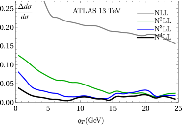
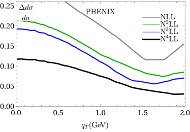
Figure 1: Ratio of scale variation band over theoretical cross section at different perturbative orders for Z/$\gamma$-boson production at ATLAS at $\sqrt{s}=13$ TeV (left), and for the DY process at PHENIX (right). The NP parameters and the PDF set are kept fixed. The definition of the variation band is given in eq. (37).

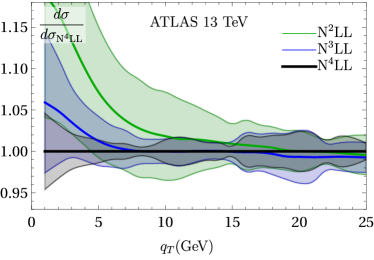
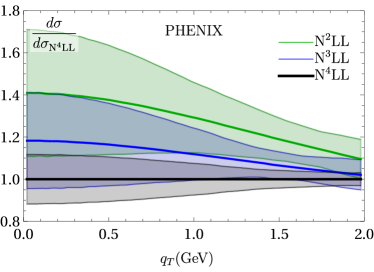
Figure 2: Ratio of cross sections at different orders over the one at N⁴LL with the corresponding scale-variation band for the kinematics of Z/$\gamma$-boson production at ATLAS at $\sqrt{s}=13$ TeV, and for DY process at PHENIX.

To define the scale-variation band we equip each scale by an independent factor $s_{i}$ ($i=2,3,4$), by the rule

$$\Big{\{}\mu\to s_{2}\mu,\mu^{*}\to s_{3}\mu^{*},\mu_{\text{OPE}}\to s_{4}\frac{2e^{-\gamma_{E}}}{b}+2\text{GeV}\Big{\}}.$$ (36)

The labels of parameters $s_{i}$ follow the enumeration used in ref. Landry:2002ix . The rule for $\mu_{\text{OPE}}$ is designed such that the variation of scale does not impact the NP large-$b$ part of the TMD distribution. As customary, each $s_{i}$ is allowed to vary by a factor 2, i.e. can take values $\{0.5,1,2\}$. In total, there are 27 combinations of $\{s_{2},s_{3},s_{4}\}$. For each one of them we compute the cross-section $d\sigma_{i}$. The size of the variation band is defined as the maximum (symmetric) deviation from the central value, i.e.

$$\Delta d\sigma=\max\left(|d\sigma_{i}-d\sigma|_{i=1...27}\right).$$ (37)

In fig. 1 we compare the sizes of variation bands for representatives of high and low energy experiments for four consecutive orders, while using the same values of the NP parameter and the same PDFs. In fig. 2 the same comparison is done for the absolute values of the cross-sections. As expected, we observe that the size of the bands reduces increasing the perturbative order. Each next-order curve is inside the variation band of the previous one. We also notice that for $q_{T}>5$ GeV the curves are close to each other. It indicates that convergence of the perturbative series is better than what one could estimate from the variation bands and that the rule in eq. (37) is too conservative.

For small values of transverse momentum ($q_{T}<5$ GeV), the dominant contribution to the variation band arises from the factor $s_{4}$. However, it is worth noticing that in this regime the scale variation band is still not significant, as the effects of non-perturbative parameters override those of the perturbation theory. For $q_{T}>5$ GeV, the variation band is largely determined by the variation of $s_{3}$, and in this range, it remains nearly constant. For the ATLAS experiment at $\sqrt{s}=13$ TeV, the mean value of the variation band for $5$ GeV $<q_{T}<25$ GeV is 1.3$\%$. At low energies, the variation band remains large (around 10$\%$) even at the N⁴LL level, but this is not a problem because in this range the theory prediction is largely non-perturbative.

We also note that the oscillations happen in the variation band at $q_{T}>10$ GeV. Studying this effect in detail, we have concluded that it is connected to our implementation of the flavor variable number mass scheme in a complex way. Basically, the discontinuities in the shapes of the distributions (due to the quark mass thresholds) change positions during varying parameters $s_{i}$. These discontinuities generate tiny oscillations in the cross-section. For a natural selection of scales (that minimizes logarithms), the discontinuities (and hence the oscillations) are negligible, but some combinations of $s_{i}$’s are especially oscillatory since they generate many discontinuities. Therefore, the final shapes in fig. 1 are generated by the overlapping of the 27 curves with small oscillations in each one. We will address this problem in future works.

2.6 Summary on theory input

The cross-section of the vector boson production is computed with eqs. (6) and (2.1), for neutral and charged EW boson, respectively. The structure function $W_{f_{1}f_{1}}$ is evaluated in the TMD factorization framework and given in eq. (2.2). The evolution of TMDPDFs is computed using the $\zeta$-prescription, and the phenomenological ansätze for the optimal unpolarized TMDPDFs and CS kernel are defined in eqs. (31) and (35). At small-$b$ the TMDPDFs are matched to the unpolarized PDFs, for which we use the MSHT20 extraction at NNLO  Bailey:2020ooq . In tab. 2 we list the perturbative orders used in each factor of the N⁴LL cross section. In total, there are 13 free parameters to be determined by the fitting procedure: 3 of these describe the CS kernel, while the remaining 10 are for the unpolarized TMDPDFs.

3 Overview of data

The factorization formulas, eqs. (6) and (2.1), are valid at small values of $q_{T}^{2}/Q^{2}$. This restriction has been studied from the phenomenological point of view in refs. Scimemi:2017etj ; Scimemi:2019cmh ; Bacchetta:2019sam . The common conclusion is that, for $q_{T}/Q<0.25$, the power corrections remain at the level of 1%, and therefore the data can be safely included in phenomenological extractions. Above this threshold, the deviation between the theory and the measurements grows. However, such a simplistic rule does not work for data with precision of the order (or better than) 1%. In this case, the power corrections significantly affect the quality of the description, despite being numerically small.

In this work, we use the same general strategy for selecting the data as in refs. Scimemi:2019cmh ; Bertone:2019nxa . Namely, we only include in our fit a data point if it fulfils the conditions

$$\frac{\langle q_{T}\rangle}{\langle Q\rangle}\equiv\delta<0.25\quad\text{ and }\quad\left(\delta^{2}<2\sigma\quad\text{or}\quad\langle q_{T}\rangle<10\text{ GeV}\right),$$ (38)

where $\langle q_{T}\rangle$ and $\langle Q\rangle$ are the average values of $q_{T}$ and $Q$ for the bin, and $\sigma$ is the relative uncorrelated uncertainty. The second condition is actually needed only for the high-energy data, as it is satisfied by all the data from the lower energy experiments with $Q<40$ GeV. The selection rules of eq. (38) allow us to keep control of the predictive power of the theory, and still incorporate a large amount of data into the fit procedure. They are slightly softer than the rules used in refs. Scimemi:2019cmh ; Bertone:2019nxa , because we plainly include all data with $\langle q_{T}\rangle<10\text{ GeV}$.

The bulk of the data considered here has already been used in previous extractions, such as Scimemi:2017etj ; Bertone:2019nxa ; Scimemi:2019cmh ; Bacchetta:2019sam ; Bacchetta:2022awv . This includes the fixed-target E288, E605, E772 experiments from FermiLab (263 data points) Ito:1980ev ; Moreno:1990sf ; E772:1994cpf , the Z-boson production data from the CDF and D0 experiments at Tevatron (107 data points) CDF:1999bpw ; CDF:2012brb ; D0:1999jba ; D0:2007lmg ; D0:2010dbl , and the LHC run-1 and run-2 measurements of Z-boson production by the ATLAS, CMS, and LHCb collaborations (75 data points) ATLAS:2015iiu ; CMS:2011wyd ; CMS:2016mwa ; LHCb:2015okr ; LHCb:2015mad . Since these datasets are well-known and have been well-studied in the past, we refer the reader to Scimemi:2017etj ; Scimemi:2019cmh ; Bacchetta:2019sam ; Bacchetta:2022awv for a detailed discussion on their properties. In addition to these, we have included the latest measurements done at RHIC PHENIX:2018dwt ; STAR:SX and the LHC ATLAS:2019zci ; CMS:2019raw ; CMS:2021oex ; LHCb:2021huf , and the W-boson production data from Tevatron CDF:1991pgi ; D0:1998thd . As we consider these data in the framework of TMD factorization for the first time, we find it worthwhile to highlight the particularities of each set in the following lines.

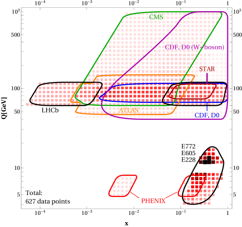
Figure 3: Distribution of data in the $(x,Q)$ plane. Each data point can span large regions. The color gradient darkens with an increasing number of data points contributing to a particular $(x,Q)$ point.

The PHENIX data PHENIX:2018dwt were taken at $\sqrt{s}=200$ GeV, which restricts the $Q$ range ($\langle Q\rangle=7$ GeV). It is the only modern DY measurement at low energy presently available, and has already been studied within TMD factorization in refs. Scimemi:2019cmh ; Bacchetta:2019sam ; Bacchetta:2022awv . The $Z/\gamma$-boson production measurement at STAR STAR:SX was made at moderately high energy ($\sqrt{s}=510$ GeV) during the 2018-2020 runs and the final results are currently in preparation for publication. Here we used the preliminary data.

In the present fit we include the recent $y$-differential measurements of Z-boson production at CMS CMS:2019raw and LHCb LHCb:2021huf , at $\sqrt{s}=13$ TeV. These replace the corresponding integrated measurements used in Scimemi:2019cmh . We also include the most precise ($\sim 0.1$% uncertainty) measurement of the Z-boson differential cross-section by ATLAS ATLAS:2019zci . Finally, we include the high-$Q$ neutral-boson production measurements by the CMS collaboration CMS:2021oex . This dataset is unique, since it spans up to $Q=1$ TeV (in several bins). For the interpretation of these data one should take into account that the bin-migration effects due to final state radiation are not incorporated in the published tables . Accounting for these effects is critical to confirm the agreement between theory and measurement. Moreover, we were not able to describe the lowest lying bin $50$ GeV$<Q<76$ GeV, for which we encountered a large difference in the normalization, and therefore, we exclude this bin. We have also excluded the $76$ GeV$<Q<106$ GeV bin, using instead the $y-$differential measurement from the same run CMS:2019raw .

For the first time in a TMD phenomenology, we include W-boson production data CDF:1991pgi ; D0:1998thd . Generally, the description of this observable is problematic within the TMD factorization framework because, ordinarily, the data are integrated over a wide kinematic range, including regions where the TMD factorization conditions are not fulfilled. For a detailed discussion of this issue, see Gutierrez-Reyes:2020ouu . While the measurements CDF:1991pgi ; D0:1998thd are fully integrated in $Q$, an explicit restriction on the transverse energy of the electron and neutrino (the missed transverse energy) was also imposed. This permits to find the lowest limit for $Q$. We have restricted the upper limit of integration to $300\,$GeV, since the contribution of higher $Q$ provides a negligible correction. To estimate the cut rules of eq. (38) for these data we used $\langle Q\rangle=M_{W}$.

In total, the present analysis includes 627 data points, summarized in tab. 3. The kinematical coverage of the datasets in the $(x,Q)$-plane is shown in fig. 3. All the new data (w.r.t. Bertone:2019nxa ; Scimemi:2019cmh ; Bacchetta:2019sam ) are at high energy. In fact, the new dataset totally supersedes the previous ones in both number of points (e.g. present fit includes 227 points from LHC, vs. 80 in Scimemi:2019cmh ) and precision. Therefore, the present selection allows for a more precise determination of the CS kernel (due to increased span in $Q$) and provides a finer flavor separation due to the W-boson measurements.

Experiment	ref.	$\sqrt{s}$ [GeV]	$Q$ [GeV]	$y$/$x_{F}$	fiducial region	$N_{\rm pt}$ after cuts
E288 (200)	Ito:1980ev	19.4	4 - 9 in 1 GeV bins∗	$0.1<x_{F}<0.7$	-	43
E288 (300)	Ito:1980ev	23.8	4 - 12 in 1 GeV bins∗	$-0.09<x_{F}<0.51$	-	53
E288 (400)	Ito:1980ev	27.4	5 - 14 in 1 GeV bins∗	$-0.27<x_{F}<0.33$	-	79
E605	Moreno:1990sf	38.8	7 - 18 in 5 bins∗	$-0.1<x_{F}<0.2$	-	53
E772	E772:1994cpf	38.8	5 - 15 in 8 bins∗	$0.1<x_{F}<0.3$	-	35
PHENIX	PHENIX:2018dwt	200	4.8 - 8.2	$1.2<y<2.2$	-	3
STAR	STAR:SX	510	73 - 114	$|y|<1$	$p_{T}>25$ GeV $|\eta|<1$	11
CDF (run1)	CDF:1999bpw	1800	66 - 116	-	-	33
CDF (run2)	CDF:2012brb	1960	66 - 116	-	-	45
CDF (W-boson)	CDF:1991pgi	1960	Q$>$40	-	$p_{T,e},p_{T,\nu}>20$GeV	6
D0 (run1)	D0:1999jba	1800	75 - 105	-	-	16
D0 (run2)	D0:2007lmg	1960	70 - 110	-	-	9
D0 (run2)μ	D0:2010dbl	1960	65 - 115	$|y|<1.7$	$p_{T}>15$ GeV $|\eta|<1.7$	4
D0 (W-boson)	D0:1998thd	1800	Q$>$50	-	$p_{T,e},p_{T,\nu}>25$GeV	7
ATLAS (8TeV)	ATLAS:2015iiu	8000	66 - 116	$|y|<2.4$ in 6 bins	$p_{T}>20$ GeV $|\eta|<2.4$	30
ATLAS (8TeV)	ATLAS:2015iiu	8000	46 - 66	$|y|<2.4$	$p_{T}>20$ GeV $|\eta|<2.4$	5
ATLAS (8TeV)	ATLAS:2015iiu	8000	116 - 150	$|y|<2.4$	$p_{T}>20$ GeV $|\eta|<2.4$	9
ATLAS (13TeV)	ATLAS:2019zci	13000	66 - 116	$|y|<2.5$	$p_{T}>27$ GeV $|\eta|<2.5$	5
CMS (7TeV)	CMS:2011wyd	7000	60 - 120	$|y|<2.1$	$p_{T}>20$ GeV $|\eta|<2.1$	8
CMS (8TeV)	CMS:2016mwa	8000	60 - 120	$|y|<2.1$	$p_{T}>20$ GeV $|\eta|<2.1$	8
CMS (13TeV)	CMS:2019raw	13000	76 - 106	$|y|<2.4$ in 5 bins	$p_{T}>25$ GeV $|\eta|<2.4$	64
CMS (13TeV)	CMS:2021oex	13000	106 - 170 170 - 350 350 - 1000	$|y|<2.4$	$p_{1T}>25$ GeV $p_{2T}>20$ GeV $|\eta|<2.4$	34
LHCb (7TeV)	LHCb:2015okr	7000	60 - 120	$2<y<4.5$	$p_{T}>20$ GeV $2<\eta<4.5$	8
LHCb (8TeV)	LHCb:2015mad	8000	60 - 120	$2<y<4.5$	$p_{T}>20$ GeV $2<\eta<4.5$	7
LHCb (13TeV)	LHCb:2021huf	13000	60 - 120	$2<y<4.5$ in 5 bins	$p_{T}>20$ GeV $2<\eta<4.5$	49
Total						627

*Bins with $9\lesssim Q\lesssim 11$ are omitted due to the $\Upsilon$ resonance.

Table 3: Summary table of the data included in the fit. For each dataset we report: the reference, the centre-of-mass energy, the coverage in $Q$ and $y/x_{F}$, the cuts on the fiducial region (if any), and the number of data points that survive the cut of eq. (38).

4 Fit procedure

Comparing the theory prediction with the data, we are able to restrict the free parameters of our ansatz for the TMD distributions, and in this way determine its NP component. This procedure is standard, and the present implementation is generally the same as the ones used in refs. Scimemi:2017etj ; Bertone:2019nxa ; Scimemi:2019cmh ; Bacchetta:2019sam ; Bacchetta:2022awv . However, in the present fit we treat the uncertainties more accurately and (for the first time) the PDF uncertainties are taken into account. The details of the procedure are reviewed in this section.

4.1 Treatment of the experimental data

In the measurement of the cross-sections in an experiment there are several features that should be treated accurately in order to achieve a better consistency. We point them out one-by-one below.

Bin integration. The expression for the cross-section in eq. (2.1) is given for a single point in the $(Q^{2},y,q_{T})$-space. On the experimental side, the measurement is provided for a volume-element of phase space, which can be obtained by averaging the theoretical expression

$$\frac{d\sigma}{dQ^{2}dyd\bm{q}_{T}^{2}}\Big{|}_{\text{exp}} = (Q^{2}_{\text{max}}-Q^{2}_{\text{min}})^{-1}(y_{\text{max}}-y_{\text{min}})^{-1}(\bm{q}_{T\text{max}}^{2}-\bm{q}^{2}_{T\text{min}})^{-1}$$

$$\qquad\times\int_{Q_{\text{max}}}^{Q_{\text{min}}}2QdQ\int_{y_{\text{max}}}^{y_{\text{min}}}dy\int_{q_{T\text{max}}}^{q_{T\text{min}}}2\bm{q}_{T}d\bm{q}_{T}\frac{d\sigma}{dQ^{2}dyd\bm{q}_{T}^{2}}\Big{|}_{\text{th.}}.$$

Here, the $Q_{\text{max}/\text{min}}$, $y_{\text{max}/\text{min}}$, and $\bm{q}_{T\text{max}/\text{min}}$ are the boundaries of the phase-space volume (bin). These integrations could not be simplified analytically, since the expression for the cross-section is too involved (especially in the presence of fiducial cuts). Accounting for the effect of finite bin size is of crucial importance, since for most of the experiments $d\sigma|_{\text{th.}}$ changes significantly and non-linearly within the bin. It should also be taken into account that some experiments provide integrated (rather than averaged) data. For example, the LHCb measurements in refs. LHCb:2015okr ; LHCb:2015mad are given for $\Delta\sigma$, that is, the bin integrated cross-section without any weighting factors.

Normalization. In a few cases the measurement is normalized to the total cross-section, i.e.

$$\frac{1}{\sigma}\frac{d\sigma}{dQ^{2}dyd\bm{q}_{T}^{2}}=\left(\int_{0}^{\infty}\frac{d\sigma}{dQ^{2}dyd\bm{q}_{T}^{2}}d\bm{q}_{T}^{2}\right)^{-1}\frac{d\sigma}{dQ^{2}dyd\bm{q}_{T}^{2}}.$$ (40)

This practice helps to reduce the normalization uncertainty of the measurement. Our formalism does not allow the computation of the weighting factor, since it includes the values of $q_{T}$ beyond the factorization range. In these cases we adopt the following procedure Scimemi:2017etj ; Bertone:2019nxa ; Scimemi:2019cmh . We compute

$$\frac{1}{\sigma}\frac{d\sigma}{dQ^{2}dyd\bm{q}_{T}^{2}}\simeq\mathcal{N}\frac{d\sigma}{dQ^{2}dyd\bm{q}_{T}^{2}},\qquad\mathcal{N}=\frac{\sum_{\begin{subarray}{c}\text{included}\\ \text{bins}\end{subarray}}\sigma^{-1}\frac{d\sigma}{dQ^{2}dyd\bm{q}_{T}^{2}}\Big{|}_{\text{exp.}}}{\sum_{\begin{subarray}{c}\text{included}\\ \text{bins}\end{subarray}}\frac{d\sigma}{dQ^{2}dyd\bm{q}_{T}^{2}}\Big{|}_{\text{th.}}},$$ (41)

i.e. we normalize to the area of included data points. Note, that the normalization is done after the bin-integration. This procedure reduces the amount of information which can be gained from the data; therefore, we use the absolute-value data whenever possible. Only the following datasets require a normalization factor: D0 (run2) D0:2007lmg ; D0:2010dbl , ATLAS (13 TeV) ATLAS:2019zci , and W-boson measurements CDF:1991pgi ; D0:1998thd .

Nuclear effects. The fixed target experiments are done on nuclear targets (Cu for E288 and E605 Ito:1980ev ; Moreno:1990sf , and $\,{}^{2}\!H$ for E772 E772:1994cpf ). To simulate the nuclear environment we perform the iso-spin rotation of the TMD distribution. Namely, we set

$$f_{1,u\leftarrow A}(x,b) = \frac{Z}{A}f_{1,u\leftarrow p}(x,b)+\frac{A-Z}{A}f_{1,d\leftarrow p}(x,b),$$ (42)

$$f_{1,d\leftarrow A}(x,b) = \frac{Z}{A}f_{1,d\leftarrow p}(x,b)+\frac{A-Z}{A}f_{1,u\leftarrow p}(x,b),$$

where $A$ is the atomic number and $Z$ is the charge of a nuclear target. The effects of heavier mass in the TMD distribution can be ignored since they are compensated by the scaling of the momentum fraction, as it has been shown in ref. Moos:2020wvd . We do not include any finer modifications, since the fixed target data are not precise enough to distinguish them.

Artemide. The computation of the theory prediction, as well as all integrals and factors required for comparison with the data, are done in artemide, a multi-purpose code for the phenomenology of TMD factorization. It is based on the $\zeta$-prescription, which allows for many simplifications of the code and improves the speed of the computation. In particular, the computation of the theory prediction for the full dataset (627 points) with all integrations required for comparison with experiment consumes 20-30 seconds on the average desktop (12 cores processor) depending on the NP input. The code of artemide is written in FORTRAN95. It is open-source and available at artemide . The values of $\alpha_{s}$ and the collinear PDFs are obtained from the LHAPDF interface Buckley:2014ana .

The legacy of artemide is established in many previous global fits, including fits of various unpolarized Scimemi:2017etj ; Bertone:2019nxa ; Vladimirov:2019bfa ; Scimemi:2019cmh ; Hautmann:2020cyp ; Gutierrez-Reyes:2020ouu ; Bury:2022czx , and polarized Bury:2020vhj ; Bury:2021sue ; Horstmann:2022xkk observables. For the present work we have updated it with the expressions for N³LO coefficient functions and N³LO anomalous dimensions, without further modifications of the internal structure of the code.

4.2 Definition of the $\chi^{2}$-test function and related quantities

The agreement of the theory prediction and the data is quantified by the $\chi^{2}$-test function. We use the standard definition adopted from the fits of collinear PDFs in refs. Ball:2008by ; Ball:2012wy , to which we refer the reader for a detailed discussion. The $\chi^{2}$-test function is defined as

$$\chi^{2}=\sum_{i,j\in\text{data}}(m_{i}-t_{i})V^{-1}_{ij}(m_{j}-t_{j}),$$ (43)

where $i$ and $j$ run over all data points included into the fit, $m_{i}$ and $t_{i}$ are the experimental value and theoretical prediction for point $i$, respectively, and $V^{-1}_{ij}$ is the inverse of the covariance matrix. The covariance matrix is defined as

$$V_{ij}=\delta_{ij}\Delta_{i,\text{uncorr}.}^{2}+\sum_{l}\Delta_{i,\text{corr}.}^{(l)}\Delta_{j,\text{corr}.}^{(l)},$$ (44)

where $\Delta_{i,\text{uncorr}.}$ is the uncorrelated uncertainty of the measurement (if there are more than one, they are summed in squares), and $\Delta_{i,\text{corr}.}^{(l)}$ is the $l$-th correlated uncertainty. The normalization uncertainty (due to the luminosity) is included in the $\chi^{2}$ as one of the correlated uncertainties. This definition of the covariance matrix and the $\chi^{2}$-test function takes into account the nature of the experimental uncertainties and also provides a faithful estimate of the agreement between data and theoretical predictions.

Additionally, this definition of $\chi^{2}$ allows for an one-to-one separation of correlated and uncorrelated parts Ball:2012wy for each correlated dataset. Therefore,

$$\chi^{2}=\chi^{2}_{D}+\chi^{2}_{\lambda},$$ (45)

where $\chi^{2}_{D}$ incorporates the contribution due to the uncorrelated uncertainties of the measurement, while $\chi^{2}_{\lambda}$ is the rest. The definitions of $\chi_{D}^{2}$ and $\chi_{\lambda}^{2}$ are

$$\chi_{D}^{2}=\sum_{i}\frac{(m_{i}-\bar{t}_{i})^{2}}{\Delta_{i,\text{uncorr.}}^{2}},\qquad\chi_{\lambda}^{2}=\sum_{l}\lambda_{l}^{2},$$ (46)

with $\lambda$ and $\bar{t}$ defined below. Loosely speaking, $\chi^{2}_{D}$ ($\chi^{2}_{\lambda}$) shows the agreement in the shape (normalization) between the theory prediction and the experimental measurement.

To perform this decomposition, one should compute the “nuisance parameters” $\lambda_{l}$ ($l$ enumerates the number of correlated uncertainties for the given dataset) Ball:2012wy ; Bertone:2019nxa for a given theory prediction. Then the theory prediction is decomposed as

$$t_{i}=\bar{t}_{i}-d_{i},\qquad d_{i}=\sum_{l}\lambda_{l}\Delta^{(l)}_{\text{corr.}}~{}.$$ (47)

The terms $d_{i}$ are interpreted as correlated shifts in the predictions which generate the $\chi^{2}_{\lambda}$ contribution. The terms $\bar{t}_{i}$ represent the part of the theory curve that contributes solely to $\chi^{2}_{D}$, and thus has a “perfect” normalization.

This decomposition is often useful for analysis and visualization because the correlated (normalization) uncertainty is generally much larger than the uncorrelated one. Hence, in plots comparing with data, we show the $\bar{t}_{i}$ part of the prediction. This allows us to visually confirm the “good” values of $\chi^{2}$. The average value of correlated shifts relative to the cross-section $\langle d_{i}/\sigma\rangle$ is presented in tab. 4. It exhibits the general disagreement in the normalization between the predictions of TMD factorization and the measurements.

The computation of the $\chi^{2}$ value and further manipulations are performed with the DataProcessor library, which is written in PYTHON and interfaced to artemide via the standard f2py library. The code of DataProcessor, together with the collection of the experimental data points, and all programs used for the present work, can be found in DataProcessor .

4.3 Minimisation procedure and uncertainty estimation

The ansatz for the TMD distributions contains in total 13 parameters, which we denote as $\overrightarrow{\lambda}$

$$\overrightarrow{\lambda}=\{B_{\text{NP}},c_{0},c_{1},\lambda_{1}^{u},\lambda_{2}^{u},\lambda_{1}^{d},\lambda_{2}^{d},\lambda_{1}^{\bar{u}},\lambda_{2}^{\bar{u}},\lambda_{1}^{\bar{d}},\lambda_{2}^{\bar{d}},\lambda_{1}^{sea},\lambda_{2}^{sea}\}.$$ (48)

To find the optimal values of $\overrightarrow{\lambda}$ we minimize the $\chi^{2}$ using the library iMinuit iminuit . The resulting value $\overrightarrow{\lambda}_{\text{center}}$ is called central value fit. The central value fit is used only as an initial assumption for all further minimization procedures described below.

The propagation of initial uncertainties to extracted values of the TMD distributions is both the central component and the most time-consuming step in the computation. We employ the resampling method to perform this task, generating samples of setups distributed according to the initial uncertainties. We distinguish two sources of uncertainties:

• Experimental uncertainties. These are uncertainties due to the imperfectness of the experimental measurements (statistical, systematic, etc.). To propagate these uncertainties we generate replicas of pseudo-data. A replica consisting of pseudo-data is obtained by adding Gaussian noise to the values of the data points. The parameters of the noise are dictated by the correlated and uncorrelated experimental uncertainties. Here, one should account for the nature of the correlated uncertainty in order to avoid the so-called D’Agostini bias DAgostini:2003syq . The detailed algorithm for the generation of pseudo-data is given in ref. Ball:2008by .

• Uncertainty in collinear PDFs. To propagate these uncertainties we use the Monte-Carlo sampling of the PDF distributions. The MSHT PDF set is given with (asymmetric) Hessian uncertainties, and the Monte-Carlo sample is generated according to the prescription given in ref. Hou:2016sho .

Other sources of uncertainties (such as uncertainties in $M_{Z}$ or $\alpha_{s}$, uncertainties due to missed higher perturbative orders, etc) are considered negligible.

The initial uncertainties included in the analysis originate from different sources, and it is not always clear how they should be combined. This is because the propagation mechanism for each uncertainty differs. The experimental uncertainties modify the expression of $\chi^{2}$ (by changing $V$ and $m$), while the PDF uncertainty changes the theory expression (by changing the boundary value of the TMD distribution). In this work, we consider them on the same foot and generate samples by varying data and PDF simultaneously. Here, the PDF replica is randomly selected from the pre-generated sample , and thus could be present in the final ensemble several times. Other possibilities are discussed in ref. Bury:2022czx .

For each setup sample, we minimize the $\chi^{2}$-function and find a set of parameters $\overrightarrow{\lambda}$, which defines the minimum. This procedure is repeated 1000 times, giving us an ensemble $\{\Lambda_{i}=(\overrightarrow{\lambda}_{i},n_{i})\}$, where $i=1,...,1000$ and $n_{i}$ is the serial number of PDF replica used in the sample setup. The PDF replica’s serial numbers must be preserved since the values of $\overrightarrow{\lambda}$ are essentially correlated with it. The ensemble of $\Lambda$’s entirely describes the TMD distributions and the CS kernel. This ensemble is used in all further manipulations. The list of values of $\Lambda_{i}$ can be found in the artemide repository artemide , in the (human-readable) format suitable for automatic processing by the DataProcessor.

Using the ensemble $\Lambda$, we can find the mean values of the parameters $\overrightarrow{\lambda}_{0}=\langle\overrightarrow{\lambda}_{i}\rangle$ associated with the central PDF replica (since the averaging of PDF replicas produces the central one by definition). The distribution is not entirely Gaussian, and this uncertainty band is associated with the $68\%$-confidence interval (68%CI). The boundaries of the 68%CI are computed using the resampling method by computing the 16% and 84% quantiles.

The central values and uncertainty bands for secondary values, such as TMD distributions, cross-sections, $\chi^{2}$, etc., are computed starting from the ensemble $\Lambda$. For example, to obtain the TMD distribution we compute the ensemble $F_{i}=F[\Lambda_{i}]$. The central value is then the mean $\langle F_{i}\rangle$ and the uncertainty band is 68%CI of $F_{i}$. Note, that $\langle F[\Lambda_{i}]\rangle\neq F[\langle\Lambda_{i}\rangle]$, due to the correlations in-between members of $\Lambda_{i}$. The procedure described above allows to propagate all correlations correctly.

This work presents a comprehensive analysis of error propagation in TMD phenomenology, which is the first of its kind. The proposed procedure is expected to reduce the dependence on PDFs as input parameters. However, the approach comes at the cost of increased computational complexity. In the present work, we use the MSHT20 PDF set Bailey:2020ooq , which we present as the main result. To cross check we also made an independent run (with 300 replicas) with the NNPDF3.1 PDF set NNPDF:2017mvq . The results of this run are given in the appendix A.

5 Results

In this section we present the results of the fitting procedure, starting with the quality of the data description, and finishing with the presentation of the extracted TMD distributions and CS kernel.

5.1 Quality of data description

We found that current setup perfectly describes the data. The central value fit results in $\chi^{2}/N_{\text{pt}}=0.93$. For the mean prediction (i.e. $\langle d\sigma[\Lambda_{i}]\rangle$), $\chi^{2}/N_{\text{pt}}=0.957$, with the 68%CI (0.950, 1.048). The histogram of $\chi^{2}/N_{\text{pt}}$ is given in fig. 4. The complete list of the $\chi^{2}$-values for all datasets is presented in tab. 4.

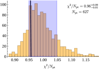
Figure 4: The histogram of the $\chi^{2}$ values for the full dataset. The black line marks the position of the mean prediction, and the blue band shows the 68%CI of the $\chi^{2}$ distribution.

dataset	$N_{\text{pt}}$	$\chi^{2}_{D}/N_{\text{pt}}$	$\chi^{2}_{\lambda}/N_{\text{pt}}$	$\chi^{2}/N_{\text{pt}}$	$\langle d/\sigma\rangle$
CDF (run1)	33	0.51	0.16	$0.67_{-0.03}^{+0.05}$	9.1%
CDF (run2)	45	1.58	0.11	$1.59_{-0.14}^{+0.26}$	4.0%
CDF (W-boson)	6	0.33	0.00	$0.33_{-0.01}^{+0.01}$	–
D0 (run1)	16	0.69	0.00	$0.69_{-0.03}^{+0.08}$	7.1%
D0 (run2)	13	2.16	0.16	$2.32_{-0.32}^{+0.40}$	–
D0 (W-boson)	7	2.39	0.00	$2.39_{-0.18}^{+0.20}$	–
ATLAS (8TeV, $Q\sim M_{Z}$)	30	1.60	0.49	$2.09_{-0.35}^{+1.09}$	4.1%
ATLAS (8TeV)	14	1.11	0.11	$1.22_{-0.21}^{+0.47}$	2.3%
ATLAS (13 TeV)	5	1.94	1.75	$3.70_{-2.24}^{+16.5}$	–
CMS (7TeV)	8	1.30	0.00	$1.30_{-0.01}^{+0.03}$	–
CMS (8TeV)	8	0.79	0.00	$0.78_{-0.01}^{+0.02}$	–
CMS (13 TeV, $Q\sim M_{Z}$)	64	0.63	0.24	$0.86_{-0.11}^{+0.23}$	4.3%
CMS (13 TeV, $Q>M_{Z}$)	33	0.73	0.12	$0.92_{-0.15}^{+0.40}$	1.0%
LHCb (7 TeV)	10	1.21	0.56	$1.77_{-0.31}^{+0.53}$	5.0%
LHCb (8 TeV)	9	0.77	0.78	$1.55_{-0.50}^{+0.94}$	4.3%
LHCb (13 TeV)	49	1.07	0.10	$1.18_{-0.01}^{+0.25}$	4.5%
PHENIX	3	0.29	0.12	$0.42_{-0.10}^{+0.15}$	10.%
STAR	11	1.91	0.28	$2.19_{-0.31}^{+0.51}$	15.%
E288 (200)	43	0.31	0.07	$0.38_{-0.05}^{+0.12}$	44.%
E288 (300)	53	0.36	0.07	$0.43_{-0.04}^{+0.08}$	48.%
E288 (400)	79	0.37	0.05	$0.48_{-0.03}^{+0.11}$	48.%
E772	35	0.87	0.21	$1.08_{-0.05}^{+0.08}$	27.%
E605	53	0.18	0.21	$0.39_{-0.00}^{+0.03}$	49.%
Total	627	0.79	0.17	$0.96_{-0.01}^{+0.09}$

Table 4: The values of $\chi^{2}$ for the individual datasets. The last column shows the average relative shifts computed by eqn.(47), which indicate the size of normalization discrepancy.

In comparison to the SV19 fit Scimemi:2019cmh we observe an overall improvement in the $\chi^{2}$, which is especially significant for the description of the LHC data ($\chi^{2}_{\text{LHC}}/N_{\text{pt}}=1.26_{-0.15}^{+0.76}$ with $N_{\text{pt}}=230$), and the low-energy DY data ($\chi^{2}_{\text{low}}/N_{\text{pt}}=0.50_{-0.03}^{+0.09}$ with $N_{\text{pt}}=266$). Similarly to SV19, we observe that the low-energy DY data suffer of deficits in the normalization. This is a known feature of TMD factorization (see e.g. the extended discussions in refs.Vladimirov:2019bfa ; Scimemi:2019cmh ). Given that the data have very large normalization uncertainties, these deficits do not significantly impact the value of $\chi^{2}$; therefore it is not clear at the moment, if the problem arises from a shortcoming of the theory or of the measurements. Let us also mention that the PHENIX measurement ($\langle Q\rangle=7$ GeV) does not show any problem with the normalization.

In fig. 5 we present the comparison of theory vs ATLAS 13 TeV measurement, which is the most precise measurement at our disposal (with uncorrelated uncertainties $<0.5\%$). In this plot one can see that TMD factorization works up to $q_{T}\simeq 0.2\ Q$ (even if in this particular case only data up to $q_{T}=10$ GeV were included into the fit). At larger $q_{T}$, the theory prediction is systematically lower than the measurement: this is a signal of the necessity for power corrections. The full collection of data plots is given in the appendix B.

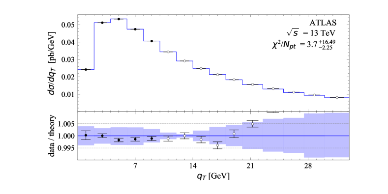
Figure 5: Comparison of data (here, the Z-Boson production at ATLAS $\sqrt{s}=13$ TeV measurement ATLAS:2019zci ) with the theoretical prediction. The blue band is the 68%CI. The filled points were included into the fit and the displayed $\chi^{2}$ corresponds to those only.

We emphasize that the uncertainty band obtained in this fit is larger than in our previous analysis. This is due to the inclusion of the PDF uncertainty. Also, since we cannot control the PDF uncertainty, the band is often larger than the uncertainty of the measurement. It indicates that a simultaneous extraction of PDF and TMD distributions will reduce the uncertainties of both. We also have observed that most part of our uncertainty band is correlated. To determine the size of the correlation we computed the covariance matrix for the full set of replicas, $\text{cov}(d\sigma(\Lambda_{i}),d\sigma(\Lambda_{j}))$ and fitted it with the form of eq. (44), and determined $\Delta_{\text{th.uncorr}}$ and $\Delta_{\text{th.corr}}$ for the theory prediction. We found that the portions of correlated and uncorrelated parts depend on $x$. Generally, the higher the value of $x$ the larger the uncorrelated part of the band. For example, for the Z-boson production at $\sqrt{s}=13$ TeV $\langle\Delta_{\text{th.uncorr}}\rangle\simeq 8.5\%$ at $|y|<0.4$, $\langle\Delta_{\text{th.uncorr}}\rangle\simeq 15\%$ at $2.0<y<2.4$, and $\langle\Delta_{\text{th.uncorr}}\rangle\simeq 48\%$ at $4<|y|<4.5$.

5.2 Collins-Soper kernel

The plot of the CS kernel is presented in fig. 6. The values of parameters that we obtain are

$$B_{\text{NP}}=1.56^{+0.13}_{-0.09}\text{GeV},\qquad c_{0}=3.69^{+0.65}_{-0.61}\cdot 10^{-2},\qquad c_{1}=5.82^{+0.64}_{-0.88}\cdot 10^{-2}.$$ (49)

The parameters $B_{\text{NP}}$ and $c_{0}$ are compatible with the ones extracted in SV19. In particular, for the MMHT14 PDF (predecessor of MSHT20) SV19 found $B_{\text{NP}}=1.55\pm 0.29$ and $c_{0}=(4.7\pm 1.47)\cdot 10^{-2}$. Nonetheless, the shape of the distributions changes significantly due to the new logarithmic term $\sim c_{1}$ in the ansatz of eq. (35). This term modifies the shape of the distribution at $b\sim 1-3$ GeV, leaving the large-$b$ asymptotic behaviour untouched. The general shape and value of the CS kernel are in good agreement with the MAP22 determination, as can be seen in fig. 6.

Of greater significance, in the current fit, the size of the uncertainty band for the CS kernel is reduced, in contrast to that of the TMD distribution itself. This is correct, since in the $\zeta$-prescription the CS kernel is exactly decorrelated from the TMDPDF (on the theory side), and the quality of the data has increased. We also notice that the parameter $c_{1}$ is clearly non-zero, which indicates the presence of a non-negligible logarithmic behaviour in the next-to-leading power term of the small-$b$ expansion of the CS kernel.

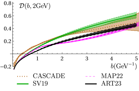
Figure 6: Plot of the Collins-Soper kernel at $\mu=2$ GeV. Different lines correspond to the independent extractions CASCADE BermudezMartinez:2022ctj , SV19 Scimemi:2019cmh , MAP22 Bacchetta:2022awv , and ART23 (this work).

5.3 Unpolarized TMD distribution

The values of the TMDPDF parameters extracted in the fit are

$$\lambda_{1}^{u}=0.87_{-0.10}^{+0.10}, \lambda_{2}^{u}=0.91_{-0.29}^{+0.33},$$ (50)

$$\lambda_{1}^{d}=0.99_{-0.12}^{+0.09}, \lambda_{2}^{d}=6.06_{-1.34}^{+1.36},$$

$$\lambda_{1}^{\bar{u}}=0.35_{-0.22}^{+0.23}, \lambda_{2}^{\bar{u}}=46.6_{-8.1}^{+7.9},$$

$$\lambda_{1}^{\bar{d}}=0.12_{-0.11}^{+0.13}, \lambda_{2}^{\bar{d}}=1.53_{-0.17}^{+0.54},$$

$$\lambda_{1}^{sea}=1.32_{-0.24}^{+0.23}, \lambda_{2}^{sea}=0.46_{-0.45}^{+0.13},$$

Most of these parameters have reasonable sizes, and they agree (within uncertainty) with similar ones found in ref. Bury:2022czx . However, the parameters $\lambda_{1}^{\bar{d}}$ and $\lambda_{2}^{sea}$ show some problematic behaviour. Namely, they almost vanish at their lower boundary. For negligible values of $\lambda$’s the $b-$profile of the corresponding TMDPDF flattens. This is a clearly non-physical behavior, which results in disturbed shapes of the uncertainty bands for $\bar{d}$ and $sea$ flavors at large-$b$. Simultaneously, it does not produce any problem in the prediction for the cross-section, since the TMDPDFs contributes in products with the evolution factors. It merely indicates that the present observables/data are not restrictive enough for these flavor combinations.

The shapes of the TMDPDFs are shown in fig. 7 for $u$ and $d$ quarks (other flavors show similar behaviour). The sizes of the uncertainty bands are shown in fig. 8 in comparison to the SV19 bands. Generally, the uncertainty bands are increased by an order of magnitude, and grow faster with the increase of $b$. This is the result of incorporating the PDF uncertainties, which helps to avoid the PDF-bias and allows for a more realistic uncertainty estimation. The $x$-shape of the uncertainties has become more involved. Their minimum is at $x\sim 10^{-2}$, where the most precise data are located. The sizes of quark- and anti-quark uncertainties are compatible, because most part of the data depend on the product $f_{1q}f_{1\bar{q}}$ that does not distinguish between quarks and anti-quarks.

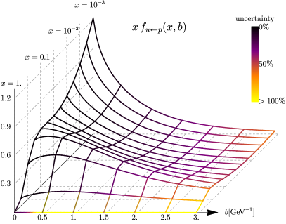
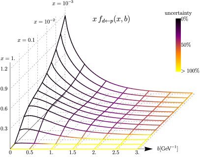
Figure 7: Shape of TMDs in the (x,b)-space. The color indicates the uncertainty.

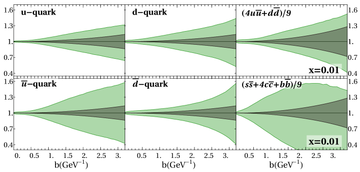
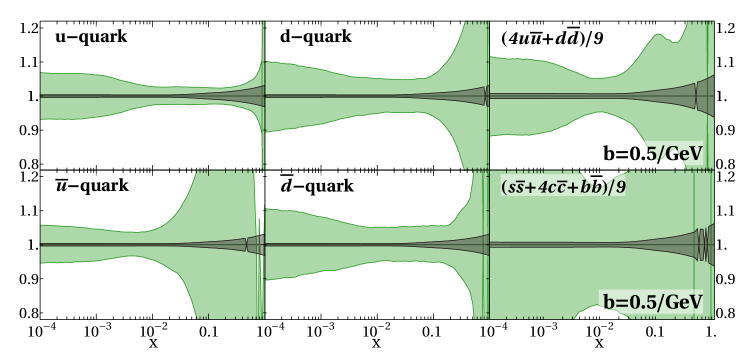
Figure 8: Sizes of the uncertainty bands in ART23 (green) in comparison to the those of the SV19 extraction (grey). The upper panel shows the $b$-dependence at $x=0.01$. The lower panel shows the $x-$dependence at $b=0.5$ GeV^-1.

6 Conclusions

The present extraction of unpolarized TMDPDF from the global fit of Drell-Yan data (refereed as ART23) represents a significant step forward in comparison to previous analyses. The main improvements are a higher order perturbative input (which reach N⁴LL), a consistent treatment of PDF uncertainties in the error analysis, and the inclusion of additional data. We also use the flavor dependent form of the fitting ansatz for TMDPDF. The introduction of flavor dependence reduces the sensitivity to the choice of PDF sets, as observed in Bury:2022czx . Furthermore, the newly incorporated non-perturbative logarithmic dependence of the Collins-Soper evolution kernel, eq. (35), plays a crucial role in achieving a successful fit.

We also find it particularly interesting that several groups find a reasonable agreement on the Collins-Soper kernel (see fig. 6) despite somewhat different functional forms and uncertainty-estimation procedure. Also the agreement with new Z-boson data at LHC and W-boson mediated data at Tevatron is particularly comforting.

It is important to stress that the PDF uncertainties dominate the TMDPDF extraction, see fig. 8. For that reason, the uncertianties on TMDPDFs that we find are larger by almost an order of magnitude in comparison to other global extractions Scimemi:2019cmh ; Bertone:2019nxa ; Bacchetta:2019sam ; Bacchetta:2022awv , even though the present dataset is about 30-40% larger and more precise than those considered earlier. We argue that this increased uncertainty is more realistic, and previous studies were biased in several aspects. The $\chi^{2}$ value that we obtain is very stable, see fig. 4, and it shows a very good agreement between the theory and the data. This observation is noteworthy and suggests that future improvements to the TMDPDFs determination could be achieved by a joint fit of PDFs and TMDPDFs. These possibilities will be explored in due time along with the inclusion of new data.

The values of ART23 unpolarized TMDPDFs, as well as, the artemide code release used for their extraction is published in the artemide-repository artemide . The accompanying code (for minimisation, generation of plots, etc) is presented in ref. DataProcessor . We also release ART23 TMDPFs in the unified format of TMDlib2 Abdulov:2021ivr .

Our current understanding of the TMDPDFs is summarized in fig. 7, which illustrates the shape and the uncertainty of the unpolarized TMD distributions in the $(x,b)$ plane for up and down quarks. An important point for future consideration is the impact of power corrections, for which preliminary theoretical results have been obtained but are not yet directly applicable to our present analysis Moos:2020wvd ; Ebert:2021jhy ; Rodini:2022wki .

Appendix A Fit using NNPDF3.1

In the present approach the TMDPDF suffers the PDF-bias Bury:2022czx , i.e. is strongly dependent on the collinear PDF. To explore this dependence, we have performed an additional fit using the NNPDF3.1 collinear PDF NNPDF:2017mvq with identically the same technique as presented in the main text. In this appendix we discuss the outcomes for the fit.

The fit procedure is described in sec. 4.3. In this fit we utilize the 1000-replica distribution of NNPDF3.1, and computed 300 replicas in total. The quality of the fit with NNPDF3.1 is worse, we obtain $\chi^{2}/N_{\text{pt}}=1.18^{+0.11}_{-0.05}$. The resulting values of parameters for the CS kernel are:

$$B_{\text{NP}}=1.82^{+0.37}_{-0.29}\text{ GeV},\qquad c_{0}=5.03^{+1.02}_{-0.81}\cdot 10^{-2},\qquad c_{1}=1.04^{+0.09}_{-0.15}\cdot 10^{-1}.$$ (51)

These parameters are quite different from the MSHT values (49). The comparison of the resulting CS kernels is given in fig. 9. In particular, we observe that the value of $B_{\text{NP}}$ has very large uncertanties, in contrast to the MSHT case.

Figure 9: Comparison of the CS kernels extracted with the MSHT20 (solid grey curve) and NNPDF3.1 (dashed orange curve) collinear PDFs.

The parameters of the TMD distribution’s ansatz are

$$\lambda_{1}^{u}=1.11_{-0.17}^{+0.15}, \lambda_{2}^{u}=2.69_{-2.53}^{+1.79},$$ (52)

$$\lambda_{1}^{d}=0.99_{-0.17}^{+0.14}, \lambda_{2}^{d}=3.60_{-3.57}^{+4.36},$$

$$\lambda_{1}^{\bar{u}}=0.37_{-0.15}^{+0.16}, \lambda_{2}^{\bar{u}}=75.0_{-13.2}^{+14.8},$$

$$\lambda_{1}^{\bar{d}}=0.37_{-0.32}^{+0.30}, \lambda_{2}^{\bar{d}}=17.7_{-14.2}^{+6.91},$$

$$\lambda_{1}^{sea}=1.88_{-0.29}^{+0.34}, \lambda_{2}^{sea}=2.71_{-2.69}^{+2.44}.$$

Generally, we observe that the NNPDF3.1-fit yields a different spread in the parameters with a larger uncertainty. Most of the parameters are in a relative agreement, however, the parameters $\lambda_{2}^{u}$, $\lambda_{2}^{\bar{u}}$, $\lambda_{2}^{\bar{d}}$ and $\lambda_{2}^{sea}$ disagree, and do not overlap within uncertainty bands. All these parameters are responsible for the behaviour of the TMDPDF at large-$x$, i.e. exactly in the region where collinear distributions differ. However, for the middle-$x$ range ($x\sim 10^{-2}-10^{-3}$) the TMDPDFs are in general agreement, except for the sea-quark (see fig. 10).

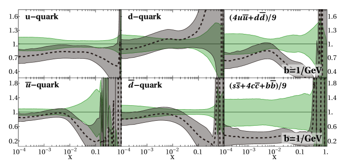
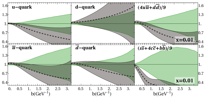
Figure 10: Comparison of uncertainty bands for unpolarized TMDPDFs extracted with MSHT20 (green) and NNPDF3.1 (gray) collinear distributions. The plots are normalized to the MSHT20 case.

The comparison of resulting theory predictions are given in fig. 11, for several bins of ATLAS at $\sqrt{s}=8$ TeV, and LHCb at $\sqrt{s}=13$ TeV. Other experiments demonstrate a similar picture. Comparing these two experiments one can see that both PDFs produce very similar results for ATLAS (which has $x\sim 10^{-2}-10^{-3}$, while for LHCb (which has $x\sim 10^{-1}$) the curves are very different. It confirms our previous conclusion that the extractions of TMDPDFs are very sensitive to the large-$x$ range.

Let us stress that without the inclusion of the flavor-dependence the extractions with MSHT20 and NNPDF3.1 diagree drastically Bury:2022czx . The inclusion of the flavor-dependence reduces the problem of the PDF-bias, but does not resolve it completely.

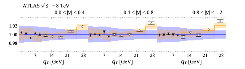
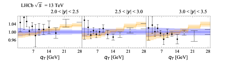
Figure 11: Comparison of theory predictions based on MHST20 (blue) or NNPDF3.1 (orange) collinear PDFs. The rapidity range is indicated above the plot. All data and uncertainties are normalized to the blue line (MSHT20 result).

Appendix B Comparison with data

In this appendix, we present all the data used for the fit, along with the resulting theory prediction of our main fit (with MSHT20 PDF input). The depicted theory prediction is the distributions (of replicas) average. The 68%CI of the theory prediction (see description in sec. 4.3) is shown as a blue band. For a better visual comparison of data and theory predictions, the theory curves are shifted by a factor $d$ (eq. (47)) computed for the central line of the prediction. In all plots, we demonstrate more data than those described by the TMD factorization theorem. The data points used in the fit are shown by filled points, while the rest are shown by empty points.

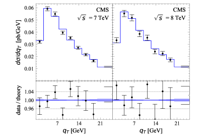
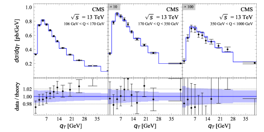
Figure 12: Differential cross-section for the $Z/\gamma^{*}$ boson production measured by CMS, at different values of $\sqrt{s}$ and $Q$, according to the legends in the plots.

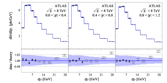
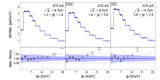
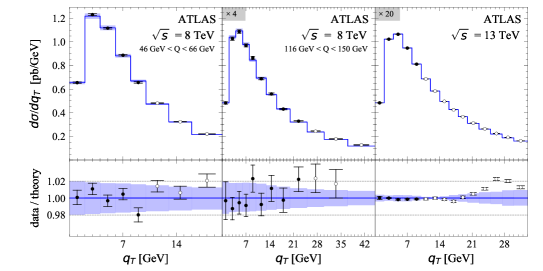
Figure 13: Differential cross-section for the $Z/\gamma^{*}$ boson production measured by ATLAS, at different values of $\sqrt{s}$, $y$, and $Q$. All details pertaining the values of the kinematic variables and their cut can be seen in the plots. The plot for comparison with ATLAS at $\sqrt{s}=13$ TeV can be found in fig.5 in a larger scale.

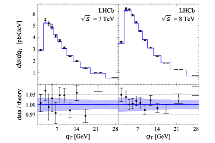
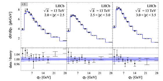
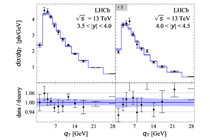
Figure 14: Differential cross-section for the $Z/\gamma^{*}$ boson production measured by LHCb, at different values of $\sqrt{s}$ and $y$, according to the legends in the plots.

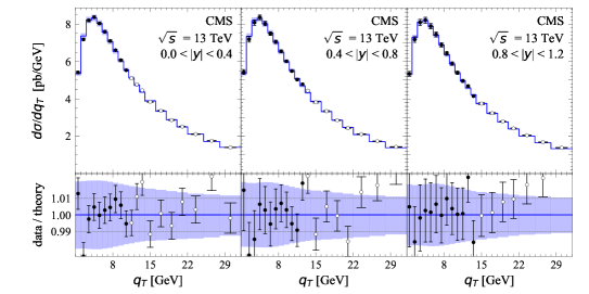
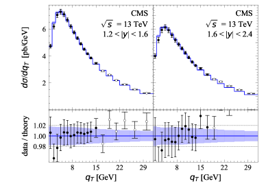
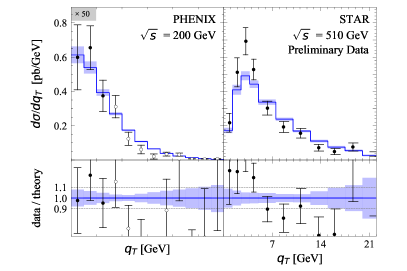
Figure 15: Upper and central rows: differential cross-section of the $Z/\gamma^{*}$ boson production measured by CMS at different values of $y$ (see the text on the plots for details). Lower row: differential cross-section for the DY process measured at PHENIX (left) and STAR (right).

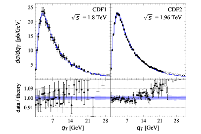
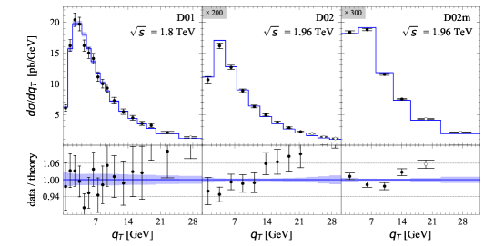
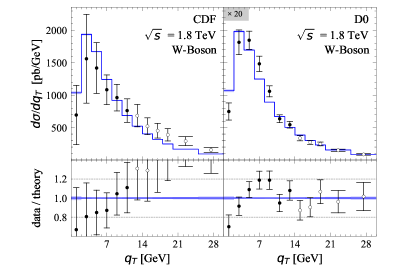
Figure 16: Differential cross-section for the $Z/\gamma^{*}$ (upper and center rows) and $W$ (lower row) boson production in the DY-process measured by CDF and D0, at different values of $\sqrt{s}$.

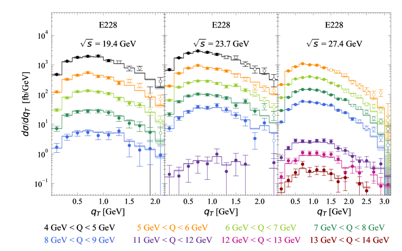
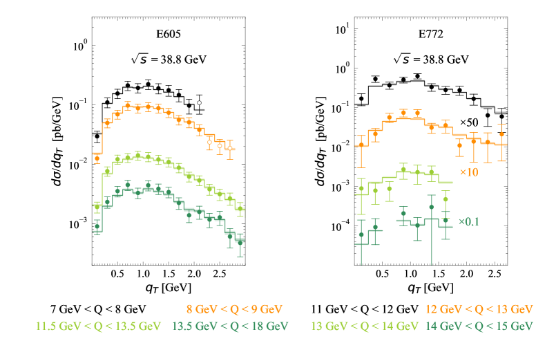
Figure 17: Differential cross section of the DY process measured by the E228, E605 and E772 experiments at different values of $\sqrt{s}$ and $Q$. To increase visibility, the data in different $Q-$bins of the E772 experiment are multiplied by the factors indicated in the plot.

References

- (1) T. Becher and M. Neubert, Drell-Yan Production at Small , Transverse Parton Distributions and the Collinear Anomaly, Eur. Phys. J. C 71 (2011) 1665 [1007.4005].
- (2) J. Collins, Foundations of perturbative QCD, vol. 32, Cambridge University Press (11, 2013).
- (3) M.G. Echevarria, A. Idilbi and I. Scimemi, Factorization Theorem For Drell-Yan At Low And Transverse Momentum Distributions On-The-Light-Cone, JHEP 07 (2012) 002 [1111.4996].
- (4) M.G. Echevarría, A. Idilbi and I. Scimemi, Soft and Collinear Factorization and Transverse Momentum Dependent Parton Distribution Functions, Phys. Lett. B 726 (2013) 795 [1211.1947].
- (5) I. Scimemi and A. Vladimirov, Analysis of vector boson production within TMD factorization, Eur. Phys. J. C 78 (2018) 89 [1706.01473].
- (6) A. Bacchetta, V. Bertone, C. Bissolotti, G. Bozzi, F. Delcarro, F. Piacenza et al., Transverse-momentum-dependent parton distributions up to N3LL from Drell-Yan data, JHEP 07 (2020) 117 [1912.07550].
- (7) V. Bertone, I. Scimemi and A. Vladimirov, Extraction of unpolarized quark transverse momentum dependent parton distributions from Drell-Yan/Z-boson production, JHEP 06 (2019) 028 [1902.08474].
- (8) I. Scimemi and A. Vladimirov, Non-perturbative structure of semi-inclusive deep-inelastic and Drell-Yan scattering at small transverse momentum, JHEP 06 (2020) 137 [1912.06532].
- (9) A. Bacchetta, V. Bertone, C. Bissolotti, G. Bozzi, M. Cerutti, F. Piacenza et al., Unpolarized Transverse Momentum Distributions from a global fit of Drell-Yan and Semi-Inclusive Deep-Inelastic Scattering data, 2206.07598.
- (10) T. Gehrmann, T. Lubbert and L.L. Yang, Transverse parton distribution functions at next-to-next-to-leading order: the quark-to-quark case, Phys. Rev. Lett. 109 (2012) 242003 [1209.0682].
- (11) T. Gehrmann, T. Luebbert and L.L. Yang, Calculation of the transverse parton distribution functions at next-to-next-to-leading order, JHEP 06 (2014) 155 [1403.6451].
- (12) M.G. Echevarria, I. Scimemi and A. Vladimirov, Universal transverse momentum dependent soft function at NNLO, Phys. Rev. D 93 (2016) 054004 [1511.05590].
- (13) M.G. Echevarria, I. Scimemi and A. Vladimirov, Unpolarized Transverse Momentum Dependent Parton Distribution and Fragmentation Functions at next-to-next-to-leading order, JHEP 09 (2016) 004 [1604.07869].
- (14) A.A. Vladimirov, Correspondence between Soft and Rapidity Anomalous Dimensions, Phys. Rev. Lett. 118 (2017) 062001 [1610.05791].
- (15) Y. Li and H.X. Zhu, Bootstrapping Rapidity Anomalous Dimensions for Transverse-Momentum Resummation, Phys. Rev. Lett. 118 (2017) 022004 [1604.01404].
- (16) ATLAS collaboration, Measurement of the transverse momentum distribution of Drell–Yan lepton pairs in proton–proton collisions at TeV with the ATLAS detector, Eur. Phys. J. C 80 (2020) 616 [1912.02844].
- (17) G. Das, S.-O. Moch and A. Vogt, Soft corrections to inclusive deep-inelastic scattering at four loops and beyond, JHEP 03 (2020) 116 [1912.12920].
- (18) M.-x. Luo, T.-Z. Yang, H.X. Zhu and Y.J. Zhu, Quark Transverse Parton Distribution at the Next-to-Next-to-Next-to-Leading Order, Phys. Rev. Lett. 124 (2020) 092001 [1912.05778].
- (19) A. von Manteuffel, E. Panzer and R.M. Schabinger, Cusp and collinear anomalous dimensions in four-loop QCD from form factors, Phys. Rev. Lett. 124 (2020) 162001 [2002.04617].
- (20) C. Duhr, F. Dulat and B. Mistlberger, Drell-Yan Cross Section to Third Order in the Strong Coupling Constant, Phys. Rev. Lett. 125 (2020) 172001 [2001.07717].
- (21) M.A. Ebert, B. Mistlberger and G. Vita, Transverse momentum dependent PDFs at N3LO, JHEP 09 (2020) 146 [2006.05329].
- (22) S. Moch, B. Ruijl, T. Ueda, J.A.M. Vermaseren and A. Vogt, Low moments of the four-loop splitting functions in QCD, Phys. Lett. B 825 (2022) 136853 [2111.15561].
- (23) L. Chen, M. Czakon and M. Niggetiedt, The complete singlet contribution to the massless quark form factor at three loops in QCD, JHEP 12 (2021) 095 [2109.01917].
- (24) C. Duhr, B. Mistlberger and G. Vita, Four-Loop Rapidity Anomalous Dimension and Event Shapes to Fourth Logarithmic Order, Phys. Rev. Lett. 129 (2022) 162001 [2205.02242].
- (25) I. Moult, H.X. Zhu and Y.J. Zhu, The four loop QCD rapidity anomalous dimension, JHEP 08 (2022) 280 [2205.02249].
- (26) M. Bury, F. Hautmann, S. Leal-Gomez, I. Scimemi, A. Vladimirov and P. Zurita, PDF bias and flavor dependence in TMD distributions, JHEP 10 (2022) 118 [2201.07114].
- (27) A. Vladimirov, Pion-induced Drell-Yan processes within TMD factorization, JHEP 10 (2019) 090 [1907.10356].
- (28) S. Fazio and X. Chu. private communication.
- (29) CMS collaboration, Measurements of differential Z boson production cross sections in proton-proton collisions at = 13 TeV, JHEP 12 (2019) 061 [1909.04133].
- (30) CMS collaboration, Measurement of mass dependence of the transverse momentum of Drell Yan lepton pairs in proton-proton collisions at , .
- (31) LHCb collaboration, Precision measurement of forward boson production in proton-proton collisions at TeV, JHEP 07 (2022) 026 [2112.07458].
- (32) CDF collaboration, Measurement of the W P(T) distribution in collisions at TeV, Phys. Rev. Lett. 66 (1991) 2951.
- (33) D0 collaboration, Measurement of the shape of the transverse momentum distribution of bosons produced in collisions at TeV, Phys. Rev. Lett. 80 (1998) 5498 [hep-ex/9803003].
- (34) S. Bailey, T. Cridge, L.A. Harland-Lang, A.D. Martin and R.S. Thorne, Parton distributions from LHC, HERA, Tevatron and fixed target data: MSHT20 PDFs, Eur. Phys. J. C 81 (2021) 341 [2012.04684].
-
(35)
“artemide.” stable version:
https://github.com/VladimirovAlexey/artemide-public
in-production version: https://github.com/VladimirovAlexey/artemide-development. - (36) NNPDF collaboration, Parton distributions from high-precision collider data, Eur. Phys. J. C 77 (2017) 663 [1706.00428].
- (37) J.-Y. Chiu, A. Jain, D. Neill and I.Z. Rothstein, A Formalism for the Systematic Treatment of Rapidity Logarithms in Quantum Field Theory, JHEP 05 (2012) 084 [1202.0814].
- (38) I. Scimemi and A. Vladimirov, Systematic analysis of double-scale evolution, JHEP 08 (2018) 003 [1803.11089].
- (39) J.C. Collins, D.E. Soper and G.F. Sterman, Factorization of Hard Processes in QCD, Adv. Ser. Direct. High Energy Phys. 5 (1989) 1 [hep-ph/0409313].
- (40) A. Vladimirov, Structure of rapidity divergences in multi-parton scattering soft factors, JHEP 04 (2018) 045 [1707.07606].
- (41) A. Vladimirov, V. Moos and I. Scimemi, Transverse momentum dependent operator expansion at next-to-leading power, 2109.09771.
- (42) D. Gutierrez-Reyes, S. Leal-Gomez and I. Scimemi, W-boson production in TMD factorization, Eur. Phys. J. C 81 (2021) 418 [2011.05351].
- (43) Particle Data Group collaboration, Review of Particle Physics, PTEP 2022 (2022) 083C01.
- (44) I. Balitsky and A. Tarasov, Power corrections to TMD factorization for Z-boson production, JHEP 05 (2018) 150 [1712.09389].
- (45) J.C. Collins and D.E. Soper, Back-To-Back Jets: Fourier Transform from B to K-Transverse, Nucl. Phys. B 197 (1982) 446.
- (46) F. Herzog, S. Moch, B. Ruijl, T. Ueda, J.A.M. Vermaseren and A. Vogt, Five-loop contributions to low-N non-singlet anomalous dimensions in QCD, Phys. Lett. B 790 (2019) 436 [1812.11818].
- (47) R.N. Lee, A. von Manteuffel, R.M. Schabinger, A.V. Smirnov, V.A. Smirnov and M. Steinhauser, Quark and Gluon Form Factors in Four-Loop QCD, Phys. Rev. Lett. 128 (2022) 212002 [2202.04660].
- (48) M.-x. Luo, T.-Z. Yang, H.X. Zhu and Y.J. Zhu, Unpolarized quark and gluon TMD PDFs and FFs at N3LO, JHEP 06 (2021) 115 [2012.03256].
- (49) S. Moch, J.A.M. Vermaseren and A. Vogt, The Three loop splitting functions in QCD: The Nonsinglet case, Nucl. Phys. B 688 (2004) 101 [hep-ph/0403192].
- (50) A.A. Vladimirov, Self-contained definition of the Collins-Soper kernel, Phys. Rev. Lett. 125 (2020) 192002 [2003.02288].
- (51) V. Moos and A. Vladimirov, Calculation of transverse momentum dependent distributions beyond the leading power, JHEP 12 (2020) 145 [2008.01744].
- (52) M.G. Echevarria, A. Idilbi, A. Schäfer and I. Scimemi, Model-Independent Evolution of Transverse Momentum Dependent Distribution Functions (TMDs) at NNLL, Eur. Phys. J. C 73 (2013) 2636 [1208.1281].
- (53) F. Herzog, B. Ruijl, T. Ueda, J.A.M. Vermaseren and A. Vogt, The five-loop beta function of Yang-Mills theory with fermions, JHEP 02 (2017) 090 [1701.01404].
- (54) T. Neumann and J. Campbell, Fiducial Drell-Yan production at the LHC improved by transverse-momentum resummation at N4LLp+N3LO, Phys. Rev. D 107 (2023) L011506 [2207.07056].
- (55) F. Landry, R. Brock, P.M. Nadolsky and C.P. Yuan, Tevatron Run-1 boson data and Collins-Soper-Sterman resummation formalism, Phys. Rev. D 67 (2003) 073016 [hep-ph/0212159].
- (56) A.S. Ito et al., Measurement of the Continuum of Dimuons Produced in High-Energy Proton - Nucleus Collisions, Phys. Rev. D 23 (1981) 604.
- (57) G. Moreno et al., Dimuon production in proton - copper collisions at = 38.8-GeV, Phys. Rev. D 43 (1991) 2815.
- (58) E772 collaboration, Cross-sections for the production of high mass muon pairs from 800-GeV proton bombardment of H-2, Phys. Rev. D 50 (1994) 3038.
- (59) CDF collaboration, The transverse momentum and total cross section of pairs in the boson region from collisions at TeV, Phys. Rev. Lett. 84 (2000) 845 [hep-ex/0001021].
- (60) CDF collaboration, Transverse momentum cross section of pairs in the -boson region from collisions at TeV, Phys. Rev. D 86 (2012) 052010 [1207.7138].
- (61) D0 collaboration, Measurement of the inclusive differential cross section for bosons as a function of transverse momentum in collisions at TeV, Phys. Rev. D 61 (2000) 032004 [hep-ex/9907009].
- (62) D0 collaboration, Measurement of the shape of the boson transverse momentum distribution in events produced at =1.96-TeV, Phys. Rev. Lett. 100 (2008) 102002 [0712.0803].
- (63) D0 collaboration, Measurement of the Normalized Transverse Momentum Distribution in Collisions at TeV, Phys. Lett. B 693 (2010) 522 [1006.0618].
- (64) ATLAS collaboration, Measurement of the transverse momentum and distributions of Drell–Yan lepton pairs in proton–proton collisions at TeV with the ATLAS detector, Eur. Phys. J. C 76 (2016) 291 [1512.02192].
- (65) CMS collaboration, Measurement of the Rapidity and Transverse Momentum Distributions of Bosons in Collisions at TeV, Phys. Rev. D 85 (2012) 032002 [1110.4973].
- (66) CMS collaboration, Measurement of the transverse momentum spectra of weak vector bosons produced in proton-proton collisions at TeV, JHEP 02 (2017) 096 [1606.05864].
- (67) LHCb collaboration, Measurement of the forward boson production cross-section in collisions at TeV, JHEP 08 (2015) 039 [1505.07024].
- (68) LHCb collaboration, Measurement of forward W and Z boson production in collisions at TeV, JHEP 01 (2016) 155 [1511.08039].
- (69) PHENIX collaboration, Measurements of pairs from open heavy flavor and Drell-Yan in collisions at GeV, Phys. Rev. D 99 (2019) 072003 [1805.02448].
- (70) A. Buckley, J. Ferrando, S. Lloyd, K. Nordström, B. Page, M. Rüfenacht et al., LHAPDF6: parton density access in the LHC precision era, Eur. Phys. J. C 75 (2015) 132 [1412.7420].
- (71) F. Hautmann, I. Scimemi and A. Vladimirov, Non-perturbative contributions to vector-boson transverse momentum spectra in hadronic collisions, Phys. Lett. B 806 (2020) 135478 [2002.12810].
- (72) M. Bury, A. Prokudin and A. Vladimirov, Extraction of the Sivers Function from SIDIS, Drell-Yan, and Data at Next-to-Next-to-Next-to Leading Order, Phys. Rev. Lett. 126 (2021) 112002 [2012.05135].
- (73) M. Bury, A. Prokudin and A. Vladimirov, Extraction of the Sivers function from SIDIS, Drell-Yan, and boson production data with TMD evolution, JHEP 05 (2021) 151 [2103.03270].
- (74) M. Horstmann, A. Schafer and A. Vladimirov, Study of the worm-gear-T function g1T with semi-inclusive DIS data, Phys. Rev. D 107 (2023) 034016 [2210.07268].
- (75) NNPDF collaboration, A Determination of parton distributions with faithful uncertainty estimation, Nucl. Phys. B 809 (2009) 1 [0808.1231].
- (76) R.D. Ball et al., Parton Distribution Benchmarking with LHC Data, JHEP 04 (2013) 125 [1211.5142].
- (77) “artemide-DataProcessor.” https://github.com/VladimirovAlexey/artemide-DataProcessor.
- (78) H. Dembinski and P.O. et al., scikit-hep/iminuit, .
- (79) G. D’Agostini, Bayesian reasoning in data analysis: A critical introduction (2003).
- (80) T.-J. Hou et al., Reconstruction of Monte Carlo replicas from Hessian parton distributions, JHEP 03 (2017) 099 [1607.06066].
- (81) A. Bermudez Martinez and A. Vladimirov, Determination of the Collins-Soper kernel from cross-sections ratios, Phys. Rev. D 106 (2022) L091501 [2206.01105].
- (82) N.A. Abdulov et al., TMDlib2 and TMDplotter: a platform for 3D hadron structure studies, Eur. Phys. J. C 81 (2021) 752 [2103.09741].
- (83) M.A. Ebert, A. Gao and I.W. Stewart, Factorization for Azimuthal Asymmetries in SIDIS at Next-to-Leading Power, 2112.07680.
- (84) S. Rodini and A. Vladimirov, Definition and evolution of transverse momentum dependent distribution of twist-three, 2204.03856.