First-order phase transitions in Yang-Mills theories
and the density of state method

Abstract

When studied at finite temperature, Yang-Mills theories in $3+1$ dimensions display the presence of confinement/deconfinement phase transitions, which are known to be of first order—the $SU(2)$ gauge theory being the exception. Theoretical as well as phenomenological considerations indicate that it is essential to establish a precise characterisation of these physical systems in proximity of such phase transitions. We present and test a new method to study the critical region of parameter space in non-Abelian quantum field theories on the lattice, based upon the Logarithmic Linear Relaxation (LLR) algorithm. We apply this method to the $SU(3)$ Yang Mills lattice gauge theory, and perform extensive calculations with one fixed choice of lattice size. We identify the critical temperature, and measure interesting physical quantities near the transition. Among them, we determine the free energy of the model in the critical region, exposing for the first time its multi-valued nature with a numerical calculation from first principles, providing this novel evidence in support of a first order phase transition. This study sets the stage for future high precision measurements, by demonstrating the potential of the method.

I Introduction

The characterisation of phase transitions is a central topic of study in theoretical physics, both for reasons of principle and in view of applications. In the proximity of second-order phase transitions, for critical values of the control parameters, the correlation length diverges, hence such systems can be classified in universality classes, distinguished by the value of quantities that are independent of the microscopic details. But this is atypical, while many important physical systems undergo first-order phase transitions, which admit no notion of universality. It is then essential to specify the details of the theory, and identify computational strategies optimised to the precise determination of model-dependent physical observables. The latent heat is a particularly important example, as it determines the strength of the transition.

A case in point, within fundamental physics, is provided by the history of electroweak baryogenesis. One of the three conditions identified by Sakharov [1] to explain the matter-antimatter asymmetry in the observable universe requires the dynamics to be out of equilibrium. Hence, the electroweak phase transition should be of first order and strong enough, if it is to play a central role in these phenomena. Testing this hypothesis required developing a programme of dedicated calculations. The final outcome of this challenging endeavour is that electroweak baryogenesis cannot work within the standard model (SM) of particle physics; it was demonstrated non-perturbatively [2, 3, 4, 5, 6, 7, 8] that a line of first-order phase transitions ends at a critical point, and that the transition disappears into a cross-over, except for unrealistically light Higgs boson masses, $m_{h}<{\cal O}(70)$ GeV. This result still stands nowadays as prominent evidence for new physics. (See Refs. [9, 10] for reviews, and also Ref. [11] for a recent non-perturbative update.)

New physics is needed also to explain the origin of dark matter, the existence of which is supported by both observational astrophysics and cosmology. This evidence motivates proposals postulating the existence of hidden sectors, comprised of (dark) particles carrying no SM quantum numbers, feebly coupled to SM particles (see, e.g., Refs. [12, 13, 14, 15, 16, 17, 18]). Hidden sector dark matter scenarios find concrete realisations as composite dark matter (as, for example, in Refs. [19, 20, 21, 22, 23, 24, 25, 26, 27, 28]) and strongly interacting dark matter (see, e.g., Refs. [29, 30, 31, 32, 33, 34, 35, 36]). Loosely inspired by quantum chromodynamics (QCD), their microscopic description consists of new confining gauge theories, with or without matter field content.

If the new dark sector undergoes a first-order phase transition in the early universe, it would yield a relic stochastic background of gravitational waves [37, 38, 39, 40, 41, 42], potentially accessible to a number of present and future gravitational-wave experiments [43, 44, 45, 46, 47, 48, 49, 50, 51, 52, 53, 54, 55, 56, 57, 58, 59, 60]. Model-independent studies of the properties of such cosmological confinement phase transitions and their imprint on the stochastic gravitation background may adopt either of two complementary theoretical strategies for investigation. (See, e.g., Fig. 1 of Ref. [61] but also Refs. [62, 63, 64, 65].) Either one models the bubble nucleation rates by using the results of direct non-perturbative calculation of latent heat, surface tension and other relevant dynamical quantities; or one builds and constrains an effective description, such as the Polyakov loop model [61, 63, 66, 67, 68, 69, 70, 71, 72, 73, 74], or matrix models [62, 75, 76, 77, 78, 79, 80, 81, 82, 83], supplementing it by thermodynamic information computed, again, non-perturbatively.

Either way, one arrives at a characterisation of the phase transition in terms of a set of parameters: critical temperature, $T_{c}$, percolation temperature, $T_{\ast}$, strength of the transition, $\alpha$, inverse duration of the transition, $\beta/H_{\ast}$, bubble wall velocity, $v_{W}$, and number of degrees of freedom after the transition, $g_{\ast}$. These are then used as input in the cosmological evolution, via existing software packages such as, for example, PTPlot [59], to obtain the power-spectrum of relic stochastic gravitational waves, $h^{2}\Omega_{GW}$, that can be compared with detector reach.

Hence, the first step towards calculating the power spectrum of gravitational waves requires precise non-perturbative treatment of the dynamics, which can be provided by numerical simulations of lattice gauge theories. The finite-temperature behaviour of many lattice gauge theories has been studied in the past; for example, for $SU(N_{c})$ see Refs. [84, 85, 86, 87, 88, 89], for $Sp(N_{c})$ see Ref. [90], and for $G_{2}$ see Ref. [91, 92, 93, 94]. But these pioneering works were somewhat limited in scope, while dedicated high-precision measurements of specific observables, in particular of the latent heat, present technical challenges. A handful of dedicated lattice calculations has started to appear, focused on stealth dark matter with $SU(4)$ gauge dynamics [95, 96, 97], or on $Sp(4)$ gauge theories [98, 99, 100]. A complementary approach to the study of the relevant out-of-equilibrium dynamics near criticality, bubble nucleation, and bubble wall velocity makes use of the non-perturbative tools provided by gauge-gravity dualities [101, 102, 103, 104], which can be generalised to strongly coupled systems exhibiting confinement and chiral symmetry breaking [105, 106, 107, 108, 109, 110, 111, 112, 113, 114]—we refer the reader to Refs. [115, 116, 117, 118, 119, 120, 121, 122] and references therein for interesting examples along these lines.

The history of the studies of $SU(3)$ gauge theories is quite interesting as a general illustration of how the field has been evolving. The recent Ref. [123] critically summarises this history, discusses the technical difficulties intrinsic to current state-of-the-art lattice calculations, and addresses some of the challenges with the extrapolation to the continuum limit in proximity of the phase transition. Among the salient points in such history, is the fact that the pure gauge theory undergoes a first order phase transition, which has been accepted for a while [124, 125]. Finite temperature lattice studies of the theory coupled to heavy quarks have given encouraging results [126, 127, 128, 129, 130, 131] but are still ongoing. More generally, considerable activity is taking part in QCD, see Ref. [132] for a recent summary. The thermodynamics of pure $SU(3)$ Yang-Mills theories has been studied intensively [133, 134, 135, 136, 137, 138, 139, 140, 141, 142, 143, 144, 145], and we know that the phase transition is not strong, hence difficult to characterise.

Our interest in the characterisation of the confinement/deconfinement phase transition originates in the ongoing research programme on $Sp(N_{c})$ lattice gauge theories [146, 147, 148, 149, 150, 151, 152, 153, 154, 155] and their composite bound states. Our long-term aim is to measure observable quantities, such as the latent heat at the transition, which have potential implications for dark matter and for stochastic gravitational-wave detection. We approach this goal by exploiting a recent proposal, which is based upon the density of states and provides an alternative to Monte-Carlo importance sampling methods: the Logarithmic Linear Relaxation (LLR) algorithm  [156, 157, 158, 159]. We describe the method in the body of the paper. It is worth mentioning that the literature on finite-temperature studies of $Sp(N_{c})$ gauge theories is rather limited [90]. As is the application of the LLR algorithm: Abelian gauge theories have been studied in details [158], while in the non-Abelian case the properties of $SU(3)$ have been investigated at zero-temperature [159], and preliminary finite-temperature results exist for $SU(4)$ [160, 161] and $SU(N_{c})$ [162].

We hence take a conservative approach. In this paper, we apply the LLR algorithm to the best understood $SU(3)$ Yang-Mills theory. We study the theory with one representative lattice, to set benchmarks for the future large-scale task of performing infinite volume and continuum limit extrapolations. We confirm the presence of a metastability compatible with the established first-order phase transition arising in the system, determine the corresponding pseudocritical temperature using known definitions, and measure the discontinuity that leads to the latent heat. Our results are consistent with other approaches, and we can achieve the desired precision level. In parallel, we started also to explore $Sp(N_{c})$ Yang-Mills theories, in particular $Sp(4)$, about which we will report in a separate publication.

The paper is organised as follow. We describe the LLR algorithm and its relation to the density of state in Sect. II. This section builds upon the method introduced in Ref. [158], and serves the purpose of setting the notation and making the exposition self-contained. Sect. III summarises the basic properties of the lattice theory of interest, and the definitions of the relevant observables. The main body of the paper consists of Sects. IV and V. This work sets the stage for our future investigations, discussed briefly in Sect. VI. We relegate to Appendix A, B, and C technical details about the algorithm we use, and the tests we performed to validate it. Some partial, preliminary results of the research project we report upon in this paper have been presented in contributions to Conference Proceedings [163, 164], but here we present updated results, including also a comprehensive and self-contained discussion of the procedure we follow, and an extended set of observables.

Table 1: Parameters of the LLR algorithm used for the numerical computation of the density of states as formulated in this work for $(2N-1)$ overlapping subintervals, each of amplitude $\Delta_{E}$, covering the relevant action interval, $[E_{\mathrm{min}},E_{\mathrm{max}}]$.

Symbol	Name/Role	Description/Purpose
$E_{\mathrm{min}}$	minimal action	lower limit of the relevant action interval
$E_{\mathrm{max}}$	maximal action	upper limit of the relevant action interval
$\Delta_{E}$	amplitude of subintervals	controls the local first-order expansion of $\log\rho(E)$
$\bar{m}$	number of NR steps	enables to refine the initial guess for the $a_{n}$
$\tilde{m}$	number of RM updates	controls the tolerance on the convergence of the $a_{n}$
$n_{Th}$	number of thermalisation steps per RM update	controls decorrelation between two RM updates
$n_{M}$	number of measurements per RM update	controls the accuracy of the expectation values in Eq. (14)
$n_{P}$	number of action-constrained updates per RM update	$n_{Th}+n_{M}$
$n_{S}$	number of RM updates between swaps	ensures ergodicity of the algorithm
$n_{R}$	number of determinations of the $a_{n}$	enables to estimate statistical errors

II Density of states

We start by defining the density of states, a quantity that plays a central role in our calculations, and discussing its numerical determination. The path integral of a Quantum Field Theory (QFT), with degrees of freedom expressed by the field(s) $\phi$ and Euclidean action $S[\phi]$, can be written as

$$Z(\beta)\equiv\int[D\phi]e^{-\beta S[\phi]}\ ,$$ (1)

where the coupling $\beta$ (not to be confused with $\beta/H_{\ast}$) has been exposed. The density of states, $\rho(E)$, is the measure of the hypersurface in field-configuration space spanned by the fields when the constraint $S=E$ is imposed:

$$\rho(E)\equiv\int[D\phi]\delta(S[\phi]-E)\ .$$ (2)

Using the density of states, the path integral of the theory can be rewritten as

$$Z(\beta)=\int dE\rho(E)e^{-\beta E}\ .$$ (3)

This expression of the path integral is particularly convenient for observables, $O(E)$, that only depend on the action, since their expectation value can be reformulated as a one-dimensional integral:

$$\langle O\rangle_{\beta}=\frac{\int dE\rho(E)O(E)e^{-\beta E}}{\int dE\rho(E)e^{-\beta E}}\ .$$ (4)

Hence, knowing the density of states provides a route to the computation of these observables. In addition, as we show later in this section, using the density of states, one can also access observables that have a more general dependency on the fields, not expressible in terms of the action alone.

The density of states can be computed efficiently by using the Linear Logarithmic Relaxation (LLR) method [156, 158, 165, 159]. The algorithm exposed in this work is based on a variation of the LLR algorithm with the replica exchange method introduced in Ref. [165], the key difference being that in this work we are going to replace the two non-overlapping half-shifted replica sequences with a single sequence of half-overlapping consecutive subintervals. The algorithm depends on a set of tunable parameters, which we introduce and describe in this section. For reference, these parameters are summarised in Tab. 1.

As a first step, we divide an interval of interest, $E_{\mathrm{min}}\leq E\leq E_{\mathrm{max}}$, into $2N-1$ overlapping subintervals of fixed width, $\Delta_{E}=(E_{\mathrm{max}}-E_{\mathrm{min}})/N$, where each of the subintervals but the first and the last have an overlap of amplitude $\Delta_{E}/2$ with the preceeding and the following subinterval. As we shall see below, the overlap can be exploited to ensure the ergodicity of the algorithm. The subintervals are numbered with an index, $n$, ranging from $n=1$ (corresponding to central action value $E_{\mathrm{min}}+\Delta_{E}/2$) to $2N-1$ (central action $E_{\mathrm{max}}-\Delta_{E}/2$). In each subinterval $1\leq n\leq 2N-1$, the central action is $E_{n}=E_{\mathrm{min}}+n\Delta_{E}/2$. We approximate the density of states, $\rho(E)$, with the piecewise linear function $\log\tilde{\rho}(E)\sim\log{\rho}(E)$, defined as

$$\log\tilde{\rho}(E)\equiv a_{n}\left(E-E_{n}\right)+c_{n}\,,$$ (5)

where $E_{n}-\Delta_{E}/4\leq E\leq E_{n}+\Delta_{E}/4$, for each $n$. This choice provides a prescription to deal unambiguously with the overlapping regions in the subinterval, assigning each half of the overlap to the subinterval with the nearest central action. The purpose of the LLR algorithm is to calculate numerically the $a_{n}$ and $c_{n}$ coefficients, assuming continuity of the function $\log\tilde{\rho}(E)$ in the interval $[E_{\mathrm{\rm min}},E_{\mathrm{\rm max}}]$.

As a second step, given any observable, $O(E)$, we define $2N-1$ restricted expectation values, $\langle\langle O\rangle\rangle_{n}$, as follows:

$$\langle\langle O\rangle\rangle_{n}(a) \equiv \frac{1}{{\cal N}_{n}(a)}\int_{E_{n}-\frac{\Delta_{E}}{2}}^{E_{n}+\frac{\Delta_{E}}{2}}O(E)\rho(E)e^{-aE}dE\ ,$$ (6)

where the normalisation factor is given by

$${\cal N}_{n}(a) \equiv \int_{E_{n}-\frac{\Delta_{E}}{2}}^{E_{n}+\frac{\Delta_{E}}{2}}\rho(E)e^{-aE}dE\,.$$ (7)

One now sees that if $a=a_{n}$ of Eq. (5), then the exponential factor inside the integrals in these definitions is $e^{-a_{n}E}=e^{-a_{n}E_{n}+c_{n}}/\tilde{\rho}$, and the constant factor, $e^{-a_{n}E_{n}+c_{n}}$, cancels between numerator and denominator, so that the weight factor in the integrals in Eqs. (6) and (7) is just $\rho(E)/\tilde{\rho}(E)$. The main idea behind the algorithm is that we consider $\tilde{\rho}(E)$ to be a good approximation of $\rho(E)$ if such weight factor, $\rho(E)/\tilde{\rho}(E)$, for the restricted expectation value in the interval $[E_{n}-\Delta_{E}/2,E_{n}+\Delta_{E}/2$], is approximately unit. More generally, we are interested in expectation values, where we need this factor to be constant (we will deal with the subinterval-dependent normalisation constant below). Hence, we determine the value of $a_{n}$ iteratively, by imposing the condition:

$$\langle\langle\Delta E\rangle\rangle_{n}(a_{n}) = \frac{1}{{\cal N}_{n}(a_{n})}\int_{\tiny E_{n}-\frac{\Delta_{E}}{2}}^{\tiny E_{n}+\frac{\Delta_{E}}{2}}\left(E-E_{n}\right)\rho(E)e^{-a_{n}E}dE\,=\,0\,,$$ (8)

for each $n$. The resulting stochastic equation makes use of the highly non-trivial information encoded in $\rho(E)$. As long as $\Delta_{E}$ is sufficiently small, by Taylor expanding $\log\rho(E)$ around $E_{n}$ in Eq. (8), one sees that

$$a_{n}=\left.\frac{\mathrm{d}\log\rho(E)}{\mathrm{d}E}\right|_{E=E_{n}}\ .$$ (9)

For the third step, we adopt a combination of Newton-Raphson (NR) and Robbins-Monro (RM) algorithms [166] to solve iteratively Eq. (8). In a first sequence of iterations, we start from an initial trial value $a_{n}^{(0)}$ and recursively update it, using the relation

$$a^{(m+1)}_{n} = a^{(m)}_{n}-\frac{\langle\langle\Delta E\rangle\rangle_{n}(a^{(m)}_{n})}{\langle\langle(\Delta E)^{2}\rangle\rangle_{n}(a^{(m)}_{n})}$$ (10)

$$= a^{(m)}_{n}-\frac{\left\langle(E-E_{n})\left[\theta\left(E-E_{n}+\frac{\Delta_{E}}{2}\right)-\theta\left(E-E_{n}-\frac{\Delta_{E}}{2}\right)\right]\right\rangle_{a^{(m)}_{n}}}{\left\langle(E-E_{n})^{2}\left[\theta\left(E-E_{n}+\frac{\Delta_{E}}{2}\right)-\theta\left(E-E_{n}-\frac{\Delta_{E}}{2}\right)\right]\right\rangle_{a^{(m)}_{n}}}$$ (11)

$$\simeq a^{(m)}_{n}-\frac{12}{\Delta_{E}^{2}}\left\langle(E-E_{n})\left[\theta\left(E-E_{n}+\frac{\Delta_{E}}{2}\right)-\theta\left(E-E_{n}-\frac{\Delta_{E}}{2}\right)\right]\right\rangle_{a^{(m)}_{n}}\,.$$ (12)

The above relation finds the root using one NR iteration. In the last step, the approximation consists of assuming the validity of a second-order expansion for the density of states in the action interval we are considering, which has been used to express the denominator of the correction term in closed form. The purpose of the initial NR iterations is to set up a convenient starting point for the more refined RM algorithm. This proves to be convenient, especially when insufficient prior knowledge is available on $a_{n}$. In these cases, even with rough initialisations, for suitable choices of $\bar{m}$, $\bar{m}$ steps of the NR algorithm allows us to approach a value $a_{n}^{(\bar{m})}\sim a_{n}$, in proximity of the true value of $a_{n}$. We then refine the process, by defining a new trial initial value $a_{n}^{(0)}\equiv a_{n}^{(\bar{m})}$ and recursively updating it using the modified relationship

$$a^{(m+1)}_{n} = a^{(m)}_{n}-\frac{\alpha}{m+1}\frac{\langle\langle\Delta E\rangle\rangle_{n}(a^{(m)}_{n})}{\langle\langle(\Delta E)^{2}\rangle\rangle_{n}(a^{(m)}_{n})}$$ (13)

$$\simeq a^{(m)}_{n}-\frac{\alpha}{m+1}\left(\frac{12}{\Delta_{E}^{2}}\right)\left\langle(E-E_{n})\left[\theta\left(E-E_{n}+\frac{\Delta_{E}}{2}\right)-\theta\left(E-E_{n}-\frac{\Delta_{E}}{2}\right)\right]\right\rangle_{a^{(m)}_{n}}\,.$$ (14)

This defines the RM step, which differs from the NR one by the damping factor $\alpha/(m+1)$ of the calculated correction term. While not a strict requirement of the algorithm, for convenience we fix the positive constant to $\alpha=1$. Again, Eq. (14) is obtained using a quadratic approximation of the density of states for a closed-form computation of $\langle\langle(\Delta E)^{2}\rangle\rangle_{n}({a^{(m)}_{n}})$, which assumes that the action interval is sufficiently small for the approximation to be sufficiently accurate. While the validity of this approximation is not crucial in the NR steps, since they are only used to refine the initialisation, it is more important to verify its accuracy for the RM steps, since the latter determine the values of the $a_{n}$ used in the calculation of the observables. The check is performed by verifying that with the obtained values of the $a_{n}$ the action is uniformly distributed in the subinterval $n$ (i.e., its histogram is flat within a predetermined tolerance), with the dynamics being compatible with a random walk. Since $\Delta_{E}$ is a parameter of the calculation, it is always possible to restrict the subinterval width so that the quadratic approximation holds.

The right-hand-sides of Eqs. (12) and (14) are evaluated by computing ordinary ensemble averages through importance sampling methods, in which the action is restricted to a small interval, and the weight redefined according to Eq. (6). The restriction can be done by rejecting update proposals that lead the action outside the subinterval of interest or—as we will do in this work—imposing constraints in the update proposals, so that each new trial value for the field variables to be updated, automatically respects the subinterval constraint (see Appendix A for further details). The recursion converges to $a_{n}$ in the limit $m\to\infty$. We truncate the recursion at step $\tilde{m}$ and repeat the process from the start ensuring different random evolutions for $a^{(m)}_{n}$, changing the initialisation of the random number sequences used in the process of generating the restricted averages. This yields a gaussian-distributed set of final values $a^{(\tilde{m})}_{n}$, with average $a_{n}$ and standard deviation proportional to $1/{\sqrt{\tilde{m}}}$, hence trading a truncation systematics with an error that can be treated statistically.

Restricting the averages to subintervals leads to ergodicity problems. To ensure ergodicity, we use the fact that at any given RM step the values of the actions in neighbour intervals have a finite probability of being in the overlapping region. When that happens, we can propose a Metropolis step that swaps the configurations in the two subintervals,

$$P_{\mathrm{swap}}=\min\left(1,e^{(a_{n}^{(m)}-a_{n-1}^{(m)})(E_{n}^{(m)}-E_{n-1}^{(m)})}\right)\ .$$ (15)

For these swap moves to be possible, simulations in the subintervals need to run in parallel, with the synchronisation implemented by a controller process. This can be easily implemented with standard libraries such as the Message Passing Interface (MPI). However, even with this prescription, residual ergodicity problems can derive from the fact that $E_{\rm min}$ and $E_{\rm max}$ would otherwise be hard action cutoffs. The resulting lack of ergodicity is prevented by extending the action range outside the $[E_{\rm min},E_{\rm max}]$ interval with two truncated gaussians, one peaked at $E_{\rm min}+\Delta_{E}/2$ and truncated at $E_{\rm min}+\Delta_{E}$, providing a prescription for dealing with $E<E_{\rm min}$, and the other peaked at $E_{\rm max}-\Delta_{E}/2$ and truncated at $E_{\rm max}-\Delta_{E}$ accounting for moves covering $E>E_{\rm max}$. Ergodicity is recovered by choosing those truncated gaussians to coincide with the Boltzmann factors associated with $\beta_{\rm upper}$ and $\beta_{\rm lower}$—the values of $\beta$ at which the average actions correspond to $E_{\rm min}+\Delta_{E}/2$ and to $E_{\rm max}-\Delta_{E}/2$ . Appendix B describes how this is achieved in practice.

In our implementation, we propose a swap move between all neighbour intervals having energies in the overlapping regions after a fixed number, $n_{S}$, of RM updates. Each RM update consists of $n_{P}=n_{Th}+n_{M}$ action-constrained updates. The $n_{Th}$ updates decorrelate the configurations between RM updates, then $n_{M}$ configurations are used for the calculation of expectation values in equation Eq. (14). This sequence of steps is repeated until we have performed $\tilde{m}$ RM updates. As discussed previously, this process leads to a determination of the $a_{n}$ for all values of $n$. Repeating it with different random number sequences, we get gaussian distributed values of $a_{n}$, which can be used in a bootstrap analysis to provide a determination of the statistical uncertainty on observables.

Having determined the values of interest for $a_{n}$, continuity of $\tilde{\rho}(E)$ at the boundaries of the subintervals requires

$$c_{n}=c_{1}+\frac{\Delta_{E}}{4}a_{1}+\frac{\Delta_{E}}{2}\sum_{k=2}^{n-1}a_{k}+\frac{\Delta_{E}}{4}a_{n}\ ,$$ (16)

for all values of $n>1$, and with the summation taking effect only when the upper index is bigger or equal to the lower one, i.e. for $n\geq 3$. This conditions leaves the value of $c_{1}$ as a free parameter. $c_{1}$ can be fixed by imposing a known global normalisation condition. For instance, for $\beta=\infty$, the density of states must be equal to the number of degenerate vacua of the system. Nevertheless, in applications where the knowledge of the value of the path integral per se is not interesting, as is the case of observables expressed as ensemble averages, the normalisation of the density of states can be fixed arbitrarily. In these cases, for simplicity, we choose $c_{1}=0$.

Having discussed the rationale for the various components of the method, for convenience, we now provide a summary of the algorithm.

• Divide the interval $[E_{\mathrm{min}},E_{\mathrm{max}}]$ in $2N-1$ half-overlapping subintervals of amplitude $\Delta_{E}$, centered at energies $E_{1}=E_{\mathrm{min}}+\Delta_{E}/2$, $\dots$, $E_{n}=E_{\mathrm{min}}+n\Delta_{E}/2$, $\dots$, $E_{2N-1}=E_{\mathrm{max}}-\Delta_{E}/2$. Define two half-Gaussians for prescribing rules for accepting/rejecting moves outside the interval $[E_{\mathrm{min}},E_{\mathrm{max}}]$, with the correct Boltzmann distribution.

• Repeat $n_{R}$ times with different random sequences:

  1. Initialise the values of $a_{n}$,

  2. Perform $\bar{m}$ steps of the NR algorihm, Eq. (11),

  3. Repeat $\tilde{m}$ times:

     1. Perform $n_{P}$ action-constrained updates (see Appendix A),

     2. Update $a_{n}$ according to the RM prescription, Eq. (14),

     3. Repeat (a)-(b) $n_{S}$ times, then,

     4. Propose a configuration swap according to Eq. (15).

Note that the swap step implies that the determination of $a_{n}$ happens in parallel in the calculation, and requires a synchronisation of the parallel processes. The parameters used in the algorithm are referenced in Tab. 1. This algorithm provides $n_{R}$ statistically independent determinations of $a_{n}$, and, consequently, of $c_{n}$, up to a prescription for fixing $c_{1}$, as described earlier in this section.

As shown in Ref. [158], the use of the LLR algorithm introduces a $\Delta_{E}$-dependent systematic error. Therefore, finite volume estimates of the quantities above can only be obtained after an extrapolation towards $\Delta_{E}=0$ has been performed. We devote Appendix C to a discussion of this process, for the lattice parameters adopted in this study.

We conclude by observing that the LLR method enables us to compute also canonical ensemble averages at coupling $\beta$ of observables $B[\phi]$ that have a dependency on the field $\phi$ not leading to an explicit dependency on the action, using the formula [158]:

$$\langle B[\phi]\rangle_{\beta}=\frac{1}{Z(\beta)}\sum_{n=1}^{2N-1}\frac{\Delta_{E}}{2}\tilde{\rho}(E_{n})\tilde{B}[\phi]\ ,$$ (17)

where

$$\tilde{B}[\phi]=\langle\langle B[\phi]\exp{\left(-\beta S[\phi]+a_{n}(S[\phi]-E_{n})\right)}\rangle\rangle_{n}(a_{n})\ .$$ (18)

III Lattice system

We compute ensemble averages with the distribution in the partition function of Eq. (1), by discretising the degrees of freedom on a lattice. We focus on the action, $S$, of a four-dimensional Yang-Mills theory with non-Abelian gauge group $SU(N_{c})$ in Euclidean space, discretised as

$$S\,=\,\sum_{p}\left(1-\frac{1}{N_{c}}{\rm Re}{\rm Tr}(U_{p})\right)\,,$$ (19)

which enters Eq. (1) with bare lattice coupling constant $\beta=\frac{2N_{c}}{g_{0}^{2}}$, related to the bare gauge coupling $g_{0}^{2}$. The summation runs over all the elementary plaquette variables, $U_{p}$, on the four-dimensional grid. Sampling of the link variables, $U$, representing the discretised gauge potential, entering the construction of the plaquette, are discussed in Appendix A. The measure is the product of integrals over the links.

We use hypercubic lattices with $\tilde{V}/a^{4}=N_{T}\times N_{L}^{3}$ points and isotropic lattice spacing $a$, in both temporal and spatial directions. We adopt periodic boundary conditions for the link variables in all directions. The thermodynamic temperature of the $SU(N_{c})$ Yang-Mills theory is $T=\frac{1}{aN_{T}}$. The lattice spacing, $a$, is dynamically controlled by the coupling, $\beta$, through the non-perturbative beta function of the theory, hence knowing $\beta$ we can determine the temperature, $T$.

The order parameter for confinement is the Polyakov loop, $l_{p}$, defined as

$$l_{p}\equiv\frac{1}{N_{c}N_{L}^{3}}\sum_{\vec{x}}\mathrm{Tr}~{}\prod_{k=0}^{N_{T}-1}U_{0}(k\,\hat{0},\vec{x})\,,$$ (20)

with $\hat{0}$ the unit vector in the time direction. For $T<T_{c}$, the system lies in its confined phase, $\langle l_{p}\rangle_{\beta}=0$. For $T>T_{c}$ it lies in its deconfined phase, $\langle l_{p}\rangle_{\beta}\in\mathbb{Z}_{N_{c}}$, and the $\mathbb{Z}_{N_{c}}$ symmetry of the action, Eq. (19), is spontaneously broken.

As the phase transition is of first order, it is characterised by a discontinuity in the first derivative of the free energy with respect to the temperature $T$, for $T=T_{c}$, that is recast in terms of the internal energy (density), defined as

$$\varepsilon(T)\equiv\frac{\kappa T^{2}}{V}\frac{\partial\ln Z(T)}{\partial T}~{}\,,$$ (21)

where $\kappa$ is the Boltzmann constant, which we set to $\kappa=1$, and $V=N_{L}^{3}a^{3}$ is the spatial volume. At the phase transition, two distinct equilibrium states exist, with energies equal to $\epsilon_{+}$ and $\epsilon_{-}$. The magnitude of the discontinuity across the transition, $L_{h}\equiv|\varepsilon_{+}-\varepsilon_{-}|$, is known as latent heat. At exactly $T=T_{c}$, the system exhibits macroscopic configurations characterised by the presence of separating surfaces, on either side of which the order parameter has different values, and hysteresis can be observed in the evolution of the system. The configurations on either side of the transition have equal free energy, hence the rate of tunnelling is the same in either direction, giving rise to phase co-existence.

Yet, even when $T\simeq T_{c}$ the physical system can still tunnel between the confined and deconfined phases, as the finiteness of the lattice system allows for metastable states to be physically realised in portions of the space, though they have finite life time. These phenomena present standard lattice algorithms with intrinsic difficulties, as the finiteness of the system implies that ensemble averages have non-trivial contaminations from metastable states, which ultimately smoothen the aforementioned non-analyticity characterising the transition. For example one still finds that the susceptibility of the Polyakov loop,

$$\chi_{l}(\beta)\equiv\langle|l_{p}|^{2}\rangle_{\beta}-\langle|l_{p}|\rangle^{2}_{\beta},$$ (22)

is expected to be maximal at $T=T_{c}$, though finite, and establishing the existence of a first-order phase transition requires non-trivial studies of the finite-volume scaling of $\chi_{l}$. As we will see, the LLR algorithm removes this difficulty, as it allows to access individually the physically stable and unstable states in configuration space, hence removing the practical problems due to tunnelling and their effects on ensemble averaging.

Our aim is to characterise the phase transition in the $SU(3)$ Yang-Mills theory, and ultimately determine the quantities $T_{c}$ and $L_{h}$, extrapolated to infinite volume and to the continuum limit. In the body of this paper, we take a first step in this direction, by studying a fixed lattice with $N_{T}=4$ and $N_{L}=20$.

IV Methodology

In this section, we provide precise relations between the values of the two main observables, critical temperature, $T_{c}$, and latent heat, $L_{h}$, and the density of states, $\rho(E)$, or, rather, its numerical estimate $\tilde{\rho}(E)$.

When studying a lattice theory by Monte Carlo sampling, a typical signal of tunnelling between vacua is the presence of hops in the simulation-time evolution of the value of the action per plaquette, $u_{p}$, defined as

$$u_{p} \equiv \frac{a^{4}}{6\tilde{V}}\sum_{p}\frac{1}{N_{c}}{\rm Re}{\rm Tr}(U_{p})\,.$$ (23)

Thanks to the relation ${E}=6\tilde{V}(1-u_{p})/a^{4}$, the (partial) distribution function, $P_{\beta}(u_{p})$, can be expressed as a function of $E=S$, and defined in terms of the density of states $\rho(E)$ as follows:

$$P_{\beta}\left(u_{p}=1-\frac{a^{4}}{6\tilde{V}}E\right)=\rho(E)\frac{e^{-\beta E}}{Z(\beta)}~{}.$$ (24)

where $Z(\beta)$ is the partition function, Eq. (3). In proximity of the critical region of parameter space, for a system that undergoes a first-order phase transition between two possibly local vacua, we expect that the distribution function display a characteristic double peak structure. The two values of the energy, ${E_{\pm}}=6\tilde{V}(1-u_{p\,\pm})/a^{4}$, at which $P_{\beta}(u_{p})$ is maximal, determine the energy of the two phases. On a finite volume $\tilde{V}$, we define the critical temperature $T=T_{c}$ (and hence $\beta=\beta_{c}$, as we are keeping the volume fixed while changing the coupling $\beta$) as the temperature at which the system tunnels between configurations in different phases with the same rate in either direction. Hence, the peaks must have equal height, and the relation

$$P_{\beta_{c}}(u_{p\,+})=P_{\beta_{c}}(u_{p\,-})\,$$ (25)

can be used to determine the critical coupling $\beta_{c}$.

As the temperature, $T$, of the gauge theory is a function of $\beta$, we recast the derivative with respect to $T$ in Eq. (21) as a derivative with respect to $\beta$, following Ref. [86]. Direct calculation of the energy density requires the computation of Karsch coefficients[167], which is outside the scope of this work. However, assuming a vanishing pressure gap, as motivated by Ref. [145], the latent heat can be related to the plaquette jump, $\Delta\langle u_{p}\rangle_{\beta_{c}}=|u_{p+}-u_{p-}|$, via

$$\frac{L_{h}}{T_{c}^{4}}=-\left(6N_{t}^{4}a\frac{\partial\beta}{\partial a}{\Delta\langle u_{p}\rangle_{\beta}}\right)_{\beta=\beta_{c}}{}\,,$$ (26)

where $a(\partial\beta/\partial a)$ can be calculated by setting the scale —see the discussion leading to Eq. (35) of Ref. [86]. In this work we focus on the calculation of the plaquette jump.

We define the effective potential, $W_{\beta}(E)$, as

$$W_{\beta}(E)\equiv-\log\langle\delta\left(S-E\right)\rangle_{\beta}=-\log P_{\beta}(E)\ .$$ (27)

At criticality, $W_{\beta}(E)$ displays two degenerate minima at the values of $E$ of the equilibrium states of the two coexisting phases.

The quantum system defined in Eq. (1) can be said to have internal energy $E$ and entropy $s=\log\rho(E)$, following the prescription of the microcanonical ensemble. We then define a temperature $t$ as $1/t(E)\equiv\partial s/\partial E$, in analogy with thermodynamics, and the free energy $F$ as the Legendre transform

$$F(t)\equiv E-ts\,,$$ (28)

All the quantities mentioned above can be estimated from the approximate density of states $\rho(E)\simeq\tilde{\rho}(E)$. In particular, thanks to Eq. (5), the entropy for $E\simeq E_{n}$ is

$$s(E\simeq E_{n})=c_{1}+\frac{\Delta_{E}}{4}(a_{1}+a_{n})+\frac{\Delta_{E}}{2}\,\sum_{k=2}^{n-1}a_{k}+a_{n}\left(E-E_{n}\right)\,,$$ (29)

and the corresponding temperature is hence

$$t=\frac{1}{a_{n}}\,.$$ (30)

The computation of $s(E)$ (and of $F(t)$), is affected by an ambiguity on the value of $c_{1}$, as mentioned at the end of Section II. This ambiguity can in principle be fixed by requiring that $s(E)$ be positive for all $E$ and vanish as $t\to 0$.

Our estimate $\tilde{\rho}$ is obtained by computing the sequence of values $\left\{a_{n}\right\}_{n=1}^{2N-1}$ using the LLR algorithm, as outlined in Sect. II. The LLR parameters chosen for this work are shown in Tab. 2. Note that in the specific application studied here NR iterations were considered unnecessary, hence $\bar{m}=0$. Once $\tilde{\rho}$ is known, all relevant observables are known as well, by using the relations reported in this section.

Table 2: The LLR parameters used for this study

Parameter	$\bar{m}$	$\tilde{m}$	$n_{Th}$	$n_{M}$	$n_{S}$	$n_{R}$
Value	0	500	200	500	1	20

There are two further numerical details worth discussing here, before we move onto presenting our results. Firstly, the LLR algorithm requires trial initial $a_{n}$ vales. We have computed the average action for evenly spaced $\beta$ values. Linearly fitting this and inverting can give an initial estimate for the relation between $a_{n}$ and $E_{n}$. The guess is then refined through a small number of RM iterations. The starting values $\left\{a^{(0)}_{n}\right\}$ have been thus set for each energy interval over the relevant energy range of the system. The preliminary runs are also useful to locate the energy ranges $[E_{\mathrm{\rm min}},\,E_{\mathrm{\rm max}}]$ that are relevant to the study of the phase transition. On the basis of preliminary analyses we set $a^{4}E_{\mathrm{\rm min}}/(6\tilde{V})\approx 0.44$ and $a^{4}E_{\mathrm{\rm max}}/(6\tilde{V})\approx 0.46$.

Second, for each $n$, the coefficient $a_{n}$ is obtained by truncating the sequence $\left\{a_{n}^{(m)}\right\}$ of RM updates at a value of $m$ for which we expect the asymptotic $1/\sqrt{m}$ behaviour of the standard deviation to have set in. Due to the centrality of this behaviour for the correct working of the algorithm, the corresponding test is the first numerical result we report in the next section.

V Results

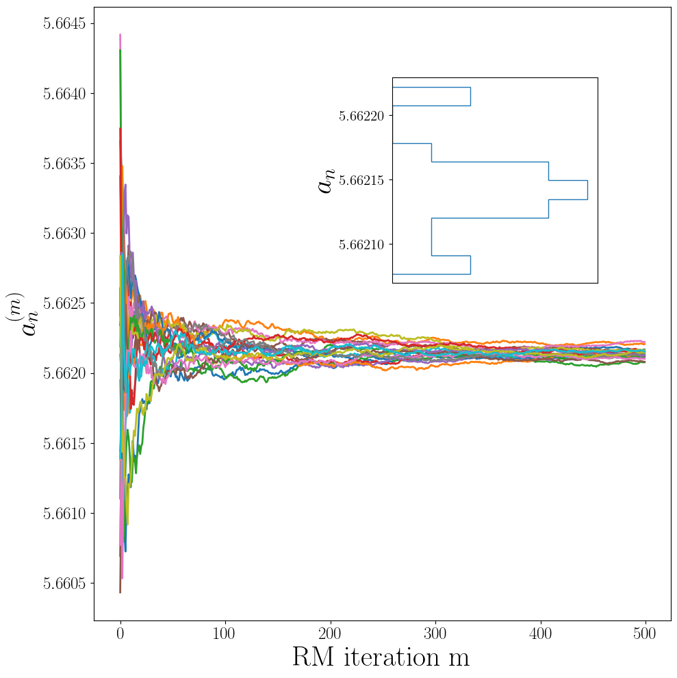
Figure 1: Twenty histories of $a_{n}^{(m)}$ as they are updated through 500 RM iterations, in different colours. This example is for a system with energy interval size $a^{4}\Delta_{E}/(6\tilde{V})=0.0007$, and the interval centered at $u_{p}=0.540676$. The inset shows the distribution of the final $a_{n}$ values.

In order to verify the convergence of the Robbins-Monro algorithm, we study the distribution of the value of $a_{n}^{(m)}$, for each energy interval, as a function of the iteration number, $m$. An example of this process is displayed in Fig. 1, for the energy interval centred at $a^{4}E_{n}/(6\tilde{V})=0.459324$ $(u_{p}=0.540676)$, with $a^{4}\Delta_{E}/(6\tilde{V})=0.0007$. The figure shows in different colours twenty independent Robbins-Monro trajectories. The trajectories are characterised by large oscillations at small $m$, followed by convergence to a common value at large $m$. The distribution of the asymptotic behaviour of the final values has standard deviation that scales as $\sim 1/\sqrt{m}$. On the basis of extensive test runs, we identified $\tilde{m}=500$ iterations of the RM algorithm as providing a good estimate of $a_{n}$. We verified that by this stage the twenty final estimates are normally distributed around their average value.

Table 3: The values of $\Delta_{E}$ used for this analysis, for each choice of the number of intervals, $2N-1$, in the energy range $\left[E_{\mathrm{\rm min}},\,E_{\mathrm{\rm max}}\right]$. The four-dimensional lattice has space-time volume $\tilde{V}/a^{4}=4\times 20^{3}$. Numerical values have been rounded to 4 decimal places for convenience.

$2N-1$	$\frac{a^{4}}{6\tilde{V}}\Delta_{E}$	$\frac{a^{4}}{6\tilde{V}}E_{\rm min}$	$\frac{a^{4}}{6\tilde{V}}E_{\rm max}$
$8$	$0.0063$	$0.4374$	$0.4659$
$15$	$0.0030$	$0.4380$	$0.4619$
$28$	$0.0015$	$0.4387$	$0.4604$
$55$	$0.0007$	$0.4391$	$0.4601$
$108$	$0.0004$	$0.4394$	$0.4598$

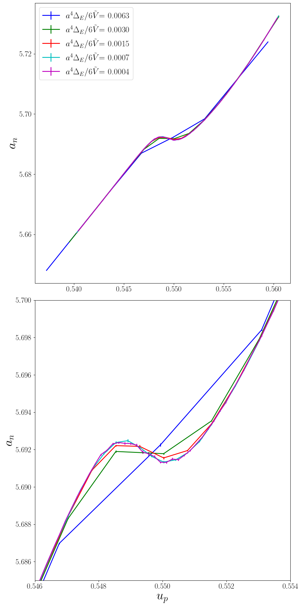
Figure 2: Measurements of $a_{n}$, plotted against $u_{p}$ at the centre of the energy intervals. Errors are estimated by bootstrapping over 20 repeats. Each value of $a_{n}$ is the final result of $500$ iterations of the Robins-Monro algorithm, for a lattices with $\tilde{V}/a^{4}=4\times 20^{3}$. The different curves/colors refer to different choices of $\Delta_{E}$—see Table 3—with the roughest results corresponding to the largest choices of $\Delta_{E}$. The bottom panel is a detail of the top one, focusing on the region in which $a_{n}(u_{p})$ is not invertible.

To extrapolate our results towards the $\Delta_{E}\to 0$ limit, we vary the number of sub-intervals $2N-1$, and repeat the process of computing the estimates of $a_{n}^{(m)}$. The corresponding values of $a^{4}\Delta_{E}/(6\tilde{V})$, and of the intervals analysed, are reported in Tab. 3.

In Fig. 2, we show our measurements of $a_{n}$, with their uncertainty, as a function of $u_{p}=1-a^{4}E_{n}/(6\tilde{V})$. The different curves show the results for several different values of $\Delta_{E}$. For $\Delta_{E}$ sufficiently small ($a^{4}\Delta_{E}/(6\tilde{V})\leq 0.0030$), a characteristic limiting shape starts to emerge in $a_{n}$ as a function of $u_{p}$, with the presence of one local minimum, one local maximum, and an inflection point between them. The resulting non invertibility of $a_{n}(u_{p})$ is closely related to the qualitative features of $P_{\beta}(u_{p})$, as discussed in Sect. IV, and to the presence of a first-order phase transition. Setting $\Delta_{E}$ to smaller values, the curve $a_{n}(u_{p})$ becomes smoother, which reduces the magnitude of the systematic error due to $\Delta_{E}$ itself.

The probability distribution of the average plaquette is obtained from Eq. (24). Estimates of $P_{\beta}(u_{p})$ are displayed in Fig. 3. The solid blue lines are our results, obtained using the LLR method. We compare them directly with the orange dashed lines obtained by using the standard importance sampling approach. Agreement between the two is evident, yet small discrepancies are visible in the neighbourhood of the maxima and of the local minimum of $P_{\beta}(u_{p})$. We show a number of examples displaying a single peak, but for $\beta=5.69187$ two peaks of similar height are present. As explained in Sect. IV, this is the expected signal of a first order phase transition.

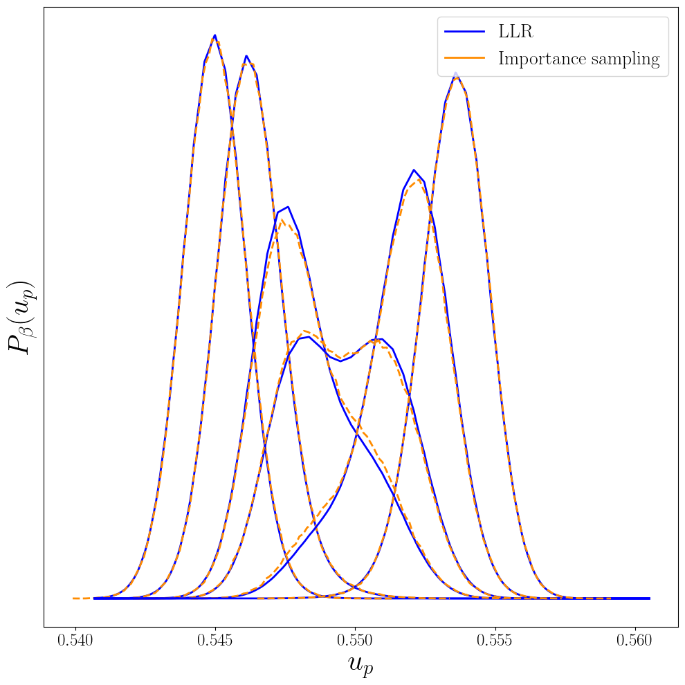
Figure 3: The probability distribution, $P_{\beta}(u_{p})$, computed with LLR method with $a^{4}\Delta_{E}/\tilde{V}=0.0007$ and $\tilde{V}/a^{4}=4\times 20^{3}$ (solid blue), compared to the same probability distribution computed with the standard lattice method based upon importance sampling (dashed orange). The probability density for different values of the coupling $\beta$ are shown, from left to right: $\beta=5.68000$, $\beta=5.68500$, $\beta=5.69000$, $\beta=5.69187$, $\beta=5.69500$ and $\beta=5.70000$.

As discussed in Sect. II, after each RM update, configuration swaps are considered, to ensure ergodicity of the algorithm. Figure 4 shows the evolution of the full set of $\{a_{n}\}_{n=1}^{2N-1}$ against the RM iteration, m. Following the track of the colours on the diagram shows how the configurations are swapped. The clustering of values around $a_{n}\sim 5.692$ is due to non invertibility of $a_{n}(u_{p})$ in the critical region. The diagram shows that, although in general terms there is an appreciable rate of exchange of configurations, it appears to be less probable to exchange configurations across the two different phases.

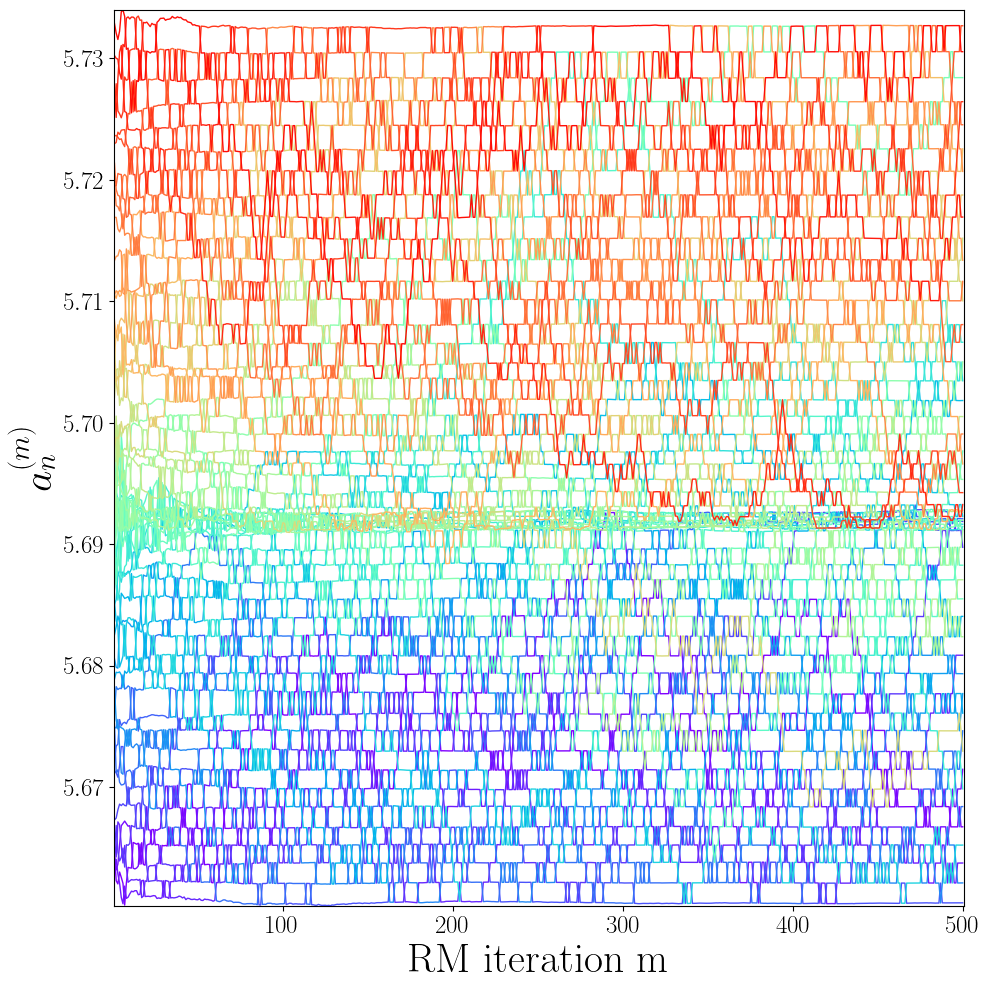
Figure 4: The trajectories of the set $\{a_{n}\}_{n=1}^{2N-1}$ are shown for 500 Robbins-Monro updates for a single run with configuration swaps included, for $a^{4}\Delta_{E}/(6\tilde{V})=0.0007$. The colours are determined by the energy interval that a given lattice system started in and follow them as they are exchanged between energy intervals.

V.1 Critical T and latent heat

The importance of the measurement of the critical value $\beta_{c}$ and of the position of the peaks of $P_{\beta_{c}}(u_{p})$ ($u_{p+}$ and $u_{p-}$) is explained in Sect. IV. In proximity of the transition at each value of $\beta$, a double gaussian function can be fitted to $P_{\beta}(u_{p})$, using the location of the local maxima and the width of the peaks as fitting parameters. The best-fit parameters are functions of $\beta$. An estimate of $\beta_{c}$ can then be obtained by solving the equation $|P_{+}-P_{-}|=0$, where $P_{+}=P_{\beta}(u_{p+})$ and $P_{-}=P_{\beta}(u_{p-})$, with the bisection method. The numerical values of $u_{p\,\pm}$ and $\beta_{c}$ can then used for the calculation of the latent heat through Eq. (26).

Figure 5: The double peak structure of the plaquette probability distribution, $P_{\beta}(u_{p})$, for $\beta=\beta_{c}=5.69196$ tuned to the critical point for this specific LLR run, when the two peaks have equal height. A double gaussian fitted at the peaks of the plots is shown in magenta (dashed), and compared with the blue (solid) line representing the LLR numerical results. We also show explicitly the location of the two peaks.

A representative example of the numerical results obtained from the LLR method, displaying also a fitted double gaussian, is displayed in Fig. 5. The agreement between the numerical and fitted curves is very good, with small deviations only appearing at the boundaries of the interval of $u_{p}$ depicted in the plot, which are not of primary importance in the fitting procedure.

Our estimates of $\beta_{c}$ and $\langle\Delta u_{p}\rangle_{\beta_{c}}$, for each choice of $\Delta_{E}$, are displayed in Figs. 6 and 7. The numerical values are reported in Tab. 4. We perform a linear fit of the behaviour of both $\beta_{c}$ and $\langle\Delta u_{p}\rangle_{\beta_{c}}$ as a function of $\Delta_{E}^{2}$. These fits are displayed in Figs. 6 and 7. We found the $\chi^{2}$ of the linear fit to be much less than 1. The origin of its smallness lies in the large error in the determination of $\beta_{c}$ at fixed $\Delta_{E}$. Several contributions to the errors of $\beta_{c}$ have been carefully analyzed and accounted for, except for those originating from the correlation between different subintervals (leading to correlations across each set of $a_{n}$) and the error on the fit of the double gaussian itself. Calculations in different subintervals would indeed be completely independent, were it not for the configuration swapping, which is necessary to achieve ergodicity in the sampling of configuration space. Since canonical observables, such as $P_{\beta}(u_{p})$, are determined from several values of $a_{n}$, they are affected by these autocorrelations. In order to approximately quantify the magnitude of these effects on the final estimate of $\beta_{c}$, we have computed this quantity from only half the $a_{n}$ estimates, i.e. only computed using the non-overlapping odd numbered energy intervals $\{a_{2n-1},E_{2n-1}\}_{n=1}^{N}$. The coarsest example in the plot ($a^{4}\Delta_{E}/\tilde{V}=0.0015$) has also been treated separately as it only contains a small number of intervals in the critical region. Extrapolations both including and excluding this point have been carried out, as well as an extrapolation using the points with only half the energy intervals. All extrapolations agree with one another within errors.

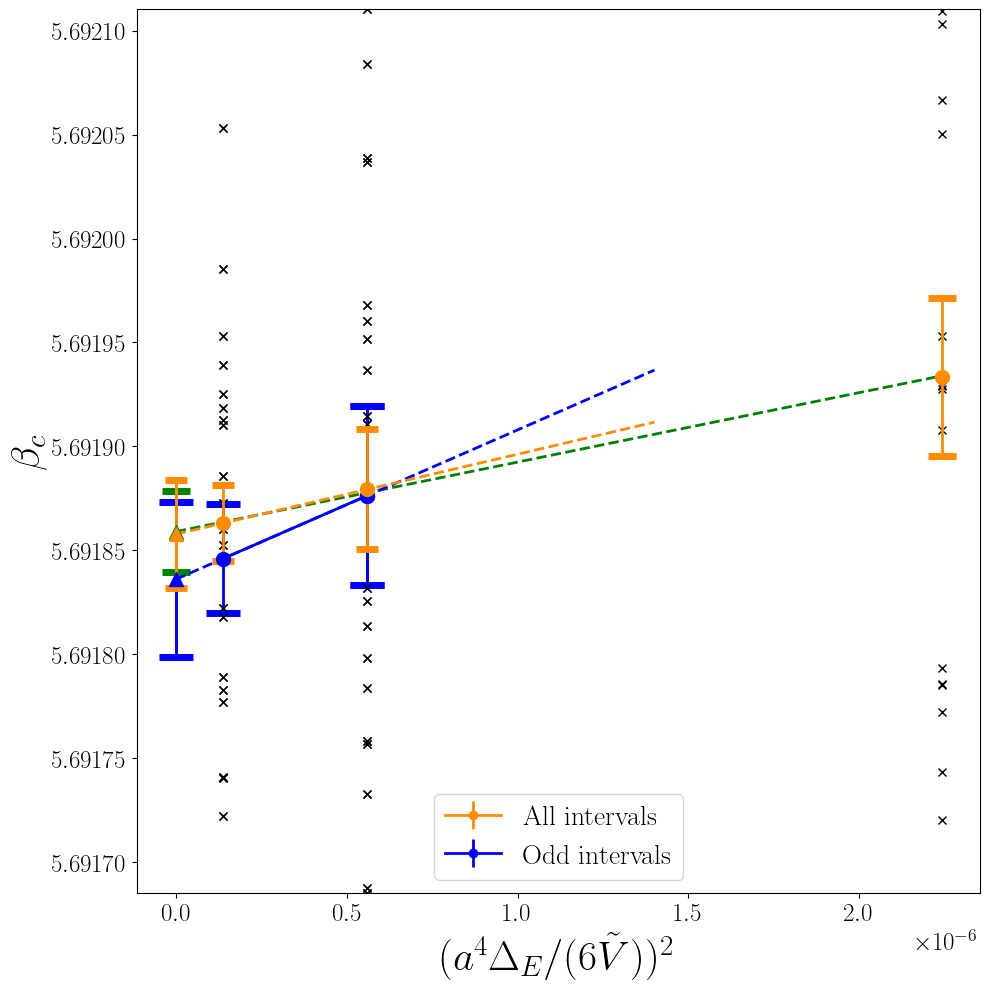
Figure 6: Estimates of the critical coupling $\beta_{c}$ as a function of the square of the energy interval, $\Delta_{E}^{2}$. The black crosses show the values of the critical coupling determined for each of the 20 repeats when all of the energy intervals are used in the determination of the plaquette distribution. The orange circles are the mean values of the black crosses and the error is found by bootstrapping them. The orange dashed line and triangle is a $\Delta_{E}\to 0$ extrapolation of the two finest results when all intervals are included, while the green dashed line shows the extrapolation of all three points. The blue circles show results when only the odd numbered intervals are used $\{a_{2n-1},E_{2n-1}\}_{n=1}^{N}$, an extrapolation to the $\Delta_{E}\to 0$ limit is shown by the blue line and the blue triangle. The coarsest point included in this graph only contains a small number of intervals in the critical region, making the double peak structure in the plaquette distribution difficult to resolve. All three final extrapolations are compatible with each other within errors.

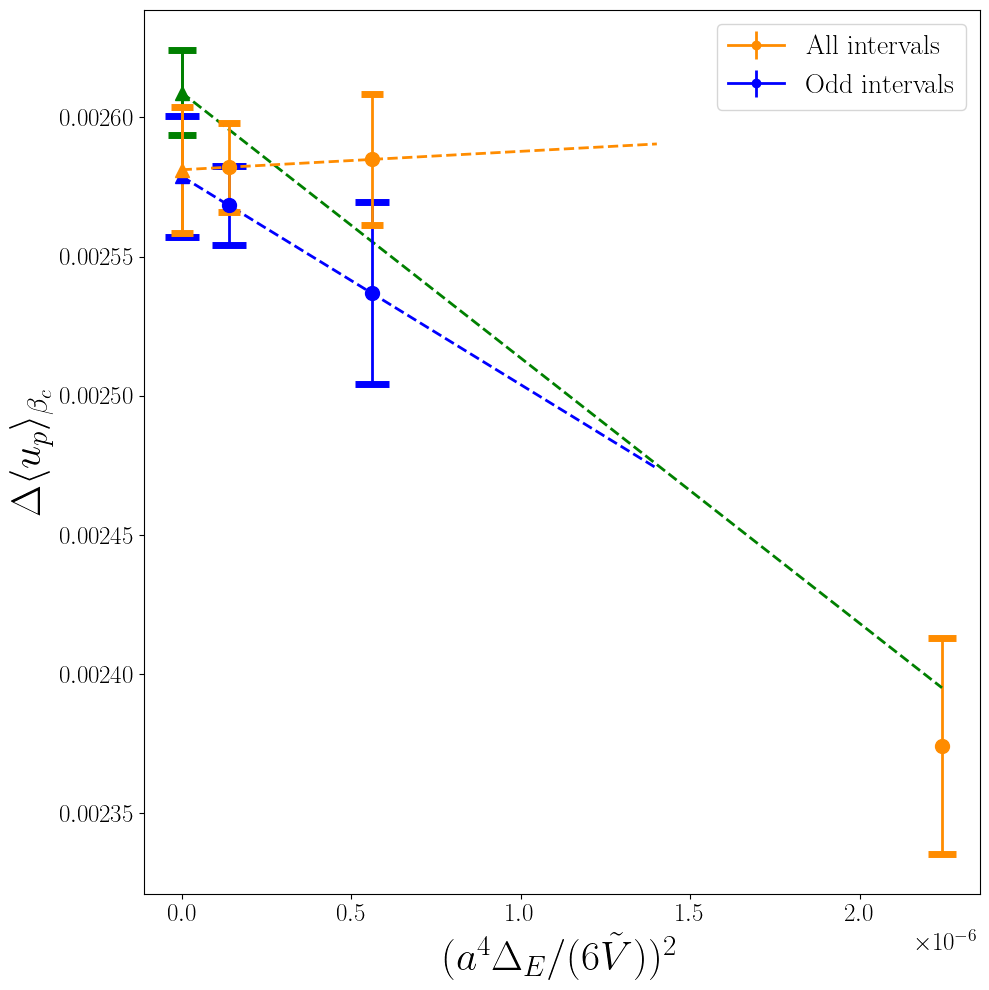
Figure 7: Estimates of the plaquette jump at the critical point, the difference between the plaquette values at the two peaks of the plaquette distribution when the double peak structure has peaks of equal height, as a function of the square of the energy interval, $\Delta_{E}^{2}$. The orange circles are the values found when all energy intervals are used to calculate the plaquette distribution, the error was found with a bootstrap procedure. The orange dashed line and triangle is an extrapolation of the two finest results when all intervals are included to the $\Delta_{E}\to 0$ limit, while the green dashed line shows the extrapolation of all three points. The blue circles show results when only the odd numbered intervals are used $\{a_{2n-1},E_{2n-1}\}_{n=1}^{N}$, an extrapolation to the $\Delta_{E}\to 0$ limit is shown by the blue line and the blue triangle. The coarsest point included in this graph only contains a small number of intervals in the critical region, making the double peak structure difficult to resolve. All three final extrapolations are compatible with each other within errors.

Table 4: The values of the critical coupling, $\beta_{c}$, and the difference between the peaks of the probability distribution at this coupling, $\Delta\langle u_{p}\rangle_{\beta_{c}}$, for different energy interval sizes $\Delta_{E}$. The table shows results obtained in two ways. Either all intervals are included or only the odd intervals, $\{a_{2n-1},E_{2n-1}\}_{n=1}^{N}$. The symbol ‘$\to 0$’ is used to denote the result of an extrapolation. The table contains three extrapolations. An extrapolation using the results when only odd intervals are considered, an extrapolation when all points with all the intervals are used and an extrapolation of the two finest interval sizes when all intervals are used. See also Ref.[86]

	$\frac{a^{4}\Delta_{E}}{6\tilde{V}}$	$\beta_{c}$	$\Delta\langle u_{p}\rangle_{\beta_{c}}$
Odd intervals	$0.0007$	$5.69188(4)$	$0.00254(3)$
Odd intervals	$0.0004$	$5.69185(3)$	$0.00257(2)$
All intervals	$0.0015$	$5.69193(4)$	$0.00237(4)$
All intervals	$0.0007$	$5.69188(3)$	$0.00258(2)$
All intervals	$0.0004$	$5.69186(2)$	$0.00258(2)$
Odd intervals	$\to 0$	$5.69184(4)$	$0.00258(2)$
All intervals all points	$\to 0$	$5.69186(3)$	$0.00258(2)$
All intervals 2 points	$\to 0$	$5.69186(2)$	$0.00261(2)$

V.2 Thermodynamic potentials

As discussed in Sect. IV, the LLR algorithm, through the estimation of $\rho(E)$, allows us to estimate the thermodynamic potentials of the bulk system. We focus our attention on the free energy, $F$, defined in Eq. (28), the entropy, $s$, defined in Eq. (29), and the (microcanonical) temperature, $t$, in Eq. (30). As we showed explicitly in Fig. 2, $a_{n}(u_{p})$ and therefore $t(E)$ is not globally invertible. Yet, we can study how $F$ evolves as a function of $t$, by piece-wise inverting $t(E)\leftrightarrow E(t)$.

In order to best expose the behaviour of $F(t)$, we consider a subtracted free energy, defined as $f=a^{4}(F(t)+\Sigma t)/(\tilde{V})$. The constant $\Sigma$, as we anticipated after Eq. (30), reflects the existence of an arbitrary additive constant in $s$, which we are now removing, with an approximate numerical procedure. The subtracted free energy is displayed in Fig. 8, as a function of (discretised) $t=1/a_{n}$. For the purpose of producing this figure, $\Sigma$ has been calculated as the average of the entropy over the interval of (microcanonical) temperatures displayed in the plot—which would correspond to the average gradient of the curve. This rough estimate is not equivalent to imposing the third law of thermodynamics ($\lim_{t\rightarrow 0}s=0$), but suffices for our current purposes, and allows us to avoid the expensive process of repeating the LLR procedure for choices of $E_{n}$ that lie far away from the critical region.

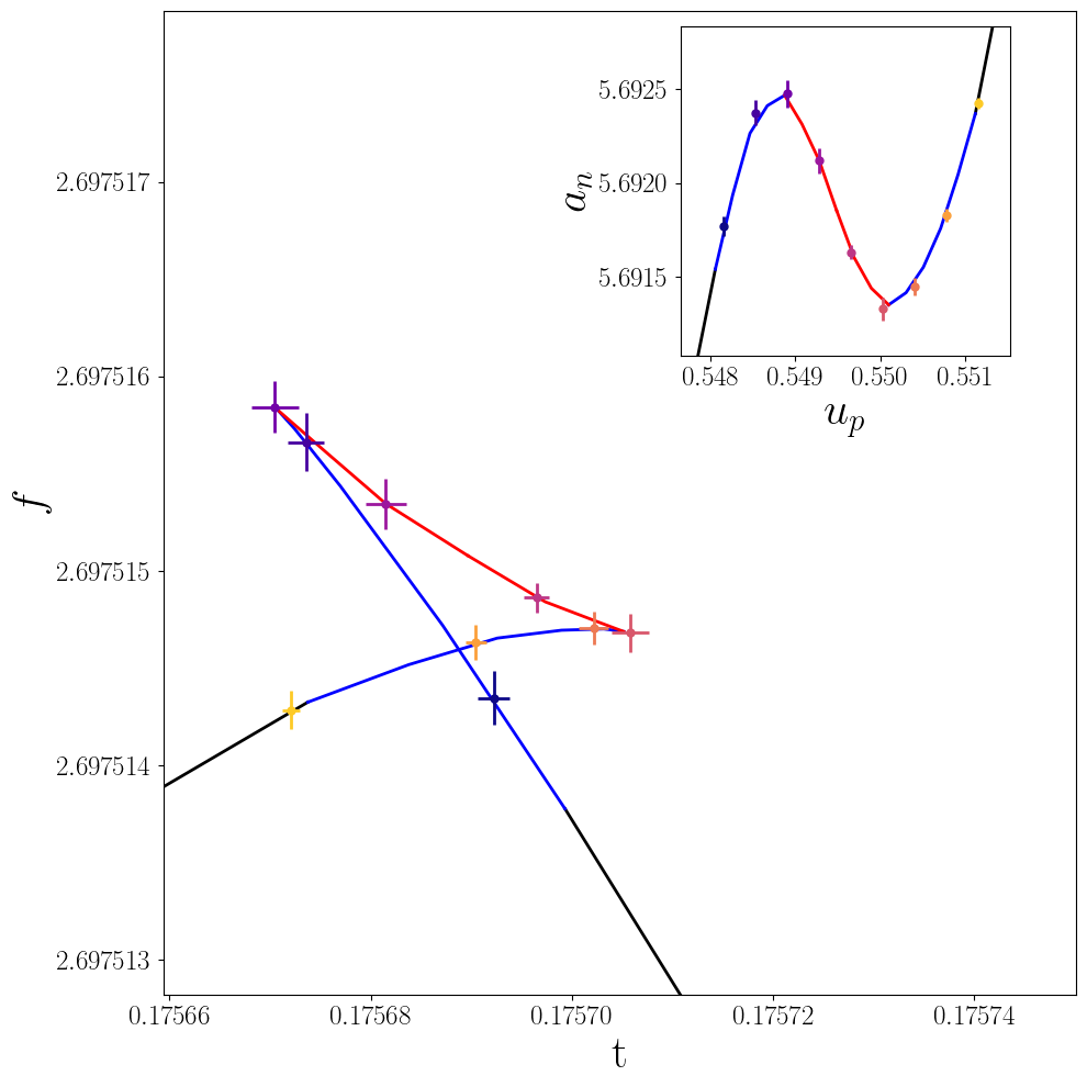
Figure 8: The (subtracted) free energy, $f$, as a function of the (discretised, microcanonical) temperature $t=1/a_{n}$. $f$ is defined in the main body of the text. The dots (with errors) represent the values of $f$ corresponding to the centre of each energy interval used in the LLR algorithm, while the solid line is reconstructed by piece-wise linearly interpolation of $a_{n}(u_{p})$. The color coding of the points and solid lines are chosen to match those in the inset, displaying our numerical results for $a_{n}(u_{p})$. In black we show the regions of $t$ for which $f$ is single-valued, in blue we show the (meta-)stable solutions within the region where $f$ is multi-valued, and in red the unstable (tachyonic) branch of solutions. The dots follow a colormap in the value average plaquette, with darker colors corresponding to smaller $u_{p}$.

In Fig. 8, the uncertainty in the numerical extraction of $a_{n}$ affects both axes of the plot. The values of $f$ corresponding to the piece-wise linear interpolation are represented in the main plot as colored lines. The plot clearly shows the multi-valued nature of the free energy, the location of the temperature corresponding to criticality in the thermodynamic limit, and details about stable, metastable and tachyonic branches of configurations of the system. The discontinuity in the first derivative is located at $t_{c}\simeq 0.175690$, which is the temperature at which the system undergoes a first-order phase transition.

The relation between different branches of $F(t)$ and physical stability is illustrated in Fig. 9. The inverse temperature $a_{n}$ is displayed as a function of $u_{p}=1-a^{4}E_{n}/6\tilde{V}$ in the top panel. The plaquette probability distribution at the critical point, $P_{\beta_{c}}(u_{p})$, is depicted in the middle panel. The corresponding effective potential is plotted in the bottom panel. While the two configurations corresponding to maxima of $P_{\beta_{c}}(u_{p})$ are both absolute minima of the effective potential, a third configuration, corresponding to a local minimum of the probability, is a local maximum of the effective potential.

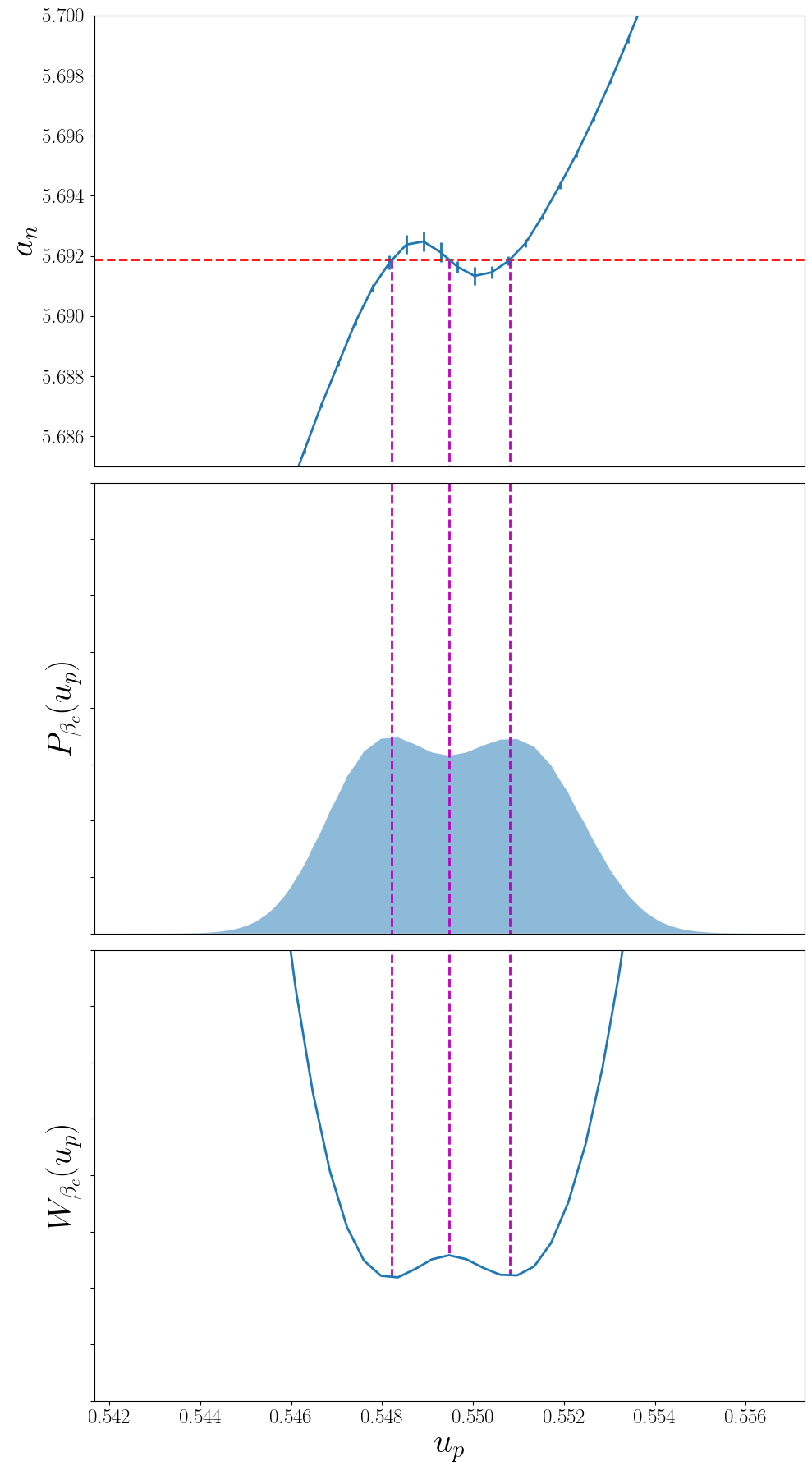
Figure 9: Top panel: $a_{n}$ ($=1/t_{n}$) against $u_{p}$ at the centre of the energy intervals, in close proximity of the critical region. Middle panel: the reconstructed plaquette distribution, $P_{\beta}(u_{p})$, at critical coupling $\beta_{c}=5.69187$. Bottom panel: quantum effective potential for the plaquette at the critical coupling. The red line in the top plot shows the critical value of the coupling and its relation to the microcanonical temperature, $a_{n}$. The magenta (vertical, dashed) lines show the locations at which the red line intersects the curve $a_{n}(u_{p})$.

VI Outlook

With this paper, we set the basis of a systematic research programme that exploits the properties of the LLR method to yield future high precision measurements characterising lattice gauge theories in proximity of the confinement/deconfinement phase transition. The method is powerful and promises to yield information that is difficult to access otherwise, as it modifies Monte Carlo sampling by restricting it to arbitrarily small energy windows. It hence provides numerical access to the details of the physics in regions of parameter space exhibiting all the typical feature of first-order phase transitions: phase coexistence, metastability and/or instability of multiple branches of solutions, non-invertibility and/or multi-valuedness of some state function.

We showed how the information from these energy-bound Monte Carlo feeds into recursive relations (e.g., an implementation of the Robbins-Monro algorithm) that can determine the density of states for any interesting range of energies. And we provided explicit relations between the density of states and observables such as the critical temperature and the latent heat. Furthermore, we found that the results for the density of states can be recast in terms of an effective free energy and an effective potential that exhibit with spectacular level of resolution the details of the physics near the transition.

We restricted this study to the $SU(3)$ lattice Yang-Mills theory, and performed it with one choice of lattice parameters, fixing $N_{L}=20$ and $N_{T}=4$. The trademark of the LLR algorithm is that we found clear evidence of the first-order nature of the transition, without the need of a finite-volume study, and an extrapolation of the scaling to large volumes. The physically interesting observables need to be extrapolated to the continuum and infinite-volume limits, with dedicated, extensive numerical work, which would allow for a direct comparison with results that use different numerical techniques. In the future we plan to repeat the process with larger values of both $N_{T}$ and $N_{L}$, which will provide us with control over lattice systematics.

We plan to apply this process to other theories, in particular those based on the sequence of symplectic groups $Sp(2N)$, which might play an important role in models of dark matter, and hence in the physics of the early universe, by yielding a potentially detectable stochastic background of gravitation waves. In particular, the precise measurement of the effective potential, $W_{\beta}(u_{P})$, the results of which are exemplified in Fig. 9, can be used to obtain a precise determination not just of the parameter, $\alpha$, controlling the strength of the phase transition, but also of the inverse duration of the transition, $\beta/H_{\ast}$. The latter is challenging to estimate from first principle, yet it is necessary in the calculation of the power-spectrum of stochastic gravitational waves, $h^{2}\Omega_{GW}$.

There are still some limitations to what we are able to do at this stage of development of this technique, and we would like to address them in the future. The first such challenge has to do with scalability and parallelisation of the algorithm and software: the attentive reader will certainly be aware of the fact the energy constraint we are imposing is globally defined on the whole lattice configuration, a constraint that cannot be immediately parallelised, because it requires communication between different parallel subprocesses. This obstruction can be circumvented by partitioning the system in domains, and allowing for the information about the total energy to be shared across processes living in separate domains. But optimisation of this process is a non-trivial open problem. Related to scalability is also the fact that when we tested the algorithm on larger volumes, we found a weakening of the transition, which makes it more difficult to detect. Whether this is an intrinsic feature of the algorithm, or a consequence of the choice of theory—$SU(3)$ is believed to undergo a weak first-order phase transition—is an open problem.

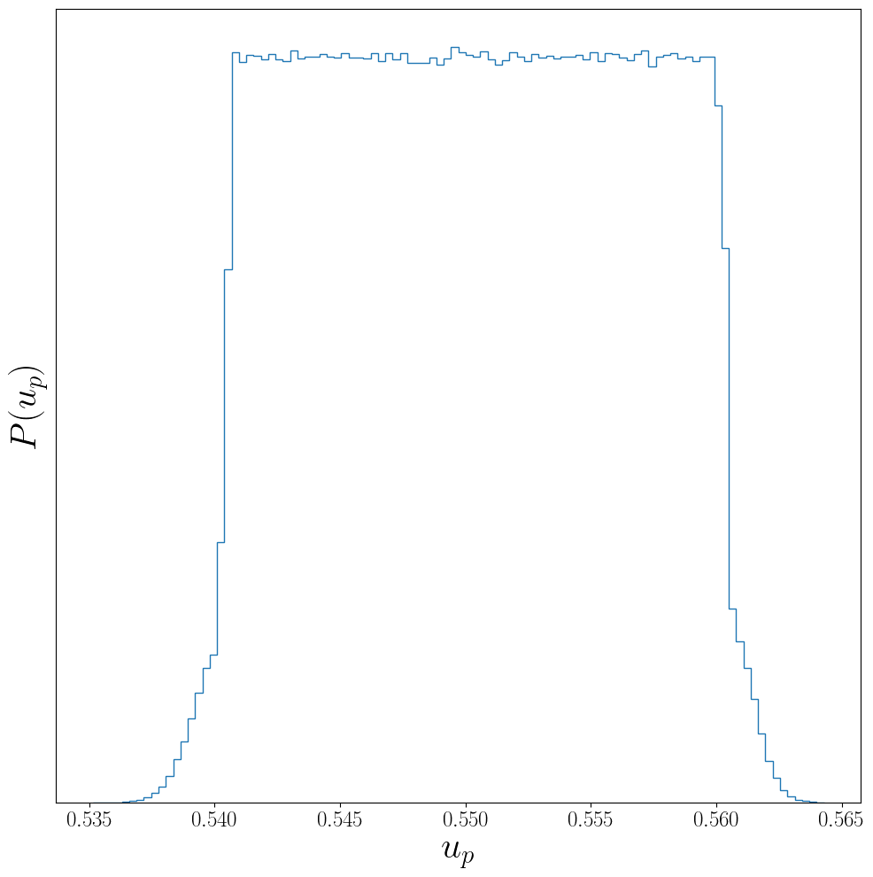
Figure 10: For one LLR run with $a^{4}\Delta_{E}/6\tilde{V}=0.0007$, the distribution of measured average plaquette values for all intervals is plotted for configurations restricted to a given energy interval, updated with a fixed value of $a_{n}$. Within the plaquette range, $a^{4}E_{\mathrm{min}}/6\tilde{V}\leq 1-u_{p}\leq a^{4}E_{\mathrm{max}}/6\tilde{V}$, the distribution is approximately flat, while the boundary intervals have gaussian tails allowing configurations to escape the energy boundaries, resolving the residual ergodicity problems.

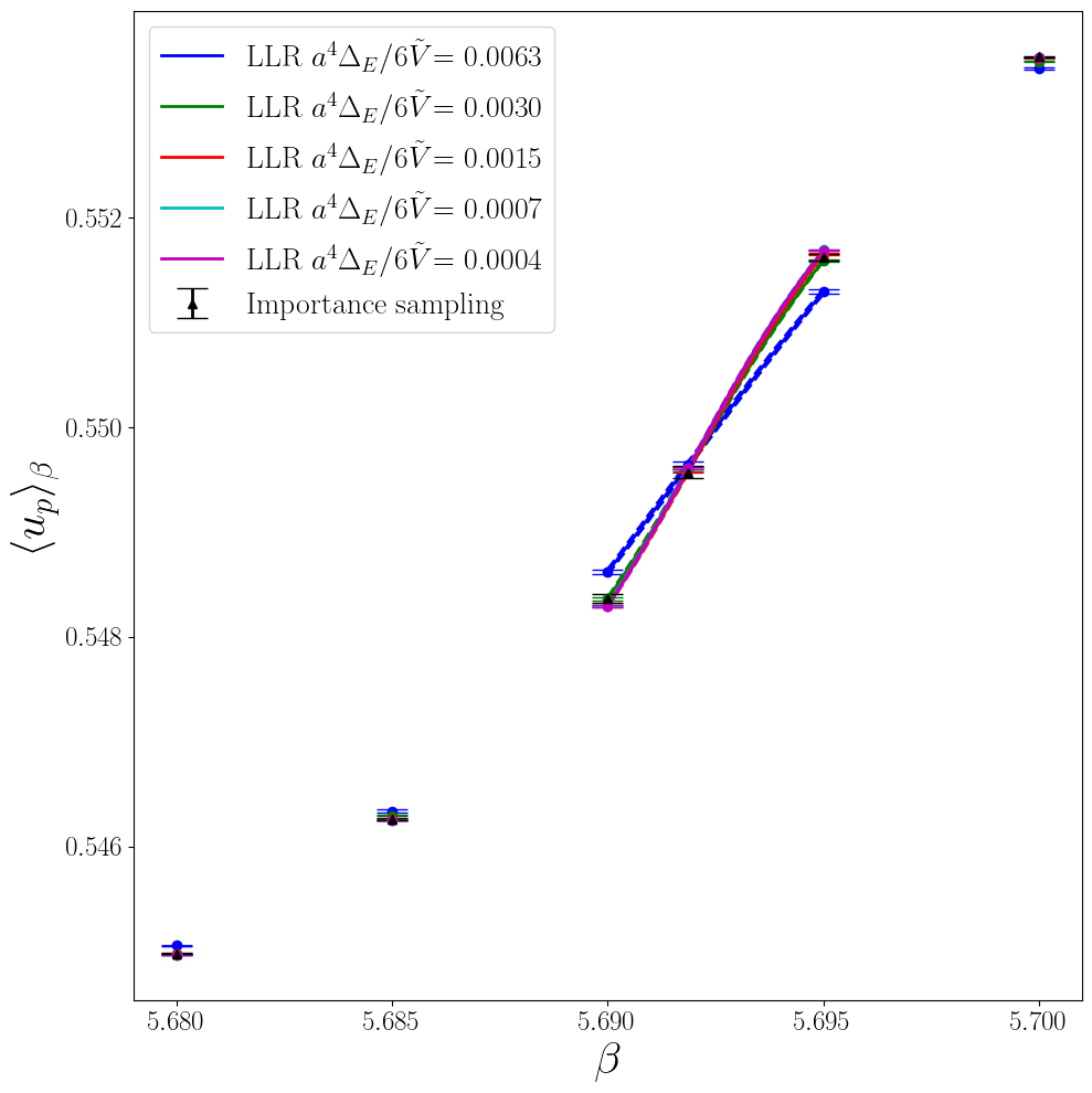
Figure 11: The vacuum expectation value of the average plaquette for different couplings calculated using the LLR method for different $a^{4}\Delta_{E}/(6\tilde{V})$ sizes, and compared to the measurement from importance sampling methods (black triangles). In both cases the lattice size is $\tilde{V}/a^{4}=4\times 20^{3}$. The dots are at a coupling with a direct comparison to the importance sampling. The solid lines are a finer scan around the critical region, containing 1000 points evenly spaced between 5.690 and 5.695. The errors on this line are calculated by bootstrapping over the repeats and are represented by the dashed curves.

Finally, a more conceptual set of questions arises in view of applications: we showed that we can compute an effective potential, without the need to build an intermediate effective field theory treatment based on simplifying assumptions for the functional dependence on the order parameter. It would be useful to understand how this feature can be exploited for phenomenological purposes. For example, is the detailed knowledge of the effective potential going to improve current understanding of the amplitude of gravitational waves arising in the early universe?

All these and other interesting questions are left for what we foresee to become an interesting and original research programme, which we are planning to develop in the near and long-term future.

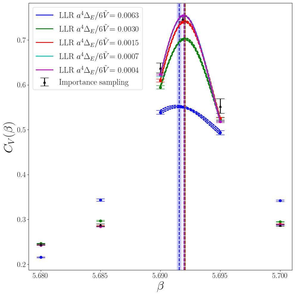
Figure 12: The specific heat for different couplings calculated using the LLR method for different values of $a^{4}\Delta_{E}/(6\tilde{V})$ sizes, and compared to the measurement from importance sampling methods (black triangles). In both cases the lattice size is $\tilde{V}/a^{4}=4\times 20^{3}$. The dots are at a coupling with a direct comparison to the importance sampling. The solid lines are a finer scan around the critical region, containing 1000 points evenly spaced between 5.690 and 5.695. The errors on this line are calculated by bootstrapping over the repeats and are represented by the dashed curves. The extrema of the curve for all $a^{4}\Delta_{E}/(6\tilde{V})$ sizes are shown by the vertical dashed lines, with the corresponding error represented by the shaded region. The extrema of all but the coarsest interval sizes overlap.

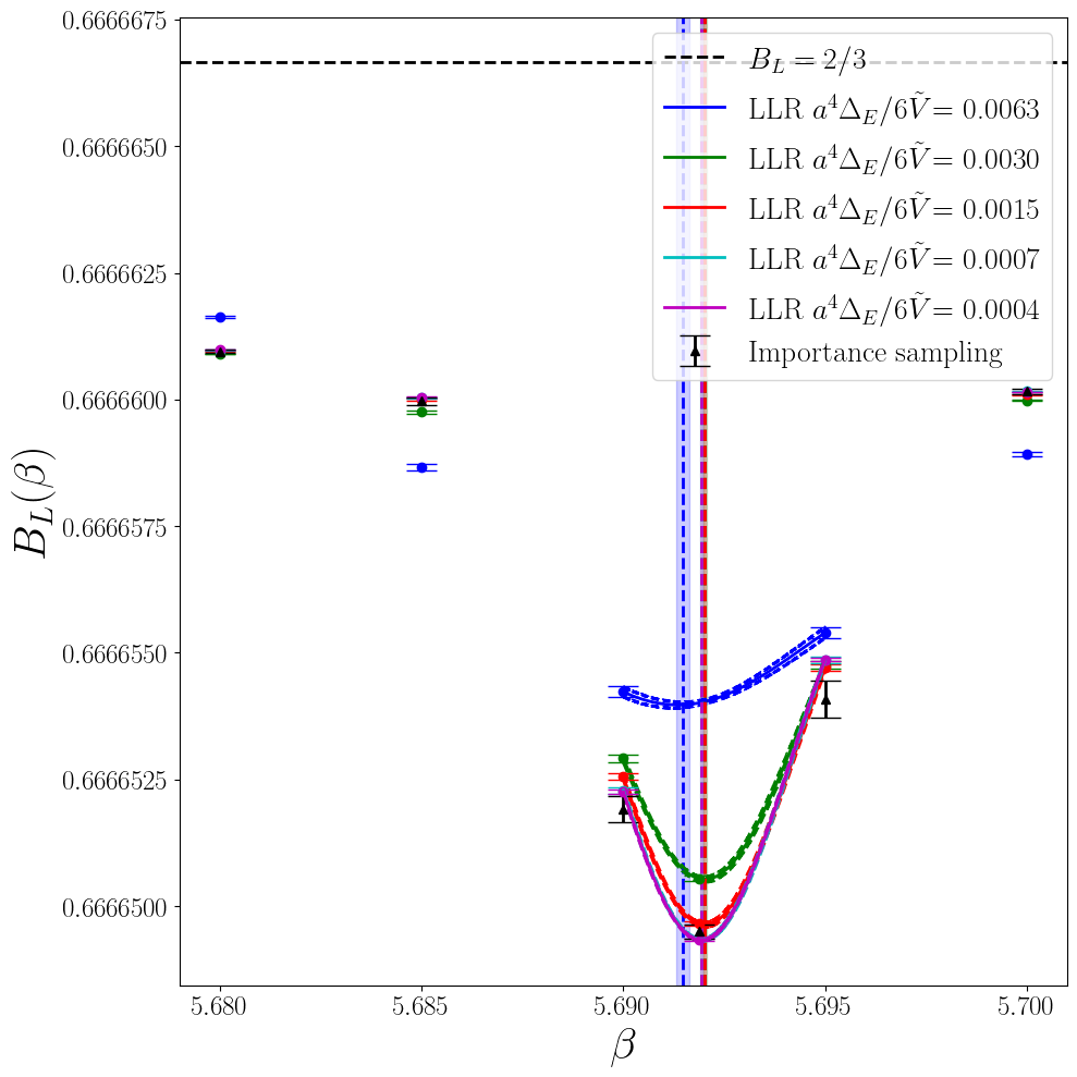
Figure 13: The Binder cumulant for different couplings calculated using the LLR method for different values of $a^{4}\Delta_{E}/(6\tilde{V})$ sizes, and compared to the measurement from importance sampling methods (black triangles). In both cases the lattice size is $\tilde{V}/a^{4}=4\times 20^{3}$. The dots are at a coupling with a direct comparison to the importance sampling. The solid lines are a finer scan around the critical region, containing 1000 points evenly spaced between 5.690 and 5.695. The errors on this line are calculated by bootstrapping over the repeats and are represented by the dashed curves. The extrema of the curve for all $a^{4}\Delta_{E}/(6\tilde{V})$ sizes are shown by the vertical dashed lines, with the corresponding error represented by the shaded region. The extrema of all but the coarsest interval sizes overlap.

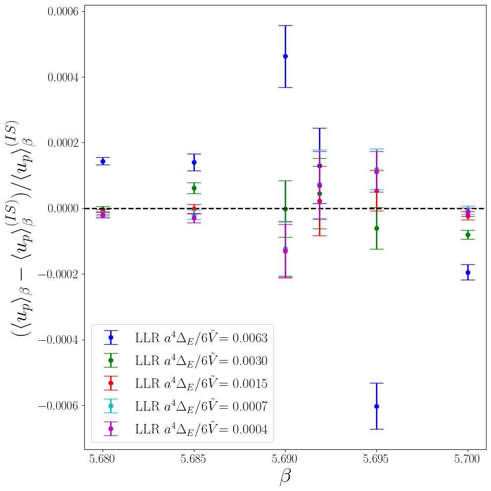
Figure 14: The relative change for the vacuum expectation value of the average plaquette calculated between the LLR method and importance sampling (IS) method results is shown at different couplings. In both cases the lattice size is $\tilde{V}/a^{4}=4\times 20^{3}$. The coloured dots show the results for different values of $a^{4}\Delta_{E}/(6\tilde{V})$. The errors were found by using bootstrap methods to calculate the error on LLR and importance sampling results separately, then propagating them.

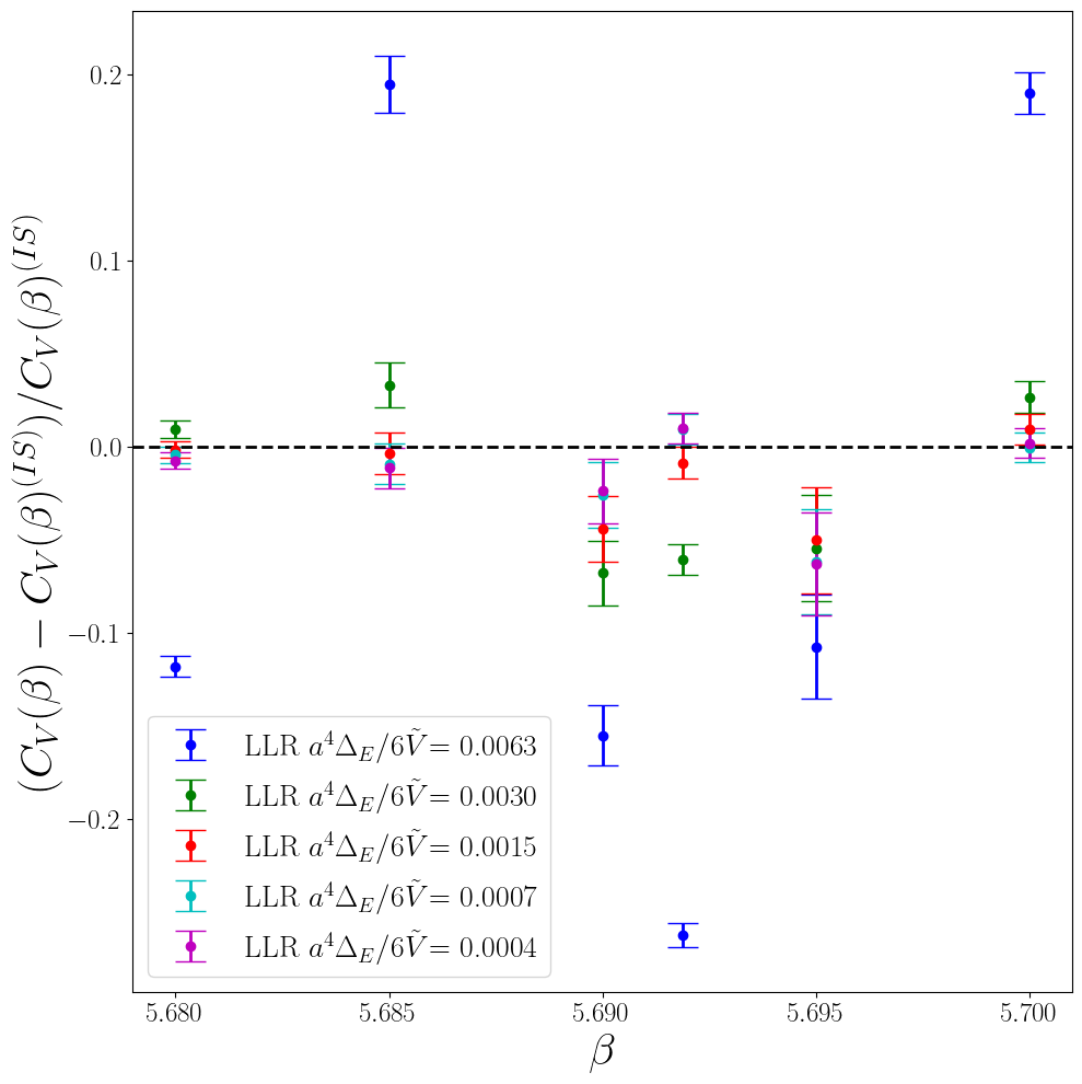
Figure 15: The relative change for the specific heat calculated between the LLR method and importance sampling (IS) method results is shown at different couplings. In both cases the lattice size is $\tilde{V}/a^{4}=4\times 20^{3}$. The coloured dots show the results for different values of $a^{4}\Delta_{E}/(6\tilde{V})$. The errors were found by using bootstrap methods on the LLR and importance sampling results separately, then propagating them.

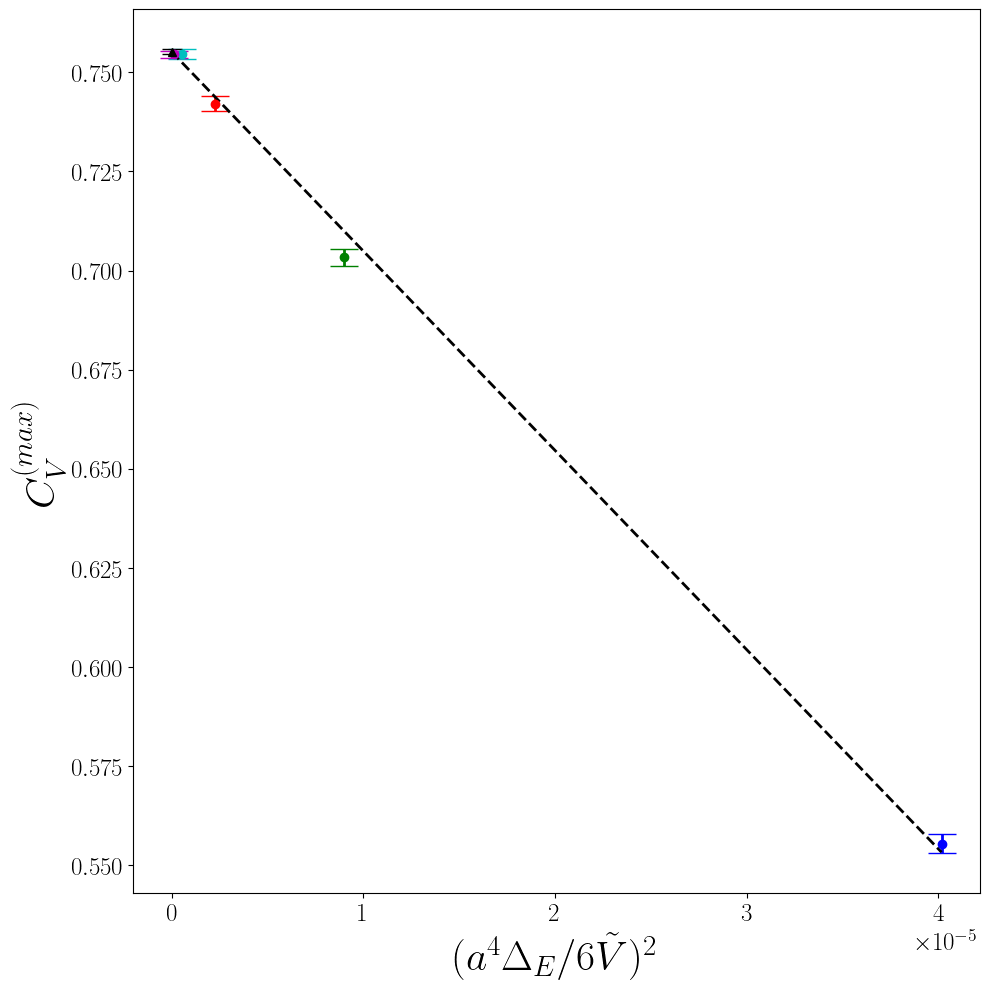
Figure 16: The maximum value of the specific heat calculated using the LLR method for couplings around the critical region, containing 1000 points evenly spaced between 5.690 and 5.695, is plotted against the $(a^{4}\Delta_{E}/(6\tilde{V}))^{2}$ value it was calculated at. The errors on each point are found by bootstrapping the repeats. The black dot shows the limit of $(a^{4}\Delta_{E}/(6\tilde{V}))^{2}\to 0$ and its errors, found by a linear fit. The lattice size is $\tilde{V}/a^{4}=4\times 20^{3}$.

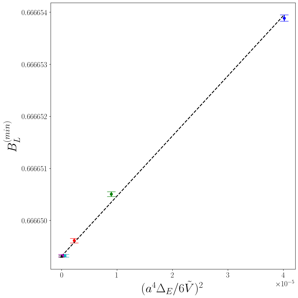
Figure 17: The minimum value of the Binder cumulant calculated using the LLR method for couplings around the critical region, containing 1000 points evenly spaced between 5.690 and 5.695, is plotted against the $(a^{4}\Delta_{E}/(6\tilde{V}))^{2}$ value it was calculated at. The errors on each point are found by bootstrapping the repeats. The black dot shows the limit of $(a^{4}\Delta_{E}/(6\tilde{V}))^{2}\to 0$ and its errors, found by a linear fit. The lattice size is $\tilde{V}/a^{4}=4\times 20^{3}$.

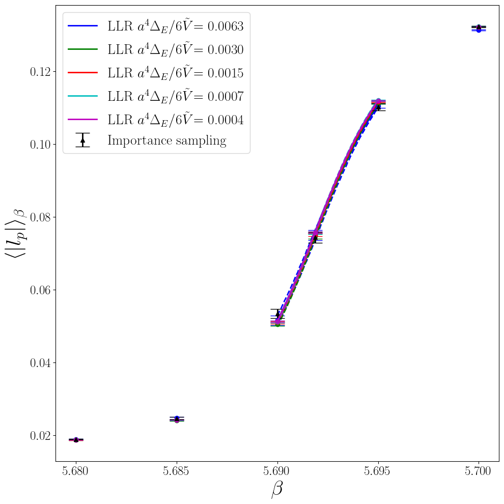
Figure 18: The vacuum expectation value of the absolute value of the Polyakov loop for different couplings calculated using the LLR method for different values of $a^{4}\Delta_{E}/(6\tilde{V})$, and compared to the measurement from importance sampling methods (black triangles). In both cases the lattice size is $\tilde{V}/a^{4}=4\times 20^{3}$. The dots are at a coupling with a direct comparison to the importance sampling. The solid lines are a finer scan around the critical region, containing 100 points evenly spaced between 5.690 and 5.695. The errors on this line are calculated by bootstrapping over the repeats and are represented by the dashed curves. For the values determined with the LLR method, the calculation requires measurements of the Polyakov loop on a set of configurations found using the restricted energy updates, with $a_{n}$ fixed to its final value. For these calculations 40000 fixed $a_{n}$ measurements were performed on all the intervals.

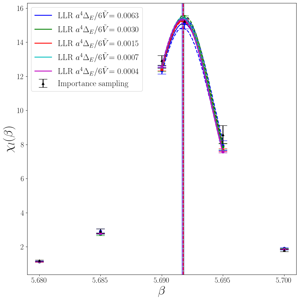
Figure 19: The Polyakov loop susceptibility for different couplings calculated using the LLR method for different values of $a^{4}\Delta_{E}/(6\tilde{V})$, and compared to the measurement from importance sampling methods (black triangles). In both cases the lattice size is $\tilde{V}/a^{4}=4\times 20^{3}$. The dots are at a coupling with a direct comparison to the importance sampling. The solid lines are a finer scan around the critical region, containing 100 points evenly spaced between 5.690 and 5.695. The errors on this line are calculated by bootstrapping over the repeats and are represented by the dashed curves. For the values determined with the LLR method, the calculation requires measurements of the Polyakov loop on a set of configurations found using the restricted energy updates, with $a_{n}$ fixed to its final value. For these calculations 40000 fixed $a_{n}$ measurements were performed on all the intervals. The extrema of the curve for all $a^{4}\Delta_{E}/(6\tilde{V})$ sizes are shown by the vertical dashed lines, with the corresponding error represented by the shaded region. The extrema of all interval sizes overlap.

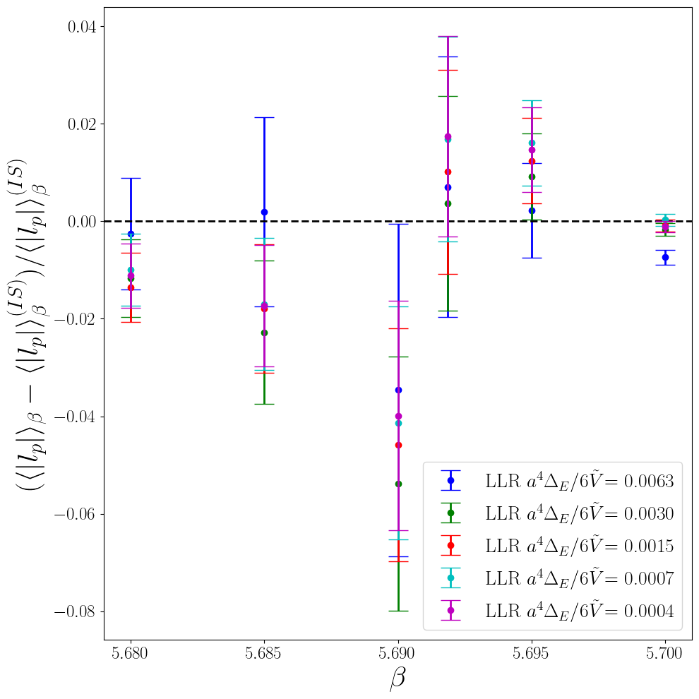
Figure 20: The relative change in the vacuum expectation value of the absolute value of the Polyakov loop, calculated between the LLR method and the importance sampling (IS) method results, is shown at different couplings. In both cases the lattice size is $\tilde{V}/a^{4}=4\times 20^{3}$. The coloured dots show the results for different values of $a^{4}\Delta_{E}/(6\tilde{V})$. The error is found by using bootstrap methods on LLR and importance sampling results separately, then propagating them. For the values determined with the LLR method, the calculation requires measurements of the Polyakov loop on a set of configurations found using the restricted energy updates, with $a_{n}$ fixed to its final value. For these calculations 40000 fixed $a_{n}$ measurements were performed on all the intervals.

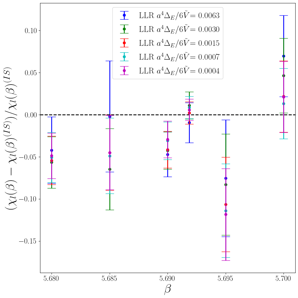
Figure 21: The relative change in the Polyakov loop susceptibility, calculated between the LLR method and importance sampling (IS) method results, is shown at different couplings. In both cases the lattice size is $\tilde{V}/a^{4}=4\times 20^{3}$. The coloured dots show the results for different values of $a^{4}\Delta_{E}/(6\tilde{V})$. The error is found by using bootstrap methods on LLR and importance sampling results separately, then propagating them. For the values determined with the LLR method, the calculation requires measurements of the Polyakov loop on a set of configurations found using the restricted energy updates, with $a_{n}$ fixed to its final value. For these calculations 40000 fixed $a_{n}$ measurements were performed on all the intervals.

Appendix A Constraint-preserving update proposals

In this appendix, we present our strategy for sampling random configurations from the probability density

$$dP_{c}(U)\propto dP(U)\theta(E-E_{n-1})\theta(E_{n+1}-E)\,,$$ (31)

where $dP(U)$ is the unconstrained probability density associated to the link variable $U$, and the $\theta$ functions that implement the energy constraints, $E_{n-1}=E_{n}-\Delta_{E}/2\leq E\leq E_{n}+\Delta_{E}/2=E_{n+1}$.

The problem of sampling $dP(U)$ has been elegantly solved in Ref. [170] for the gauge group $SU(2)$, and then generalised to $SU(N_{c})$ gauge groups in Ref. [171]. In the case $N_{c}=2$,

$$dP(U)\propto dU\exp\left\{-\frac{\beta}{2}{\rm Re}\left[{\rm Tr}\left(U\frac{}{}U_{\sqcup}\right)\right]\right\}\,,$$ (32)

where $U_{\sqcup}$ is the staple around $U$, and $dU$ is the Haar measure of the gauge group. Any $SU(2)$ matrix $U_{p}/k=UU_{\sqcup}/k$ can be parameterised as $U_{p}/k=u_{0}\mathbb{I}_{2}+i\,\vec{u}\cdot\vec{\tau}$, where $\vec{\tau}$ are the Pauli matrices, $u_{\mu}$ are real numbers satisfying the normalisation $\sum_{\mu}u_{\mu}^{2}=1$ and $k\equiv{\rm det}(U_{\sqcup})$. The matrix $U_{p}/k$ is obtained by first sampling $\vec{u}$ uniformly on a sphere of radius $\sqrt{1-u_{0}^{2}}$, and then $u_{0}$ from the probability distribution

$$d\tilde{P}(u_{0})\sim du_{0}\sqrt{1-u_{0}^{2}}\exp\left\{\beta\,k\frac{}{}u_{0}\right\}~{}.$$ (33)

We determine $u_{0}$ as

$$u_{0}=\frac{1}{\beta k}\log{\left(e^{-\beta k}+\xi(e^{\beta k}-e^{-\beta k})\right)},$$ (34)

where $0\leq\xi\leq 1$ is a uniform random variable, and then perform an accept-reject step to correct for the presence of the factor $\sqrt{1-u_{0}^{2}}$ in Eq. (33).

We further generalise these ideas to take into account, in the Monte Carlo evolution, the presence of the constraints $E_{n-1}\leq E\leq E_{n+1}$. Consider the variation in the total energy $E$ due to the update of a specific link variable. Let $E_{i}$ ($E_{f}$) be this energy contribution before (after) the update. The energy constraints after the update are

$$E_{n-1} \leq E-E_{i}+E_{f}\,\leq\,E_{n+1}\,.$$ (35)

Since $E_{f}=2(d-1)-ku_{0}$, where $d$ is the number of space-time dimensions, the above constraint can be expressed as $u_{\rm min}<u_{0}<u_{\rm max}$ where

$$u_{\mathrm{min}} =\max{\left(\frac{2(d-1)+(E-E_{n+1})-E_{i}}{k},-1\right)}~{},$$ (36)

$$u_{\mathrm{max}} =\min{\left(\frac{2(d-1)+(E-E_{n-1})-E_{i}}{k},1\right)}~{}.$$ (37)

These constraints can be enforced on the random sampling of $u_{0}$ by setting

$$u_{0}=\frac{1}{\beta k}\log\left(e^{\beta ku_{\rm min}}+\xi(e^{\beta ku_{\rm max}}-e^{\beta ku_{\rm min}})\right),$$ (38)

where, as in Eq. (34), $0\leq\xi\leq 1$ is sampled uniformly, and an accept-reject step is performed to correct for the presence of the factor $\sqrt{1-u_{0}^{2}}$.

The constrained heat-bath algorithm outlined above can be generalised to $SU(N_{c})$ gauge groups following the Cabibbo-Marinari process suggested in Ref. [171]. The contribution of each $SU(2)$ subgroup of a $SU(N_{c})$ link variable to the total energy of the system is additive. Thus, the constraint can be solved independently for each $SU(2)$ subgroup of each link variable. It is easy to show that the constrained probability density of $U$ is invariant under $U\rightarrow\alpha_{k}U$, where $\alpha_{k}$ is an element of one of the $SU(2)$ subgroups of $SU(N_{c})$.

Appendix B Further technical details on the algorithm and parallelism

To improve the scalability of the LLR algorithm when moving to larger lattice sizes, domain decomposition was implemented, in which the full lattice is split into subdomains, which can be processed separately. The restricted heat-bath updates, discussed in Appendix A, require prior knowledge of the total action of the system and will change it’s value. Therefore, the restricted heat-bath update cannot occur in multiple subdomains simultaneously.

To circumvent this issue, in this work, domain decomposition is instead built out of a combination of restricted local heat-bath updates and the inherently micro-canonical over-relaxation updates. This ensures the value of the total action is only changed in one subdomain at a time. If we have a lattice with $N_{D}$ subdomains, during each sweep, one domain is updated with a local heat-bath update, while the other $N_{D}-1$ subdomains use the over-relaxation. After each sweep, the subdomain using the local heat-bath update is changed. One full lattice update is completed once each subdomain has been updated once using local heath-bath. Therefore, for each full update, each subdomain undergoes one local heat-bath update and $N_{D}-1$ over-relaxation updates. For this work we use $N_{D}=4$.

As discussed in Sect. II, there is a residual ergodicity problem, due to hard energy cutoffs at the boundaries $E_{\mathrm{min}}$ and $E_{\mathrm{max}}$. To avoid these problems, in the boundary intervals the boundary cutoffs are removed, allowing configurations in the first and final intervals to freely move into energies $E<E_{\mathrm{min}}$ and $E>E_{\mathrm{max}}$, respectively. This is done by simply replacing $E_{n+1}$ ($E_{n-1}$) in Eq. (36) with $6\tilde{V}/a^{4}$ (0) in the final (first) interval.

Due to the removal of the hard energy cutoffs, the boundary intervals are no longer symmetric about the centre of the interval. In this case, Eq. (13) cannot be used to update $a_{1}$ and $a_{2N-1}$. Instead, we assume the boundaries are away from the critical region and the interval width is small, so the function $E_{n}(a_{n})$ is approximately linear. In this case we approximate, $a_{1}=2a_{2}-a_{3}$ and $a_{2N-1}=2a_{2N-2}-a_{2N-3}$.

The sampled energy distribution of the boundary intervals are expected to be gaussians centred at $E_{2N-1}$ and $E_{1}$, with hard cut-offs at $E_{2N-2}$ and $E_{2}$, respectively. The sampled plaquette distribution for all intervals, therefore, should be approximately flat within $E_{\mathrm{min}}\leq E\leq E_{\mathrm{max}}$ with gaussian tails on the boundaries. These expectations are confirmed by Fig. 10.

Appendix C $\Delta_{E}\to 0$ limit

In the calculation of the observables there is a systematic error which is proportional to the size of the energy interval squared, $\Delta_{E}^{2}$, see Ref. [158]. To accurately represent an expectation value and it’s error, we require that this systematic error be smaller than the statistical error, arising from repeating the determination of $\{a_{n}\}_{n=1}^{2N-1}$. To ensure $\Delta_{E}$ is sufficiently small, in this section we analyze the $\Delta_{E}\to 0$ limit for the average plaquette, the specific heat,

$$C_{V}(\beta)\equiv\frac{6\tilde{V}}{a^{4}}\left(\langle u_{p}^{2}\rangle_{\beta}-\langle u_{p}\rangle_{\beta}^{2}\right),$$ (39)

the Binder cumulant,

$$B_{L}(\beta)\equiv 1-\frac{\langle u_{p}^{4}\rangle_{\beta}}{3\langle u_{p}^{2}\rangle_{\beta}^{2}},$$ (40)

the ensemble average of the absolute value of the Polyakov loop, $\langle|l_{p}|\rangle_{\beta}$, and the Polyakov loop susceptibility, $\chi_{l}(\beta)$. We also take this limit for the maximum of the specific heat $C_{V}^{(max)}$ and the minimum of the Binder cumulant $B_{L}^{(min)}$.

The observables calculated from the LLR method are compared against expectation values measured on a lattice of the same size ($\tilde{V}/a^{4}=4\times 20^{3}$) but obtained using standard importance sampling methods. The lattice was updated using 1 local heat bath update followed by 4 over-relaxation updates. At each coupling value, 500000 measurements were taken, and the errors were computed using bootstrap methods.

The observables with explicit dependence on the energy, $\langle u_{p}\rangle_{\beta}$, $C_{V}(\beta)$ and $B_{L}(\beta)$, are calculated using Eq. (4). The integral is computed over the entire possible energy range of the system. Since, the contribution from energy outside the range relevant for the problem is exponentially suppressed, the limits of the integral can be replaced with $E_{\rm min}$ and $E_{\rm max}$. We then take the piecewise log linear approximation for the density of states, $\rho(E)\to\tilde{\rho}(E)$, giving

$$\langle O\rangle_{\beta}=\frac{1}{Z_{\beta}}\sum_{n=1}^{2N-1}\int_{E_{n}-\Delta_{E}/4}^{E_{n}+\Delta_{E}/4}dE\tilde{\rho}(E)O(E)e^{-\beta E}.$$ (41)

Using Eqs. (5) and (16), and taking all terms with no explicit $E$ dependence outside the integral gives

$$\langle O\rangle_{\beta}=\sum_{n=1}^{2N-1}\frac{\tilde{\rho}(E_{n})e^{-\beta E_{n}}}{Z_{\beta}}\int_{-\Delta_{E}/4}^{\Delta_{E}/4}dEO(E+E_{n})e^{E(a_{n}-\beta)}.$$ (42)

By analytically solving the integral, inputting the desired coupling $\beta$ and the obtained $\{a_{n}\}$ values, we can therefore gain a numerical value for the expectation values.

The Polyakov loop and susceptibility depend on the configuration of the lattice ($\phi$) rather than explicitly on the action, therefore they are calculated using Eq. (17). After the $a_{n}$ values are found, a set of energy-restricted updates are carried out with $a_{n}$ remaining fixed at its final value. On these configurations the action, $S[\phi]$, and observables of interest, $B[\phi]$, are calculated, giving access to the expectation value $\tilde{B}[\phi]$.

Figures 11, 12, and 13 show the results for $\langle u_{p}\rangle_{\beta}$, $C_{V}(\beta)$, and $B_{L}(\beta)$, respectively. In all cases the LLR results appear to converge to the curve obtained for the smallest interval. The results for the two smallest interval sizes are clearly consistent with each other.

The results for the smallest interval size follow the general trend of the values found using importance sampling. By plotting the relative change between expectation values of these observables and the importance sampling counter-parts, Figs. 14 and 15, we see they are generally consistent within two standard deviations.

As discussed in Sect. V, for the smaller interval sizes the structure of $a_{n}(E_{n})$ is not invertible, giving rise to a probability distribution, $P_{\beta}(u_{p})$, with a characteristic double peak structure. However, for $a^{4}\Delta_{E}/(6\tilde{V})=0.0063$, the interval size is not sufficient to resolve this structure. As can be seen from the plots Fig. 11, 12, and 13, the behaviour of the expectations of this ensemble is different. The peaks in the specific heat and the dip of the Binder cumulant are much shallower and the change in the plaquette much slower, making it consistent with a weaker transition or even a second order transition.

The location of the extrema of the specific heat and Binder cumulant, in the limit of $\Delta_{E}\to 0$, are shown in Figs. 16 and 17, respectively. A linear fit has been taken in $(a^{4}\Delta_{E}/6\tilde{V})^{2}$, and the results have been extrapolated to $\Delta_{E}=0$. In both cases, the phase transition appears to become stronger as the critical region becomes better resolved with decreasing $\Delta_{E}$. In both plots the two smallest interval sizes appear to be consistent with each other and the extrapolation.

Table 5: The values of the coupling, $\beta$, that correspond to the maximum of the specific heat, $\beta(C_{V}^{(max)})$, the minimum of the binder cumulant, $\beta(B_{L}^{(min)})$, and the maximum of the Polyakov loop susceptibility, $\beta(\chi_{l}^{(max)})$, found by measuring the observables at a $\beta$ values evenly spaced between $5.690$ and $5.695$. Measurements were carried out at 1000 $\beta$ values for $C_{V}$ and $B_{L}$, while for $\chi_{l}$ 100 values were scanned. These pseudocritical couplings are compared with the value presented in Sect.V, for the critical coupling, $\beta_{c}$. These results are for a SU(3) lattice of size $\tilde{V}/a^{4}=4\times 20^{3}$, using the LLR method with interval sizes $a^{4}\Delta_{E}/(6\tilde{V})=0.0007$ and $0.0004$.

$\frac{a^{4}\Delta_{E}}{6\tilde{V}}$	$\beta(C_{V}^{(max)})$	$\beta(B_{L}^{(min)})$	$\beta(\chi_{l}^{(max)})$	$\beta_{c}$
0.0007	5.69198(3)	5.69194(3)	5.69170(3)	5.69188(3)
0.0004	5.69197(2)	5.69193(2)	5.69170(2)	5.69186(2)

The results for $\langle|l_{p}|\rangle_{\beta}$ and $\chi_{l}(\beta)$ are shown in Figs. 18 and 19. The relative change between LLR and importance sampling results are shown in Figs. 20 and 21. Once more, the results converge to those of the smallest interval size and show good agreement with importance sampling ones. For these observables, the discrepancy between the largest interval and the others is small.

We report in Tab. 5 the values of the pseudocritical couplings identified by the extrema of the observables discussed in this appendix and by the equal height of the peaks in the energy distribution for the two finest values of $\Delta_{E}$. Our results show consistency across the definitions we have studied and good agreement between the values at the two $\Delta_{E}$ for fixed observable.

In summary, all the tests reported in this Appendix show that when the energy interval is small enough—$a^{4}\Delta_{E}/(6\tilde{V})=0.0007$ and $0.0004$—there is no discernible difference with the results of the extrapolation to zero interval, and general agreement is found with importance sampling.

References

- Sakharov [1967] A. D. Sakharov, Violation of CP Invariance, C asymmetry, and baryon asymmetry of the universe, Pisma Zh. Eksp. Teor. Fiz. 5, 32 (1967).
- Kajantie et al. [1996] K. Kajantie, M. Laine, K. Rummukainen, and M. E. Shaposhnikov, Is there a hot electroweak phase transition at ?, Phys. Rev. Lett. 77, 2887 (1996), arXiv:hep-ph/9605288 .
- Karsch et al. [1997] F. Karsch, T. Neuhaus, A. Patkos, and J. Rank, Critical Higgs mass and temperature dependence of gauge boson masses in the SU(2) gauge Higgs model, Nucl. Phys. B Proc. Suppl. 53, 623 (1997), arXiv:hep-lat/9608087 .
- Gurtler et al. [1997] M. Gurtler, E.-M. Ilgenfritz, and A. Schiller, Where the electroweak phase transition ends, Phys. Rev. D 56, 3888 (1997), arXiv:hep-lat/9704013 .
- Rummukainen et al. [1998] K. Rummukainen, M. Tsypin, K. Kajantie, M. Laine, and M. E. Shaposhnikov, The Universality class of the electroweak theory, Nucl. Phys. B 532, 283 (1998), arXiv:hep-lat/9805013 .
- Csikor et al. [1999] F. Csikor, Z. Fodor, and J. Heitger, Endpoint of the hot electroweak phase transition, Phys. Rev. Lett. 82, 21 (1999), arXiv:hep-ph/9809291 .
- Aoki et al. [1999] Y. Aoki, F. Csikor, Z. Fodor, and A. Ukawa, The Endpoint of the first order phase transition of the SU(2) gauge Higgs model on a four-dimensional isotropic lattice, Phys. Rev. D 60, 013001 (1999), arXiv:hep-lat/9901021 .
- D’Onofrio and Rummukainen [2016] M. D’Onofrio and K. Rummukainen, Standard model cross-over on the lattice, Phys. Rev. D 93, 025003 (2016), arXiv:1508.07161 [hep-ph] .
- Laine and Rummukainen [1999] M. Laine and K. Rummukainen, What’s new with the electroweak phase transition?, Nucl. Phys. B Proc. Suppl. 73, 180 (1999), arXiv:hep-lat/9809045 .
- Morrissey and Ramsey-Musolf [2012] D. E. Morrissey and M. J. Ramsey-Musolf, Electroweak baryogenesis, New J. Phys. 14, 125003 (2012), arXiv:1206.2942 [hep-ph] .
- Gould et al. [2022] O. Gould, S. Güyer, and K. Rummukainen, First-order electroweak phase transitions: A nonperturbative update, Phys. Rev. D 106, 114507 (2022), arXiv:2205.07238 [hep-lat] .
- Strassler and Zurek [2007] M. J. Strassler and K. M. Zurek, Echoes of a hidden valley at hadron colliders, Phys. Lett. B 651, 374 (2007), arXiv:hep-ph/0604261 .
- Cheung and Yuan [2007] K. Cheung and T.-C. Yuan, Hidden fermion as milli-charged dark matter in Stueckelberg Z- prime model, JHEP 03, 120, arXiv:hep-ph/0701107 .
- Hambye [2009] T. Hambye, Hidden vector dark matter, JHEP 01, 028, arXiv:0811.0172 [hep-ph] .
- Feng et al. [2009] J. L. Feng, M. Kaplinghat, H. Tu, and H.-B. Yu, Hidden Charged Dark Matter, JCAP 07, 004, arXiv:0905.3039 [hep-ph] .
- Cohen et al. [2010] T. Cohen, D. J. Phalen, A. Pierce, and K. M. Zurek, Asymmetric Dark Matter from a GeV Hidden Sector, Phys. Rev. D 82, 056001 (2010), arXiv:1005.1655 [hep-ph] .
- Foot and Vagnozzi [2015] R. Foot and S. Vagnozzi, Dissipative hidden sector dark matter, Phys. Rev. D 91, 023512 (2015), arXiv:1409.7174 [hep-ph] .
- Bertone and Hooper [2018] G. Bertone and D. Hooper, History of dark matter, Rev. Mod. Phys. 90, 045002 (2018), arXiv:1605.04909 [astro-ph.CO] .
- Del Nobile et al. [2011] E. Del Nobile, C. Kouvaris, and F. Sannino, Interfering Composite Asymmetric Dark Matter for DAMA and CoGeNT, Phys. Rev. D 84, 027301 (2011), arXiv:1105.5431 [hep-ph] .
- Hietanen et al. [2014] A. Hietanen, R. Lewis, C. Pica, and F. Sannino, Composite Goldstone Dark Matter: Experimental Predictions from the Lattice, JHEP 12, 130, arXiv:1308.4130 [hep-ph] .
- Cline et al. [2016] J. M. Cline, W. Huang, and G. D. Moore, Challenges for models with composite states, Phys. Rev. D 94, 055029 (2016), arXiv:1607.07865 [hep-ph] .
- Cacciapaglia et al. [2020] G. Cacciapaglia, C. Pica, and F. Sannino, Fundamental Composite Dynamics: A Review, Phys. Rept. 877, 1 (2020), arXiv:2002.04914 [hep-ph] .
- Dondi et al. [2020] N. A. Dondi, F. Sannino, and J. Smirnov, Thermal history of composite dark matter, Phys. Rev. D 101, 103010 (2020), arXiv:1905.08810 [hep-ph] .
- Ge et al. [2019] S. Ge, K. Lawson, and A. Zhitnitsky, Axion quark nugget dark matter model: Size distribution and survival pattern, Phys. Rev. D 99, 116017 (2019), arXiv:1903.05090 [hep-ph] .
- Beylin et al. [2019] V. Beylin, M. Y. Khlopov, V. Kuksa, and N. Volchanskiy, Hadronic and Hadron-Like Physics of Dark Matter, Symmetry 11, 587 (2019), arXiv:1904.12013 [hep-ph] .
- Yamanaka et al. [2021] N. Yamanaka, H. Iida, A. Nakamura, and M. Wakayama, Dark matter scattering cross section and dynamics in dark Yang-Mills theory, Phys. Lett. B 813, 136056 (2021), arXiv:1910.01440 [hep-ph] .
- Yamanaka et al. [2020] N. Yamanaka, H. Iida, A. Nakamura, and M. Wakayama, Glueball scattering cross section in lattice SU(2) Yang-Mills theory, Phys. Rev. D 102, 054507 (2020), arXiv:1910.07756 [hep-lat] .
- Cai and Cacciapaglia [2021] H. Cai and G. Cacciapaglia, Singlet dark matter in the SU(6)/SO(6) composite Higgs model, Phys. Rev. D 103, 055002 (2021), arXiv:2007.04338 [hep-ph] .
- Hochberg et al. [2014] Y. Hochberg, E. Kuflik, T. Volansky, and J. G. Wacker, Mechanism for Thermal Relic Dark Matter of Strongly Interacting Massive Particles, Phys. Rev. Lett. 113, 171301 (2014), arXiv:1402.5143 [hep-ph] .
- Hochberg et al. [2015] Y. Hochberg, E. Kuflik, H. Murayama, T. Volansky, and J. G. Wacker, Model for Thermal Relic Dark Matter of Strongly Interacting Massive Particles, Phys. Rev. Lett. 115, 021301 (2015), arXiv:1411.3727 [hep-ph] .
- Hochberg et al. [2016] Y. Hochberg, E. Kuflik, and H. Murayama, SIMP Spectroscopy, JHEP 05, 090, arXiv:1512.07917 [hep-ph] .
- Bernal et al. [2017] N. Bernal, X. Chu, and J. Pradler, Simply split strongly interacting massive particles, Phys. Rev. D 95, 115023 (2017), arXiv:1702.04906 [hep-ph] .
- Berlin et al. [2018] A. Berlin, N. Blinov, S. Gori, P. Schuster, and N. Toro, Cosmology and Accelerator Tests of Strongly Interacting Dark Matter, Phys. Rev. D 97, 055033 (2018), arXiv:1801.05805 [hep-ph] .
- Bernal et al. [2020] N. Bernal, X. Chu, S. Kulkarni, and J. Pradler, Self-interacting dark matter without prejudice, Phys. Rev. D 101, 055044 (2020), arXiv:1912.06681 [hep-ph] .
- Tsai et al. [2022] Y.-D. Tsai, R. McGehee, and H. Murayama, Resonant Self-Interacting Dark Matter from Dark QCD, Phys. Rev. Lett. 128, 172001 (2022), arXiv:2008.08608 [hep-ph] .
- Kondo et al. [2022] D. Kondo, R. McGehee, T. Melia, and H. Murayama, Linear sigma dark matter, JHEP 09, 041, arXiv:2205.08088 [hep-ph] .
- Witten [1984] E. Witten, Cosmic Separation of Phases, Phys. Rev. D 30, 272 (1984).
- Kamionkowski et al. [1994] M. Kamionkowski, A. Kosowsky, and M. S. Turner, Gravitational radiation from first order phase transitions, Phys. Rev. D 49, 2837 (1994), arXiv:astro-ph/9310044 .
- Allen [1996] B. Allen, The Stochastic gravity wave background: Sources and detection, in Les Houches School of Physics: Astrophysical Sources of Gravitational Radiation (1996) pp. 373–417, arXiv:gr-qc/9604033 .
- Schwaller [2015] P. Schwaller, Gravitational Waves from a Dark Phase Transition, Phys. Rev. Lett. 115, 181101 (2015), arXiv:1504.07263 [hep-ph] .
- Croon et al. [2018] D. Croon, V. Sanz, and G. White, Model Discrimination in Gravitational Wave spectra from Dark Phase Transitions, JHEP 08, 203, arXiv:1806.02332 [hep-ph] .
- Christensen [2019] N. Christensen, Stochastic Gravitational Wave Backgrounds, Rept. Prog. Phys. 82, 016903 (2019), arXiv:1811.08797 [gr-qc] .
- Seto et al. [2001] N. Seto, S. Kawamura, and T. Nakamura, Possibility of direct measurement of the acceleration of the universe using 0.1-Hz band laser interferometer gravitational wave antenna in space, Phys. Rev. Lett. 87, 221103 (2001), arXiv:astro-ph/0108011 .
- Kawamura et al. [2006] S. Kawamura et al., The Japanese space gravitational wave antenna DECIGO, Class. Quant. Grav. 23, S125 (2006).
- Crowder and Cornish [2005] J. Crowder and N. J. Cornish, Beyond LISA: Exploring future gravitational wave missions, Phys. Rev. D 72, 083005 (2005), arXiv:gr-qc/0506015 .
- Corbin and Cornish [2006] V. Corbin and N. J. Cornish, Detecting the cosmic gravitational wave background with the big bang observer, Class. Quant. Grav. 23, 2435 (2006), arXiv:gr-qc/0512039 .
- Harry et al. [2006] G. M. Harry, P. Fritschel, D. A. Shaddock, W. Folkner, and E. S. Phinney, Laser interferometry for the big bang observer, Class. Quant. Grav. 23, 4887 (2006), [Erratum: Class.Quant.Grav. 23, 7361 (2006)].
- Hild et al. [2011] S. Hild et al., Sensitivity Studies for Third-Generation Gravitational Wave Observatories, Class. Quant. Grav. 28, 094013 (2011), arXiv:1012.0908 [gr-qc] .
- Yagi and Seto [2011] K. Yagi and N. Seto, Detector configuration of DECIGO/BBO and identification of cosmological neutron-star binaries, Phys. Rev. D 83, 044011 (2011), [Erratum: Phys.Rev.D 95, 109901 (2017)], arXiv:1101.3940 [astro-ph.CO] .
- Sathyaprakash et al. [2012] B. Sathyaprakash et al., Scientific Objectives of Einstein Telescope, Class. Quant. Grav. 29, 124013 (2012), [Erratum: Class.Quant.Grav. 30, 079501 (2013)], arXiv:1206.0331 [gr-qc] .
- Thrane and Romano [2013] E. Thrane and J. D. Romano, Sensitivity curves for searches for gravitational-wave backgrounds, Phys. Rev. D 88, 124032 (2013), arXiv:1310.5300 [astro-ph.IM] .
- Caprini et al. [2016] C. Caprini et al., Science with the space-based interferometer eLISA. II: Gravitational waves from cosmological phase transitions, JCAP 04, 001, arXiv:1512.06239 [astro-ph.CO] .
- Amaro-Seoane et al. [2017] P. Amaro-Seoane et al. (LISA), Laser Interferometer Space Antenna (2017) arXiv:1702.00786 [astro-ph.IM] .
- Abbott et al. [2017] B. P. Abbott et al. (LIGO Scientific), Exploring the Sensitivity of Next Generation Gravitational Wave Detectors, Class. Quant. Grav. 34, 044001 (2017), arXiv:1607.08697 [astro-ph.IM] .
- Isoyama et al. [2018] S. Isoyama, H. Nakano, and T. Nakamura, Multiband Gravitational-Wave Astronomy: Observing binary inspirals with a decihertz detector, B-DECIGO, PTEP 2018, 073E01 (2018), arXiv:1802.06977 [gr-qc] .
- Baker et al. [2019] J. Baker et al., The Laser Interferometer Space Antenna: Unveiling the Millihertz Gravitational Wave Sky (2019), arXiv:1907.06482 [astro-ph.IM] .
- Brdar et al. [2019] V. Brdar, A. J. Helmboldt, and J. Kubo, Gravitational Waves from First-Order Phase Transitions: LIGO as a Window to Unexplored Seesaw Scales, JCAP 02, 021, arXiv:1810.12306 [hep-ph] .
- Reitze et al. [2019] D. Reitze et al., Cosmic Explorer: The U.S. Contribution to Gravitational-Wave Astronomy beyond LIGO, Bull. Am. Astron. Soc. 51, 035 (2019), arXiv:1907.04833 [astro-ph.IM] .
- Caprini et al. [2020] C. Caprini et al., Detecting gravitational waves from cosmological phase transitions with LISA: an update, JCAP 03, 024, arXiv:1910.13125 [astro-ph.CO] .
- Maggiore et al. [2020] M. Maggiore et al., Science Case for the Einstein Telescope, JCAP 03, 050, arXiv:1912.02622 [astro-ph.CO] .
- Huang et al. [2021] W.-C. Huang, M. Reichert, F. Sannino, and Z.-W. Wang, Testing the dark SU(N) Yang-Mills theory confined landscape: From the lattice to gravitational waves, Phys. Rev. D 104, 035005 (2021), arXiv:2012.11614 [hep-ph] .
- Halverson et al. [2021] J. Halverson, C. Long, A. Maiti, B. Nelson, and G. Salinas, Gravitational waves from dark Yang-Mills sectors, JHEP 05, 154, arXiv:2012.04071 [hep-ph] .
- Kang et al. [2021] Z. Kang, J. Zhu, and S. Matsuzaki, Dark confinement-deconfinement phase transition: a roadmap from Polyakov loop models to gravitational waves, JHEP 09, 060, arXiv:2101.03795 [hep-ph] .
- Reichert et al. [2022] M. Reichert, F. Sannino, Z.-W. Wang, and C. Zhang, Dark confinement and chiral phase transitions: gravitational waves vs matter representations, JHEP 01, 003, arXiv:2109.11552 [hep-ph] .
- Reichert and Wang [2022] M. Reichert and Z.-W. Wang, Gravitational Waves from dark composite dynamics, EPJ Web Conf. 274, 08003 (2022), arXiv:2211.08877 [hep-ph] .
- Pisarski [2000] R. D. Pisarski, Quark gluon plasma as a condensate of SU(3) Wilson lines, Phys. Rev. D 62, 111501 (2000), arXiv:hep-ph/0006205 .
- Pisarski [2002a] R. D. Pisarski, Tests of the Polyakov loops model, Nucl. Phys. A 702, 151 (2002a), arXiv:hep-ph/0112037 .
- Pisarski [2002b] R. D. Pisarski, Notes on the deconfining phase transition, in Cargese Summer School on QCD Perspectives on Hot and Dense Matter (2002) pp. 353–384, arXiv:hep-ph/0203271 .
- Sannino [2002] F. Sannino, Polyakov loops versus hadronic states, Phys. Rev. D 66, 034013 (2002), arXiv:hep-ph/0204174 .
- Ratti et al. [2006] C. Ratti, M. A. Thaler, and W. Weise, Phases of QCD: Lattice thermodynamics and a field theoretical model, Phys. Rev. D 73, 014019 (2006), arXiv:hep-ph/0506234 .
- Fukushima and Sasaki [2013] K. Fukushima and C. Sasaki, The phase diagram of nuclear and quark matter at high baryon density, Prog. Part. Nucl. Phys. 72, 99 (2013), arXiv:1301.6377 [hep-ph] .
- Fukushima and Skokov [2017] K. Fukushima and V. Skokov, Polyakov loop modeling for hot QCD, Prog. Part. Nucl. Phys. 96, 154 (2017), arXiv:1705.00718 [hep-ph] .
- Lo et al. [2013] P. M. Lo, B. Friman, O. Kaczmarek, K. Redlich, and C. Sasaki, Polyakov loop fluctuations in SU(3) lattice gauge theory and an effective gluon potential, Phys. Rev. D 88, 074502 (2013), arXiv:1307.5958 [hep-lat] .
- Hansen et al. [2020] H. Hansen, R. Stiele, and P. Costa, Quark and Polyakov-loop correlations in effective models at zero and nonvanishing density, Phys. Rev. D 101, 094001 (2020), arXiv:1904.08965 [hep-ph] .
- Meisinger et al. [2002] P. N. Meisinger, T. R. Miller, and M. C. Ogilvie, Phenomenological equations of state for the quark gluon plasma, Phys. Rev. D 65, 034009 (2002), arXiv:hep-ph/0108009 .
- Dumitru et al. [2011] A. Dumitru, Y. Guo, Y. Hidaka, C. P. K. Altes, and R. D. Pisarski, How Wide is the Transition to Deconfinement?, Phys. Rev. D 83, 034022 (2011), arXiv:1011.3820 [hep-ph] .
- Dumitru et al. [2012] A. Dumitru, Y. Guo, Y. Hidaka, C. P. K. Altes, and R. D. Pisarski, Effective Matrix Model for Deconfinement in Pure Gauge Theories, Phys. Rev. D 86, 105017 (2012), arXiv:1205.0137 [hep-ph] .
- Kondo [2015] K.-I. Kondo, Confinement–deconfinement phase transition and gauge-invariant gluonic mass in Yang-Mills theory (2015), arXiv:1508.02656 [hep-th] .
- Pisarski and Skokov [2016] R. D. Pisarski and V. V. Skokov, Chiral matrix model of the semi-QGP in QCD, Phys. Rev. D 94, 034015 (2016), arXiv:1604.00022 [hep-ph] .
- Nishimura et al. [2018] H. Nishimura, R. D. Pisarski, and V. V. Skokov, Finite-temperature phase transitions of third and higher order in gauge theories at large , Phys. Rev. D 97, 036014 (2018), arXiv:1712.04465 [hep-th] .
- Guo and Du [2019] Y. Guo and Q. Du, Two-loop perturbative corrections to the constrained effective potential in thermal QCD, JHEP 05, 042, arXiv:1810.13090 [hep-ph] .
- Korthals Altes et al. [2020] C. P. Korthals Altes, H. Nishimura, R. D. Pisarski, and V. V. Skokov, Free energy of a Holonomous Plasma, Phys. Rev. D 101, 094025 (2020), arXiv:2002.00968 [hep-ph] .
- Hidaka and Pisarski [2021] Y. Hidaka and R. D. Pisarski, Effective models of a semi-quark-gluon plasma, Phys. Rev. D 104, 074036 (2021), arXiv:2009.03903 [hep-ph] .
- Lucini et al. [2002] B. Lucini, M. Teper, and U. Wenger, The Deconfinement transition in SU(N) gauge theories, Phys. Lett. B 545, 197 (2002), arXiv:hep-lat/0206029 .
- Lucini et al. [2004] B. Lucini, M. Teper, and U. Wenger, The High temperature phase transition in SU(N) gauge theories, JHEP 01, 061, arXiv:hep-lat/0307017 .
- Lucini et al. [2005] B. Lucini, M. Teper, and U. Wenger, Properties of the deconfining phase transition in SU(N) gauge theories, JHEP 02, 033, arXiv:hep-lat/0502003 .
- Panero [2009] M. Panero, Thermodynamics of the QCD plasma and the large-N limit, Phys. Rev. Lett. 103, 232001 (2009), arXiv:0907.3719 [hep-lat] .
- Datta and Gupta [2010] S. Datta and S. Gupta, Continuum Thermodynamics of the Gluo Plasma, Phys. Rev. D 82, 114505 (2010), arXiv:1006.0938 [hep-lat] .
- Lucini et al. [2012] B. Lucini, A. Rago, and E. Rinaldi, SU() gauge theories at deconfinement, Phys. Lett. B 712, 279 (2012), arXiv:1202.6684 [hep-lat] .
- Holland et al. [2004] K. Holland, M. Pepe, and U. J. Wiese, The Deconfinement phase transition of Sp(2) and Sp(3) Yang-Mills theories in (2+1)-dimensions and (3+1)-dimensions, Nucl. Phys. B 694, 35 (2004), arXiv:hep-lat/0312022 .
- Pepe [2006] M. Pepe, Confinement and the center of the gauge group, PoS LAT2005, 017 (2006), arXiv:hep-lat/0510013 .
- Pepe and Wiese [2007] M. Pepe and U. J. Wiese, Exceptional Deconfinement in G(2) Gauge Theory, Nucl. Phys. B 768, 21 (2007), arXiv:hep-lat/0610076 .
- Cossu et al. [2007] G. Cossu, M. D’Elia, A. Di Giacomo, B. Lucini, and C. Pica, G(2) gauge theory at finite temperature, JHEP 10, 100, arXiv:0709.0669 [hep-lat] .
- Bruno et al. [2015] M. Bruno, M. Caselle, M. Panero, and R. Pellegrini, Exceptional thermodynamics: the equation of state of G2 gauge theory, JHEP 03, 057, arXiv:1409.8305 [hep-lat] .
- Appelquist et al. [2015a] T. Appelquist et al., Stealth Dark Matter: Dark scalar baryons through the Higgs portal, Phys. Rev. D 92, 075030 (2015a), arXiv:1503.04203 [hep-ph] .
- Appelquist et al. [2015b] T. Appelquist et al., Detecting Stealth Dark Matter Directly through Electromagnetic Polarizability, Phys. Rev. Lett. 115, 171803 (2015b), arXiv:1503.04205 [hep-ph] .
- Brower et al. [2021] R. C. Brower et al. (Lattice Strong Dynamics), Stealth dark matter confinement transition and gravitational waves, Phys. Rev. D 103, 014505 (2021), arXiv:2006.16429 [hep-lat] .
- Maas and Zierler [2022] A. Maas and F. Zierler, Strong isospin breaking in (4) gauge theory, PoS LATTICE2021, 130 (2022), arXiv:2109.14377 [hep-lat] .
- Zierler and Maas [2021] F. Zierler and A. Maas, SIMP Dark Matter on the Lattice, PoS LHCP2021, 162 (2021).
- Kulkarni et al. [2023] S. Kulkarni, A. Maas, S. Mee, M. Nikolic, J. Pradler, and F. Zierler, Low-energy effective description of dark theories, SciPost Phys. 14, 044 (2023), arXiv:2202.05191 [hep-ph] .
- Maldacena [1998] J. M. Maldacena, The Large N limit of superconformal field theories and supergravity, Adv. Theor. Math. Phys. 2, 231 (1998), arXiv:hep-th/9711200 .
- Gubser et al. [1998] S. S. Gubser, I. R. Klebanov, and A. M. Polyakov, Gauge theory correlators from noncritical string theory, Phys. Lett. B 428, 105 (1998), arXiv:hep-th/9802109 .
- Witten [1998a] E. Witten, Anti-de Sitter space and holography, Adv. Theor. Math. Phys. 2, 253 (1998a), arXiv:hep-th/9802150 .
- Aharony et al. [2000] O. Aharony, S. S. Gubser, J. M. Maldacena, H. Ooguri, and Y. Oz, Large N field theories, string theory and gravity, Phys. Rept. 323, 183 (2000), arXiv:hep-th/9905111 .
- Witten [1998b] E. Witten, Anti-de Sitter space, thermal phase transition, and confinement in gauge theories, Adv. Theor. Math. Phys. 2, 505 (1998b), arXiv:hep-th/9803131 .
- Klebanov and Strassler [2000] I. R. Klebanov and M. J. Strassler, Supergravity and a confining gauge theory: Duality cascades and chi SB resolution of naked singularities, JHEP 08, 052, arXiv:hep-th/0007191 .
- Maldacena and Nunez [2001] J. M. Maldacena and C. Nunez, Towards the large N limit of pure N=1 superYang-Mills, Phys. Rev. Lett. 86, 588 (2001), arXiv:hep-th/0008001 .
- Chamseddine and Volkov [1997] A. H. Chamseddine and M. S. Volkov, NonAbelian BPS monopoles in N=4 gauged supergravity, Phys. Rev. Lett. 79, 3343 (1997), arXiv:hep-th/9707176 .
- Butti et al. [2005] A. Butti, M. Grana, R. Minasian, M. Petrini, and A. Zaffaroni, The Baryonic branch of Klebanov-Strassler solution: A supersymmetric family of SU(3) structure backgrounds, JHEP 03, 069, arXiv:hep-th/0412187 .
- Brower et al. [2000] R. C. Brower, S. D. Mathur, and C.-I. Tan, Glueball spectrum for QCD from AdS supergravity duality, Nucl. Phys. B 587, 249 (2000), arXiv:hep-th/0003115 .
- Karch and Katz [2002] A. Karch and E. Katz, Adding flavor to AdS / CFT, JHEP 06, 043, arXiv:hep-th/0205236 .
- Kruczenski et al. [2003] M. Kruczenski, D. Mateos, R. C. Myers, and D. J. Winters, Meson spectroscopy in AdS / CFT with flavor, JHEP 07, 049, arXiv:hep-th/0304032 .
- Sakai and Sugimoto [2005a] T. Sakai and S. Sugimoto, Low energy hadron physics in holographic QCD, Prog. Theor. Phys. 113, 843 (2005a), arXiv:hep-th/0412141 .
- Sakai and Sugimoto [2005b] T. Sakai and S. Sugimoto, More on a holographic dual of QCD, Prog. Theor. Phys. 114, 1083 (2005b), arXiv:hep-th/0507073 .
- Bigazzi et al. [2020] F. Bigazzi, A. Caddeo, A. L. Cotrone, and A. Paredes, Fate of false vacua in holographic first-order phase transitions, JHEP 12, 200, arXiv:2008.02579 [hep-th] .
- Ares et al. [2020] F. R. Ares, M. Hindmarsh, C. Hoyos, and N. Jokela, Gravitational waves from a holographic phase transition, JHEP 21, 100, arXiv:2011.12878 [hep-th] .
- Bea et al. [2021] Y. Bea, J. Casalderrey-Solana, T. Giannakopoulos, D. Mateos, M. Sanchez-Garitaonandia, and M. Zilhão, Bubble wall velocity from holography, Phys. Rev. D 104, L121903 (2021), arXiv:2104.05708 [hep-th] .
- Bigazzi et al. [2021] F. Bigazzi, A. Caddeo, T. Canneti, and A. L. Cotrone, Bubble wall velocity at strong coupling, JHEP 08, 090, arXiv:2104.12817 [hep-ph] .
- Henriksson [2022] O. Henriksson, Black brane evaporation through D-brane bubble nucleation, Phys. Rev. D 105, L041901 (2022), arXiv:2106.13254 [hep-th] .
- Ares et al. [2022a] F. R. Ares, O. Henriksson, M. Hindmarsh, C. Hoyos, and N. Jokela, Effective actions and bubble nucleation from holography, Phys. Rev. D 105, 066020 (2022a), arXiv:2109.13784 [hep-th] .
- Ares et al. [2022b] F. R. Ares, O. Henriksson, M. Hindmarsh, C. Hoyos, and N. Jokela, Gravitational Waves at Strong Coupling from an Effective Action, Phys. Rev. Lett. 128, 131101 (2022b), arXiv:2110.14442 [hep-th] .
- Morgante et al. [2023] E. Morgante, N. Ramberg, and P. Schwaller, Gravitational waves from dark SU(3) Yang-Mills theory, Phys. Rev. D 107, 036010 (2023), arXiv:2210.11821 [hep-ph] .
- Borsanyi et al. [2022a] S. Borsanyi, K. R., Z. Fodor, D. A. Godzieba, P. Parotto, and D. Sexty, Precision study of the continuum SU(3) Yang-Mills theory: How to use parallel tempering to improve on supercritical slowing down for first order phase transitions, Phys. Rev. D 105, 074513 (2022a), arXiv:2202.05234 [hep-lat] .
- Svetitsky and Yaffe [1982] B. Svetitsky and L. G. Yaffe, Critical Behavior at Finite Temperature Confinement Transitions, Nucl. Phys. B 210, 423 (1982).
- Yaffe and Svetitsky [1982] L. G. Yaffe and B. Svetitsky, First Order Phase Transition in the SU(3) Gauge Theory at Finite Temperature, Phys. Rev. D 26, 963 (1982).
- Saito et al. [2011] H. Saito, S. Ejiri, S. Aoki, T. Hatsuda, K. Kanaya, Y. Maezawa, H. Ohno, and T. Umeda (WHOT-QCD), Phase structure of finite temperature QCD in the heavy quark region, Phys. Rev. D 84, 054502 (2011), [Erratum: Phys.Rev.D 85, 079902 (2012)], arXiv:1106.0974 [hep-lat] .
- Ejiri et al. [2020] S. Ejiri, S. Itagaki, R. Iwami, K. Kanaya, M. Kitazawa, A. Kiyohara, M. Shirogane, and T. Umeda (WHOT-QCD), End point of the first-order phase transition of QCD in the heavy quark region by reweighting from quenched QCD, Phys. Rev. D 101, 054505 (2020), arXiv:1912.10500 [hep-lat] .
- Kiyohara et al. [2021] A. Kiyohara, M. Kitazawa, S. Ejiri, and K. Kanaya, Finite-size scaling around the critical point in the heavy quark region of QCD, Phys. Rev. D 104, 114509 (2021), arXiv:2108.00118 [hep-lat] .
- Fromm et al. [2012] M. Fromm, J. Langelage, S. Lottini, and O. Philipsen, The QCD deconfinement transition for heavy quarks and all baryon chemical potentials, JHEP 01, 042, arXiv:1111.4953 [hep-lat] .
- Cuteri et al. [2021] F. Cuteri, O. Philipsen, A. Schön, and A. Sciarra, Deconfinement critical point of lattice QCD with =2 Wilson fermions, Phys. Rev. D 103, 014513 (2021), arXiv:2009.14033 [hep-lat] .
- Borsanyi et al. [2022b] S. Borsanyi, Z. Fodor, J. N. Guenther, R. Kara, P. Parotto, A. Pasztor, and D. Sexty, The upper right corner of the Columbia plot with staggered fermions, PoS LATTICE2021, 496 (2022b), arXiv:2112.04192 [hep-lat] .
- Aarts et al. [2023] G. Aarts et al., Phase Transitions in Particle Physics - Results and Perspectives from Lattice Quantum Chromo-Dynamics, in Phase Transitions in Particle Physics: Results and Perspectives from Lattice Quantum Chromo-Dynamics (2023) arXiv:2301.04382 [hep-lat] .
- Kajantie et al. [1981] K. Kajantie, C. Montonen, and E. Pietarinen, Phase Transition of SU(3) Gauge Theory at Finite Temperature, Z. Phys. C 9, 253 (1981).
- Celik et al. [1983] T. Celik, J. Engels, and H. Satz, The Order of the Deconfinement Transition in SU(3) Yang-Mills Theory, Phys. Lett. B 125, 411 (1983).
- Kogut et al. [1983] J. B. Kogut, H. Matsuoka, M. Stone, H. W. Wyld, S. H. Shenker, J. Shigemitsu, and D. K. Sinclair, Quark and Gluon Latent Heats at the Deconfinement Phase Transition in SU(3) Gauge Theory, Phys. Rev. Lett. 51, 869 (1983).
- Svetitsky and Fucito [1983] B. Svetitsky and F. Fucito, Latent Heat of the SU(3) Gauge Theory, Phys. Lett. B 131, 165 (1983).
- Gottlieb et al. [1985] S. A. Gottlieb, J. Kuti, D. Toussaint, A. D. Kennedy, S. Meyer, B. J. Pendleton, and R. L. Sugar, The Deconfining Phase Transition and the Continuum Limit of Lattice Quantum Chromodynamics, Phys. Rev. Lett. 55, 1958 (1985).
- Brown et al. [1988] F. R. Brown, N. H. Christ, Y. F. Deng, M. S. Gao, and T. J. Woch, Nature of the Deconfining Phase Transition in SU(3) Lattice Gauge Theory, Phys. Rev. Lett. 61, 2058 (1988).
- Fukugita et al. [1989] M. Fukugita, M. Okawa, and A. Ukawa, Order of the Deconfining Phase Transition in SU(3) Lattice Gauge Theory, Phys. Rev. Lett. 63, 1768 (1989).
- Bacilieri et al. [1989] P. Bacilieri et al., A New Computation of the Correlation Length Near the Deconfining Transition in SU(3), Phys. Lett. B 224, 333 (1989).
- Alves et al. [1990] N. A. Alves, B. A. Berg, and S. Sanielevici, Binder Energy Cumulant for SU(3) Lattice Gauge Theory, Phys. Lett. B 241, 557 (1990).
- Boyd et al. [1995] G. Boyd, J. Engels, F. Karsch, E. Laermann, C. Legeland, M. Lutgemeier, and B. Petersson, Equation of state for the SU(3) gauge theory, Phys. Rev. Lett. 75, 4169 (1995), arXiv:hep-lat/9506025 .
- Boyd et al. [1996] G. Boyd, J. Engels, F. Karsch, E. Laermann, C. Legeland, M. Lutgemeier, and B. Petersson, Thermodynamics of SU(3) lattice gauge theory, Nucl. Phys. B 469, 419 (1996), arXiv:hep-lat/9602007 .
- Borsanyi et al. [2012] S. Borsanyi, G. Endrodi, Z. Fodor, S. D. Katz, and K. K. Szabo, Precision SU(3) lattice thermodynamics for a large temperature range, JHEP 07, 056, arXiv:1204.6184 [hep-lat] .
- Shirogane et al. [2016] M. Shirogane, S. Ejiri, R. Iwami, K. Kanaya, and M. Kitazawa, Latent heat at the first order phase transition point of SU(3) gauge theory, Phys. Rev. D 94, 014506 (2016), arXiv:1605.02997 [hep-lat] .
- Bennett et al. [2018] E. Bennett, D. K. Hong, J.-W. Lee, C. J. D. Lin, B. Lucini, M. Piai, and D. Vadacchino, Sp(4) gauge theory on the lattice: towards SU(4)/Sp(4) composite Higgs (and beyond), JHEP 03, 185, arXiv:1712.04220 [hep-lat] .
- Bennett et al. [2019] E. Bennett, D. K. Hong, J.-W. Lee, C. J. D. Lin, B. Lucini, M. Piai, and D. Vadacchino, Sp(4) gauge theories on the lattice: dynamical fundamental fermions, JHEP 12, 053, arXiv:1909.12662 [hep-lat] .
- Bennett et al. [2020a] E. Bennett, D. K. Hong, J.-W. Lee, C.-J. D. Lin, B. Lucini, M. Mesiti, M. Piai, J. Rantaharju, and D. Vadacchino, gauge theories on the lattice: quenched fundamental and antisymmetric fermions, Phys. Rev. D 101, 074516 (2020a), arXiv:1912.06505 [hep-lat] .
- Bennett et al. [2020b] E. Bennett, J. Holligan, D. K. Hong, J.-W. Lee, C. J. D. Lin, B. Lucini, M. Piai, and D. Vadacchino, Color dependence of tensor and scalar glueball masses in Yang-Mills theories, Phys. Rev. D 102, 011501 (2020b), arXiv:2004.11063 [hep-lat] .
- Bennett et al. [2021] E. Bennett, J. Holligan, D. K. Hong, J.-W. Lee, C. J. D. Lin, B. Lucini, M. Piai, and D. Vadacchino, Glueballs and strings in Yang-Mills theories, Phys. Rev. D 103, 054509 (2021), arXiv:2010.15781 [hep-lat] .
- Bennett et al. [2022a] E. Bennett, D. K. Hong, H. Hsiao, J.-W. Lee, C. J. D. Lin, B. Lucini, M. Mesiti, M. Piai, and D. Vadacchino, Lattice studies of the Sp(4) gauge theory with two fundamental and three antisymmetric Dirac fermions, Phys. Rev. D 106, 014501 (2022a), arXiv:2202.05516 [hep-lat] .
- Bennett et al. [2022b] E. Bennett, D. K. Hong, J.-W. Lee, C. J. D. Lin, B. Lucini, M. Piai, and D. Vadacchino, Sp(2N) Yang-Mills theories on the lattice: Scale setting and topology, Phys. Rev. D 106, 094503 (2022b), arXiv:2205.09364 [hep-lat] .
- Bennett et al. [2022c] E. Bennett, D. K. Hong, J.-W. Lee, C. J. D. Lin, B. Lucini, M. Piai, and D. Vadacchino, Color dependence of the topological susceptibility in Yang-Mills theories, Phys. Lett. B 835, 137504 (2022c), arXiv:2205.09254 [hep-lat] .
- Bennett et al. [2023a] E. Bennett, J. Holligan, D. K. Hong, H. Hsiao, J.-W. Lee, C. J. D. Lin, B. Lucini, M. Mesiti, M. Piai, and D. Vadacchino, Lattice Gauge Theories and Extensions of the Standard Model of Particle Physics (2023) arXiv:2304.01070 [hep-lat] .
- Bennett et al. [2023b] E. Bennett, H. Hsiao, J.-W. Lee, B. Lucini, A. Maas, M. Piai, and F. Zierler, Singlets in gauge theories with fundamental matter (2023b), arXiv:2304.07191 [hep-lat] .
- Langfeld et al. [2012] K. Langfeld, B. Lucini, and A. Rago, The density of states in gauge theories, Phys. Rev. Lett. 109, 111601 (2012), arXiv:1204.3243 [hep-lat] .
- Langfeld and Pawlowski [2013] K. Langfeld and J. M. Pawlowski, Two-color QCD with heavy quarks at finite densities, Phys. Rev. D 88, 071502 (2013), arXiv:1307.0455 [hep-lat] .
- Langfeld et al. [2016] K. Langfeld, B. Lucini, R. Pellegrini, and A. Rago, An efficient algorithm for numerical computations of continuous densities of states, Eur. Phys. J. C 76, 306 (2016), arXiv:1509.08391 [hep-lat] .
- Cossu et al. [2021] G. Cossu, D. Lancaster, B. Lucini, R. Pellegrini, and A. Rago, Ergodic sampling of the topological charge using the density of states, Eur. Phys. J. C 81, 375 (2021), arXiv:2102.03630 [hep-lat] .
- Springer and Schaich [2022a] F. Springer and D. Schaich, Density of states for gravitational waves, PoS LATTICE2021, 043 (2022a), arXiv:2112.11868 [hep-lat] .
- Springer and Schaich [2022b] F. Springer and D. Schaich, Progress applying density of states for gravitational waves, EPJ Web Conf. 274, 08008 (2022b), arXiv:2212.09199 [hep-lat] .
- Springer and Schaich [2023] F. Springer and D. Schaich (Lattice Strong Dynamics (LSD)), Advances in using density of states for large-N Yang–Mills, PoS LATTICE2022, 223 (2023).
- Mason et al. [2022] D. Mason, B. Lucini, M. Piai, E. Rinaldi, and D. Vadacchino, The density of states method in Yang-Mills theories and first order phase transitions, EPJ Web Conf. 274, 08007 (2022), arXiv:2211.10373 [hep-lat] .
- Mason et al. [2023] D. Mason, B. Lucini, M. Piai, E. Rinaldi, and D. Vadacchino, The density of state method for first-order phase transitions in Yang-Mills theories, PoS LATTICE2022, 216 (2023), arXiv:2212.01074 [hep-lat] .
- Lucini et al. [2016] B. Lucini, W. Fall, and K. Langfeld, Overcoming strong metastabilities with the LLR method, PoS LATTICE2016, 275 (2016), arXiv:1611.00019 [hep-lat] .
- Robbins and Monro [1951] H. Robbins and S. Monro, A stochastic approximation method, Annals of Mathematical Statistics 22, 400 (1951).
- Karsch [1982] F. Karsch, SU(N) Gauge Theory Couplings on Asymmetric Lattices, Nucl. Phys. B 205, 285 (1982).
- Lucini et al. [2023a] B. Lucini, D. Mason, M. Piai, E. Rinaldi, and D. Vadacchino, First-order phase transitions in Yang-Mills theories and the density of state method—data and analysis code release (2023a), DOI:10.5281/zenodo.8124749 .
- Lucini et al. [2023b] B. Lucini, D. Mason, M. Piai, E. Rinaldi, and D. Vadacchino, First-order phase transitions in Yang-Mills theories and the density of state method — HiRep LLR Code v1.0.0 (2023b), DOI:10.5281/zenodo.8134756 .
- Creutz [1980] M. Creutz, Monte Carlo Study of Quantized SU(2) Gauge Theory, Phys. Rev. D 21, 2308 (1980).
- Cabibbo and Marinari [1982] N. Cabibbo and E. Marinari, A New Method for Updating SU(N) Matrices in Computer Simulations of Gauge Theories, Phys. Lett. B 119, 387 (1982).