Revisiting Temporal Blocking Stencil Optimizations

Abstract.

Iterative stencils are used widely across the spectrum of High Performance Computing (HPC) applications. Many efforts have been put into optimizing stencil GPU kernels, given the prevalence of GPU-accelerated supercomputers. To improve the data locality, temporal blocking is an optimization that combines a batch of time steps to process them together. Under the observation that GPUs are evolving to resemble CPUs in some aspects, we revisit temporal blocking optimizations for GPUs. We explore how temporal blocking schemes can be adapted to the new features in the recent Nvidia GPUs, including large scratchpad memory, hardware prefetching, and device-wide synchronization. We propose a novel temporal blocking method, EBISU, which champions low device occupancy to drive aggressive deep temporal blocking on large tiles that are executed tile-by-tile. We compare EBISU with state-of-the-art temporal blocking libraries: STENCILGEN and AN5D. We also compare with state-of-the-art stencil auto-tuning tools that are equipped with temporal blocking optimizations: ARTEMIS and DRSTENCIL. Over a wide range of stencil benchmarks, EBISU achieves speedups up to $2.53$x and a geometric mean speedup of $1.49$x over the best state-of-the-art performance in each stencil benchmark.

1. Introduction

Stencils are patterns in which a mesh of cells is updated based on the values of the neighboring cells. They are common computational patterns that exist widely in many scientific applications. They account for up to 49% of workloads in many HPC centers (Hagedorn et al., 2018). Applications of stencils include mainly finite difference solvers of Partial Differential Equations. (PDEs) (Berger and Oliger, 1984; Datta et al., 2009). PDEs further support a wide spectrum of applications, spanning from weather modeling and seismic simulations to fluid dynamics simulations (Wahib and Maruyama, 2015)..

Many efforts have gone into optimizing stencils (Akbudak et al., 2020; Wellein et al., 2009; Holewinski et al., 2012). Due to the low computational intensity of stencils (Stengel et al., 2015), combining steps and processing them together, i.e., temporal blocking, is an optimization widely used in iterative stencils (Maruyama et al., 2011; Malas et al., 2015; Endo, 2018; Wellein et al., 2009; Zohouri et al., 2018). This optimization increases the computational intensity, which comes at the price of adopting complex schemes to handle the constraints of temporal dependencies. Traditionally, temporal blocking resolves the dependency between time steps either by redundant overlapping of tiles (Matsumura et al., 2020; Rawat et al., 2018b; Holewinski et al., 2012; Meng and Skadron, 2009) or by complicated titling geometry (e.g. diamond (Bondhugula et al., 2017) and hexagonal (Grosser et al., 2014a, b)). Either way, the overhead of resources for resolving the temporal blocking dependencies increases the data with the depth of temporal blocking (Matsumura et al., 2020). An increasing number of time steps to block gradually moves the kernel’s bottleneck from the memory throughput to be bound by either the memory latency or register pressure (Matsumura et al., 2020). Among temporal blocking optimization efforts, many of them are related to specific hardware, e.g., FPGA (Zohouri et al., 2018; Waidyasooriya et al., 2016), CGRA (Podobas et al., 2020), multi-core (Datta et al., 2008), and many-core (Rawat et al., 2018b) architectures. We focus in this paper on GPUs due to their prevalence in HPC systems (top, 2023).

When closely observing the latest GPUs , there are notable changes in key features. We observe a significant increase in cache capacity. Specifically, the total capacity of the user-managed cache (shared memory) increased from $720$ KB in K20 (Nvidia, 2022a) to $17,712$ KB in A100 (Nvidia, 2022b). The shared memory capacity has increased $24.6$x in recent decades. In addition, GPUs provide features that have been supported by CPUs for years. Examples include cooperative groups (i.e., device-wide barriers), low(er) latency of operations, and asynchronous copy of shared memory (i.e., prefetching) (CUDA, 2022).

These new developments open opportunities for aggressive optimizations in stencil kernels. However, existing state-of-the-art temporal blocking implementations, e.g. AN5D (Matsumura et al., 2020) and STENCILGEN (Rawat et al., 2018b), are designed to run at high occupancy and are hence relatively conservative in the use of resources to avoid adverse pressure on resources (ex: register spilling). For example AN5D (Matsumura et al., 2020) uses at maximum $96$ registers per thread and STENCILGEN (Rawat et al., 2018b) uses at maximum $64$ registers per thread for all the benchmarks reported. Yet the limit for registers is $255$ in both V100 and A100 (CUDA, 2022) GPUs. For shared memory usage, AN5D (Matsumura et al., 2020) consumes at most $34.8$ MB per thread block and STENCILGEN (Rawat et al., 2018b) uses at most $33.8$ MB per thread blocks. Yet the limit for shared memory is $164$ MB in A100 (CUDA, 2022) GPUs. This conservative manner is in part due to the intention for ensuring a higher occupancy.

In this paper, we take inspiration from the work of Volkov et al. (Volkov, 2010); we propose a different approach to occupancy and performance in temporal blocking. We first determine a parallelism setting that is minimal in occupancy while sufficient in instruction level parallelism. We base our approach for temporal blocking on lower occupancy, i.e., we build large tiles running at minimum possible concurrency to be executed tile-by-tile, and accordingly scale up the use of on-chip resources to run the tile at maximum possible performance.

We propose EBISU: Epoch (temporal) Blocking for Iterative Stencils, with Ultracompact parallelism. EBISU’s design principle is to run the code at the minimum possible parallelism that would saturate the device, and then use the freed resources to scale up the data reuse and reduce the dependencies between tiles. Though the idea is seemingly simple, the challenge is the lack of design principles to achieve scalable optimizations for temporal blocking. In other words, temporal blocking schemes in literature are designed to avoid pressure on resources since resources are scarce in over-subscribed execution; EBISU on the other hand assumes ample of resources that are freed due to running in low occupancy and the goal is to scale the data reuse to all the available resources for a single tile at a time that spans the entire device. We drive EBISU through a cost model that makes the decision on how to scale the use of resources effectively at low occupancy.

The contributions of this paper are as follows:

• We propose the design principle of EBISU: low-occupancy execution of a single-tile at a time while scaling the use of resources to improve data locality.

• We include an analysis of the practical attainable performance to support the design decisions for EBISU. We build on our analysis to identify how various factors contribute to the performance of EBISU.

• We evaluate EBISU across a wide range of stencil benchmarks. Our implementation achieves significant speedup over state-of-the-art libraries and implementation. We achieve a geomean speedup of 1.53x over the top performing state-of-the-art implementations for each stencil benchmark.

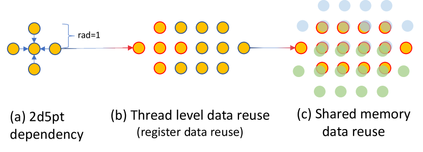
Figure 1. Spacial Blocking, using 2D 5-point Jacobian (2d5pt) stencil as an example

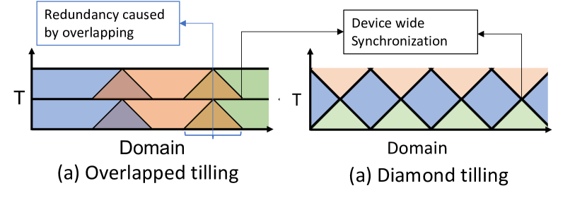
Figure 2. Temporal Blocking

Listing 1: Pseudocode for 1D 3-Point Jacobian Stencil

⬇

1for(int i=0; i<N; i++)

2 out[i]=a*in[i-1]+b*in[i]+c*in[i+1];

Listing 2: Pseudocode for 2D 5-Point Jacobian Stencil

⬇

1for(int i=0; i<N; i++)

2 for(int j=0; j<M; j++)

3 out[i][j]=a*in[i-1][j]+b*in[i][j]+c*in[i+1][j]

4 +d*in[i][j-1]]+e*in[i][j+1];

Listing 3: Pseudocode for 3D 7-Point Jacobian Stencil

⬇

1for(int i=0; i<N; i++)

2 for(int j=0; j<M; j++)

3 for(int k=0; k<L; k++){

4 out[i][j][k]= a*in[i-1][j] [k];

5 out[i][j][k]+=b*in[i] [j] [k];

6 out[i][j][k]+=c*in[i+1][j] [k];

7 out[i][j][k]+=d*in[i] [j-1][k];

8 out[i][j][k]+=e*in[i] [j+1][k];

9 out[i][j][k]+=f*in[i] [j] [k-1];

10 out[i][j][k]+=g*in[i] [j] [k+1];}

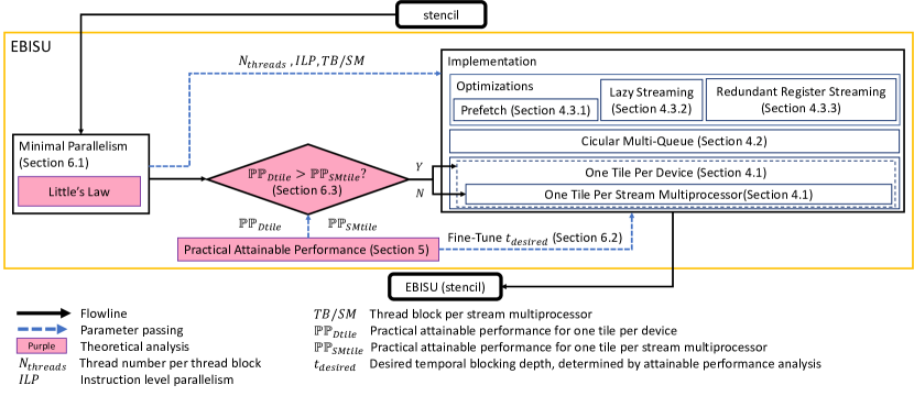
Figure 3. Overview of EBISU.

2. Background

2.1. Stencils

Stencils are characterized by their memory access patterns. We present the pseudo code for the 1D 3-Point, 2D 5-Point and 3D-7-Point Jacobian Stencil in Listing 1, Listing 2, and Listing 3 respectively. We use a 2D Jacobian 5-point (2d5pt) stencil as an example. Figure 1.a illustrates the neighborhood dependencies of the 2d5pt stencil. In order to compute one point, the four adjacent points are necessary. Two blocking methods are widely used to optimize iterative stencils for data locality:

2.1.1. Spatial Blocking

In spatial blocking on GPUs, thread (blocks) load a single tile of the domain to its local memory to improve the data locality among adjacent locations (Irigoin and Triolet, 1988; Wolfe, 1989). The local memory can be registers (Zhao et al., 2019; Chen et al., 2019)(Figure 1.b) and scratchpad memory (Maruyama and Aoki, 2014; Rawat et al., 2019)(Figure 1.c). However, halo layer(s) are still unavoidable.

2.1.2. Temporal Blocking

In iterative stencils, each time step depends on the result of the previous time step. An alternative optimization is to to combine several time steps to expose temporal locality  (Matsumura et al., 2020; Rawat et al., 2016). In this case, the temporal dependency is resolved by overlapped tilling (Holewinski et al., 2012; Meng and Skadron, 2009; Rawat et al., 2015) (Figure 2.a) or by applying complex geometry (Grosser et al., 2013; Muranushi and Makino, 2015) (Figure 2.b, diamond tiling (Grosser et al., 2014b; Bondhugula et al., 2017) as an example). The main short-coming of overlapped tiling is redundant computation, while the main disadvantage of complex geometry is an adverse effects on cache hits (Malas et al., 2015). Additionally, complex geometry is penalized by the device-wide synchronization necessary to ensure that the result is updated in the global memory.

2.1.3. N.5-D Temporal Blocking

N.5-D blocking (Matsumura et al., 2020; Rawat et al., 2018b; Nguyen et al., 2010) is a combination of spatial blocking and overlapped temporal blocking (Nguyen et al., 2010). Take 3.5-D temporal blocking as an example. We do spatial tiling in the X and Y dimensions, and then stream in the Z dimension (2.5-D spatial blocking). As we stream over the Z dimension, each XY plane would conduct a series of temporal steps (1-D temporal blocking). This method reduces the overhead of redundant computations in an overlapped temporal blocking schema.

2.2. GPU Architecture

2.2.1. CUDA Programming Model

The CUDA programming model includes: the base execution unit, thread; 32 threads grouped into a block of schedule units, warp; Several warps grouped together into a thread block unit; and thread block units can be grouped into a grid. When mapping the programming model to the GPU architecture, the CUDA driver maps the thread block to a Stream Multiprocessor (SM) and grids to a GPU device. The mapping abides by the rules of dividing the resources among the threads. For example, at most 8 thread blocks and at most 2048 threads can reside concurrently on a stream multiprocessor. Also, the total number of registers and shared memory in a stream multiprocessor also limits the number of thread block that can run concurrently.

2.2.2. Explicit Synchronization

Nvidia introduced cooperative group APIs (CUDA, 2022) to provide a hierarchical of synchronizations in addition to thread block synchronization from P100 (2016). Among them, the new grid level synchronization provides additional choice for program. Zhang et. al. (Zhang et al., 2020) shows that latencies of these APIs are acceptable that would allow practical use.

2.2.3. Asynchronous Shared Memory Copy.

A100 (2020) further introduced APIs (CUDA, 2022) to copy data from global memory to shared memory, without blocking. Martin et al. (Svedin et al., 2021) demonstrated that this API benefits low-arithmetic intensity kernels.

3. EBISU: High Performance Temporal Blocking at Low Occupancy

In this section we give an overview of our temporal blocking method: EBISU (Figure 3 gives an overview) The design of EBISU follows two main principles: minimal parallelism that would saturate the device (the Minimal Parallelism step in Figure 3), and scalability in using resources (the Implementation step in Figure 3). Additionally, EBISU relies on a comprehensive analysis for implementation decisions (the pink steps in Figure 3).

3.1. Saturating the Device at Minimal Parallelism

In EBISU we first tune the parallelism exposed in the kernel to find the minimal combination of occupancy and instruction level parallelism that would saturate the device. The minimal occupancy that we aim for in this paper is $12.5\%$ since further reducing the occupancy for memory-bound codes can start to regress the performance (Nvidia, 2022b). We aim to minimize resources used for increasing the locality. We use Little’s Law to identify the minimum parallelism (occupancy) in the code (discussed in Section 6.1). We point out that readers can also rely on auto-tuning tools to empirically figure out the minimal parallelism (van Werkhoven, 2019; Shende and Malony, 2006; Rawat et al., 2019).

3.2. Scaling the Use of Resources

Despite the relatively large amount on-chip resources, there is a lack in design principles that are able to scale up to take advantage of the large on-chip resources in temporal blocking. We thereby build on a set of existing optimizations to drive a resource-scalable scheme for increasing locality (Section 4).

3.3. Implementation Decisions

We base the decision for implementing EBISU on our analysis for the practical attainable performance (Section 5). The main utility of this analysis is to decide whether to implement a device tile (Section 6.3), and the parameterization of spatial and temporal blocking (Section 6.4)).

3.4. Fine-Tuning

After identifying the ideal tiling scheme and parameterization, implementation, we fine-tune the kernel to extract additional performance. For instance, we tune the temporal blocking depth (Section 6.2).

4. Efficiently Scaling the Use of Resources

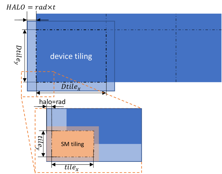
Figure 4. 2D Spatial tiling at the GPU device level.

Listing 4: Pseudocode for 2D 5-Point Jacobian stencil device level spatial tiling.

⬇

1void __global__ void device_2d5pt(…){…

2 //data is loaded from on-chip memory ocm_in

3 //store data to ocm_out

4 //ocm range tile_x, and tile_y;

5 for(int s=0; s<t; s++){

6 for(int l_y=0; l_y<tile_y; l_y+=1){

7 for(int l_x=0; l_x<tile_x; l_x+=blockDim.x){

8 ocm_out[i][j]=a*ocm_in[i-1][j]+b*ocm_in[i][j]

9 +c*ocm_in[i+1][j]+d*ocm_in[i][j-1]

10 +e*ocm_in[i][j+1];}

11 __syncthreads();

12 push_halo_to_neighbor(ocm_out[][],global_memory);

13 grid.sync();

14 swap(ocm_out,ocm_in);

15 pull_halo_from_neighbor(ocm_in[][],global_memory);

16 __syncthreads();

17 }

18…}

4.1. One Tile At A Time

Beyond the point where the GPU becomes saturated, the workload will inevitably be serialized. We intentionally introduce a method to serialize the execution of tiles, where each individual tile becomes large enough to saturate the GPU. We call this device tiling. Alternatively, we can use tiles that are executed in parallel, yet each tile individually saturates a single streaming multiprocessor. We call this SM tiling.

In device tiling, we tile the domain such that a single tile can scale up to use the entire on-chip memory capacity of the GPU. Next, we let the tile reside in the on-chip memory while updating the cells for a sufficient number of time steps to amortize the initial loading and final storing overheads. We then store the final result for the tile on the device, and then we move to the next tile, i.e., the entire GPU is dedicated to computing only one single tile at any given time. Figure 4 shows how we do spatial tiling at the device level. We assume $tile_{x}\times tile_{y}$ to be the thread block tile configuration and $Dtile_{x}\times Dtile_{y}$ to be the device tile configuration. Thus, $(tile_{x}+halo\cdot 2)\times(tile_{y}+halo\cdot 2)$ is the total on-chip memory consumed at the stream multiprocessor level. $(Dtile_{x}+HALO\cdot 2)\times(Dtile_{y}+HALO\cdot 2)$ is the total on-chip memory consumed at the device level, where $HALO=rad\cdot t$. Additionally, figure 1.c shows the dependency between thread blocks that we need to resolve. We use the bulk synchronous parallel (BSP) model to exchange the halo region and CUDA’s grid level barrier for synchronization. We transpose the halo region that originally did not coalesce to reduce the memory transactions. Note that device tiling is an additional layer on top of SM tiling. Figure 4 shows an example of 2D spatial tiling at device level, and Listing 4 presents the pseudocode of a 2D 5-point Jacobian stencil with device level spatial tiling.

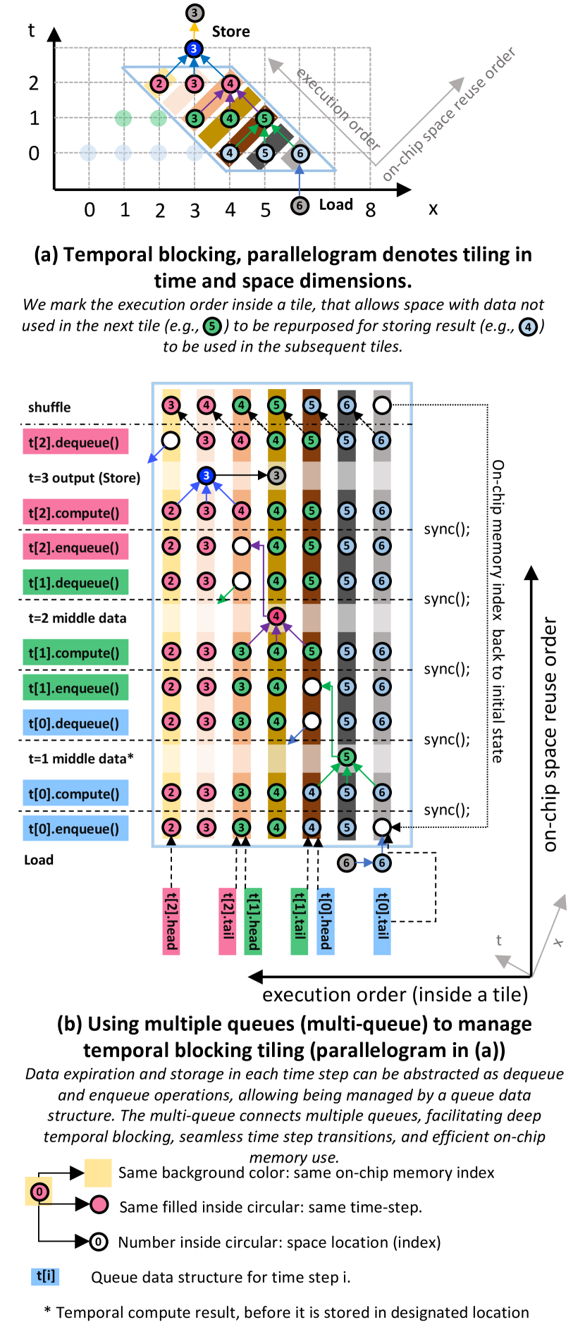
Figure 5. The multi-queue data structure enables efficient temporal blocking tiling: a 1D 3-Point Jacobian stencil with a depth of 3 as an example. Figure (a) illustrates streaming with a parallelogram that we process in Figure (b). Figure (b) illustrate how queue data structure can enhance the processing of the tiling depicted in Figure (a). The execution order and data reuse are marked in both figures.

Listing 5: Pseudocode for applying naive multi-queue data structure to a 1D 3-Point Jacobian stencil with temporal blocking depth of 3.

⬇

1struct Queue {

2 REAL* d; //data array

3 index tl; //tail

4 index hd; //head

5 Queue(REAL*data,index head,index tail):

6 d(data),hd(head),tl(tail){}

7 REAL dequeue(){}//Automatically accomplished by shuffle

8 void enqueue(REAL input){d[tl]=input;}

9 REAL compute()

10 {return a*d[hd]+b*d[hd+1]+c*d[hd+2];}//1d3pt stencil

11};

12template<int depth>

13struct MultiQueue{//Multi-queue data structure

14 REAL* d; //data array

15 index hds[depth]; //head of queues

16 index r;//range of multi-queue

17 index q_r;//range of single queue, reserved for lazy streaming

18 MultiQueue(REAL*data, index range, index queue_range):

19 d(data),r(range),q_r(queue_range)

20 {for(t=0; t<depth; t++)hds[t]=queue_range-q_r*s;}

21 MultiQueue(REAL*data, index range):

22 MultiQueue(data,range,2){}

23 Queue operator[](int t) {return Queue(d,hds[t],hds[t]+q_r);}

24 void shuffle(){//default, move data

25 sync();

26 for(int i=0; i<r-1; i++)d[i]=d[i+1];

27 sync();

28 }

29}

30#define RANGE (7)

31__global__ void 1d3ptstencil(REAL* input, REAL* output,…){…

32 REAL buffer[RANGE];

33 MultiQueue t<3>(buffer, RANGE, 2);

34 for(…){…

35 t[0].enqueue(Load(input));

36 sync();

37 for(s=0; s<3-1; s++){

38 tmp=t[s].compute();

39 sync();

40 t[s+1].enqueue(tmp);

41 //Do t[s].dequeue() t[s+1].enqueue()

42 sync();

43 }

44 Store(ouput[],t[3-1].compute()…);

45 …

46 t.shuffle();//shuffle head and tail index for next tiling

47 …}

48}

Listing 6: Pseudocode for applying circular multi-queue data structure, which inhirits the structure described in Listing 5.

⬇

1index mod(index a,index r){return (r&(r-1))==0)?a&(r-1):a%r;}

2struct Circular_Queue: public Queue {

3//Circular queue inhirit from queue

4 index r;

5 Circular_Queue(REAL*data,index head,index tail,index range,):

6 d(data),hd(head),r(range),tl(tail){}

7 REAL compute()//override 1d3pt stencil

8 {return a*d[hd]+b*d[mod((hd+1),r)]+c*d[mod((hd+2),r)];}

9};

10template<int depth>//Circular multi-queue inhirit from multi-queue

11struct Circular_MultiQueue: public MultiQueue<depth>{

12 Circular_MultiQueue(REAL*data, index range)

13 :Multi-queue<depth>(data,range){}

14 Circular_MultiQueue(REAL*dat, index ran, index q_ran)

15 :MultiQueue<depth>(dat,ran,q_ran){}

16 Circular_Queue operator[](int t)

17 {return Circular_Queue(d,hds[t],mod(hds[t]+2,r),r);}

18 void shuffle(){//Override shuffle for computing address schema

19 for(int i=0; i<r; i++)hds[i]=mod((hds[i]+1),r);

20 }

21}

22#define RANGE (8)

23…//kernel code unchange

4.2. Circular Multi-Queue

EBISU aims to scale up resource usage. One way to achieve this goal is to scale up to very deep temporal blocking. In this section, we introduce a simple data structure that enables the efficient management of very deep temporal blocking: namely, circular multi-queue. We elaborate on our design by first introducing multi-queue for streaming (Section 4.2.1), and then we describe the implementation of the circular multi-queue (Section 4.2.2).

4.2.1. Multi-Queue

We use the 1D 3-Point Jacobian stencil (Listing 1) to illustrate our implementation. Streaming is a typical method to implement temporal blocking. Figure 5.a demonstrates an example of streaming. The parallelogram in the figure represents the tiling in time and spatial dimensions that we process in Figure 5.b. The process of each time step can be abstracted as two functions: enqueue and dequeue, which are standard methods in a queue data structure. We additionally add compute for stencil computation. As such, we manage each time step with a queue data structure. Next, we link queues in different time steps together, to become a multi-queue data structure. The data structure description and the pseudocode for multi-queue is in Listing 5.

Multi-queue facilitates seamless transitions between time steps. The dequeue operation (data expiration) for the current time step runs concurrently with the enqueue operation for the next time step. After the execution of a single tile, we reset the multi-queue to its initial state - a process we refer to as ’shuffle’. A standard method of conducting a shuffle involves shifting values to their designated locations, as demonstrated in lines 24-27 of Listing 5.

It is important to note that although we base our analysis on a 1D stencil example in this section, it can be simply extended to 2D or 3D stencils by replacing the 1D circular points (domain cells) in Figure 5 to 1D lines (corresponding to 2D stencils) or 2D planes (corresponding to 3D stencils), or even the device tiles discussed in Section 4.1. In the device tiling situation, the sync(); function should be replaced by device (grid) level synchronization. Additionally, we can trade the concurrently processed domain cells for additional instruction level parallelism (ILP), which might be required by the parallelism setting (discussed in Section 6.1).

4.2.2. Circular Multi-Queue

We further adapt the multi-queue to be circular. We wrap the tail of time step 0 and the head of the deepest time step together. We detail the implementation of different circular multi-queue we use as follows:

Shifting Addresses: In this scheme, we only copy the index to the same place after processing a tile (at the ’shuffle step’).

Computing Address: Shifting addresses is the simplest way to manage the circular data structure. However, shifting can create a long chain of dependencies as the address range increases. An alternative solution is to compute the target address (Listing 6 line 7-8.). The modulo operation is one of the solutions; however, this operator is time consuming. Instead, we extend the ring index to be $range=2^{n},n\in\mathbb{Z}^{+}$. In this case, we have $index\%range=index\&(range-1)$. This consumes additional space (Listing 6 line 22).

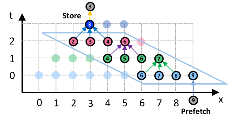
Figure 6. Lazy streaming for temporal blocking. 1D 3-Point Jacobian stencil with depth=3 as an example. Notations are the same as Figure 5.

Listing 7: Pseudocode for applying lazy streaming to a 1D
3-Point Jacobian stencil with temporal blocking depth of 3.

⬇

1//Lazy streaming kernel code

2__global__ void 1d3ptstencil_lz(REAL* input, REAL* output,…){…

3 REAL buffer[16];//more space for buffering

4 Circular_MultiQueue t<3>(buffer, 16, 3);

5 for(…){…

6 t[0].enqueue(Load(input));//prefetch

7 for(s=0; s<3-1; s++){

8 tmp=t[s].compute();

9 t[s+1].enqueue(tmp);

10 }

11 Store(ouput[],t[3-1].compute()…);

12 …

13 t.shuffle();//shuffle head and tail index for next tiling

14 sync();//One sync per tile

15 …

16 }

17}

4.3. Optimizations

4.3.1. Prefetching

Prefetching is a well-documented optimization. Readers can refer to (Rawat et al., 2019) for hints. The new asynchronous shared memory copy API offers another approach for prefetching, with a trade-off of requiring additional shared memory space for buffering.

4.3.2. Lazy Streaming

The naive implementation showed in Figure 5 and Listing 5 clearly suffers from the overhead of frequent synchronization. We propose lazy streaming to alleviate this type of overhead. The basic idea is that we delay the processing of a domain cell until all domain cells required to update the current cell are already updated. Otherwise, we would pack the planes that include the current domain cell and cache it in on-chip memory. As Figure 6 shows, the computation of location 3 is postponed until the three points of the previous time steps have been updated.

The benefit of using lazy streaming is not significant in 1D stencils. In 2D or 3D stencils, we replace the points in Figure 6 with 1D or 2D planes for 2D or 3D stencils. The planes usually involve inter-thread dependency, which makes synchronizations unavoidable (warp shuffle when using registers for locality (Chen et al., 2019, 2018) or thread block synchronization when using shared memory for locality (Maruyama and Aoki, 2014)). when applying device tiling (Section 4.1), device (grid) level synchronization becomes unavoidable, and it has higher overhead in comparison to thread block synchronizations. As illustrated in Listing 7, lazy streaming can ideally reduce the synchronization to one synchronization per tile. The benefit of lazy streaming comes from the number of synchronization it reduced.

It’s worth noting that double-buffering (Matsumura et al., 2020; Rawat et al., 2018b) can be viewed as a special case of lazy streaming when only a single queue evolved.

4.3.3. Redundant Register Streaming

The above discussions, which do not specify the on-chip memory type, can apply to both shared memory-based and register based implementations. However, there is one exception: the circular multi-queue cannot be implemented with register arrays since register addresses cannot be determined at compile time.

At low occupancy, we obtain a large number of registers and shared memory per thread. Therefore, by reducing the occupancy, we can afford to redundantly store intermediate data in both the registers and the shared memory. Streaming w/ caching in shared memory is discussed in STENCILGEN (Rawat et al., 2018b). Streaming w/ caching in the registers is discussed in AN5D (Matsumura et al., 2020). We benefit from both components by caching in both shared memory and registers. We can reduce shared memory access times to their minimum by using registers first (in comparison to AN5D) and reducing the necessary synchronizations when using only shared memory (in comparison to STENCILGEN). Additionally, due to data being mostly redundant, we can tune to reduce resource usage in either part of registers or shared memory to reduce the resource burden.

5. Practical Attainable Performance

In this section, we analyze the practical attainable performance of temporal blocking by incorporating an the overhead analysis (we derive valid proportion $\mathbb{V}$ from overhead analysis in Section 5.2) to a roofline-like model (Ofenbeck et al., 2014; Kim et al., 2011) that predicts the attainable performance ($\mathbb{P}$ in Section 5.1). We project the practical attainable performance $\mathbb{PP}$ as:

(1) $$\footnotesize\mathbb{PP}=\mathbb{P}\times{\mathbb{V}}$$

The model proposed in this section serves as a guide for implementation design choices in Section 6.

5.1. Attainable Performance

We use the giga-cells updated per second (GCells/s) as the metric for stencil performance (Matsumura et al., 2020; Chen et al., 2019). We consider three pressure points in a stencil kernel: double precision ALUs, cache bandwidth (i.e., shared memory bandwidth in this paper), and device memory bandwidth (GPU global memory in this paper). Note that registers could also be a pressure point in extreme cases of very high order stencils (outside the scope of this paper).

Assuming that the global memory bandwidth is $\mathbb{B}_{gm}$, the shared memory bandwidth is $\mathbb{B}_{sm}$, and the compute speed is $\mathbb{THR}_{cmp}$, the total access time is $\mathbb{A}_{gm}$ and $\mathbb{A}_{sm}$ for global memory and shared memory, respectively. The total amount of computation is $\mathbb{A}_{cmp}$. The memory access time per cell is ${a}_{gm}$ and ${a}_{sm}$ for global memory and shared memory, respectively; flops per cell is ${a}_{cmp}$. The total number of cells in the domain of interest is $\mathbb{D}_{gm}$, $\mathbb{D}_{sm}$ and $\mathbb{D}_{gm}$ for global memory, shared memory, and computation, respectively. The size of the cell (in Bytes) per cell is $\mathbb{S}_{Cell}$. We can compute the runtime of using each component to be:

(2) $$\footnotesize\begin{split}\mathbb{T}_{gm}&=\frac{\mathbb{A}_{gm}}{\mathbb{B}_{gm}}\times\mathbb{S}_{Cell}=\frac{{a}_{gm}\times\mathbb{D}_{gm}}{\mathbb{B}_{gm}}\times\mathbb{S}_{Cell}\end{split}$$

(3) $$\footnotesize\begin{split}\mathbb{T}_{sm}&=\frac{\mathbb{A}_{sm}\times t}{\mathbb{B}_{sm}}\times\mathbb{S}_{Cell}=\frac{{a}_{sm}\times\mathbb{D}_{sm}\times t}{\mathbb{B}_{sm}}\times\mathbb{S}_{Cell}\end{split}$$

(4) $$\footnotesize\begin{split}\mathbb{T}_{com}&=\frac{\mathbb{A}_{cmp}\times t}{\mathbb{THR}_{cmp}}=\frac{{a}_{cmp}\times\mathbb{D}_{cmp}\times t}{\mathbb{THR}_{cmp}}\\ \end{split}$$

The total runtime of the stencil is projected as:

(5) $$\footnotesize\mathbb{T}_{stencil}=\max(\mathbb{T}_{gm},\mathbb{T}_{sm},\mathbb{T}_{cmp})$$

The component $c$ is the bottleneck if it satisfies:

(6) $$\footnotesize\mathbb{T}_{c}=\mathbb{T}_{stencil}$$

We project the attainable performance $\mathbb{P}$ as:

(7) $$\footnotesize\mathbb{P}=\frac{\mathbb{D}_{all}\times{t}}{\mathbb{T}_{stencil}}$$

Normally, we consider $\mathbb{D}_{all}=\mathbb{D}_{sm}=\mathbb{D}_{gm}=\mathbb{D}_{cmp}$. However, this is a case-by-case factor that depends on the implementation, i.e., when applying device tiling $\mathbb{D}_{gm}\neq\mathbb{D}_{sm}$.

5.2. Overheads

In this section, we discuss the overheads of different spatial blocking methods used in this paper:

5.2.1. SM Tiling

The main overhead of SM tiling is related to redundant computation in halo. Only a portion of the computation is valid. This valid portion is related to both the spatial and temporal block sizes and the radius of the stencil. In 2D stencils, we have:

(8) $$\footnotesize\mathbb{V}=\frac{tile_{x}-t\times rad}{tile_{x}}$$

In 3D stencils, we have:

(9) $$\footnotesize\mathbb{V}_{SMtile}=\frac{(tile_{x}-t\times rad)\times(tile_{y}-t\times rad)}{tile_{x}\times tile_{y}}$$

Accordingly, we have:

(10) $$\footnotesize\mathbb{PP}_{SMtile}=\mathbb{V}_{SMtile}\times\mathbb{P}$$

5.2.2. Device Tiling

The main overhead of the device level tiling is related to the overhead of synchronization. Only a portion of the runtime is valid. The valid portion depends on the runtime of the stencil ($\mathbb{T}_{stencil}$), the time required for device level synchronization ($\mathbb{T}_{Dsync}$) and the number of synchronization times per tile $n$ (applying lazy streaming (Section 4.3.2) reduces $n$ to 1):

(11) $$\footnotesize\mathbb{V}_{Dtile}=\frac{\mathbb{T}_{stencil}}{\mathbb{T}_{stencil}+\mathbb{T}_{Dsync}\times n}$$

Accordingly, we have:

(12) $$\footnotesize\mathbb{PP}_{Dtile}=\mathbb{V}_{Dtile}\times\mathbb{P}$$

To quantify the overhead, we followed the research of Zhang et al. (Zhang et al., 2020) to test the overheads. The device (grid) level synchronization overhead in A100 is : $\mathbb{T}_{Dsync}=1.2us$.

Table 1. Design choices for EBISU.

Type	Parallelism Combination	SM Tiling	Device Tiling	Temporal Blocking Strategy	Circular Multi-Queue
	($N_{threads}\times ILP$)	($tile_{x}\times tile_{y}$)
2D stencils	$256\times 4$	$256\times 4$	–	Deep enough to shift the bottleneck	Compute
3D stencils	$256\times 4$	$32\times 32$	$(12\times 6)$	As deep as possible	Shifting

6. EBISU: Analysis of Design Choices

In this section, we provide a comprehensive analysis to justify our design choices. The analysis is targeted at the A100 GPU, while it can be generalized to any GPU platform by adjusting the model parameters (Table 1 summarizes our findings on design choices).

We use 2D 5-Point (Listing 2) to represent 2D stencils, and 3D 7-Point (Listing 3) to represent 3D stencils for the discussions in this section. Table 2 shows the detailed parameters of both stencils.

6.1. Minimum Necessary Parallelism

The analysis of this section is an extension of Volkov’s work on low occupancy at high performance (Volkov, 2010). We also generalize the analysis by building on Little’s law. Little’s saw uses latency $\mathbb{L}$ and throughput $\mathbb{THR}$ to infer the concurrency $\mathbb{C}$ of the given hardware:

(13) $$\footnotesize\mathbb{C}=\mathbb{L}\times\mathbb{THR}$$

The latency $\mathbb{L}$ of an instruction can be gathered by common microbenchmarks (Wong et al., 2010; Mei and Chu, 2016). The throughput $\mathbb{THR}$ of instructions is available in Nvidia’s CUDA programming guide (CUDA, 2022) and documents (Nvidia, 2022b).

As long as the parallelism $\mathbb{PAR}$ provided by the code is larger than the concurrency provided by the hardware, we consider that the code saturates the hardware:

(14) $$\footnotesize\mathbb{PAR}\geq\mathbb{C}$$

There are two ways of providing parallelism: number of threads ($N_{threads}$) and Instruction Level Parallelism ($ILP$). So, we have:

(15) $$\footnotesize\mathbb{PAR}={N_{threads}}\times{ILP}$$

Unlike Volkov’s analysis, instead of maximizing the parallelism with the combination of $ILP$ and $N_{threads}$, we aim to find a minimal combination of $N_{threads}$ and $ILP$ that saturates the device:

(16) $$\footnotesize{N_{threads}}\times{ILP}=\mathbb{PAR}\geq\mathbb{C}=\mathbb{L}\times\mathbb{THR}$$

To maintain a certain level of parallelism, we can reduce the occupancy ($N_{threads}$) and increase $ILP$ simultaneously. We reduce the occupancy to the point that it will not increase the resources per thread block. In the current generation of GPUs (A100), reducing the occupancy of memory-bound kernels to less than $12.5\%$ will not increase the available register per thread (CUDA, 2022). So, we set our aim conservatively at $Occupancy=12.5\%$ or $N_{threads}=256$.

In this research, we focus on double precision global memory access, shared memory access, and DFMA, all of which are the basic operations in stencil computation. Based on our experimentation, $ILP=4$ and $Occupancy=12.5\%$ ($N_{threads}=256$) provide enough parallelism for all three operations. We set this as a basic parallelism combination for our implementation. Note that the numbers above may vary for other GPUs, yet the analysis still holds.

6.2. Desired Depth

We use the attainable performance analysis (Section 5.1) to infer the desired depth. We aim at determining a sufficiently deep temporal blocking size to shift the bottleneck.

In this study, we are less concerned with whether the bottleneck shifts to computation or cache bandwidth. To simplify the discussion, we assume that the optimization goal is shifting the bottleneck from global memory to shared memory. This assumption is true for most of the star-shaped stencils (Matsumura et al., 2020). Accordingly, we have:

(17) $$\footnotesize\frac{{a}_{sm}\times t}{\mathbb{B}_{sm}}\times{\mathbb{D}_{sm}}\geq\frac{{a}_{gm}}{\mathbb{B}_{gm}}\times\mathbb{D}_{gm}$$

6.2.1. Case Study: 2D 5-Point Jacobian Stencil (representing stencils w/o device tiling)

Ideally, we have $\mathbb{D}_{sm}=\mathbb{D}_{gm}$. In A100, $\mathbb{B}_{gm}=1555$ GB/s, $\mathbb{B}_{sm}=19.49$ TB/s. In our 2D 5-point implementation, $\mathbf{a}_{gm}=2$ (assuming perfect caching), $\mathbf{a}_{sm}=4$. According to Equation 17, we have $t\geq 6.3$. In $t=7$, we measured the performance of $440$ GCells/s. We can fine-tune to achieve slightly better performance at $t=12$, where we measured $482$ GCells/s. There is only a $10\%$ difference in performance. The slight inaccuracy might come from the fact that, on average, the global memory accesses per data point is not perfectly cached.

6.2.2. Case Study: 3D 7-Point Jacobian Stencil (representing stencils w/ device tiling)

In device tiling 3D 7-point stencil, $\mathbb{D}_{gm}$ must also include the halo region between thread blocks. As such, we have:

(18) $$\footnotesize\mathbb{D}_{gm}=(tile_{x}\times tile_{y})+(tile_{x}+tile_{y})\times 2\times t\times rad$$

We intend to determine a $t$ that satisfies:

(19) $$\footnotesize\frac{{a}_{sm}\times\mathbb{D}_{sm}\times t}{\mathbb{B}_{sm}}>\frac{{a}_{gm}\times\mathbb{D}_{gm}}{\mathbb{B}_{gm}}$$

We assume that $tile_{x}=tile_{y}=32$. We have $a_{sm}=4.5$, $a_{gm}=2$. So we can get $t>18.34$. In this situation, the on-chip memory per thread block desired for EBISU is $352$ KB, which exceeds the capacity of A100 ($164$ KB).

6.3. Device Tiling or SM Tiling?

Device tiling trades redundant computation for device level synchronization. In this section, we focus on: in EBISU, the performance implications of using one single tile per device (w/ device level synchronization). By comparing the practical attainable performance with the version that is not using one single tile per device (w/o device level synchronization).

6.3.1. Case Study: 2D 5-Point Jacobian Stencil

In 2d5pt, we have $\mathbb{T}_{stencil}=\mathbb{T}_{sm}$ for the overlapped tilling and the device level tiling. We simplify the discussion by defining a valid proportion $\mathbb{V}$, i.e., the updated output after excluding the halo. The higher the valid proportion, the higher the performance $\mathbb{P}$. In overlapped tiling, for 2d5pt we have $t=7$ (Section 6.2.1) and $rad=1$. So $\mathbb{V}_{SMtile}\approx 95\%$

For device level tiling, we can go as deep as $t=15$. So, we have: $\mathbb{T}_{sm}=2.05us$. Because $\mathbb{T}_{Dsync}=1.2us$. Accordingly, we have $\mathbb{V}_{Dtile}={\mathbb{T}_{sm}}/{(\mathbb{T}_{sm}+\mathbb{T}_{Dsync})}\approx 63\%$.

So, we have: $\mathbb{V}_{Dtile}\ll\mathbb{V}_{SMtile}$.

For 2D stencils of other shapes, we get:

(20) $$\footnotesize\mathbb{PP}_{Dtile}(2D)\ll\mathbb{PP}_{SMtile}(2D)$$

As a result, in 2D stencils, the overhead of thread block level overlapped tiling is negligible, making device tiling less beneficial. This result stands true for all 2D stencils we studied in A100.

6.3.2. Case Study: 3D 7-Point Jacobian Stencils

In 3d7pt, we cannot shift the bottleneck to shared memory in overlapped (within acceptable overhead) or device tiling. We need to compare the Practical Attainable Performance in both cases to judge.

We have $\mathbb{V}_{SMtile}={(34-2\times rad\times t)^{2}}/{34^{2}}$. In 3d7pt, we have $rad=1$, $t=3$, $\mathbb{V}_{SMtile}\approx 77\%$. In $t=3$, we have $\mathbb{P}_{SMtile}=292$ GCells/s, and $\mathbb{PP}_{SMtile}\approx 225$ GCells/s.

On the other hand, for device tiling, we can go as deep as $t=8$, so we have $\mathbb{L}(gm)=2.42$ . Because $\mathbb{T}_{Dsync}=1.2$ us. So, $\mathbb{V}_{Dtile}\approx 67\%$ GCells/s. In $t=8$ we have $\mathbb{P}_{Dtile}=365$ GCells/s. Accordingly, we have $\mathbb{PP}_{Dtile}\approx 244$ GCells/s.

So, we have: $\mathbb{PP}_{Dtile}>\mathbb{PP}_{SMtile}$ on a 3d7pt stencil.

We measured, for instance, $151$ GCells/s for w/o device tiling and $197$ GCells/s for w/ device tiling. The experiment results is consistent with the analysis (for 3D stencils of other shapes as well):

(21) $$\footnotesize\mathbb{PP}_{Dtile}(3D)>\mathbb{PP}_{SMtile}(3D)$$

As a result, for 3D stencils, the overhead of thread block level overlapped tiling is so significant that it prohibits the temporal blocking implementation from going deeper. This result stands true for all 3D stencils we studied in A100.

Based on the analyses above, in EBISU, we only implement device tiling for 3D stencils. The analysis in the following section is built on top of this decision.

6.4. Deeper or Wider?

As the capacity of on-chip memory is limited, there is a trade-off between increasing the width of spatial blocking and increasing the depth of temporal blocking. In this section, we discuss our heuristic for we use for parameter selection in EBISU.

6.4.1. Case Study: 2D 5-Point Jacobian Stencil

Firstly, as Section 6.3.1 showed, the overhead of 2D 5-Point Jacobian Stencil is negligible. Additionally, according to Section 6.2.1, in theory, at depth $t=7$, we shift the bottleneck from global memory to shared memory.

As such, after the bottleneck is shifted, we aim at wider spatial blocking to reduce the overhead of overlapped tilling as is discussed in Section 5.2.1. Yet, we still need to consider the implementation simplicity. For example, we choose a tiling of size $tile_{x}=256$ instead of $tile_{x}=328$, since the latter is hard to implement in CUDA. .

6.4.2. Case Study: 3D 7-Point Jacobian Stencil

For simplicity, we assume that the very first plane loaded and the last plane stored have already been amortized. Then, for global memory access, we only focus on the halo region. According to Equation 17, we have:

(22) $$\footnotesize\frac{tile_{x}\times tile_{y}\times{a}_{sm}}{\mathbb{B}_{sm}}>\frac{(tile_{x}+tile_{y})\times 2\times{a}_{gm}\times rad}{\mathbb{B}_{gm}}$$

We assume that $tile_{y}=tile_{x}$. So, we can get:

(23) $$\footnotesize tile_{y}=tile_{x}>{\frac{4\times{a}_{gm}\times\mathbb{B}_{sm}}{{a}_{sm}\times\mathbb{B}_{gm}}}\times rad$$

In our 3d7pt implementation, ${a}_{gm}=2$, ${a}_{sm}=4.5$. We have $tile_{y}=tile_{x}\geq 22.3$. For implementation convenience, we use $32\times 32$ (also fitted to the Minimal Necessary Parallelism that saturates the device as Section 6.1 discussed). As such, after the spatial tiling is large enough for overlapping halo region, we then run the temporal blocking as deep as possible to amortize the overhead of using device (grid) level synchronization.

7. Evaluation

Table 2. Stencil benchmarks. Readers can refers to  (Rawat et al., 2018b; Matsumura et al., 2020) for details description. We also include ideal shared memory access times per cell, $a_{sm}$, when applying redundant register streaming (w/ RST) and without it (w/o RST) in the table.

Stencil	Domain Size	$a_{sm}$	$a_{sm}$
[Order, FLOPs/Cell]		w/o RST	w/ RST
j2d5pt [1,10]	$8352^{2}$	6	4
j2d9pt [2,18]	$8064^{2}$	10	6
j2d9pt-gol [1,18]	$8784^{2}$	10	4
j2d25pt (gaussian) [2,25]	$8640^{2}$	26	6
j3d7pt (heat) [1,14]	$2560\times 288\times 384$	8	4.5
j3d13pt [2,26]	$2560\times 288\times 384$	14	7
j3d17pt [1,34]	$2560\times 288\times 384$	18	5.5
j3d27pt [1,54]	$2560\times 288\times 384$	28	5.5
poisson [1,38]	$2560\times 288\times 384$	20	5.5

Table 3. Depth of temporal blocking for each stencil implementations in this evaluation.

Type	STENCILGEN	AN5D	DRSTENCIL	ARTEMIS	EBISU
j2d5pt	4	10	3	12	12
j2d9pt	4	5	2	6	8
j2d9pt-gol	4	7	2	6	6
j2d25pt	2	5	2	3	4
j3d7pt	4	6	3	3	8
j3d13pt	2	4	2	1	5
j3d17pt	2	3	2	2	6
j3d27pt	2	3	-	2	5
poisson	4	3	2	2	6

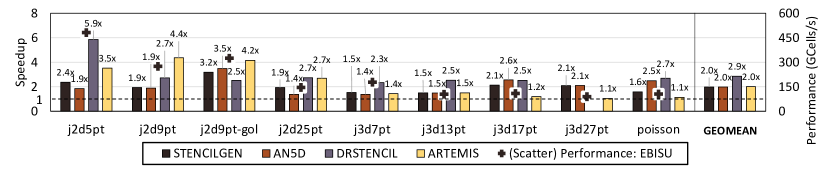
Figure 7. Speedup of EBISU over the state-of-the-art temporal blocking implementations. We also plot the performance of EBISU (right Y-axis plotted as ’$+$’ ticks).

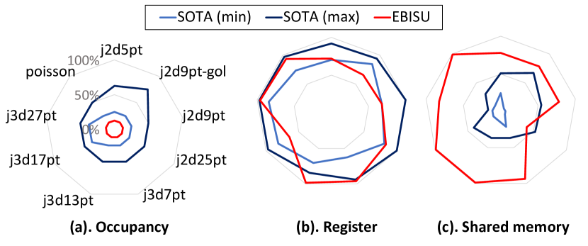
Figure 8. Percent of occupancy achieved and resources used (registers and shared memory) for EBISU and SOTA libraries among all stencil benchmarks.

We experiment on a wide range of 2D and 3D stencils (listed in Table 2). The test data are generated by STENCILGEN (Rawat et al., 2018b). We evaluate the benchmarks on an NVIDIA A100-PCIe GPU device(host CPU: Intel Xeon E5-2650).

7.1. Compile Settings of EBISU

The code is compiled with NVCC-11.5 (CUDA driver V11.5.119) and gcc-4.8.5, using flags -rdc=true -Xptxas ”-v ” -std=c++14. We only generate code for A100 architecture . ”–rdc=true” flag is necessary for enabling grid level synchronization, so we set it by default. We use c++14 features, so we add ”-std=c++14” flag. -Xptxas ”-v” is set to gather information on registers.

7.2. Evaluation Setup

7.2.1. Domain Size

We used the domain sizes listed in Table 2 for EBISU, comparable to those used in the literature (Chen et al., 2019; Bondhugula et al., 2017; Rawat et al., 2018a).

7.2.2. Warm-Up and Timing

For all experiments, we do warm-up iterations and then use GPU event APIs to measure one kernel run. We repeat this process ten times and report the peak.

7.2.3. Depth of Temporal Blocking

We only evaluate a single kernel. Therefore, the total number of time steps is equal to the depth of temporal blocking of each implementation in each stencil benchmark. We summarize the depth of temporal blocking in Table 3.

7.3. Comparing with State-Of-The-Art Implementations

We compare EBISU with the state-of-the-art temporal blocking implementations AN5D (Matsumura et al., 2020) and STENCILGEN (Rawat et al., 2018b), and the state-of-the-art auto-tuning tools ARTEMIS (Rawat et al., 2019) and DRSTENCIL (You et al., 2021).

7.3.1. Setting up State-Of-The-Art Libraries

We use the domain sizes reported by each library in the original paper (not adversely change domain sizes). We assume that the libraries can achieve reasonably good performance in the setting used in the original paper. For example, in 2D stencils, AN5D used $16384^{2}$, while STENCILGEN used $8192^{2}$. ARTEMIS did not report 2D stencils; we used the same setting as STENCILGEN. Details can be obtained from the original papers (Matsumura et al., 2020; Rawat et al., 2018b, 2019; You et al., 2021).

As for timing and warm-up. AN5D’s original code already does the warm-up, so we use the default setting. We use the same host warm-up and timer function as EBISU to test the kernel performance for STENCILGEN, ARTEMIS, and DRStencil.

The detailed settings are listed as follows:

STENCILGEN We used the codes for AD/AE appendix (Rawat, 2023b) of the original paper. We do not change anything inside the kernel.

AN5D AN5D is a code auto-generator tool. We only used the code already generated in their code (Matsumura, 2023) . We port the makefile system to A100 and iterate over all generated codes to find the one with the highest performance for each stencil benchmark. The original code did not include some stencil benchmarks we use. We use the implementations with similar memory access patterns to represent them: gaussian (box2d2r), j3d7pt (star3d1r), j3d13pt (star3d2r), j3d17pt (j3d27pt) and poisson (j3d27pt).

DRSTENCIL DRSTENCIL (You et al., 2021) is also an auto-tuning tool. We use the benchmark in the codebase (Jiang, 2023) . In the paper, the authors included only the implementations of the j3d7pt stencil in the range of 3D stencils. We extend their j3d7pt stencil setting to other 3D stencils for comparison. However, with the j3d7pt setting, DRSTENCIL was unable to generate runnable code in j3d27pt. We report the kernel with the peak performance among the policies that DRSTENCIL iterated over.

ARTEMIS ARTEMIS is an auto-tuning tool. We use the benchmark in the codebase (Rawat, 2023a) . We replaced the profiler nvprof (deprecated) with ncu. ARTEMIS (Rawat et al., 2019) only provides samples for 3d7pt and 3d27pt. We extend 3d7pt to all star-shape stencils (including heat and 2d star-shape stencils) and 3d27pt to all box-shape stencils (including poisson, 3d17pt and 2d box-shape stencils). We report the kernel with the peak performance among the policies that ARTEMIS iterated over.

7.3.2. Performance Comparison

Figure 7 shows the speedup of EBISU over state-of-the-art temporal blocking implementations. EBISU shows a clear performance advantage over all of the state-of-the-art temporal blocking libraries, i.e., STENCILGEN and AN5D. It is also faster than the state-of-the-art auto-tuning tool DRSTENCIL and ARTEMIS. EBISU achieves a geomean speedup of over $2.0$x when comparing with each state-of-the-art. When comparing EBISU with the best state-of-the-art in each stencil, EBISU achieves a geomean speedup of $1.49$x.

7.3.3. Resources

We additionally report occupancy and the resources used for all the benchmarks with the ncu profiler (Figure 8). EBISU is able to use the on-chip resources efficiently despite its low occupancy ($12.5\%$). It is worth noting that, as Table 3 shows, EBISU usually has deeper temporal blocking. However, EBISU does not show significantly higher register pressure than other implementations. EBISU can, on average, do temporal blocking $1.3$x deeper than the deepest state-of-the-art implementations. But only use $87\%$ of the registers compared to the most register-consuming state-of-the-art equivalent kernel.

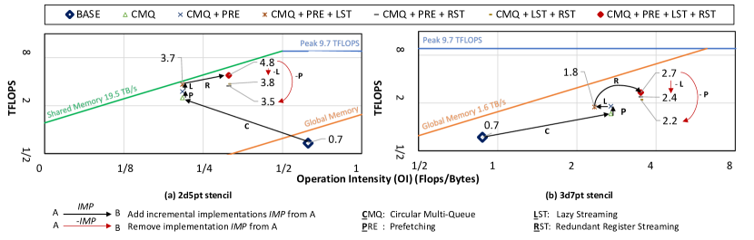
Figure 9. Roofline plots for different implementations in Section 4. We plot 2D 5-Point Jacobian stencil implementations to represent 2D stencils and 3D 7-Point Jacobian stencil implementations to represent 3D stencils. The black arrows link the incremental implementations from a $BASE$ implementations. The 3D $BASE$ applies device tiling (Section 4.1). The $LST$ refers to thread block level lazy streaming. Device tiling without lazy streaming will be extremely slow as can be inferred in Section 5.2.2.

7.4. Performance Breakdown

The remarkable speedup achieved by EBISU in comparison to other SOTA methods can be attributed to a fundamental shift in GPU programming principles. While existing SOTAs typically focus on constraining resources to enhance parallelism, EBISU constrains parallelism to optimize resource utilization. This novel approach enables the implementation of resource-scalable schemes, which ultimately contribute to EBISU’s performance.

In this section, we provide a detailed explanation of how the optimizations proposed in earlier sections impact the performance of EBISU. To demystify their effects, we present case studies involving 2D 5-Point Jacobian stencils (representing 2D stencils) and 3D 7-Point Jacobian stencils (representing 3D stencils). Figure 9 displays the roofline plot of various implementations, with the black arrow indicating the incremental implementation of each scheme.

For the roofline analysis, we report the performance as measured in TFLOPS (teraflops). Table 2 shows the relationship between TFLOPS and GCells/s metrics.

7.4.1. BASE

The BASE implementation refers to the approach that applies minimal parallelism analysis, as discussed in Section 6.1. In this phase, we prepare the necessary resources for EBISU. It is important to note that in the case of the 3D 7-Point stencil, the BASE implementation already incorporates device tiling, similar to the approach employed in the existing research of PERKS (Zhang et al., 2023).

7.4.2. Circular Multi-Queue (CMQ)

CMQ is a foundation for deep temporal blocking. As Figure 9 shows, in 2D stencils, we increase the depth of temporal blocking to move the bottleneck from global memory to shared memory. In 3D stencils, due to the shared memory’s limited capacity, we only move the Operation Intensity (OI) from left to right. Either way, we move the OI such that we increase the attainable performance shown in the roofline model.

7.4.3. Prefetching (PRE)

As Figure 9 shows, the PRE scheme has the effect of moving the roofline plot towards the attainable bound. However, it does not directly impact the attainable bound itself.

7.4.4. Lazy Streaming (LST)

The LST scheme aims to reduce synchronizations by using long buffers. By default, we employ LST to minimize device level synchronizations. This section specifically focuses on the impact of LST on reducing thread block synchronizations. As illustrated in Figure 9.a, applying LST to the 2D 5-point stencil brings its performance closer to the attainable bound. However, in the case of the 3D stencil, as shown in Figure 9.b, applying LST may harm performance. This is primarily due to the global memory still being the bottleneck, and the additional on-chip memory space required by LST implementation leads to a shallower temporal blocking. This results in a leftward shift in the OI, which consequently reduces the attainable performance. It is worth nothing that in the final version of EBISU, disabling LST for the 3D 7-point stencil allows for a doubling of the temporal blocking depth, from $t=8$ to $t=16$, leading to a performance increase from 2.7 TB/s to 2.9 TB/s. However, when excluding the redundant halo, the performance dips from 2.4 TB/s to 2.3 TB/s. Therefore, this result has been excluded from the discussion

7.4.5. Redundant Register Streaming (RST)

RST’s primary goal is to cut down shared memory access time (refer to Table 2). By doing so, we can shift the roofline plot closer to the compute bound from left to right when shared memory is the bottleneck (as shown in Figure 9.a). Also, we leverage RST to cache a portion of the tiling, which helps reduce the amount of data cached in shared memory. This enables us to achieve deeper temporal blocking and move the roofline plots closer to the compute bound from left to right, when global memory remains the bottleneck (as shown in Figure 9.b).

7.4.6. Relations Between Optimizations

The PRE and LST optimizations have the effect of improving performance and bringing it closer to the attainable bound. The RST optimization is designed to shift the roofline plots to the right, to increase the attainable bound. Red arrows in Figure 9 clearly shows that disabling either of these optimizations results in a degradation of performance.

7.4.7. Practical Attainable Performance

In 2D 5-point stencil, we achieved $4.8$ TFLOPS ($80\%$ of the attainable bound). In 3D 7-point stencil, we achieved $2.7$ TFLOPS ($50\%$ of the attainable bound). The big gap is due to the omission of the overheads in roofline model. As we consider overhead in our model (Section 5), we achieved $88\%$ and $80\%$ of $\mathbb{PP}$ in 2D 5-point and 3D 7-point stencils respectively. A model that considers the overheads can model the practical attainable performance better. As such, this model contributing to the decision-making also benefits the performance of EBISU.

8. Related works

Apart from the tiling optimizations we covered in Section 2.1, there are many stencil optimizations that are architecture-specific. For example, vectorization (Zhao et al., 2019; Yuan et al., 2021; Henretty et al., 2011); cache optimizations on CPUs (Wellein et al., 2009; Tang et al., 2015; Malas et al., 2015; Akbudak et al., 2020). For GPUs (Rawat et al., 2016; Grosser et al., 2014a; Holewinski et al., 2012), Chen et al. proposed an execution model on top of the shuffle operation on GPU (Chen et al., 2019); Liu et al. uses tensor cores to accelerate low precision stencils (Liu et al., 2022). Rawat et al. also summarized optimizations that can be used in stencil optimization, i.e., streaming, unrolling, prefetching (Rawat et al., 2019), and register reorder (Rawat et al., 2018a).

State-of-the-art implementations are usually built on top of multiple optimizations. For example, wavefront diamond blocking (Malas et al., 2015) is built on top of vectorization, cache optimization, streaming, and diamond tiling, STENCILGEN (Rawat et al., 2018b) is built on top of shared memory optimization, streaming, and N.5D tiling.

But combining different optimizations is tedious for implementation. Many researches focus on autocode generation using on domain specific language (Rawat et al., 2018b; Maruyama et al., 2011; Zhao et al., 2018), or compiler-based approaches (Verdoolaege et al., 2013; Ragan-Kelley et al., 2013). Some optimizations, especially those related to registers, are difficult to implement manually. Matsumura et al. implemented AN5D (Matsumura et al., 2020) that generates codes using registers effectively.

9. Conclusion and Future Work

In this paper we propose, EBISU, a novel temporal blocking approach. EBISU relies on low occupancy and mapping on large tiles over the device. The freed resources are then used to improve the data locality. We compared EBISU with two state-of-the-art temporal blocking implementations and two state-of-the-art autotuning tools. EBISU constantly shows its performance advantage. It achieves a geomean speedup of $1.49$x over any of the top alternative state-of-the-art implementations for each stencil benchmark.

This paper focuses on studying how modern GPU characteristics influence the optimization of temporal blocking stencils. Nevertheless, as EBISU proved effective, its optimization approach can be absorbed into production libraries like Halide (Ragan-Kelley et al., 2013) so that the end user can get the performance with minimal effort.

- (1)
- top (2023) 2023. TOP500. https://www.top500.org/lists/top500/2022/06/highs/ [Online; accessed 19-Jan-2023].
- Akbudak et al. (2020) Kadir Akbudak, Hatem Ltaief, Vincent Etienne, Rached Abdelkhalak, Thierry Tonellot, and David Keyes. 2020. Asynchronous computations for solving the acoustic wave propagation equation. The International Journal of High Performance Computing Applications 34, 4 (2020), 377–393.
- Berger and Oliger (1984) Marsha J Berger and Joseph Oliger. 1984. Adaptive mesh refinement for hyperbolic partial differential equations. Journal of computational Physics 53, 3 (1984), 484–512.
- Bondhugula et al. (2017) Uday Bondhugula, Vinayaka Bandishti, and Irshad Pananilath. 2017. Diamond Tiling: Tiling Techniques to Maximize Parallelism for Stencil Computations. IEEE Trans. Parallel Distrib. Syst. 28, 5 (May 2017), 1285–1298. https://doi.org/10.1109/TPDS.2016.2615094
- Chen et al. (2018) Peng Chen, Mohamed Wahib, Shinichiro Takizawa, Ryousei Takano, and Satoshi Matsuoka. 2018. Efficient Algorithms for the Summed Area Tables Primitive on GPUs. In 2018 IEEE International Conference on Cluster Computing (CLUSTER). 482–493. https://doi.org/10.1109/CLUSTER.2018.00064
- Chen et al. (2019) Peng Chen, Mohamed Wahib, Shinichiro Takizawa, Ryousei Takano, and Satoshi Matsuoka. 2019. A Versatile Software Systolic Execution Model for GPU Memory-Bound Kernels. In Proceedings of the International Conference for High Performance Computing, Networking, Storage and Analysis (Denver, Colorado) (SC ’19). Association for Computing Machinery, New York, NY, USA, Article 53, 81 pages. https://doi.org/10.1145/3295500.3356162
- CUDA (2022) Nvidia CUDA. 2022. CUDA C Programming Guide. https://docs.nvidia.com/cuda/cuda-c-programming-guide/ [Online; accessed 31-Dec-2022].
- Datta et al. (2009) Kaushik Datta, Shoaib Kamil, Samuel Williams, Leonid Oliker, John Shalf, and Katherine Yelick. 2009. Optimization and performance modeling of stencil computations on modern microprocessors. SIAM review 51, 1 (2009), 129–159.
- Datta et al. (2008) Kaushik Datta, Mark Murphy, Vasily Volkov, Samuel Williams, Jonathan Carter, Leonid Oliker, David Patterson, John Shalf, and Katherine Yelick. 2008. Stencil computation optimization and auto-tuning on state-of-the-art multicore architectures. In SC’08: Proceedings of the 2008 ACM/IEEE conference on Supercomputing. IEEE, 1–12.
- Endo (2018) Toshio Endo. 2018. Applying recursive temporal blocking for stencil computations to deeper memory hierarchy. In 2018 IEEE 7th Non-Volatile Memory Systems and Applications Symposium (NVMSA). IEEE, 19–24.
- Grosser et al. (2014a) Tobias Grosser, Albert Cohen, Justin Holewinski, Ponuswamy Sadayappan, and Sven Verdoolaege. 2014a. Hybrid hexagonal/classical tiling for GPUs. In Proceedings of Annual IEEE/ACM International Symposium on Code Generation and Optimization. 66–75.
- Grosser et al. (2013) Tobias Grosser, Albert Cohen, Paul H. J. Kelly, J. Ramanujam, P. Sadayappan, and Sven Verdoolaege. 2013. Split Tiling for GPUs: Automatic Parallelization Using Trapezoidal Tiles. In Proceedings of the 6th Workshop on General Purpose Processor Using Graphics Processing Units (Houston, Texas, USA) (GPGPU-6). Association for Computing Machinery, New York, NY, USA, 24–31. https://doi.org/10.1145/2458523.2458526
- Grosser et al. (2014b) Tobias Grosser, Sven Verdoolaege, Albert Cohen, and P. Sadayappan. 2014b. The Relation Between Diamond Tiling and Hexagonal Tiling. Parallel Processing Letters 24, 03 (2014), 1441002. https://doi.org/10.1142/S0129626414410023 arXiv:https://doi.org/10.1142/S0129626414410023
- Hagedorn et al. (2018) Bastian Hagedorn, Larisa Stoltzfus, Michel Steuwer, Sergei Gorlatch, and Christophe Dubach. 2018. High performance stencil code generation with lift. In Proceedings of the 2018 International Symposium on Code Generation and Optimization. 100–112.
- Henretty et al. (2011) Tom Henretty, Kevin Stock, Louis-Noël Pouchet, Franz Franchetti, J Ramanujam, and P Sadayappan. 2011. Data layout transformation for stencil computations on short-vector simd architectures. In International Conference on Compiler Construction. Springer, 225–245.
- Holewinski et al. (2012) Justin Holewinski, Louis-Noël Pouchet, and P. Sadayappan. 2012. High-performance Code Generation for Stencil Computations on GPU Architectures. In Proceedings of the 26th ACM International Conference on Supercomputing (San Servolo Island, Venice, Italy) (ICS ’12). ACM, New York, NY, USA, 311–320. https://doi.org/10.1145/2304576.2304619
- Irigoin and Triolet (1988) F. Irigoin and R. Triolet. 1988. Supernode Partitioning. In Proceedings of the 15th ACM SIGPLAN-SIGACT Symposium on Principles of Programming Languages (San Diego, California, USA) (POPL ’88). ACM, New York, NY, USA, 319–329. https://doi.org/10.1145/73560.73588
- Jiang (2023) Zhonghui Jiang. 2023. DRSTENCIL codebase. https://github.com/simple86/DRStencil [Online; accessed 22-Jan-2023].
- Kim et al. (2011) Ki-Hwan Kim, KyoungHo Kim, and Q-Han Park. 2011. Performance analysis and optimization of three-dimensional FDTD on GPU using roofline model. Computer Physics Communications 182, 6 (2011), 1201–1207.
- Liu et al. (2022) Xiaoyan Liu, Yi Liu, Hailong Yang, Jianjin Liao, Mingzhen Li, Zhongzhi Luan, and Depei Qian. 2022. Toward accelerated stencil computation by adapting tensor core unit on GPU. In Proceedings of the 36th ACM International Conference on Supercomputing. 1–12.
- Malas et al. (2015) Tareq Malas, Georg Hager, Hatem Ltaief, Holger Stengel, Gerhard Wellein, and David Keyes. 2015. Multicore-optimized wavefront diamond blocking for optimizing stencil updates. SIAM Journal on Scientific Computing 37, 4 (2015), C439–C464.
- Maruyama and Aoki (2014) Naoya Maruyama and Takayuki Aoki. 2014. Optimizing Stencil Computations for NVIDIA Kepler GPUs. In Proceedings of the 1st International Workshop on High-Performance Stencil Computations, Armin Größlinger and Harald Köstler (Eds.). Vienna, Austria, 89–95.
- Maruyama et al. (2011) Naoya Maruyama, Tatsuo Nomura, Kento Sato, and Satoshi Matsuoka. 2011. Physis: an implicitly parallel programming model for stencil computations on large-scale GPU-accelerated supercomputers. In Proceedings of 2011 International Conference for High Performance Computing, Networking, Storage and Analysis. 1–12.
- Matsumura (2023) Kazuaki Matsumura. 2023. AN5D AD/AE. https://github.com/khaki3/AN5D-Artifact [Online; accessed 22-Jan-2023].
- Matsumura et al. (2020) Kazuaki Matsumura, Hamid Reza Zohouri, Mohamed Wahib, Toshio Endo, and Satoshi Matsuoka. 2020. AN5D: automated stencil framework for high-degree temporal blocking on GPUs. In CGO ’20: 18th ACM/IEEE International Symposium on Code Generation and Optimization, San Diego, CA, USA, February, 2020. 199–211. https://doi.org/10.1145/3368826.3377904
- Mei and Chu (2016) Xinxin Mei and Xiaowen Chu. 2016. Dissecting GPU memory hierarchy through microbenchmarking. IEEE Transactions on Parallel and Distributed Systems 28, 1 (2016), 72–86.
- Meng and Skadron (2009) Jiayuan Meng and Kevin Skadron. 2009. Performance Modeling and Automatic Ghost Zone Optimization for Iterative Stencil Loops on GPUs. In Proceedings of the 23rd International Conference on Supercomputing (Yorktown Heights, NY, USA) (ICS ’09). ACM, New York, NY, USA, 256–265. https://doi.org/10.1145/1542275.1542313
- Muranushi and Makino (2015) Takayuki Muranushi and Junichiro Makino. 2015. Optimal Temporal Blocking for Stencil Computation. Procedia Computer Science 51 (2015), 1303–1312. https://doi.org/10.1016/j.procs.2015.05.315 International Conference On Computational Science, ICCS 2015.
- Nguyen et al. (2010) Anthony Nguyen, Nadathur Satish, Jatin Chhugani, Changkyu Kim, and Pradeep Dubey. 2010. 3.5-D blocking optimization for stencil computations on modern CPUs and GPUs. In SC’10: Proceedings of the 2010 ACM/IEEE International Conference for High Performance Computing, Networking, Storage and Analysis. IEEE, 1–13.
- Nvidia (2022a) Nvidia. 2022a. Inside Kepler. https://www.nvidia.com/content/dam/en-zz/Solutions/Data-Center/tesla-product-literature/NVIDIA-Kepler-GK110-GK210-Architecture-Whitepaper.pdf
- Nvidia (2022b) Nvidia. 2022b. NVIDIA A100 Tensor Core GPU Architecture. https://www.nvidia.com/content/dam/en-zz/Solutions/Data-Center/nvidia-ampere-architecture-whitepaper.pdf
- Ofenbeck et al. (2014) Georg Ofenbeck, Ruedi Steinmann, Victoria Caparros, Daniele G Spampinato, and Markus Püschel. 2014. Applying the roofline model. In 2014 IEEE International Symposium on Performance Analysis of Systems and Software (ISPASS). IEEE, 76–85.
- Podobas et al. (2020) Artur Podobas, Kentaro Sano, and Satoshi Matsuoka. 2020. A template-based framework for exploring coarse-grained reconfigurable architectures. In 2020 IEEE 31st International Conference on Application-specific Systems, Architectures and Processors (ASAP). IEEE, 1–8.
- Ragan-Kelley et al. (2013) Jonathan Ragan-Kelley, Connelly Barnes, Andrew Adams, Sylvain Paris, Frédo Durand, and Saman Amarasinghe. 2013. Halide: A Language and Compiler for Optimizing Parallelism, Locality, and Recomputation in Image Processing Pipelines. In Proceedings of the 34th ACM SIGPLAN Conference on Programming Language Design and Implementation (Seattle, Washington, USA) (PLDI ’13). Association for Computing Machinery, New York, NY, USA, 519–530. https://doi.org/10.1145/2491956.2462176
- Rawat et al. (2015) Prashant Rawat, Martin Kong, Tom Henretty, Justin Holewinski, Kevin Stock, Louis-Noël Pouchet, J. Ramanujam, Atanas Rountev, and P. Sadayappan. 2015. SDSLc: A Multi-Target Domain-Specific Compiler for Stencil Computations. In Proceedings of the 5th International Workshop on Domain-Specific Languages and High-Level Frameworks for High Performance Computing (Austin, Texas) (WOLFHPC ’15). Association for Computing Machinery, New York, NY, USA, Article 6, 10 pages. https://doi.org/10.1145/2830018.2830025
- Rawat (2023a) Prashant Singh Rawat. 2023a. ARTEMIS codebase. https://github.com/pssrawat/artemis [Online; accessed 22-Jan-2023].
- Rawat (2023b) Prashant Singh Rawat. 2023b. STENCILGEN AD/AE. https://github.com/pssrawat/IEEE2017 [Online; accessed 22-Jan-2023].
- Rawat et al. (2016) Prashant Singh Rawat, Changwan Hong, Mahesh Ravishankar, Vinod Grover, Louis-Noël Pouchet, and P Sadayappan. 2016. Effective resource management for enhancing performance of 2D and 3D stencils on GPUs. In Proceedings of the 9th Annual Workshop on General Purpose Processing using Graphics Processing Unit. 92–102.
- Rawat et al. (2018a) Prashant Singh Rawat, Fabrice Rastello, Aravind Sukumaran-Rajam, Louis-Noël Pouchet, Atanas Rountev, and P. Sadayappan. 2018a. Register Optimizations for Stencils on GPUs. SIGPLAN Not. 53, 1 (Feb. 2018), 168–182. https://doi.org/10.1145/3200691.3178500
- Rawat et al. (2018b) Prashant Singh Rawat, Miheer Vaidya, Aravind Sukumaran-Rajam, Mahesh Ravishankar, Vinod Grover, Atanas Rountev, Louis-Noël Pouchet, and P Sadayappan. 2018b. Domain-specific optimization and generation of high-performance GPU code for stencil computations. Proc. IEEE 106, 11 (2018), 1902–1920.
- Rawat et al. (2019) Prashant Singh Rawat, Miheer Vaidya, Aravind Sukumaran-Rajam, Atanas Rountev, Louis-Noël Pouchet, and P Sadayappan. 2019. On optimizing complex stencils on GPUs. In 2019 IEEE International Parallel and Distributed Processing Symposium (IPDPS). IEEE, 641–652.
- Shende and Malony (2006) Sameer S Shende and Allen D Malony. 2006. The TAU parallel performance system. The International Journal of High Performance Computing Applications 20, 2 (2006), 287–311.
- Stengel et al. (2015) Holger Stengel, Jan Treibig, Georg Hager, and Gerhard Wellein. 2015. Quantifying performance bottlenecks of stencil computations using the execution-cache-memory model. In Proceedings of the 29th ACM on International Conference on Supercomputing. 207–216.
- Svedin et al. (2021) Martin Svedin, Steven WD Chien, Gibson Chikafa, Niclas Jansson, and Artur Podobas. 2021. Benchmarking the nvidia gpu lineage: From early k80 to modern a100 with asynchronous memory transfers. In Proceedings of the 11th International Symposium on Highly Efficient Accelerators and Reconfigurable Technologies. 1–6.
- Tang et al. (2015) Yuan Tang, Ronghui You, Haibin Kan, Jesmin Jahan Tithi, Pramod Ganapathi, and Rezaul A Chowdhury. 2015. Cache-oblivious wavefront: improving parallelism of recursive dynamic programming algorithms without losing cache-efficiency. In Proceedings of the 20th ACM SIGPLAN Symposium on Principles and Practice of Parallel Programming. 205–214.
- van Werkhoven (2019) Ben van Werkhoven. 2019. Kernel Tuner: A search-optimizing GPU code auto-tuner. Future Generation Computer Systems 90 (2019), 347–358. https://doi.org/10.1016/j.future.2018.08.004
- Verdoolaege et al. (2013) Sven Verdoolaege, Juan Carlos Juega, Albert Cohen, Jose Ignacio Gomez, Christian Tenllado, and Francky Catthoor. 2013. Polyhedral parallel code generation for CUDA. ACM Transactions on Architecture and Code Optimization (TACO) 9, 4 (2013), 1–23.
- Volkov (2010) Vasily Volkov. 2010. Better performance at lower occupancy. In Proceedings of the GPU technology conference, GTC, Vol. 10. San Jose, CA, 16.
- Wahib and Maruyama (2015) Mohamed Wahib and Naoya Maruyama. 2015. Automated GPU Kernel Transformations in Large-Scale Production Stencil Applications. In Proceedings of the 24th International Symposium on High-Performance Parallel and Distributed Computing (Portland, Oregon, USA) (HPDC ’15). Association for Computing Machinery, New York, NY, USA, 259–270. https://doi.org/10.1145/2749246.2749255
- Waidyasooriya et al. (2016) Hasitha Muthumala Waidyasooriya, Yasuhiro Takei, Shunsuke Tatsumi, and Masanori Hariyama. 2016. OpenCL-based FPGA-platform for stencil computation and its optimization methodology. IEEE Transactions on Parallel and Distributed Systems 28, 5 (2016), 1390–1402.
- Wellein et al. (2009) Gerhard Wellein, Georg Hager, Thomas Zeiser, Markus Wittmann, and Holger Fehske. 2009. Efficient temporal blocking for stencil computations by multicore-aware wavefront parallelization. In 2009 33rd Annual IEEE International Computer Software and Applications Conference, Vol. 1. IEEE, 579–586.
- Wolfe (1989) M. Wolfe. 1989. More Iteration Space Tiling. In Proceedings of the 1989 ACM/IEEE Conference on Supercomputing (Reno, Nevada, USA) (Supercomputing ’89). ACM, New York, NY, USA, 655–664. https://doi.org/10.1145/76263.76337
- Wong et al. (2010) Henry Wong, Misel-Myrto Papadopoulou, Maryam Sadooghi-Alvandi, and Andreas Moshovos. 2010. Demystifying GPU microarchitecture through microbenchmarking. In 2010 IEEE International Symposium on Performance Analysis of Systems & Software (ISPASS). 235–246. https://doi.org/10.1109/ISPASS.2010.5452013
- You et al. (2021) X. You, H. Yang, Z. Jiang, Z. Luan, and D. Qian. 2021. DRStencil: Exploiting Data Reuse within Low-order Stencil on GPU. In 2021 IEEE 23rd Int Conf on High Performance Computing & Communications; 7th Int Conf on Data Science & Systems; 19th Int Conf on Smart City; 7th Int Conf on Dependability in Sensor, Cloud & Big Data Systems & Application (HPCC/DSS/SmartCity/DependSys). IEEE Computer Society, Los Alamitos, CA, USA, 63–70. https://doi.org/10.1109/HPCC-DSS-SmartCity-DependSys53884.2021.00036
- Yuan et al. (2021) Liang Yuan, Hang Cao, Yunquan Zhang, Kun Li, Pengqi Lu, and Yue Yue. 2021. Temporal Vectorization for Stencils. In Proceedings of the International Conference for High Performance Computing, Networking, Storage and Analysis (St. Louis, Missouri) (SC ’21). Association for Computing Machinery, New York, NY, USA, Article 82, 13 pages. https://doi.org/10.1145/3458817.3476149
- Zhang et al. (2023) Lingqi Zhang, Mohamed Wahib, Peng Chen, Jintao Meng, Xiao Wang, Toshio Endo, and Satoshi Matsuoka. 2023. PERKS: a Locality-Optimized Execution Model for Iterative Memory-bound GPU Applications. arXiv preprint arXiv:2204.02064 (2023).
- Zhang et al. (2020) Lingqi Zhang, Mohamed Wahib, Haoyu Zhang, and Satoshi Matsuoka. 2020. A Study of Single and Multi-device Synchronization Methods in Nvidia GPUs. In 2020 IEEE International Parallel and Distributed Processing Symposium (IPDPS). 483–493. https://doi.org/10.1109/IPDPS47924.2020.00057
- Zhao et al. (2019) Tuowen Zhao, Protonu Basu, Samuel Williams, Mary Hall, and Hans Johansen. 2019. Exploiting reuse and vectorization in blocked stencil computations on CPUs and GPUs. In Proceedings of the International Conference for High Performance Computing, Networking, Storage and Analysis. 1–44.
- Zhao et al. (2018) Tuowen Zhao, Samuel Williams, Mary Hall, and Hans Johansen. 2018. Delivering Performance-Portable Stencil Computations on CPUs and GPUs Using Bricks. In 2018 IEEE/ACM International Workshop on Performance, Portability and Productivity in HPC (P3HPC). 59–70. https://doi.org/10.1109/P3HPC.2018.00009
- Zohouri et al. (2018) Hamid Reza Zohouri, Artur Podobas, and Satoshi Matsuoka. 2018. Combined Spatial and Temporal Blocking for High-Performance Stencil Computation on FPGAs Using OpenCL. In Proceedings of the 2018 ACM/SIGDA International Symposium on Field-Programmable Gate Arrays (Monterey, CALIFORNIA, USA) (FPGA ’18). Association for Computing Machinery, New York, NY, USA, 153–162. https://doi.org/10.1145/3174243.3174248