Bayesian Estimation of Laser Linewidth from Delayed Self-Heterodyne Measurements

Abstract

We present a statistical inference approach to estimate the frequency noise characteristics of ultra-narrow linewidth lasers from delayed self-heterodyne beat note measurements using Bayesian inference. Particular emphasis is on estimation of the intrinsic (Lorentzian) laser linewidth. The approach is based on a statistical model of the measurement process, taking into account the effects of the interferometer as well as the detector noise. Our method therefore yields accurate results even when the intrinsic linewidth plateau is obscured by detector noise. The regression is performed on periodogram data in the frequency domain using a Markov-chain Monte Carlo method. By using explicit knowledge about the statistical distribution of the observed data, the method yields good results already from a single time series and does not rely on averaging over many realizations, since the information in the available data is evaluated very thoroughly. The approach is demonstrated for simulated time series data from a stochastic laser rate equation model with $1/f$–type non-Markovian noise.

1 Introduction

Ultra-narrow linewidth lasers are critical components of many applications in modern science and technology, ranging from precision metrology, e.g., gravitational wave interferometers Abbott2009 and optical atomic clocks Ludlow2015 , to coherent optical communication systems Kikuchi2016 and ion-trap quantum computers Akerman2015 . To perform well in these technologies, the laser requires a high degree of spectral coherence, i.e., a well-defined phase, and/ or a sharply defined frequency and thus low frequency noise. The (intrinsic) laser linewidth is quantified by the width of the optical power spectrum, which in real systems is usually broadened by additional $1/f$–like technical noise (also flicker noise) Kikuchi1989 ; Mercer1991 ; Stephan2005 . As the width of the optical power spectrum is dominantly determined by the frequency noise, the corresponding frequency noise power spectral density (FN–PSD) provides an almost complete characterization of the spectral quality of the laser, where the effects of non-Markovian noise can be well separated from that of white noise. The latter manifests itself as a plateau in the high-frequency part of the FN–PSD, from which the intrinsic (Lorentzian) laser linewidth Henry1986 ; Wenzel2021 can be deduced, that is of major interest for most of the aforementioned applications. In ultra-narrow linewidth lasers, the determination of the white noise plateau can be challenging, since it often sets in only at very high frequencies and is obscured by $1/f$–type noise (at low frequencies) or by detector noise (at high frequencies).

The standard technique for the experimental measurement of the laser linewidth is the delayed self-heterodyne (DSH) method Okoshi1980 ; Schiemangk2014 , which involves measuring the beat signal between the optical field with a delayed and frequency-shifted copy of itself. This method is attractive because it can provide a direct measurement of the linewidth without the need for an external frequency standard or active frequency stabilization. Evaluation of the DSH measurement data is however non-trivial, as both the footprint of the interferometer as well as the detector noise must be removed in order to obtain an artifact-free reconstruction of the FN–PSD Kantner2023 .

In this paper, we present a Bayesian estimation approach to infer on the laser’s FN–PSD from time series data. Our method is based on statistical modeling of the DSH measurement process and allows to extract accurate estimates of key parameters such as the intrinsic linewidth, even when the white noise plateau is obscured by detector noise. The method is demonstrated for simulated time series data based on a stochastic rate equation model for a single-mode semiconductor laser.

2 Delayed Self-Heterodyne Method

2.1 Experimental Setup

The DSH method is a standard technique for measuring the laser linewidth Schiemangk2014 , particularly of ultra-narrow linewidth lasers. It involves splitting of the laser beam into two paths using an acousto-optic modulator (AOM), where one of the two beams is also frequency-shifted, see Fig. 1. The frequency-shifted beam is then delayed using a long fiber before being finally superimposed with the other beam at a photodetector. The optical field received by the detector $E\left(t\right)=\mathrm{Re}\left(\mathcal{E}\left(t\right)\right)$ reads

$$\mathcal{E}\left(t\right)=\sqrt{P\left(t\right)}\,\mathrm{e}^{i\left(\omega_{0}t+\phi\left(t\right)\right)}+\sqrt{P\left(t-\tau_{d}\right)}\,\mathrm{e}^{i\left(\left(\omega_{0}+\Delta\omega\right)\left(t-\tau_{d}\right)+\phi\left(t-\tau_{d}\right)\right)}+\xi_{E}\left(t\right),$$ (1)

where $\omega_{0}$ is the nominal continuous wave (CW) frequency, $\tau_{d}$ is the interferometer delay, $\phi\left(t\right)$ is the (randomly fluctuating) optical phase, $P\left(t\right)$ is the (fluctuating) amplitude and $\Delta\omega$ is the frequency shift induced by the AOM. Moreover, $\xi_{E}\left(t\right)$ describes additive detector noise. Conventional photodetectors capture only the slow beat note in the intensity signal $I\left(t\right)\propto\left|E\left(t\right)\right|^{2}$. The spectrum analyzer then further downshifts the beat frequency and removes the DC component of the signal. From this signal and its quadrature component (generated by a Hilbert transform), one can then extract the phase jitter and finally conclude on the fluctuations of the instantaneous laser frequency Kantner2023 .

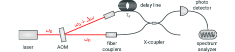
Figure 1: Experimental setup of the DSH method, where an acousto-optic modulator (AOM) separates the incoming laser beam into two beams. One part of the signal is delayed by a long fiber and frequency shifted. The two beams are superimposed at a photodetector, which captures only the slow beat note signal. The picture is reprinted with permission from Ref. Kantner2023 .

2.2 Periodogram and Power Spectral Density

The power spectral density (PSD) $S_{z,z}\left(\omega\right)$ of a stationary stochastic process $z\left(t\right)$ is given by the Fourier transform of its auto-correlation function $C_{z,z}\left(\tau\right)=\langle z\left(t\right)z\left(t+\tau\right)\rangle$ (Wiener–Khinchin theorem). Given only a sample of the trajectory (in discrete time), the PSD is typically estimated from the periodogram Priestley1982 ; Madsen2007 , which is given by the absolute square of the (discrete) Fourier transform of the time series

$$\widehat{S}_{z,z}\left(\omega\right)=\left|\mathcal{F}\left[z\left(t\right)\right]\left(\omega\right)\right|^{2}.$$ (2)

The PSD then follows as the expectation value of the periodogram (ensemble mean)

$$S_{z,z}\left(\omega\right)=\langle\widehat{S}_{z,z}\left(\omega\right)\rangle.$$ (3)

Our goal is to estimate the FN–PSD of the free-running laser, which will be denoted by $S_{x,x}\left(\omega\right)$ in the following. As the frequency follows from the optical phase by differentiation with respect to time $\omega\left(t\right)=\dot{\phi}\left(t\right)$, their PSDs are connected by

$$S_{x,x}\left(\omega\right)=\omega^{2}S_{\phi,\phi}\left(\omega\right).$$ (4)

Note that the FN–PSD $S_{x,x}\left(\omega\right)$ is not directly observed in the experiment, but must be reconstructed from the phase jitter $\phi\left(t\right)-\phi\left(t-\tau_{d}\right)$, that can be deduced from the slow beat note of the intensity time series corresponding to Eq. (1).

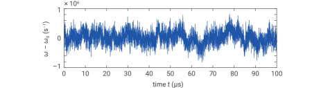
Figure 2: Simulated time series of frequency fluctuations $\omega\left(t\right)=\dot{\phi}\left(t\right)$ around the nominal continuous wave frequency $\omega_{0}$. The instantaneous laser frequency exhibits characteristic drifts, which are commonly observed in semiconductor lasers. The time series has been simulated using the SDE model (14), where frequency drifts are induced by the $1/f$–type colored noise contributions. The trajectory in the plot shows a moving average (over 50 ns) to improve the visibility of the effect.

In the following, we describe the measured signal of the DSH experiment (in terms of frequency fluctuations) by

$$z\left(t\right)=\left(h*x\right)\left(t\right)+\xi\left(t\right),$$ (5)

where $z\left(t\right)$ is the observed time series, the convolution kernel $h\left(t\right)=\delta\left(t\right)-\delta\left(t-\tau_{d}\right)$ is the transfer function of the interferometer, $x\left(t\right)$ is the hidden time series of the instantaneous frequency fluctuations of the laser (i.e., $x\left(t\right)\;\hat{=}\;\omega\left(t\right)-\omega_{0}=\dot{\phi}\left(t\right)$) and $\xi\left(t\right)$ is (colored) additive measurement noise (not correlated with the hidden signal). A sample time series of frequency fluctuations $x\left(t\right)$, which exhibits characteristic frequency drifts as commonly observed in semiconductor lasers, is shown in Fig. 2. Our goal is to characterize the statistical properties of the fluctuating time series $x\left(t\right)$. Fourier transform of Eq. (5) yields a relation between the PSDs of the observed and the hidden signal

$$S_{z,z}\left(\omega\right)=\left|H\left(\omega\right)\right|^{2}S_{x,x}\left(\omega\right)+S_{\xi,\xi}\left(\omega\right),$$ (6)

where the Fourier transformed transfer function reads

$$H\left(\omega\right)=1-\exp{\left(i\omega\tau_{d}\right)}.$$ (7)

The PSDs of the hidden signal and the detector noise are assumed to obey the following functional forms Kantner2023

$$S_{x,x}\left(\omega\right) =\frac{C}{\left|\omega\right|^{\nu}}+S_{\infty}, S_{\xi,\xi}\left(\omega\right) =\sigma^{2}\omega^{2}.$$ (8)

The model equation for $S_{x,x}\left(\omega\right)$ is a phenomenological relation Kikuchi1989 ; Mercer1991 that includes both $1/f^{\nu}$–type noise (described by $C$ and $\nu$) and a white noise plateau, where $S_{\infty}$ quantifies the intrinsic linewidth. The detector noise PSD $S_{\xi,\xi}\left(\omega\right)$ follows from the assumption of spectrally white phase fluctuation measurement noise, which must be multiplied by $\omega^{2}$ to arrive at the corresponding measurement noise for the frequency fluctuations, cf. Eq. (4). Figure 3 shows a double-logarithmic plot the PSDs considered here.

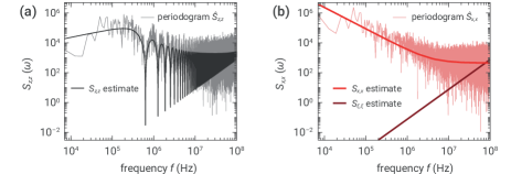
Figure 3: (a) Periodogram $\widehat{S}_{z,z}\left(\omega\right)$ of an observed time series $z\left(t\right)$ along with the power spectral density $S_{z,z}\left(\omega\right)$ estimated using the MCMC method. The signal features sharp dropouts at the roots of the transfer function (7) at frequencies $f_{n}=n/\tau_{d}$, $n\in\mathbb{Z}$. (b) Estimated FN–PSD $S_{x,x}\left(\omega\right)$ and periodogram $\widehat{S}_{x,x}\left(\omega\right)$ of the hidden time series $x\left(t\right)$. The detector noise PSD $S_{\xi,\xi}\left(\omega\right)$ has a quadratic frequency dependency. Both PSDs are obtained from statistical inference on the observed periodogram $\widehat{S}_{z,z}\left(\omega\right)$.

3 Parameter Inference

For estimation of the parameters characterizing the FN–PSD of the laser, we perform a Bayesian regression on the PSD $S_{z,z}\left(\omega\right)$ of the detected signal using the transfer function (7) and the model relations (8), which have a highly nonlinear frequency dependency. In the regression procedure, we regard the periodogram $\widehat{S}_{z,z}(\omega)$ (available at a set of discrete frequencies) as observed data. In order to conduct a maximum likelihood estimation using frequency domain data, knowledge about the expected statistical distribution of the periodogram $\widehat{S}_{z,z}(\omega)$ is required.

The frequency fluctuations $x\left(t\right)$ and the measurement noise $\xi\left(t\right)$ are assumed to normally distributed, which is in excellent agreement with experimental data. The detected time series $z\left(t\right)$ observed at discrete instances of time is thus a multi-variate Gaussian characterized by its covariance matrix. By random variable transformation Priestley1982 we then find the periodogram of the measured time series to be exponentially distributed

$$\widehat{S}_{z,z}\left(\omega\right)\sim\mathrm{Exp}\left(\lambda\left(\omega,\boldsymbol{\theta}\right)\right),$$ (9)

where the probability distribution function (PDF)

$$p\left(\widehat{S}_{z,z}\left(\omega\right),\lambda\left(\omega,\boldsymbol{\theta}\right)\right)=\lambda\left(\omega,\boldsymbol{\theta}\right)\mathrm{e}^{-\lambda\left(\omega,\boldsymbol{\theta}\right)\,\widehat{S}_{z,z}\left(\omega\right)},$$ (10)

is characterized by a parameter $\lambda$ that depends on frequency $\omega$ and the unknown parameters $\boldsymbol{\theta}=\left(C,\nu,S_{\infty},\sigma\right)^{T}$. We identify the parameter function $\lambda\left(\omega,\boldsymbol{\theta}\right)$ with the inverse expectation value of the periodogram data given by Eq. (6) such that

$$\frac{1}{\lambda\left(\omega,\boldsymbol{\theta}\right)}=S_{z,z}\left(\omega,\boldsymbol{\theta}\right)=\left|H\left(\omega\right)\right|^{2}S_{x,x}\left(\omega,\boldsymbol{\theta}\right)+S_{\xi,\xi}\left(\omega,\boldsymbol{\theta}\right).$$ (11)

The likelihood of observing a certain realization of the periodogram $\widehat{S}_{z,z}\left(\omega_{k}\right)$ (at a discrete set of frequencies $\omega_{k}$) given a set of parameters $\boldsymbol{\theta}$ is then given by the likelihood function

$$L\left(\boldsymbol{\theta}\right)=\prod_{k}p\left(\widehat{S}_{z,z}\left(\omega_{k}\right),\lambda\left(\omega_{k},\boldsymbol{\theta}\right)\right),$$ (12)

where the function $p$ is given by Eq. (10). Note that the underlying joint probability distribution factorizes here completely, as the periodogram data $\widehat{S}_{z,z}\left(\omega\right)$ at different frequencies are statistically independent.

Bayesian regression on the parameters $\boldsymbol{\theta}$ is now performed by maximizing the likelihood function (12) using a Markov chain Monte Carlo (MCMC) approach Naesseth2019 . We employ the Metropolis–Hastings algorithm to sample a Markov chain of parameter sets $\boldsymbol{\theta}^{\left(j-1\right)}\to\boldsymbol{\theta}^{\left(j\right)}\to\ldots$ that is distributed according to $L\left(\boldsymbol{\theta}\right)$. The maximum of this distribution is then located at the parameter set $\boldsymbol{\theta}^{\ast}$ which is most likely to underlie the observed data.

We would like to stress that in the present scenario the regression on spectral data (i.e., on the periodogram $\widehat{S}_{z,z}\left(\omega\right)$) as described above is advantageous compared to the direct estimation on time domain data. The reason for this is that the construction of the likelihood function for the observed time series is either conceptually challenging due to the long interferometer delay or would require a high-dimensional Markovian embedding. Furthermore, the system exhibits long-range time correlations due to the presence of $1/f$–type noise, which would require very long time series to be considered in the regression. These issues render the estimation procedure in the time domain computationally expensive, but can be easily overcome by transforming the problem into the frequency domain.

4 Results

We demonstrate the estimation method described above for simulated data using the stochastic laser rate equations given in Appendix A. The DSH measurement is simulated as described in Ref. Kantner2023 with simulation code that is available online Kantner2023b .

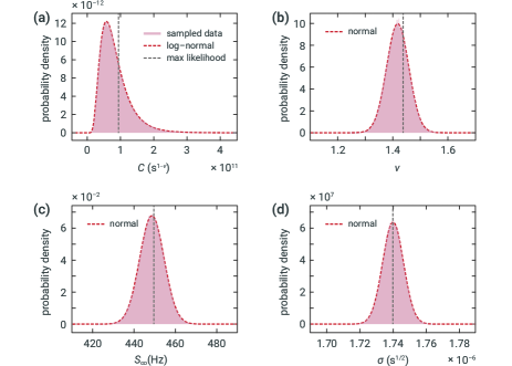
Figure 4: Histograms of estimated parameters characterizing the FN–PSD obtained using the MCMC method. The sampled distributions are shown along with normally (Gaussian) and log-normally distributed probability density distributions. The dashed black line indicates the position of the maximum likelihood estimate. The estimation results are summarized in Tab. 1.

Figure 4 shows histograms of the sampled Markov chains $\boldsymbol{\theta}^{\left(j\right)}$, which are estimators of the marginal distributions of the joint PDF of the parameters that is proportional to $L\left(\boldsymbol{\theta}\right)$. A notable feature of the MCMC method is that it provides not only an estimate of the most probable set of parameters but rather their entire distribution, allowing to asses the uncertainty of the estimates, see Tab. 1. In addition to the histogram, the plot also indicates the position of the maximum of $L\left(\boldsymbol{\theta}\right)$ as a dashed line. The corresponding parameter set $\boldsymbol{\theta}^{*}$ is denoted as the maximum likelihood estimator (MLE), i.e., the maximum of the joint PDF. It should be noted that these values partially differ significantly from the means of the marginal distributions. The reason for this is that the different parameters are strongly correlated, and the marginal distribution of $C$ has a maximum far from its mean. The mutual correlation of all parameter estimates is quantified by the matrix of Pearson correlation coefficients

$$\rho_{i,j}=\frac{\mathrm{Cov}\left(\theta_{i},\theta_{j}\right)}{\sqrt{\mathrm{Var}\left(\theta_{i}\right)\,\mathrm{Var}\left(\theta_{j}\right)}},$$ (13)

which is obtained as

$$\rho=\quad\hbox{}\vbox{\kern 0.86108pt\hbox{$\kern 0.0pt\kern 2.5pt\kern-5.0pt\left(\kern 0.0pt\kern-2.5pt\kern-6.66669pt\vbox{\kern-0.86108pt\vbox{\vbox{ \halign{\kern\arraycolsep\hfil\@arstrut$\kbcolstyle#$\hfil\kern\arraycolsep& \kern\arraycolsep\hfil$\@kbrowstyle#$\ifkbalignright\relax\else\hfil\fi\kern\arraycolsep&& \kern\arraycolsep\hfil$\@kbrowstyle#$\ifkbalignright\relax\else\hfil\fi\kern\arraycolsep\cr 5.0pt\hfil\@arstrut$\scriptstyle$\hfil\kern 5.0pt&5.0pt\hfil$\scriptstyle C$\hfil\kern 5.0pt&5.0pt\hfil$\scriptstyle\nu$\hfil\kern 5.0pt&5.0pt\hfil$\scriptstyle S_{\infty}$\hfil\kern 5.0pt&5.0pt\hfil$\scriptstyle\sigma\\C$\hfil\kern 5.0pt&5.0pt\hfil$\scriptstyle 1$\hfil\kern 5.0pt&5.0pt\hfil$\scriptstyle 0.93$\hfil\kern 5.0pt&5.0pt\hfil$\scriptstyle 0.41$\hfil\kern 5.0pt&5.0pt\hfil$\scriptstyle-0.14\\\nu$\hfil\kern 5.0pt&5.0pt\hfil$\scriptstyle$\hfil\kern 5.0pt&5.0pt\hfil$\scriptstyle 1$\hfil\kern 5.0pt&5.0pt\hfil$\scriptstyle 0.47$\hfil\kern 5.0pt&5.0pt\hfil$\scriptstyle-0.16\\S_{\infty}$\hfil\kern 5.0pt&5.0pt\hfil$\scriptstyle$\hfil\kern 5.0pt&5.0pt\hfil$\scriptstyle$\hfil\kern 5.0pt&5.0pt\hfil$\scriptstyle 1$\hfil\kern 5.0pt&5.0pt\hfil$\scriptstyle-0.46\\\sigma$\hfil\kern 5.0pt&5.0pt\hfil$\scriptstyle$\hfil\kern 5.0pt&5.0pt\hfil$\scriptstyle$\hfil\kern 5.0pt&5.0pt\hfil$\scriptstyle$\hfil\kern 5.0pt&5.0pt\hfil$\scriptstyle 1$\hfil\kern 5.0pt\crcr}}}}\right)$}}.$$

Indeed, one observes in Fig. 4 (b)–(d) that the MLE and the means of the marginal distributions differ more significantly, the stronger the respective parameter estimate is correlated with $C$. Moreover, we observe that the estimates of all parameters entering the signal PSD $S_{x,x}\left(\omega\right)$ are negatively correlated with the estimate of the detector noise parameter $\sigma$, which is expected from Eq. (6).

The MCMC routine was run with normally distributed proposal functions for the parameters $\nu$, $S_{\infty}$ and $\sigma$ and with a log-normal proposal distribution for $C$. The latter automatically enforces $C>0$ and provides an efficient sampling as it matches the shape of the target distribution. With the variances of the proposal distribution tuned appropriately, we achieved an acceptance rate of the proposed parameter samples of around $30\%$.

parameter (unit)	mean $\mathbf{\pm}$ std	MLE
$C\,(\mathrm{s}^{1-\nu})$	$\left(8.6\pm 4.8\right)\cdot 10^{10}$	$9.6\cdot 10^{10}$
$\nu$	$1.42\pm 0.04$	$1.44$
$S_{\infty}\,(\mathrm{Hz})$	$448.8\pm 5.9$	$449.6$
$\sigma\,(\mathrm{s}^{1/2})$	$1.74\cdot 10^{-6}\pm 6.4\cdot 10^{-9}$	$1.74\cdot 10^{-6}$

Table 1: Mean values and standard deviations (std) of the marginal distributions and the maximum likelihood estimator (MLE) of the parameters $\boldsymbol{\theta}$ obtained using the MCMC method.

5 Conclusions

The application of Bayesian inference methods to data from DSH laser linewidth measurements allows for an accurate extraction of the parameters characterizing the FN–PSD along with its uncertainties. Based on statistical modeling of the underlying measurement process, the method enables a reliable characterization of the spectral coherence of the laser even when the intrinsic linewidth plateau is obscured by detector noise. Furthermore, by invoking explicit assumptions about the statistical distribution of the measured data, the method extracts the information encoded in the available data very extensively, so that no averaging over many realizations or long times is required.

Appendix

A Stochastic Laser Rate Equations

We describe a set of Itô-type stochastic differential equations (SDEs) modeling the fluctuation dynamics of a generic single-mode semiconductor laser. In the presence of noise, the evolution of the photon number $P$, the optical phase $\phi$ and the carrier number $N$ in the active region is described by:

$$\mathrm{d}P =\left(-\gamma\left(P-P_{\mathrm{th}}\right)+\Gamma v_{g}g\left(P,N\right)P+\Gamma v_{g}g_{\mathrm{sp}}\left(P,N\right)+\sigma_{P}\left(P\right)\mathcal{F}_{P}\left(t\right)\right)\,\mathrm{d}t$$ (14a)

$$\hphantom{=}+\sqrt{\gamma\left(1+P_{\mathrm{th}}\right)P}\,\mathrm{d}W_{\mathrm{out}}^{P}+\sqrt{\gamma P_{\mathrm{th}}\left(1+P\right)}\,\mathrm{d}W_{\mathrm{in}}^{P}+\sqrt{\Gamma v_{g}g_{\mathrm{sp}}\left(P,N\right)}\,\mathrm{d}W_{\mathrm{sp}}^{P}$$

$$\hphantom{=}+\sqrt{\Gamma v_{g}g_{\mathrm{sp}}\left(P,N\right)P}\,\mathrm{d}W_{\mathrm{st-em}}^{P}+\sqrt{\Gamma v_{g}g_{\mathrm{abs}}\left(P,N\right)P}\,\mathrm{d}W_{\mathrm{st-abs}}^{P},$$

$$\mathrm{d}\phi =\left(\Omega_{0}+\frac{\alpha_{H}}{2}\Gamma v_{g}g\left(P,N\right)+\frac{\sigma_{P}\left(P\right)}{2P}\mathcal{F}_{\phi}\left(t\right)\right)\,\mathrm{d}t$$ (14b)

$$\hphantom{=}+\frac{1}{2P}\bigg{(}\sqrt{\gamma\left(1+P_{\mathrm{th}}\right)P}\,\mathrm{d}W_{\mathrm{out}}^{\phi}+\sqrt{\gamma P_{\mathrm{th}}\left(1+P\right)}\,\mathrm{d}W_{\mathrm{in}}^{\phi}+\sqrt{\Gamma v_{g}g_{\mathrm{sp}}\left(P,N\right)}\,\mathrm{d}W_{\mathrm{sp}}^{\phi}$$

$$\hphantom{=+\frac{1}{2P}\bigg{(}}+\sqrt{\Gamma v_{g}g_{\mathrm{sp}}\left(P,N\right)P}\,\mathrm{d}W_{\mathrm{st-em}}^{\phi}+\sqrt{\Gamma v_{g}g_{\mathrm{abs}}\left(P,N\right)P}\,\mathrm{d}W_{\mathrm{st-abs}}^{\phi}\bigg{)},$$

$$\mathrm{d}N =\left(\frac{\eta I}{q}-R\left(N\right)-\Gamma v_{g}g\left(P,N\right)P-\Gamma v_{g}g_{\mathrm{sp}}\left(P,N\right)+\sigma_{N}\left(N\right)\mathcal{F}_{N}\left(t\right)\right)\,\mathrm{d}t$$ (14c)

$$\hphantom{=}+\sqrt{\frac{\eta I}{q}}\,\mathrm{d}W_{I}+\sqrt{R\left(N\right)}\,\mathrm{d}W_{R}-\sqrt{\Gamma v_{g}g_{\mathrm{sp}}\left(P,N\right)P}\,\mathrm{d}W_{\mathrm{st-em}}^{P}$$

$$\hphantom{=}-\sqrt{\Gamma v_{g}g_{\mathrm{abs}}\left(P,N\right)P}\,\mathrm{d}W_{\mathrm{st-abs}}^{P}-\sqrt{\Gamma v_{g}g_{\mathrm{sp}}\left(P,N\right)}\,\mathrm{d}W_{\mathrm{sp}}^{P}.$$

Here, $\gamma$ is the optical loss rate, $P_{\mathrm{th}}$ is the thermal photon number (Bose–Einstein factor), $\Gamma$ is the optical confinement factor, $v_{g}$ is the group velocity, $\Omega_{0}$ is a detuning from the nominal CW frequency, $\alpha_{H}$ is the linewidth enhancement factor (Henry factor), $\eta$ is the injection efficiency, $I$ is the pump current and $q$ is the elementary charge. The net-gain is modeled as

$$g\left(P,N\right)=\frac{g_{0}}{1+\varepsilon P}\log\left(\frac{N}{N_{\mathrm{tr}}}\right),$$

where $g_{0}$ is the gain coefficient, $\varepsilon$ is the inverse saturation photon number (modeling gain compression) and $N_{\mathrm{tr}}$ is the carrier number at transparency. Following Wenzel2021 , the rate of spontaneous emission into the lasing mode is modeled as

$$g_{\mathrm{sp}}\left(P,N\right)=\frac{1}{2}\frac{g_{0}}{1+\varepsilon P}\log\left(1+\left(\frac{N}{N_{\mathrm{tr}}}\right)^{2}\right),$$

which does not require any additional parameters and shows the correct asymptotics at low and high carrier numbers. The rate of stimulated absorption entering the noise amplitudes follows as $g_{\mathrm{abs}}\left(P,N\right)=g_{\mathrm{sp}}\left(P,N\right)-g\left(P,N\right)$. Finally, non-radiative recombination and spontaneous emission into waste modes is described by

$$R\left(N\right)=AN+\frac{B}{V}N^{2}+\frac{C}{V^{2}}N^{3}.$$

We refer to Ref. Kantner2023 for a list of parameter values used in the simulation.

The model equations (14) include white and colored noise contributions. Here, $\mathrm{d}W\sim\mathrm{Normal}\left(0,\mathrm{d}t\right)$ denotes the increment of the standard Wiener processes modeling Gaussian white noise. Wiener processes with different sub- and superscripts are statistically independent. Colored noise sources $\mathcal{F}_{P,\phi,N}\left(t\right)$ are constructed as superpositions of Ornstein–Uhlenbeck processes, where the parameters are calibrated to result in power spectral densities showing a $1/f^{\nu}$–type frequency dependency. See Ref. Kantner2023 for details.

- (1) Abbott, B.P., Abbott, R., Adhikari, R., et al.: LIGO: the laser interferometer gravitational-wave observatory. Rep. Prog. Phys. 72(7), 076901 (2009). DOI 10.1088/0034-4885/72/7/076901
- (2) Ludlow, A.D., Boyd, M.M., Ye, J., Peik, E., Schmidt, P.O.: Optical atomic clocks. Rev. Modern Phys. 87(2), 637–701 (2015). DOI 10.1103/RevModPhys.87.637
- (3) Kikuchi, K.: Fundamentals of coherent optical fiber communications. J. Lightwave Technol. 34(1), 157–179 (2016). DOI 10.1109/JLT.2015.2463719
- (4) Akerman, N., Navon, N., Kotler, S., Glickman, Y., Ozeri, R.: Universal gate-set for trapped-ion qubits using a narrow linewidth diode laser. New. J. Phys. 17(11), 113060 (2015). DOI 10.1088/1367-2630/17/11/113060
- (5) Kikuchi, K.: Effect of 1/f-type FM noise on semiconductor-laser linewidth residual in high-power limit. IEEE J. Quant. Electron. 25(4), 684–688 (1989). DOI 10.1109/3.17331
- (6) Mercer, L.B.: 1/f frequency noise effects on self-heterodyne linewidth measurements. J. Lightwave Technol. 9(4), 485–493 (1991). DOI 10.1109/50.76663
- (7) Stéphan, G.M., Tam, T.T., Blin, S., Besnard, P., Têtu, M.: Laser line shape and spectral density of frequency noise. Phys. Rev. A 71(4), 043809 (2005). DOI 10.1103/PhysRevA.71.043809
- (8) Henry, C.: Phase noise in semiconductor lasers. J. Lightwave Technol. 4(3), 298–311 (1986). DOI 10.1109/JLT.1986.1074721
- (9) Wenzel, H., Kantner, M., Radziunas, M., Bandelow, U.: Semiconductor laser linewidth theory revisited. Appl. Sci. 11(13), 6004 (2021). DOI 10.3390/app11136004
- (10) Okoshi, T., Kikuchi, K., Nakayama, A.: Novel method for high resolution measurement of laser output spectrum. Electron. Lett. 16(16), 630 (1980). DOI 10.1049/el:19800437
- (11) Schiemangk, M., Spießberger, S., Wicht, A., Erbert, G., Tränkle, G., Peters, A.: Accurate frequency noise measurement of free-running lasers. Appl. Optics 53(30), 7138 (2014). DOI 10.1364/AO.53.007138
- (12) Kantner, M., Mertenskötter, L.: Accurate evaluation of self-heterodyne laser linewidth measurements using Wiener filters. Opt. Express 31(10), 15994–16009 (2023). DOI 10.1364/OE.485866
- (13) Priestley, M.B.: Spectral analysis and time series. Academic Press, London (1982)
- (14) Madsen, H.: Time Series Analysis. Chapman and Hall, New York (2007). DOI 10.1201/9781420059687
- (15) Naesseth, C.A., Lindsten, F., Schön, T.B.: Elements of sequential Monte Carlo. Foundations and Trends in Machine Learning 12(3), 307–392 (2019). DOI 10.1561/2200000074
- (16) Kantner, M., Mertenskötter, L.: Laser Noise (GitHub repository). URL: https://github.com/kantner/LaserNoise (2023)