Abstract

We show that the vertex-reinforced jump process on the $d$-dimensional lattice with long-range jumps is transient as long as the initial weights do not decay too fast. The main ingredients in the proof are: the relation of the corresponding random environment on finite boxes with a non-linear supersymmetric hyperbolic sigma model, a comparison with a hierarchical model, and the translation of the hierarchical model to a non-homogeneous effective one-dimensional model.

1 Introduction and results

Consider an undirected connected locally finite graph $G$ with vertex set $\Lambda$ and edge set $E_{\Lambda}$. Every edge $e=\{i,j\}\in E_{\Lambda}$ is given a positive weight $W_{ij}=W_{ji}=W_{e}>0$. The vertex-reinforced jump process $(Y_{t})_{t\geq 0}$ (VRJP for short) is a stochastic process in continuous time which starts at time 0 in a vertex $0\in\Lambda$ and conditionally on $(Y_{s})_{s\leq t}$ jumps from $Y_{t}=i$ along an edge $\{i,j\}$ at rate

$$W_{ij}\left(1+\int_{0}^{t}1_{\{Y_{s}=j\}}\,ds\right).$$ (1.1)

The process was conceived by Wendelin Werner in 2000 and first studied by Davis and Volkov [DV02, DV04] on trees and finite graphs. For a recent overview of the subject see [BH21]. It was shown by Sabot and Tarrès [ST15] and independently by Angel, Crawford, and Kozma [ACK14] that for any graph of bounded degree there exists $W_{1}>0$ such that the VRJP is recurrent if $W_{e}\leq W_{1}$ for all $e\in E_{\Lambda}$. In contrast, Sabot and Tarrès [ST15] proved that for any $d\geq 3$, there exists $W_{2}<\infty$ such that the VRJP on ${\mathbb{Z}}^{d}$ is transient if the weights $W_{e}$ are equal to a constant $\geq W_{2}$. Sabot and Zeng in [SZ19] proved the following zero-one law for infinite graphs. If the graph $G$ together with the weights $W=(W_{e})_{e\in E_{\Lambda}}$ is vertex transitive, the VRJP is either almost surely recurrent or it is almost surely transient. Poudevigne [PA22] proved some monotonicity in the weights $W_{e}$ which implies that for ${\mathbb{Z}}^{d}$, $d\geq 3$, there is a unique phase transition between recurrence and transience when the weights $W_{e}$ are constant. On ${\mathbb{Z}}^{d}$ for $d=1,2$, the VRJP with arbitrary constant weights is always recurrent. In one dimension, this was shown for $W_{e}=1$ by Davis and Volkov [DV02] and for general constant $W$ by Sabot and Tarrès [ST15]. Sabot [Sab21] proved the result in two dimensions. The discrete-time process associated to VRJP on any locally finite graph is given by the annealed law of a random walk in random conductances; cf. [ST15] for finite graphs and [SZ19] for locally finite infinite graphs.

We will consider here VRJP on ${\mathbb{Z}}^{d}$ with long-range interactions. This is not a locally finite graph, but VRJP can still be well-defined as long as $\sum_{e\ni i}W_{e}<\infty$ for all vertices $i\in\Lambda$. If even $\sup_{i\in\Lambda}\sum_{e\ni i}W_{e}<\infty$ holds, then VRJP jumps only finitely often up to any finite time. However, it seems that the existing results on VRJP have not considered this generalized context. Therefore, we decided not to rely on existing results on infinite graphs, but rather on finite pieces of infinite graphs only.

Also on infinite, possibly not locally finite graphs $(\Lambda,E_{\Lambda})$ up to the time that the process leaves a given finite set $\Lambda_{N}\subset\Lambda$ of vertices, the discrete-time process associated to VRJP is a random walk in random conductances. The corresponding random conductance for any edge $e=\{i,j\}$ may depend on $\Lambda_{N}$ and can be encoded in the form $c_{e}=W_{ij}e^{u_{i}+u_{j}}$ with a random environment $u=(u_{i})_{i\in\Lambda_{N}}$. The law of $u$ is explicitly given in [ST15, Theorem 2]. We consider wired boundary conditions obtained by adding a “wiring point” $\rho$ to $\Lambda_{N}$, setting $u_{\rho}:=0$, and connecting any vertex $i\in\Lambda_{N}$ to $\rho$ with the “wiring weight”, synonym “pinning strength”,

$$h_{i}=W_{i\rho}=\sum_{\begin{subarray}{c}j\in\Lambda\setminus\Lambda_{N}:\\ \{i,j\}\in E_{\Lambda}\end{subarray}}W_{ij},$$ (1.2)

provided that this sum is finite. The corresponding “pinning conductances” are given by $c_{i\rho}=W_{i\rho}e^{u_{i}+u_{\rho}}=h_{i}e^{u_{i}}$. Leaving $\Lambda_{N}$ corresponds to jumping to the wiring point $\rho$. With these conventions, the law $\nu^{\Lambda_{N}}_{W,h}$ of the random environment $u$ for the VRJP starting in the wiring point $\rho$ is described by

$$\nu^{\Lambda_{N}}_{W,h}(du)=e^{-\sum\limits_{\{i,j\}\in E_{\Lambda_{N}}}W_{ij}(\cosh(u_{i}-u_{j})-1)-\sum\limits_{i\in\Lambda_{N}}h_{i}(\cosh u_{i}-1)}\sqrt{\sum_{T\in\mathcal{S}}\prod_{\{i,j\}\in T}W_{ij}e^{u_{i}+u_{j}}}\prod_{i\in\Lambda_{N}}\frac{e^{-u_{i}}}{\sqrt{2\pi}}\,du_{i},$$ (1.3)

where $\mathcal{S}$ is the set of spanning trees over the extended graph with vertex set $\Lambda_{N}\cup\{\rho\}.$ Let ${\mathbb{E}}^{\Lambda_{N}}_{W,h}$ denote the corresponding expectation.

Results on the vertex-reinforced jump process

We consider ${\mathbb{Z}}^{d}$ with possibly long-range weights specified as follows.

Model 1.1 ($d$-dimensional lattice with Euclidean long-range interactions)

Fix a dimension $d\in{\mathbb{N}}$ and $\overline{W}>0.$ We consider the $d$-dimensional lattice ${\mathbb{Z}}^{d}$ with edge weights $W_{ij}=W_{ji}\geq 0$ for $i,j\in{\mathbb{Z}}^{d}$ with $i\neq j$ fulfilling the uniform summability condition

$$\sup_{i\in{\mathbb{Z}}^{d}}\sum_{j\in{\mathbb{Z}}^{d}\setminus\{i\}}W_{ij}<\infty.$$ (1.4)

We will consider the following two cases.

1. Long-range weights. We consider long-range edge weights $W_{ij}=w(\|i-j\|_{\infty})$ where the function $w:[1,\infty)\to(0,\infty)$ is monotonically decreasing and satisfies

   $$w(x)\geq 8\overline{W}2^{2d}\frac{(d\log_{2}x)^{\alpha}}{x^{2d}}\text{ for all }x\geq 1,$$ (1.5)

   for some $\alpha>3.$

   The uniform summability condition (1.4) becomes $\sum_{i\in{\mathbb{Z}}^{d}\setminus\{0\}}w(\|i\|_{\infty})<\infty.$

2. Weights in high dimension. For $d\geq 3$ we consider weights

   $$W_{ij}\geq\overline{W}1_{\{\|i-j\|_{2}=1\}},$$ (1.6)

   which are lower bounded by weights of simple nearest-neighbor random walk on ${\mathbb{Z}}^{d}$.

The seemingly superfluous factors $8$ and $2^{2d}$ in formula (1.5) allow as to write some estimates later in a shorter way.

Note that large values of the weights $W_{ij}$ correspond to weak reinforcement, because jumps typically occur after a short time; hence the local time cannot increase a lot before any typical jump. For Model 1.1 in the regime of weak reinforcement, we prove the following transience result.

Theorem 1.2 (Transience of VRJP)

There exists ${\overline{W}_{1}}>0$ such that for all $\overline{W}\geq{\overline{W}_{1}}$, the discrete time process associated to the VRJP on ${\mathbb{Z}}^{d}$ with interactions as in Model 1.1 is transient, i.e. it visits a.s. any given vertex only finitely often. Slightly stronger, the expected number of visits to any given vertex $x$ is finite. Moreover, if the weights $W_{ij}$ are translation invariant, which is always true in Model (a), this expectation is uniformly bounded in $x$. The value of ${\overline{W}_{1}}$ may depend on whether we consider Model (a) or (b). An explicit value for ${\overline{W}_{1}}$ in case (a), depending on $\alpha$, is described in formula (4.19). In case (b) one can take ${\overline{W}_{1}}=\max\{{\overline{W}_{2}},10^{8}\}$ with ${\overline{W}_{2}}$ as in Theorem 1.6.

Constants like ${\overline{W}_{1}},{\overline{W}_{2}},{\overline{W}_{3}},c_{1}$, and ${c_{2}}$ keep their meaning throughout the whole paper.

We believe that a logarithmic correction in (1.5) is crucial for this theorem to be valid and not only for its proof. Indeed, for locally finite graphs, Poudevigne’s Theorem 4 in [PA22] shows that the VRJP with weights $W$ is recurrent whenever the corresponding random walk in the deterministic conductances $W$ is recurrent. The random walk in conductances $W_{ij}\leq C\|i-j\|_{\infty}^{-2d}$ for some $C>0$ is known to be recurrent, see [CFG09] and [Bäu22]. Although ${\mathbb{Z}}^{d}$ with long-range interactions is not a locally finite graph, one may conjecture that Poudevigne’s result could possibly be extended to this case. This would imply recurrence of the corresponding VRJP for $W_{ij}\leq C\|i-j\|_{\infty}^{-2d}$.

Note that on locally finite graphs the probability that the VRJP is transient is an increasing function of the weights $W_{ij}$ (cf. [PA22, Theorem 1]). If this result was applicable also for non locally finite graphs, then transience of VRJP in Model 1.1 (b) as stated in Theorem 1.2 above would follow from the transience result on ${\mathbb{Z}}^{d}$ for $d\geq 3$ with nearest-neighbor jumps proved in [ST15].

A potential strategy to prove Theorem 1.2 uses a recurrence criterion given in [SZ19, Theorem 1] for locally finite graphs. Take a sequence of finite sets $\Lambda_{N}\uparrow{\mathbb{Z}}^{d}$ with $0\in\Lambda_{N}$. One can couple $u_{0}^{(N)}$ distributed according to $\nu^{\Lambda_{N}}_{W,h}$ for all $N$ in such a way that $(e^{u_{0}^{(N)}})_{N\in{\mathbb{N}}}$ is a non-negative martingale, which is uniformly integrable by the following lemma.

Lemma 1.3 (Uniform integrability)

In Model 1.1, for all $\overline{W}$ large enough, the random variables $e^{u_{i}}$ are uniformly in $N\in{\mathbb{N}}$ and $i\in\Lambda_{N}$ integrable with respect to $\nu^{\Lambda_{N}}_{W,h}$. In case (a) of the model, one can take $\overline{W}\geq{\overline{W}_{3}}$ with the constant ${\overline{W}_{3}}$ from Theorem 1.5. In case (b), it suffices to take $\overline{W}>{\overline{W}_{2}}$ with ${\overline{W}_{2}}$ from Theorem 1.6.

Hence, the martingale $(e^{u_{0}^{(N)}})_{N\in{\mathbb{N}}}$ converges a.s. and in $L^{1}$ to a limit $\psi_{0}$. The limit satisfies ${\mathbb{E}}[\psi_{0}]=\lim_{N\to\infty}{\mathbb{E}}^{\Lambda_{N}}_{W,h}[e^{u_{0}^{(N)}}]=1$, where the last equation follows by supersymmetry, see [DSZ10, (B.3)]. Because of uniform integrability of $\cosh u_{0}^{(N)}$, $N\in{\mathbb{N}}$, given in Theorems 1.5 and 1.6, the limit $\psi_{0}$ is almost surely strictly positive. If one extended [SZ19, Theorem 1] to ${\mathbb{Z}}^{d}$ with long-range interactions, this would yield transience for the VRJP.

Here, we follow a different strategy, not relying on an extension of this theorem, but rather on the Markovian random walk on ${\mathbb{Z}}^{d}$ endowed with the deterministic weights $W_{ij}$ from Model 1.1. By Polya’s theorem the simple random walk on ${\mathbb{Z}}^{d},$ $d\geq 3$ is transient. As a consequence, by Rayleigh’s monotonicity principle [LP16, Section 2.4], the random walk on ${\mathbb{Z}}^{d}$ with weights $W_{ij}\geq\overline{W}1_{\{\|i-j\|_{2}=1\}}$ from Model 1.1 (b) is transient as well. In the case of long-range jumps on ${\mathbb{Z}}^{d},$ it is known that for $W_{ij}\geq c\|i-j\|_{\infty}^{-s}$, $i,j\in{\mathbb{Z}}^{d}$, with $c>0$, $s<2d$, the Markovian random walk on the weighted graph is transient. This was shown by Caputo, Faggionato, and Gaudillière [CFG09, Appendix B.1] using characteristic functions and by Bäumler in [Bäu22] using electrical networks. In Model  1.1(a), we have a logarithmic correction $W_{ij}\geq c(\log\|i-j\|_{\infty})^{\alpha}\|i-j\|_{\infty}^{-2d}$ with $\alpha>3$. However, Bäumler’s method still applies as long as $\alpha>1$. Our precise result is given in the following lemma.

Lemma 1.4 (Transience of long-range Markovian random walk)

Let $w:[1,\infty)\to(0,\infty)$ be a monotonically decreasing function as in Model 1.1(a). Then, the Markovian random walk on ${\mathbb{Z}}^{d}$ endowed with the long-range deterministic weights $W_{ij}=w(\|i-j\|_{\infty})$ for all $i,j\in{\mathbb{Z}}^{d}$ is transient. This result holds also if the parameter $\alpha$ in the bound (1.5) is only assumed to be greater than $1$.

To study the VRJP on ${\mathbb{Z}}^{d}$ with weights from Model 1.1, we analyze the process on a sequence of finite boxes $\Lambda_{N}\subset{\mathbb{Z}}^{d}$ with wired boundary conditions, given by the pinning

$$0\leq h_{i}=\sum_{j\in{\mathbb{Z}}^{d}\setminus\Lambda_{N}}W_{ij}<\infty,\quad i\in\Lambda_{N}.$$ (1.7)

Note that the last formula is a special case of formula (1.2). The following bounds on the environment are the key ingredient of our transience proof.

Theorem 1.5 (Bounds on the environment – long-range case)

For $N\in{\mathbb{N}}$, we consider the box $\Lambda_{N}:=\{0,1,\ldots,2^{N}-1\}^{d}\subseteq{\mathbb{Z}}^{d}$ with the weights inherited from Model 1.1(a). Let $\kappa\in(0,1]$. There exist $c_{1}>0$ and ${\overline{W}_{3}}$ with $c_{1}{\overline{W}_{3}}\geq\log_{2}6>1$ such that for all $\overline{W}\geq{\overline{W}_{3}}$ and $m\in[0,c_{1}\overline{W}]$, it holds

$${\mathbb{E}}^{\Lambda_{N}}_{W,h}\left[(\cosh u_{i})^{m}\right]\leq 1+\kappa$$ (1.8)

uniformly in $i\in\Lambda_{N}$ and $N$. In particular, this estimate holds for some $m>1$. As a consequence, for all $i,j\in\Lambda_{N}$ and all $m\in[0,\frac{1}{2}c_{1}\overline{W}]$, one has

$${\mathbb{E}}_{W,h}^{\Lambda_{N}}[(\cosh(u_{i}-u_{j}))^{m}]\leq 2^{m}(1+\kappa).$$ (1.9)

The constants $c_{1}>0$ and ${\overline{W}_{3}}$ can be chosen as in Lemma 4.3.

Note that increasing $\overline{W}$ increases the exponent $m$ that we can control. The smallest $\overline{W}$ for which our proof works ensures that some $m>1$ is allowed, which already implies uniform integrability of $\cosh u_{i},$ uniformly in $i$ and $N.$ However our proof of transience requires to control at least $m=5.$ Thus, for some values of $\alpha$ we need to take $\overline{W}\geq{\overline{W}_{1}}>{\overline{W}_{3}}.$

Theorem 1.6 (Bounds on the environment – high dimension)

We consider any finite box $\Lambda_{N}\subset{\mathbb{Z}}^{d}$ with the weights inherited from Model 1.1 (b). There exists ${\overline{W}_{2}}\geq 2^{8}$ such that for all $\overline{W}\geq{\overline{W}_{2}}$ and all $m\in[0,\frac{1}{2}\overline{W}^{\frac{1}{8}}]$

$${\mathbb{E}}^{\Lambda_{N}}_{W,h}\left[(\cosh u_{i})^{m}\right]\leq 2^{m+1}$$ (1.10)

uniformly in $i\in\Lambda_{N}$ and the box $\Lambda_{N}$. In particular, this bound holds for $m=1$.

Note that the assumption $\overline{W}>{\overline{W}_{2}}$ from Lemma 1.3 on uniform integrability allows to take some $m>1$, which is needed in its proof.

How this paper is organized

In Section 2 we show how transience of the VRJP follows from the bounds on the random environment given in Theorems 1.5 and 1.6. In Section 3.1 we prove how this bound in dimension $d\geq 3$ follows easily from [DSZ10] and a monotonicity result from [PA22]. In Section 3.2 we introduce an auxiliary model with hierarchical interactions and show how bounds on the corresponding environment can be transferred to bounds on the environment for the Euclidean lattice with long-range interactions. Uniform integrability from Lemma 1.3 is shown in Section 3.3. In Section 4.1 we introduce the $H^{2|2}$ model, which describes the VRJP random environment as a marginal. Section 4.2 contains bounds for the $H^{2|2}$ model on a one-dimensional graph with inhomogeneous interactions. This is the key technical result of this paper. In Section 6 we prove these bounds using ingredients from Section 5. In Section 7 we deduce the bounds on the hierarchical model introduced in Section 3.2 by a comparison with an effective one-dimensional model. Figure 1 shows the dependence structure of the results.

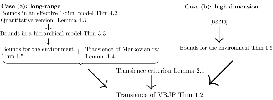
Figure 1: dependence structure of the theorems

2 Transience proof given bounds on the environment

Our transience proof uses the connection between random walks and electrical networks, cf. [LP16] for background. First we prove transience for Markovian random walks with long-range jumps.

Proof of Lemma 1.4. By [LP16, Theorem 2.11], to prove transience, it suffices to construct a unit flow of finite energy from $0$ to infinity. Following the same strategy as in the proof of [Bäu22, Theorem 1.1], we consider the pairwise disjoint annuli $B_{k}=((-2^{k},2^{k}]^{d}\setminus(-2^{k-1},2^{k-1}]^{d})\cap{\mathbb{Z}}^{d}$ for $k\in{\mathbb{N}}$ and $B_{0}=\{0\}^{d}$. We observe $|B_{k}|\geq 2^{kd}$ for $k\in{\mathbb{N}}_{0}$. Note that for $i\in B_{k}$, $j\in B_{k+1}$, we have $\|i-j\|_{\infty}\leq 2^{k+2}$ and since $w$ is decreasing and satisfies the lower bound (1.5), it holds

$$W_{ij}=w(\|i-j\|_{\infty})\geq w(2^{k+2})\geq 8\overline{W}2^{2d}\frac{(d(k+2))^{\alpha}}{2^{2d(k+2)}}\geq\overline{W}2^{-d}\frac{(k+1)^{\alpha}}{|B_{k}||B_{k+1}|}.$$ (2.1)

Given $i,j\in{\mathbb{Z}}^{d}$, we define $\theta(i,j)=-\theta(j,i)=|B_{k}|^{-1}|B_{k+1}|^{-1}$ if $i\in B_{k}$, $j\in B_{k+1}$ for some $k\in{\mathbb{N}}_{0}$, and $\theta(i,j)=0$ otherwise. Then, $\theta$ is a unit flow from $0$ to infinity, i.e., Kirchhoff’s node rule $\sum_{j\in{\mathbb{Z}}^{d}}\theta(i,j)=\delta_{0i}$ holds for all $i\in{\mathbb{Z}}^{d}$. The corresponding energy of the network with conductances $W$ is bounded as follows

$$\frac{1}{2}\sum_{i,j\in{\mathbb{Z}}^{d}}\frac{\theta(i,j)^{2}}{W_{ij}}=\sum_{k\in{\mathbb{N}}_{0}}\sum_{i\in B_{k}}\sum_{j\in B_{k+1}}\frac{|B_{k}|^{-2}|B_{k+1}|^{-2}}{W_{ij}}\leq\frac{2^{d}}{\overline{W}}\sum_{k\in{\mathbb{N}}_{0}}(k+1)^{-\alpha}<\infty$$ (2.2)

because $\alpha>1$.   

To prove transience for VRJP, we apply the following criterion for random walks in random conductances. The idea for its proof is due to Christophe Sabot and Pierre Tarrès (proof of [ST15, Cor. 4] and private communication).

Lemma 2.1 (Transience criterion)

Consider an undirected connected graph $G=(\Lambda,E_{\Lambda})$, not necessarily of finite degree, a vertex $0\in\Lambda$, and an increasing sequence $\Lambda_{N}\uparrow\Lambda$ of finite vertex sets containing $0$. Let $G_{N}=(\Lambda_{N}\cup\{\rho\},E_{N})$, where $\rho$ is an additional wiring point and $G_{N}$ is obtained from $G$ by first restricting it to $\Lambda_{N}$ and then taking wired boundary conditions.

Consider a stochastic process $X=(X_{n})_{n\in{\mathbb{N}}_{0}}$ on $G=(\Lambda,E_{\Lambda})$ starting in $0$ and taking only nearest-neighbor jumps. We assume that for each $N$, the law of the process before it hits $\Lambda\setminus\Lambda_{N}$ equals the annealed law of a random walk in some random conductances $c_{e}=c_{e}^{(N)}>0$, $e\in E_{N}$, on $G_{N}$ before it hits $\rho$. The law of $(c_{e}^{(N)})_{e\in E_{N}}$ may depend on $N$. We denote the expectation averaging over the conductances by ${\mathbb{E}}^{N}$. Let $x\in\Lambda$. Assume that there are deterministic conductances $W_{e}>0$, $e\in E_{\Lambda}$, such that the following hold:

1. For all $i\in\Lambda$, one has $\sum_{e\in E_{\Lambda}:i\in e}W_{e}<\infty$.

2. The random walk on the weighted graph $(G,W)$ is transient.

3. There is a constant $K_{x}>0$ such that for all $N\in{\mathbb{N}}$ and all $e\in E_{N}$

   $$\sum_{f\in E_{N}:x\in f}{\mathbb{E}}^{N}\left[\frac{c_{f}}{c_{e}}\right]\leq\frac{K_{x}}{W_{e}},$$ (2.3)

   where $W_{i\rho}=W_{i\rho}^{(N)}$ is defined via the wired boundary conditions as in (1.2).

Let $\mathcal{R}^{N}(W,x\leftrightarrow\rho)$ denote the effective resistance between $x$ and $\rho$ in the network $G_{N}$ with deterministic conductances $W=(W_{e})_{e\in E_{N}}$. Then, the expected number of visits in $x$ of $X$ before exiting $\Lambda_{N}$ is bounded by $K_{x}\mathcal{R}^{N}(W,x\leftrightarrow\rho)$, which is bounded uniformly in $N$. As a consequence, the expected number of visits of $x$ by the process $X$ on $G$ is finite.

Proof. Let $E_{\Lambda}^{\mathrm{rw}}$ denote the expectation with respect to the process $X$ on $G$. Let $P_{c}^{N}$ and $E^{N}_{c}$ be the probability measure and expectation, respectively, underlying the Markovian random walk $X$ on $G_{N}$ in given conductances $c$ starting in $0$. Let $\tau_{x}^{+}$ denote the first return time to $x$ and $\tau_{\rho}$ the hitting time of $\rho$. The expected number of visits to $x$ equals

$$E_{\Lambda}^{\mathrm{rw}}\left[\sum_{n=0}^{\infty}1_{\{X_{n}=x\}}\right]= \lim_{N\to\infty}{\mathbb{E}}^{N}\left[E_{c}^{N}\left[\sum_{n=0}^{\infty}1_{\{X_{n}=x,n<\tau_{\rho}\}}\right]\right].$$ (2.4)

Let $N$ be large enough that $x\in\Lambda_{N}$. Since $c_{e}^{(N)}>0$ for all $e$, the random walk hits $x$ $P_{c}^{N}$-a.s. and the number of visits to $x$ before hitting $\rho$ in fixed conductances $c$ is geometric with mean

$$E_{c}^{N}\left[\sum_{n=0}^{\infty}1_{\{X_{n}=x,n<\tau_{\rho}\}}\right]=P_{c}^{N}(\tau_{\rho}<\tau_{x}^{+})^{-1}=c(x)\mathcal{R}^{N}(c,x\leftrightarrow\rho),$$ (2.5)

where $c(x)=\sum_{f\in E_{N}:x\in f}c_{f}$ and $\mathcal{R}^{N}(c,x\leftrightarrow\rho)$ denotes the effective resistance between $x$ and $\rho$ in the network $G_{N}$ with conductances $c$; the expression of the escape probability in terms of the effective resistance is described in [LP16, formula (2.5)]. By [LP16, formula (2.7)], there is a unit flow $\theta=(\theta(i,j))_{i,j\in\Lambda_{N}:\{i,j\}\in E_{N}}$ from $x$ to $\rho$ in this network, i.e. $\theta(i,j)=-\theta(j,i)$, $\sum_{j\in\Lambda_{N}:\{i,j\}\in E_{N}}\theta(i,j)=\delta_{ix}-\delta_{i\rho}$, such that the effective resistance in the network $G_{N}$ with deterministic conductances $W$ is given by

$$\mathcal{R}^{N}(W,x\leftrightarrow\rho)=\sum_{\{i,j\}\in E_{N}}W_{ij}^{-1}\theta(i,j)^{2}.$$ (2.6)

By Thomson’s principle [LP16, Section 2.4], with the same flow $\theta$, we obtain an upper bound for the effective resistance with random conductances

$$\mathcal{R}^{N}(c,x\leftrightarrow\rho)\leq\sum_{\{i,j\}\in E_{N}}c_{ij}^{-1}\theta(i,j)^{2}.$$ (2.7)

Using assumption (2.3), we obtain the following bound for the expected number of visits in $x$ before exiting $\Lambda_{N}$

$${\mathbb{E}}^{N} \left[E_{c}^{N}\left[\sum_{n=0}^{\infty}1_{\{X_{n}=0,n<\tau_{\rho}\}}\right]\right]={\mathbb{E}}^{N}[c(x)\mathcal{R}^{N}(c,x\leftrightarrow\rho)]$$

$$\leq\sum_{\{i,j\}\in E_{N}}\sum_{\begin{subarray}{c}f\in E_{N}:\\ x\in f\end{subarray}}{\mathbb{E}}^{N}\left[\frac{c_{f}}{c_{ij}}\right]\theta(i,j)^{2}\leq K_{x}\sum_{\{i,j\}\in E_{N}}W_{ij}^{-1}\theta(i,j)^{2}$$

$$=K_{x}\mathcal{R}^{N}(W,x\leftrightarrow\rho)\uparrow_{N\to\infty}K_{x}\mathcal{R}(W,x\leftrightarrow\infty)$$ (2.8)

with a finite limit $\mathcal{R}(W,x\leftrightarrow\infty)$ because of the transience assumption. In particular, the estimate in (2.8) is uniform in $N$. Finally, (2.4) allows us to conclude.   

Using the bounds in Theorems 1.5 and 1.6, we apply the criterion from Lemma 2.1 to deduce transience of VRJP.

Proof of Theorem 1.2. We use Model 1.1 on ${\mathbb{Z}}^{d}$ with the weights $W_{ij}$, $i,j\in{\mathbb{Z}}^{d}$, and the boxes $\Lambda_{N}=\{0,\ldots,2^{N}-1\}^{d}$ replaced by shifted boxes $\tilde{\Lambda}_{N}=\Lambda_{N}+(a_{N},\ldots,a_{N})\uparrow{\mathbb{Z}}^{d}$ such that $0\in\tilde{\Lambda}_{N}$. In Model 1.1(b) only edges $\{i,j\}$ with $W_{ij}>0$ are included in the edge set. We apply Lemma 2.1 with $\tilde{\Lambda}_{N}\uparrow\Lambda={\mathbb{Z}}^{d}$. Let $G_{N}=(\tilde{\Lambda}_{N}\cup\{\rho\},E_{N})$ and $h_{i}=W_{i\rho}=W_{i\rho}^{(N)}$ be the graph and pinning with wired boundary conditions as in this lemma. By [ST15, Theorem 2], the discrete-time process associated with the VRJP on $G_{N}$ starting at $\rho$ has the same distribution as the random walk in random conductances $c_{ij}=W_{ij}e^{u_{i}+u_{j}}$, $i,j\in\tilde{\Lambda}_{N}\cup\{\rho\}$, on $G_{N}$, where $u_{i}$, $i\in\tilde{\Lambda}_{N}$, are distributed according to the law $\nu^{\tilde{\Lambda}_{N}}_{W,h}$ given in (1.3). Changing the starting point from $\rho$ to 0, one may take the same random conductances $W_{ij}e^{u_{i}+u_{j}}$, but with respect to the modified measure $e^{u_{0}}\,d\nu^{\tilde{\Lambda}_{N}}_{W,h}$ having the density $e^{u_{0}-u_{\rho}}=e^{u_{0}}$ with respect to $\nu^{\tilde{\Lambda}_{N}}_{W,h}$. This can be seen from formula (1.3) using the shift $\tilde{u}_{i}=u_{i}-u_{0}$ and noting that a factor $e^{-u_{0}}$ is replaced by $e^{-u_{\rho}}$ when changing the product $\prod_{i\in\Lambda_{N}}e^{-u_{i}}$ to $\prod_{i\in\Lambda_{N}\cup\{\rho\}\setminus\{0\}}e^{-u_{i}}$.

We verify the assumptions 1-3 of Lemma 2.1. Assumption 1 holds by hypothesis (1.4). Assumption 2 is true for long-range weights by Lemma 1.4. For Model 1.1(b) it follows from Rayleigh’s monotonicity principle [LP16, Section 2.4] and transience of nearest-neighbor simple random walk in dimensions $d\geq 3$. Finally, Assumption 3 is verified as follows. Let $N\in{\mathbb{N}}$. The expectation ${\mathbb{E}}^{N}$ in Lemma 2.1 is with respect to the environment for the VRJP starting in $0$, not in $\rho$. Hence, given $x\in\Lambda_{N}$ and $e=\{i,j\}\in E_{N}$, it remains to estimate

$$\sum_{\begin{subarray}{c}f\in E_{N}:\\ x\in f\end{subarray}}\!\!{\mathbb{E}}^{N}\left[\frac{c_{f}}{c_{e}}\right]=\!\!\sum_{\begin{subarray}{c}f\in E_{N}:\\ x\in f\end{subarray}}\!{\mathbb{E}}^{\tilde{\Lambda}_{N}}_{W,h}\left[\frac{c_{f}}{c_{e}}e^{u_{0}}\right]=\!\!\sum_{k\in(\tilde{\Lambda}_{N}\cup\{\rho\})\setminus\{x\}}\!\frac{W_{xk}}{W_{ij}}{\mathbb{E}}^{\tilde{\Lambda}_{N}}_{W,h}\left[\frac{e^{u_{x}+u_{k}}}{e^{u_{i}+u_{j}}}e^{u_{0}}\right].$$ (2.9)

In Model 1.1(a), let $\overline{W}\geq{\overline{W}_{1}}$ with ${\overline{W}_{1}}=5{\overline{W}_{3}}/\log_{2}6$ as in (4.18) and (4.19) and $c_{1}\geq(\log_{2}6)/{\overline{W}_{3}}$ as in Theorem 1.5. In particular, $c_{1}{\overline{W}_{1}}\geq 5$. In Model 1.1(b), let $\overline{W}\geq{\overline{W}_{1}}$ with ${\overline{W}_{1}}=\max\{{\overline{W}_{2}},10^{8}\}$ and ${\overline{W}_{2}}$ as in Theorem 1.6, which implies $\frac{1}{2}\overline{W}^{1/8}\geq 5$. We apply Hölder’s inequality and the estimate $e^{\pm 5u}\leq(2\cosh u)^{5}$ to obtain

$${\mathbb{E}}^{\tilde{\Lambda}_{N}}_{W,h}[e^{u_{x}+u_{k}-u_{i}-u_{j}+u_{0}}] \leq{\mathbb{E}}^{\tilde{\Lambda}_{N}}_{W,h}[e^{5u_{x}}]^{\frac{1}{5}}{\mathbb{E}}^{\tilde{\Lambda}_{N}}_{W,h}[e^{5u_{k}}]^{\frac{1}{5}}{\mathbb{E}}^{\tilde{\Lambda}_{N}}_{W,h}[e^{-5u_{i}}]^{\frac{1}{5}}{\mathbb{E}}^{\tilde{\Lambda}_{N}}_{W,h}[e^{-5u_{j}}]^{\frac{1}{5}}{\mathbb{E}}^{\tilde{\Lambda}_{N}}_{W,h}[e^{5u_{0}}]^{\frac{1}{5}}$$

$$\leq\prod_{l\in\{x,k,i,j,0\}}{\mathbb{E}}^{\tilde{\Lambda}_{N}}_{W,h}[(2\cosh u_{l})^{5}]^{\frac{1}{5}}\leq 2^{11}.$$ (2.10)

In case (a), the last inequality follows from the bound (1.8) in Theorem 1.5 with $m=5$ and $\kappa=1$, actually even with $2^{6}$ instead of $2^{11}$. Note that the theorem is applied to the translated box $\tilde{\Lambda}_{N}$ rather than the original box $\Lambda_{N}$, using translational invariance of the weights. In case (b) the last estimate in (2.10) follows from Theorem 1.6. Substituting the bound (2.10) in (2.9), we obtain

$$\sum_{f\in E_{N}:x\in f}{\mathbb{E}}^{N}\left[\frac{c_{f}}{c_{e}}\right]\leq 2^{11}\sum_{k\in(\tilde{\Lambda}_{N}\cup\{\rho\})\setminus\{x\}}\frac{W_{xk}}{W_{ij}}=\frac{K_{x}}{W_{ij}},$$ (2.11)

with $K_{x}=2^{11}\sum_{k\in{\mathbb{Z}}^{d}\setminus\{x\}}W_{xk}<\infty$. Having checked all its hypotheses, we apply Lemma 2.1 to conclude that the expected number of visits to $x$ is finite. By assumption (1.4), the constants $K_{x}$ are uniformly bounded in $x$. The limit $\mathcal{R}(W,x\leftrightarrow\infty)=\lim_{N\to\infty}\mathcal{R}^{N}(W,x\leftrightarrow\rho)$ does not depend on the choice of the boxes $\tilde{\Lambda}_{N}\uparrow{\mathbb{Z}}^{d}$. Finally, if the weights $W_{ij}$ are translation invariant, it does not depend on $x$.   

3 Bounding environments

3.1 High dimension

We need the following monotonicity result for VRJP in the weights.

Fact 3.1 (Poudevigne’s monotonicity theorem [PA22, Theorem 6])

Consider two families of non-negative edge weights and pinnings $W^{+},h^{+}$ and $W^{-},h^{-}$ on the same vertex set $\Lambda$, satisfying $W^{+}\geq W^{-}$ and $h^{+}\geq h^{-}$ componentwise. For any convex function $f:[0,\infty)\to{\mathbb{R}}$ and all $i\in\Lambda$, one has

$${\mathbb{E}}^{\Lambda}_{W^{+},h^{+}}\left[f(e^{u_{i}})\right]\leq{\mathbb{E}}^{\Lambda}_{W^{-},h^{-}}\left[f(e^{u_{i}})\right].$$ (3.1)

In particular, for $m\geq 1$,

$${\mathbb{E}}^{\Lambda}_{W^{+},h^{+}}\left[(\cosh u_{i})^{m}\right]\leq{\mathbb{E}}^{\Lambda}_{W^{-},h^{-}}\left[(\cosh u_{i})^{m}\right].$$ (3.2)

Recall that $\rho$ denotes the wiring point. In Poudevigne’s notation, the joint law of $G^{\pm}(\rho,i)/G^{\pm}(\rho,\rho)$, $i\in\Lambda$, from [PA22, Theorem 6] coincides with the joint law of $e^{u_{i}}$, $i\in\Lambda$, with respect to $\nu^{\Lambda}_{W^{\pm},h^{\pm}}$. Taking the convex function $f(x)=2^{-m}(x+x^{-1})^{m}$, $m\geq 1$, yields $f(e^{u_{i}})=(\cosh u_{i})^{m}$ and hence (3.2).
Using this monotonicity, we derive the bounds for the environment in Model 1.1(b).

Proof of Theorem 1.6. Take ${\overline{W}_{2}}$ large enough, to be specified below, and let $\overline{W}\geq{\overline{W}_{2}}$. By assumption, $W_{ij}\geq\overline{W}1_{\{\|i-j\|_{2}=1\}}=:W^{\rm nn}_{ij}$ and $h_{i}=W_{i\rho}\geq W^{\rm nn}_{i\rho}=:h^{\rm nn}_{i}$ where $W^{\rm nn}_{i\rho}$ is defined as in (1.2). Therefore, for $m\geq 1$, by Fact 3.1 above, we can compare our model with weights $W,h$ with the nearest neighbor model with weights $W^{\rm nn},h^{\rm nn}$:

$${\mathbb{E}}^{\Lambda_{N}}_{W,h}\left[(\cosh u_{i})^{m}\right]\leq{\mathbb{E}}^{\Lambda_{N}}_{W^{\rm nn},h^{\rm nn}}\left[(\cosh u_{i})^{m}\right].$$ (3.3)

We observe that $\cosh a\leq 2\cosh(a-b)\cosh b$ for all $a,b\in{\mathbb{R}}.$ Therefore, for any $j\in\partial\Lambda_{N},$ using Cauchy-Schwarz, we obtain

$${\mathbb{E}}^{\Lambda_{N}}_{W^{\rm nn},h^{\rm nn}}\left[(\cosh u_{i})^{m}\right] \leq 2^{m}{\mathbb{E}}^{\Lambda_{N}}_{W^{\rm nn},h^{\rm nn}}\left[(\cosh(u_{i}-u_{j}))^{m}(\cosh u_{j})^{m}\right]$$

$$\leq 2^{m}{\mathbb{E}}^{\Lambda_{N}}_{W^{\rm nn},h^{\rm nn}}\left[(\cosh(u_{i}-u_{j}))^{2m}\right]^{\frac{1}{2}}{\mathbb{E}}^{\Lambda_{N}}_{W^{\rm nn},h^{\rm nn}}\left[(\cosh u_{j})^{2m}\right]^{\frac{1}{2}}.$$ (3.4)

Assuming now that ${\overline{W}_{2}}$ is so large that ${\overline{W}_{2}}\geq 2^{8}$ and [DSZ10, Theorem 1] is applicable, we have

$${\mathbb{E}}^{\Lambda_{N}}_{W^{\rm nn},h^{\rm nn}}\left[(\cosh(u_{i}-u_{j}))^{2m}\right]\leq 2$$ (3.5)

for all $m\in[1,\frac{1}{2}\overline{W}^{\frac{1}{8}}]\neq\emptyset.$ Note that this result holds for any choice of the pinning and in any dimension $d\geq 3.$
The next bound uses the estimate (5.9) from Lemma 5.2 below which is valid on any finite graph and is a consequence of supersymmetry. Since $j\in\partial\Lambda_{N}$ we have $W_{j\rho}\geq\overline{W}$ and hence using $u_{\rho}=0$ and (5.9) in the first inequality we get

$${\mathbb{E}}^{\Lambda_{N}}_{W^{\rm nn},h^{\rm nn}}\left[(\cosh u_{j})^{2m}\right] ={\mathbb{E}}^{\Lambda_{N}}_{W^{\rm nn},h^{\rm nn}}\left[(\cosh(u_{j}-u_{\rho}))^{2m}\right]$$

$$\leq\frac{1}{1-\frac{2m}{W_{j\rho}}}\leq\frac{1}{1-\frac{2m}{\overline{W}}}\leq 2,$$ (3.6)

where in the last step we used $2m\leq\overline{W}^{\frac{1}{8}}$ and $\overline{W}\geq 2^{8/7}$. The result (1.10) now follows for $m\in[1,\frac{1}{2}\overline{W}^{\frac{1}{8}}]$. For $0\leq m<1$, Jensen’s inequality and the already proven claim for $m=1$ yield

$${\mathbb{E}}^{\Lambda_{N}}_{W,h}\left[(\cosh u_{i})^{m}\right]\leq{\mathbb{E}}^{\Lambda_{N}}_{W,h}\left[\cosh u_{i}\right]^{m}\leq 2^{2m}\leq 2^{m+1}.$$ (3.7)

 

Note that in the case $m\geq 1$ it would suffice to do this proof for $d=3.$ Indeed for $d\geq 4$ one can embed ${\mathbb{Z}}^{3}$ in ${\mathbb{Z}}^{d}$ and use Poudevigne’s monotonicity (Fact 3.1) together with the result in $d=3.$

3.2 Long-range interaction

To prove Theorem 1.5 we compare a box in the Euclidean lattice with long range interactions with the corresponding box in a hierarchical lattice as follows.

Model 3.2 (Complete graph with hierarchical interactions)

Fix $N\in{\mathbb{N}}$. We consider the vertex set consisting of the set of leaves $\Lambda_{N}=\{0,1\}^{N}$ of the binary tree ${\mathcal{T}}=\cup_{n=0}^{N}\{0,1\}^{n}$. For $i=(i_{0},\ldots,i_{N-1}),j=(j_{0},\ldots,j_{N-1})\in\{0,1\}^{N}$, the hierarchical distance is defined by $d_{H}(i,j)=\min(\{l\in\{0,\ldots,N-1\}:\,i_{k}=j_{k}\text{ for all }k\geq l\}\cup\{N\})$; it is the distance to the least common ancestor in ${\mathcal{T}}$. We endow ${\mathcal{T}}$ with hierarchical weights

$$W_{ij}^{H}=w^{H}(d_{H}(i,j)),\quad i,j\in\Lambda_{N},i\neq j,$$ (3.8)

with a weight function $w^{H}:{\mathbb{N}}\to(0,\infty)$ and uniform pinning $W_{i\rho}=h^{H}>0$ for all $i\in\Lambda$.

An illustration of ${\mathcal{T}}$ is given in Figure 2.

Figure 2: hierarchical graph for $N=3$ together with the pinning point. In Model 3.2 any two leaves of the binary tree have a positive interaction.

The main technical result of this paper is the following theorem.

Theorem 3.3 (Bounds on the environment – hierarchical case)

Let $\kappa\in(0,1]$ and $\alpha>3$. Take ${\overline{W}_{3}}$ large enough and $c_{1}>0$ small enough; explicit bounds are given in Lemma 4.3. Let $\overline{W}\geq{\overline{W}_{3}}$. Consider Model 3.2 and assume that the weight function $w^{H}$ and the pinning $h^{H}$ satisfy

$$w^{H}(r)\geq 8\overline{W}2^{-2r}r^{\alpha}\text{ for }r\in{\mathbb{N}},\quad h^{H}\geq 2\overline{W}2^{-N}(N+1)^{\alpha}.$$ (3.9)

Then, for all $i\in\Lambda_{N}$ and all $m\in[0,c_{1}\overline{W}]$, one has

$${\mathbb{E}}_{W^{H},h^{H}}^{\Lambda_{N}}[(\cosh u_{i})^{m}]\leq 1+\kappa.$$ (3.10)

As a consequence, for all $i,j\in\Lambda_{N}$ and all $m\in[0,\frac{1}{2}c_{1}\overline{W}]$, one has

$${\mathbb{E}}_{W^{H},h^{H}}^{\Lambda_{N}}[(\cosh(u_{i}-u_{j}))^{m}]\leq 2^{m}(1+\kappa).$$ (3.11)

The proof of this result is based on the connection between the random environment for VRJP and the non-linear supersymmetric hyperbolic sigma model $H^{2|2}.$ This model is introduced in Section 4. Sections 5–7 are devoted to the proof.

Fix $N\in{\mathbb{N}}$ and take the box $\Lambda_{N}:=\{0,1,\ldots,2^{N}-1\}^{d}$.

Figure 3: illustration of the map $\phi$ for $N=2$ and $d=2$

In order to compare $\Lambda_{N}$ with $\{0,1\}^{Nd}$, we define (cf. Fig.3)

$$\phi:\Lambda_{N}\to\{0,1\}^{Nd},\quad\phi(i_{0},\ldots,i_{d-1})=(z_{0},\ldots,z_{Nd-1}),$$ (3.12)

where $z_{n}\in\{0,1\}$ denotes the $\lfloor n/d\rfloor$-th digit in the binary expansion $i_{l}=\sum_{k=0}^{N-1}z_{dk+l}2^{k}$, with $l=n\,\mod\,d$. The map $\phi$ is a bijection. The elements of $\{0,1\}^{Nd}$ can be visualized as the leaves of a binary tree. On this set, the hierarchical distance, i.e. the distance to the least common ancestor in the binary tree, is given by

$$d_{H}(z,z^{\prime})=\min(\{n\in\{0,\ldots,Nd-1\}:\,z_{m}=z_{m}^{\prime}\text{ for all }m\geq n\}\cup\{Nd\}).$$ (3.13)

On $\Lambda_{N}$, the natural definition of hierarchical distance would be $\lceil d_{H}(\phi(i),\phi(j))/d\rceil$. With this choice in Figure 3 any two points in the same small box would have distance 1 from each other, while points in different boxes would have distance 2. In the following lemma, we compare the maximum norm distance with the hierarchical distance.

Lemma 3.4 (Comparison of $d_{H}$ and $\|\cdot\|_{\infty}$)

For all $i,j\in\Lambda_{N}$, one has

$$2\cdot 2^{d_{H}(\phi(i),\phi(j))/d}\geq 2^{\lceil d_{H}(\phi(i),\phi(j))/d\rceil}>\|i-j\|_{\infty}.$$ (3.14)

Proof. For $i=j$, the claim is true. We take $i\neq j$ in $\Lambda_{N}$ and set $z=\phi(i)$, $z^{\prime}=\phi(j)$, and $r=d_{H}(z,z^{\prime})$. One has

$$\|i-j\|_{\infty}=\max_{0\leq l\leq d-1}|i_{l}-j_{l}|=\max_{0\leq l\leq d-1}\left|\sum_{k=0}^{N-1}(z_{dk+l}-z_{dk+l}^{\prime})2^{k}\right|.$$ (3.15)

The only non-zero contributions in the above sum come from $k$ satisfying $dk+l\leq r-1$ which implies $k\leq(r-1)/d$. It follows that

$$\|i-j\|_{\infty} \leq\max_{0\leq l\leq d-1}\sum_{k=0}^{\lfloor(r-1)/d\rfloor}|z_{dk+l}-z_{dk+l}^{\prime}|2^{k}$$

$$\leq\sum_{k=0}^{\lfloor(r-1)/d\rfloor}2^{k}<2^{\lfloor(r-1)/d\rfloor+1}=2^{\lceil r/d\rceil},$$ (3.16)

where we use $|z_{dk+l}-z_{dk+l}^{\prime}|\leq 1$.   

Next, we show how the bound on the environment for the Euclidean box with long-range interactions follows from Theorem 3.3.

Proof of Theorem 1.5. For $m\geq 1$, we apply Fact 3.1 to compare the Euclidean long-range model, i.e. Model 1.1(a), but restricted to the box $\Lambda_{N}$ with wired boundary conditions, with a hierarchical model defined on the same box. Remember that in the Euclidean model, we take long-range weights $W^{+}_{ij}:=W_{ij}=w(\|i-j\|_{\infty})$ as in Model 1.1(a) and pinning $h^{+}_{j}:=h_{j}$ given in (1.7). In the hierarchical model, we take weights

$$W^{-}_{ij}:=W^{H}_{ij}=w^{H}(d_{H}(\phi(i),\phi(j)))\text{ with }w^{H}(r):=w(2^{\lceil r/d\rceil})$$ (3.17)

and uniform pinning given by $h^{-}:=h^{H}:=\min_{j\in\Lambda_{N}}h_{j}$. By Lemma 3.4 and monotonicity of $w$,

$$W_{ij}=w(\|i-j\|_{\infty})\geq w\left(2^{\lceil d_{H}(\phi(i),\phi(j))/d\rceil}\right)=W^{H}_{ij},\quad h_{i}\geq h^{H},$$ (3.18)

for $i,j\in\Lambda_{N}$. By monotonicity (3.2), for all $i\in\Lambda_{N}$ and $m\geq 1$, one has

$${\mathbb{E}}^{\Lambda_{N}}_{W,h}\left[(\cosh u_{i})^{m}\right]\leq{\mathbb{E}}^{\Lambda_{N}}_{W^{H},h^{H}}\left[(\cosh u_{i})^{m}\right].$$ (3.19)

We identify $\Lambda_{N}$ with $\{0,1\}^{Nd}$ via the bijection $\phi:\Lambda_{N}\to\{0,1\}^{Nd}$ from (3.12). As a result we obtain Model 3.2 with $N$ replaced by $Nd$. With $\overline{W}$ specified below, we apply Theorem 3.3 with

$$w^{H}(r)= w(2^{\lceil r/d\rceil})\geq 8\overline{W}2^{2d}\frac{(d\lceil r/d\rceil)^{\alpha}}{2^{2d\lceil r/d\rceil}}\geq 8\overline{W}2^{2d}\frac{r^{\alpha}}{2^{2d(1+r/d)}}=8\overline{W}2^{-2r}r^{\alpha},$$ (3.20)

where we used (1.5). We estimate the pinning using that $w$ is decreasing

$$h^{H}=\min_{i\in\Lambda_{N}}h_{i}=\min_{i\in\Lambda_{N}}\sum_{j\in{\mathbb{Z}}^{d}\setminus\Lambda_{N}}w(\|i-j\|_{\infty})\geq\sum_{\begin{subarray}{c}j\in{\mathbb{Z}}^{d}:\\ 2^{N}\leq\|j\|_{\infty}<2^{N+1}\end{subarray}}w(\|j\|_{\infty})\geq w(2^{N+1})\sum_{\begin{subarray}{c}j\in{\mathbb{Z}}^{d}:\\ 2^{N}\leq\|j\|_{\infty}<2^{N+1}\end{subarray}}1.$$ (3.21)

The last sum has at least $2^{(N+1)d}$ summands, which is a lower bound on the cardinality of the set $\{z\in{\mathbb{Z}}:\,2^{N}\leq|z|<2^{N+1}\}\times\{j\in{\mathbb{Z}}^{d-1}:\,\|j\|_{\infty}<2^{N+1}\}$. Hence, we obtain

$$h^{H}\geq 2^{(N+1)d}w(2^{N+1})\geq 2^{(N+1)d}\cdot 8\overline{W}2^{2d}\frac{(Nd+d)^{\alpha}}{2^{2(N+1)d}}\geq 2\overline{W}2^{-Nd}(Nd+1)^{\alpha}.$$ (3.22)

Thus, assumption (3.9) of Theorem 3.3 is satisfied with $N$ replaced by $Nd$ and the estimate (1.8) follows for $m\in[1,c_{1}\overline{W}]$ and $\overline{W}\geq{\overline{W}_{3}}$ with $c_{1}$, ${\overline{W}_{3}}$ fulfilling $c_{1}{\overline{W}_{3}}>1$ taken from Lemma 4.3. For $m<1$, Jensen’s inequality and the proven claim for $m=1$ yield

$${\mathbb{E}}^{\Lambda_{N}}_{W,h}\left[(\cosh u_{i})^{m}\right]\leq{\mathbb{E}}^{\Lambda_{N}}_{W,h}\left[\cosh u_{i}\right]^{m}\leq(1+\kappa)^{m}\leq 1+\kappa.$$ (3.23)

To deduce (1.9) from (1.8), we observe that $\cosh(u_{i}-u_{j})\leq 2\cosh u_{i}\cosh u_{j}$. By Cauchy-Schwarz, we obtain

$${\mathbb{E}}_{W,h}^{\Lambda_{N}} [(\cosh(u_{i}-u_{j}))^{m}]\leq 2^{m}{\mathbb{E}}_{W,h}^{\Lambda_{N}}[(\cosh u_{i})^{m}(\cosh u_{j})^{m}]$$

$$\leq 2^{m}{\mathbb{E}}_{W,h}^{\Lambda_{N}}[(\cosh u_{i})^{2m}]^{1/2}{\mathbb{E}}_{W,h}^{\Lambda_{N}}[(\cosh u_{j})^{2m}]^{1/2}\leq 2^{m}(1+\kappa).$$ (3.24)

 

3.3 Uniform integrability

Proof of Lemma 1.3. Note that for some $m>1$ one has ${\mathbb{E}}^{\Lambda_{N}}_{W,h}[(\cosh u_{i})^{m}]\leq 2$ for all boxes $\Lambda_{N}\subset{\mathbb{Z}}^{d}$ of side length $2^{N}.$ This follows from Theorem 1.5 together with translation invariance in the case of Model 1.1(a) and from Theorem 1.6 in case of Model 1.1(b). Given an arbitrary finite set $\Lambda^{\prime}\subset{\mathbb{Z}}^{d}$ there exists a box $\Lambda_{N}$ of side length $2^{N}$ with $\Lambda^{\prime}\subseteq\Lambda_{N}$ for $N$ large enough. We endow both of them with wired boundary conditions. Given $i\in\Lambda^{\prime},$ according to [SZ19, Theorem 1] one can couple $u_{i}^{(\Lambda^{\prime})}$ and $u_{i}^{(\Lambda_{N})}$ such that $e^{u_{i}^{(\Lambda^{\prime})}},e^{u_{i}^{(\Lambda_{N})}}$ is a one-step martingale. Note that $e^{u}$ is called $\psi$ in [SZ19]. Since $(\cosh u)^{m}$ is a convex function of $e^{u}$ for $m>1,$ Jensen’s inequality gives ${\mathbb{E}}^{\Lambda^{\prime}}_{W,h}[(\cosh u_{i})^{m}]\leq{\mathbb{E}}^{\Lambda_{N}}_{W,h}[(\cosh u_{i})^{m}]\leq 2$. Using $e^{u_{i}}\leq 2\cosh u_{i}$, the claim follows.   

4 Non-linear supersymmetric hyperbolic sigma model

It remains to prove the bounds on the environment in the hierarchical model given in Theorem 3.3. This requires a careful analysis of the random environment which is described by the $H^{2|2}$ model.

4.1 The model

The supersymmetric hyperbolic sigma $H^{2|2}$ model was introduced by Zirnbauer [Zir91] in the context of quantum diffusion. It can be seen as a statistical mechanical spin model where the spins take values in the supermanifold $H^{2|2}.$ This is the hyperboloid $H^{2}=\{(x,y,z)\in{\mathbb{R}}^{3}:\ x^{2}+y^{2}-z^{2}=-1,\ z>0\}$ extended by two Grassmann, i.e. anticommuting, variables $\xi,\eta$ with the constraint $z^{2}=1+x^{2}+y^{2}+2\xi\eta.$ For more mathematical background see [Swa20], [DMR22, Appendix] and [DSZ10]. Changing to horospherical coordinates $(x,y,\xi,\eta)\mapsto(u,s,\overline{\psi},\psi),$ cf. [DSZ10, eq. (2.7)], where $u,s$ are real and $\overline{\psi},\psi$ are Grassmann variables, the model can be defined as follows.

We consider a finite undirected graph with vertex set $\Lambda$ and edge set $E_{\Lambda}$. Every edge $e=\{i,j\}\in E_{\Lambda}$ is given a positive weight $W_{ij}=W_{ji}=W_{e}>0$. To every vertex $i\in\Lambda$, we associate a pinning strength $h_{i}\geq 0$ in such a way that every connected component of the graph contains at least one vertex $i$ with $h_{i}>0$. It is convenient to treat pinning and interaction in a unified way. Therefore, we extend the vertex set $\Lambda$ by a special vertex $\rho\notin\Lambda$ called “pinning point” or “wiring point”. In addition, we introduce pinning edges connecting the pinning point with the other vertices. Since we will study correlations between any pair of points, we will also add edges connecting vertices without direct interaction. Therefore, we consider the undirected complete graph $G=(\Lambda\cup\{\rho\},E)$ without direct loops. Every edge $e\in E$ is given a weight $W_{e}\geq 0$ as follows. For $e\in E_{\Lambda}$, $W_{e}>0$ is the weight defined above. The weight of pinning edges $e=\{i,\rho\}$, $i\in\Lambda$, is defined to be the pinning strength $W_{e}=h_{i}$. All other edges $e$ are given weight $W_{e}=0$. The subgraph consisting of edges with positive weights is denoted by

$$G_{+}=(\Lambda\cup\{\rho\},E_{+}),\quad\text{where }E_{+}:=\{e\in E:W_{e}>0\}.$$ (4.1)

Note that $E_{+}$ consists of $E_{\Lambda}$ and the pinning edges with positive weight, and our assumption on the pinning is equivalent to require that the graph $G_{+}$ is connected.

We assign to every vertex $i$ two real-valued variables $u_{i}$ and $s_{i}$ and two Grassmann variables $\overline{\psi}_{i}$ and $\psi_{i}$. We set $u_{\rho}=s_{\rho}:=0=:\overline{\psi}_{\rho}=\psi_{\rho}$. Following [DSZ10, eq. (2.9-2.10)], for all $e=\{i,j\}$ with $i,j\in\Lambda\cup\{\rho\}$ with $i\neq j$, we set

$$B_{ij}= B_{e}=B_{e}(u,s):=\cosh(u_{i}-u_{j})+\frac{1}{2}(s_{i}-s_{j})^{2}e^{u_{i}+u_{j}},$$ (4.2)

$$S_{ij}= S_{e}=S_{e}(u,s,\overline{\psi},\psi):=B_{e}+(\overline{\psi}_{i}-\overline{\psi}_{j})(\psi_{i}-\psi_{j})e^{u_{i}+u_{j}}.$$ (4.3)

For each vertex $i\in\Lambda$, let

$$B_{i}:=B_{i\rho}=\cosh u_{i}+\frac{1}{2}s_{i}^{2}e^{u_{i}},\quad S_{i}:=S_{i\rho}=B_{i}+\overline{\psi}_{i}\psi_{i}e^{u_{i}}.$$ (4.4)

The action of the non-linear hyperbolic sigma model in horospherical coordinates is given by, cf. [DSZ10, eq. (2.8) with $z_{i}=S_{i}$],

$$A=A(u,s,\overline{\psi},\psi):=\sum_{e\in E_{\Lambda}}W_{e}(S_{e}-1)+\sum_{i\in\Lambda}h_{i}(S_{i}-1)=\sum_{e\in E_{+}}W_{e}(S_{e}-1).$$ (4.5)

The superintegration form of the model is given by, [DSZ10, eq. (2.12-2.13)],

$$\left\langle{f}\right\rangle=\left\langle{f}\right\rangle^{\Lambda}_{W,h}:=\int_{{\mathbb{R}}^{\Lambda}\times{\mathbb{R}}^{\Lambda}}\prod_{i\in\Lambda}\frac{e^{-u_{i}}}{2\pi}\,du_{i}\,ds_{i}\,\partial_{\overline{\psi}_{i}}\partial_{\psi_{i}}\,fe^{-A}$$ (4.6)

for any function of the variables $u_{i},s_{i},\overline{\psi}_{i},\psi_{i}$ such that the integral exists. For any integrable function $f=f(u,s)$ which does not depend on the Grassmann variables, one has

$$\left\langle{f}\right\rangle={\mathbb{E}}[f]={\mathbb{E}}^{\Lambda}_{W,h}[f]:= \int_{{\mathbb{R}}^{\Lambda}\times{\mathbb{R}}^{\Lambda}}f(u,s)\,\mu^{\Lambda}_{W,h}(du\,ds),$$ (4.7)

where $\mu^{\Lambda}_{W,h}$ is the probability measure on ${\mathbb{R}}^{\Lambda}\times{\mathbb{R}}^{\Lambda}$ given by

$$\mu(du\,ds)=\mu^{\Lambda}_{W,h}(du\,ds):= e^{-\sum_{e\in E_{\Lambda}}W_{e}(B_{e}-1)-\sum_{i\in\Lambda}h_{i}(B_{i}-1)}\det D\prod_{i\in\Lambda}\frac{e^{-u_{i}}}{2\pi}\,du_{i}\,ds_{i}$$

$$= e^{-\sum_{e\in E_{+}}W_{e}(B_{e}-1)}\det D\prod_{i\in\Lambda}\frac{e^{-u_{i}}}{2\pi}\,du_{i}\,ds_{i},$$ (4.8)

and $D=D(u)=(D_{ij})_{i,j\in\Lambda}$ is the weighted Laplacian matrix on $G_{+}$ with entries

$$D_{ij}=\left\{\begin{array}[]{ll}-W_{ij}e^{u_{i}+u_{j}}&\text{if }\{i,j\}\in E_{+},\\ \sum_{k\in\Lambda:\{i,k\}\in E_{+}}W_{ik}e^{u_{i}+u_{k}}&\text{if }i=j,\\ 0&\text{otherwise.}\end{array}\right.$$ (4.12)

Note that for $i,j\in\Lambda$ the condition $\{i,j\}\in E_{+}$ is equivalent to $\{i,j\}\in E_{\Lambda}$, and that the diagonal entries can also be written in the form $D_{ii}=\sum_{k\in\Lambda:\{i,k\}\in E_{\Lambda}}W_{ik}e^{u_{i}+u_{k}}+h_{i}e^{u_{i}}$. Our connectedness assumption on the graph $G_{+}$ guarantees that the matrix $D$ is positive definite. In particular, it is invertible. The fact that $\mu^{\Lambda}_{W,h}$ is a probability measure was shown in [DSZ10] using supersymmetry. Since the $s$-variables, conditionally on $u$, are normally distributed with covariance $D^{-1}$, and by the matrix-tree theorem $\det D=\sum_{T\in\mathcal{S}}\prod_{\{i,j\}\in T}W_{ij}e^{u_{i}+u_{j}},$ the $u$-marginal of $\mu^{\Lambda}_{W,h}$ is given by (1.3). In particular, for functions depending only on $u$ the expectations with respect to $\mu^{\Lambda}_{W,h}$ and $\nu^{\Lambda}_{W,h}$ coincide, which allows us to use the same notation ${\mathbb{E}}^{\Lambda}_{W,h}$.

4.2 One-dimensional effective model

The expectation of $(\cosh u_{i})^{m}$ in the hierarchical model will be reduced to a similar expectation in an effective non-homogeneous one-dimensional model with vertex set $\Lambda_{N}:=\{1,2,\ldots,N\}$ and long-range interactions as will be shown in (7.1) below based on [DMR22, Cor. 2.3]. The vertices in this effective model correspond to length scales in the original hierarchical model. The following model describes a one-dimensional chain with inhomogeneous weights and purely nearest neighbor interactions. In the application to our hierarchical model, additional long-range interactions will be included as well, but these can be easily removed via a monotonicity result given in Lemma 5.6.

Model 4.1 (One-dimensional model with non-homogeneous interactions)

For any $N\in{\mathbb{N}}$, we consider the graph $(\Lambda_{N},E_{N})$ with vertex set $\Lambda_{N}:=\{1,2,\ldots,N\}$, undirected edge set $E_{N}=\{\{i-1,i\}:2\leq i\leq N\}$, and weights $W_{\{i-1,i\}}\geq\overline{W}i^{\alpha}$, $i\in{\mathbb{N}}$, depending on positive parameters $\overline{W}$ and $\alpha$. We consider two versions of pinning.

1. Either the pinning point $\rho$ does not belong to $\Lambda_{N}$. In this case, we take any pinning vector $h=(h_{j})_{j=1,\ldots,N}\in[0,\infty)^{N}\setminus\{0\}$.

2. Or the pinning point $\rho$ coincides with one of the vertices $\Lambda_{N}$, e.g. $\rho=N$. Here, we take the pinning vector $h=(h_{j})_{j=1,\ldots,N,j\neq\rho}$ with $h_{j}=W_{j\rho}$.

The following theorem is the main technical result of this paper. It gives bounds on this family of non-homogeneous one-dimensional models, possibly with additional long-range interactions. We consider two sets of edges $E^{\prime}$ and $E^{\prime\prime}$. Edges in $E^{\prime}$ are nearest-neighbor, while edges in $E^{\prime\prime}$ are typically not, see remarks below the theorem. For any edge $e\in E_{N}$, we write $e=\{x_{e},y_{e}\}$ with $x_{e}<y_{e}$.

Theorem 4.2 (Bounds on the environment – effective one-dimensional case)

Let $\kappa\in(0,1]$, $\alpha>3$ and $\gamma\geq 0$ with $\alpha-\gamma>3$. There exist ${\overline{W}_{3}}={\overline{W}_{3}}(\kappa,\alpha,\gamma)>0$ and $c_{1}=c_{1}(\kappa,\alpha,\gamma)>0$ such that for all $\overline{W}\geq{\overline{W}_{3}}$ the following hold for Model 4.1.

Let $E^{\prime},E^{\prime\prime}$ be disjoint subsets of the edge set $\{\{x,y\}\subseteq\Lambda_{N}:x\neq y\}$ of the complete graph over $\Lambda_{N}$. We assume that every $e\in E^{\prime}$ is a nearest neighbor edge: $y_{e}-x_{e}=1$, i.e. $E^{\prime}\subseteq E_{N}$, and for any two different $e,\tilde{e}\in E^{\prime}\cup E^{\prime\prime}$ the open intervals $(x_{e},y_{e})$ and $(x_{\tilde{e}},y_{\tilde{e}})$ are disjoint. Set $m_{x}:=c_{1}\overline{W}x^{\gamma}$ for all $x\in{\mathbb{N}}$. Then, for all exponents $m_{e}$ satisfying $0\leq m_{e}<W_{e}$ for $e\in E^{\prime}$ and $0\leq m_{e}\leq m_{x_{e}}$ for $e\in E^{\prime\prime}$, we have

$${\mathbb{E}}_{W,h}^{\Lambda_{N}}\left[\prod_{e\in E^{\prime}}B_{e}^{m_{e}}\cdot\prod_{e\in E^{\prime\prime}}B_{e}^{m_{e}}\right]\leq\prod_{e\in E^{\prime}}\frac{1}{1-\frac{m_{e}}{W_{e}}}\cdot(1+\kappa)^{|E^{\prime\prime}|},$$ (4.13)

uniformly in $N$. If $0\leq m_{e}\leq m_{x_{e}}$ for all $e\in E^{\prime}\cup E^{\prime\prime}$, one has

$${\mathbb{E}}_{W,h}^{\Lambda_{N}}\left[\prod_{e\in E^{\prime}}B_{e}^{m_{e}}\cdot\prod_{e\in E^{\prime\prime}}B_{e}^{m_{e}}\right]\leq(1+\kappa)^{|E^{\prime}|+|E^{\prime\prime}|},$$ (4.14)

again uniformly in $N$. In particular, for all $e=\{x,y\}$ with $x,y\in\Lambda_{N}$ with $x<y$ and all $m\in[0,m_{x}]$, one has

$${\mathbb{E}}_{W,h}^{\Lambda_{N}}[(\cosh(u_{x}-u_{y})^{m}]\leq{\mathbb{E}}_{W,h}^{\Lambda_{N}}[B_{e}^{m}]\leq 1+\kappa.$$ (4.15)

In the case P1 of pinning, all estimates are also uniform in the pinning $h$.

The same results hold if we add arbitrarily many additional non-nearest neighbor edges $e$ with arbitrary non-negative weights $W_{e}\geq 0$ to the graph $(\Lambda_{N},E_{N})$.

Let us explain the different roles of $E^{\prime}$ and $E^{\prime\prime}$: Edges $e\in E^{\prime}$ can be treated in a simple way using supersymmetric Ward identities (see equation (5.9)) resulting in the bound $(1-m_{e}/W_{e})^{-1}$; however, these edges need to have a positive weight $W_{e}>0$ with $m_{e}/W_{e}<1$. For edges with small positive $W_{e}$ this provides a bound only for exponents $m_{e}$ so small that it is not useful anymore. For edges with zero weight the strategy does not work at all. This type of edges forms the set $E^{\prime\prime}$. The corresponding estimate is the most technical part of this work and requires the weights of nearest-neighbor edges to be large enough. This technical construction may also be applied to nearest-neighbor edges, but the corresponding bound is weaker, i.e. $1+\kappa$ instead of $(1-m_{e}/W_{e})^{-1}$.

Lemma 4.3 (Quantitative version of Theorem 4.2)

In Theorem 4.2, one may choose $\gamma\in[0,\alpha-3)$,

$${\overline{W}_{3}}={\overline{W}_{3}}(\kappa,\alpha,\gamma)=-\frac{1}{2{c_{2}}}\log\frac{\kappa}{36},\quad c_{1}=\frac{{c_{2}}}{\log 2}$$ (4.16)

with the constant

$${c_{2}}={c_{2}}(\kappa,\alpha,\gamma)=\min\left\{\frac{2\log 2}{3e^{\sqrt{2}\frac{\alpha-\gamma-1}{\alpha-\gamma-3}}}\kappa,\frac{1}{16}\right\}.$$ (4.17)

With theses choices, $m_{x}\geq c_{1}{\overline{W}_{3}}\geq\log_{2}6>1$. For

$$\overline{W}\geq{\overline{W}_{1}}:=\frac{5}{\log_{2}6}{\overline{W}_{3}}>{\overline{W}_{3}},$$ (4.18)

one has $m_{x}\geq 5$. In the case $\gamma=0$ and $\kappa=1$, we have

$${\overline{W}_{3}}=\max\left\{16\log 6,\frac{3}{2}e^{\sqrt{2}\frac{\alpha-1}{\alpha-3}}\log_{2}6\right\},\quad{\overline{W}_{1}}=\max\left\{80\log 2,\frac{15}{2}e^{\sqrt{2}\frac{\alpha-1}{\alpha-3}}\right\}.$$ (4.19)

Strategy of the proof

The expectation of $\prod_{e\in E^{\prime}\cup E^{\prime\prime}}B_{e}^{m_{e}}$ is estimated using a partition of unity. For some summands in this partition we use an iteration of the bound $B_{ij}\leq 2B_{ik}B_{kj}.$ After this additional expansion any summand in the partition “protects” some factors $B_{ij}^{m}$ with a cut-off function $\chi_{ij}$ and does not protect other factors. Factors with the complement of the protection $1-\chi_{ij}$ are estimated using Chebychev’s inequality. The expectation of the remaining product is estimated by supersymmetric Ward identities and bounds on determinants which rely on the protections.

5 Notation and main technical ingredients

In this section, $G=(\Lambda\cup\{\rho\},E)$ is the complete graph with weights $W_{e}\geq 0$, $e\in E$, such that $G_{+}$ is connected, cf. formula (4.1).

5.1 A Ward identity and some applications

In this section, we use the $H^{2|2}$-model with Grassmann variables still present. Note that real functions of even elements of the Grassmann algebra are defined as formal Taylor series in the Grassmann variables, which are nilpotent. For example, for an edge $e=\{i,j\}$, the expression $f(S_{e})$ is defined by $f(S_{e})=f(B_{e}+n_{e}):=f(B_{e})+f^{\prime}(B_{e})n_{e}$ with $n_{e}=n_{ij}=(\overline{\psi}_{i}-\overline{\psi}_{j})(\psi_{i}-\psi_{j})e^{u_{i}+u_{j}}$. This Taylor expansion stops after the first order term because $n_{e}^{2}=0$ by the anticommutativity of the Grassmann variables.
We will use the following localization result from [DSZ10].

Lemma 5.1 (Ward identity)

Let $f_{e}:[1,\infty)\to{\mathbb{R}}$, $e\in E$, be a family of continuously differentiable functions such that each $f_{e}$ and its derivative $f_{e}^{\prime}$ are bounded by polynomials. Then it holds

$$\left\langle{\prod_{e\in E}f_{e}(S_{e})}\right\rangle=\prod_{e\in E}f_{e}(1).$$ (5.1)

Proof. This is a special case of the localization result in [DSZ10, Prop. 2 in the appendix]. The key points are that any $S_{e}$ is annihilated by the supersymmetry operator used in the proposition and $S_{ij}=1$ holds whenever $u_{k}=s_{k}=\overline{\psi}_{k}=\psi_{k}=0$ for $k\in\{i,j\}$.   

Notation

The following notation will be technically convenient. The two vertices incident to an edge $e\in E$ are denoted by $e_{+}$ and $e_{-}$. This gives every edge a direction $e_{+}\to e_{-}$, which has no physical meaning, but is used for bookkeeping purposes. Let

$$F\in\{-1,0,1\}^{\Lambda\times E},\quad F_{k,e}=1_{\{e_{+}=k\}}-1_{\{e_{-}=k\}}\quad\text{for }k\in\Lambda,\,e\in E$$ (5.2)

denote the signed incidence matrix of $G$ with $\rho$ removed, but keeping the pinning edges. We consider the diagonal matrix

$$\mathcal{W}=\mathcal{W}(u):=\operatorname{diag}(\mathcal{W}_{e},e\in E)\in{\mathbb{R}}^{E\times E}\quad\text{with}\quad\mathcal{W}_{e}:=W_{e}e^{u_{e_{+}}+u_{e_{-}}}.$$ (5.3)

With these notations, we reformulate the weighted Laplacian matrix $D$ from (4.12) as

$$D=F\mathcal{W}F^{t}\in{\mathbb{R}}^{\Lambda\times\Lambda}.$$ (5.4)

We will also need the following matrices:

$$Q=Q^{G}(u,s):=\operatorname{diag}(Q_{e},e\in E)\quad\text{with}\quad Q_{e}:=\frac{e^{u_{e_{+}}+u_{e_{-}}}}{B_{e}(u,s)},$$ (5.5)

$${\mathcal{G}}={\mathcal{G}}^{G}_{W}(u,s):=\sqrt{Q}F^{t}D^{-1}F\sqrt{Q}\in{\mathbb{R}}^{E\times E}.$$ (5.6)

Let $m_{e}\geq 0$, $e\in E$. We set

$$M:=\operatorname{diag}(m_{e},e\in E).$$ (5.7)

Lemma 5.2

The following hold:

$${\mathbb{E}}\left[\prod_{e\in E}B_{e}^{m_{e}}\cdot\det(\operatorname{Id}-M\mathcal{G})\right]=1.$$ (5.8)

If in addition $0\leq m_{e}<W_{e}$ for $e\in E_{+}$ defined in (4.1) and $m_{e}=0$ otherwise, the equality implies

$${\mathbb{E}}\left[\prod_{e\in E_{+}}(\cosh(u_{e_{+}}-u_{e_{-}}))^{m_{e}}\right]\leq{\mathbb{E}}\left[\prod_{e\in E_{+}}B_{e}^{m_{e}}\right]\leq\prod_{e\in E_{+}}\frac{1}{1-\frac{m_{e}}{W_{e}}}.$$ (5.9)

Proof. Ward identity (5.1) with $f_{e}(x)=x^{m_{e}}$ reads

$$\left\langle{\prod_{e\in E}S_{e}^{m_{e}}}\right\rangle=1.$$ (5.10)

We calculate for $e=\{i,j\}$, using $(\overline{\psi}^{t}F_{\cdot e}F^{t}_{e\cdot}\psi)^{2}=0$,

$$S_{e}^{m_{e}}= B_{e}^{m_{e}}+m_{e}B_{e}^{m_{e}-1}(\overline{\psi}_{i}-\overline{\psi}_{j})(\psi_{i}-\psi_{j})e^{u_{i}+u_{j}}$$

$$= B_{e}^{m_{e}}\left(1+\frac{m_{e}}{B_{e}}e^{u_{i}+u_{j}}\overline{\psi}^{t}F_{\cdot e}F^{t}_{e\cdot}\psi\right)=B_{e}^{m_{e}}\left(1+\overline{\psi}^{t}F_{\cdot e}m_{e}Q_{e}F^{t}_{e\cdot}\psi\right)$$

$$= B_{e}^{m_{e}}\exp\left(\overline{\psi}^{t}F_{\cdot e}m_{e}Q_{e}F^{t}_{e\cdot}\psi\right).$$ (5.11)

Hence, taking a product over $e$,

$$1=\left\langle{\prod_{e\in E}S_{e}^{m_{e}}}\right\rangle= \left\langle{\exp\left(\overline{\psi}^{t}FMQF^{t}\psi\right)\prod_{e\in E}B_{e}^{m_{e}}}\right\rangle.$$ (5.12)

The Grassmann part in the action $A$ in (4.5) is given by

$$\sum_{\{i,j\}\in E_{+}}W_{ij}(\overline{\psi}_{i}-\overline{\psi}_{j})(\psi_{i}-\psi_{j})e^{u_{i}+u_{j}} =\sum_{e\in E_{+}}\overline{\psi}^{t}F_{\cdot e}\mathcal{W}_{e}F^{t}_{e\cdot}\psi$$

$$=\overline{\psi}^{t}F\mathcal{W}F^{t}\psi=\overline{\psi}^{t}D\psi.$$ (5.13)

Using the definition (4.8) of $\mu$, we can rewrite (5.12) as

$$1= \int\limits_{{\mathbb{R}}^{\Lambda}\times{\mathbb{R}}^{\Lambda}}\prod_{i\in\Lambda}\partial_{\overline{\psi}_{i}}\partial_{\psi_{i}}\exp(-\overline{\psi}^{t}(D-FMQF^{t})\psi)\prod_{e\in E}B_{e}^{m_{e}}\,\frac{\mu(du\,ds)}{\det D}$$

$$= {\mathbb{E}}\left[\prod_{e\in E}B_{e}^{m_{e}}\frac{\det(D-FMQF^{t})}{\det D}\right].$$ (5.14)

Using the identity $\det(\operatorname{Id}+AB)=\det(\operatorname{Id}+BA)$, which holds for arbitrary rectangular matrices $A\in{\mathbb{R}}^{m\times n}$, $B\in{\mathbb{R}}^{n\times m}$, and the fact $MQ=\sqrt{Q}M\sqrt{Q}$, we obtain

$$\frac{\det(D-FMQF^{t})}{\det D}= \det(\operatorname{Id}-D^{-1}FMQF^{t})$$

$$= \det(\operatorname{Id}-M\sqrt{Q}F^{t}D^{-1}F\sqrt{Q})=\det(\operatorname{Id}-M{\mathcal{G}}),$$ (5.15)

where in the second expression the identity matrix $\operatorname{Id}$ is indexed by vertices, while in the third and fourth expression it is indexed by edges. We conclude claim (5.8).

Assume now $0\leq m_{e}<W_{e}$ for $e\in E_{+}$ and $m_{e}=0$ otherwise. We calculate

$$\det(\operatorname{Id}-M{\mathcal{G}})\det D= \det(D-FMQF^{t})=\det(F(\mathcal{W}-MQ)F^{t}).$$ (5.16)

Note that $F(\mathcal{W}-MQ)F^{t}$ is a discrete Laplacian with weights $\mathcal{W}_{e}-m_{e}Q_{e}$ rather than $\mathcal{W}_{e}$. Edges in $E_{+}$ have a positive weight $\mathcal{W}_{e}-m_{e}Q_{e}=\mathcal{W}_{e}(1-\frac{m_{e}}{W_{e}B_{e}})>0$ since $B_{e}\geq 1$. Using the matrix tree theorem and writing ${\mathcal{T}}$ for the set of spanning trees of the graph $G_{+}$, we rewrite the last determinant as follows

$$\det(F(\mathcal{W}-MQ)F^{t})=\sum_{T\in{\mathcal{T}}}\prod_{e\in T}(\mathcal{W}_{e}-m_{e}Q_{e})=\sum_{T\in{\mathcal{T}}}\prod_{e\in T}\mathcal{W}_{e}\left(1-\frac{m_{e}}{W_{e}B_{e}}\right).$$ (5.17)

For each $T\in{\mathcal{T}}$, we have

$$\prod_{e\in T}\left(1-\frac{m_{e}}{W_{e}B_{e}}\right)\geq\prod_{e\in E_{+}}\left(1-\frac{m_{e}}{W_{e}B_{e}}\right)\geq\prod_{e\in E_{+}}\left(1-\frac{m_{e}}{W_{e}}\right).$$ (5.18)

Therefore, we obtain

$$\det(F(\mathcal{W}-MQ)F^{t})\geq\prod_{e\in E_{+}}\left(1-\frac{m_{e}}{W_{e}}\right)\sum_{T\in{\mathcal{T}}}\prod_{e\in T}\mathcal{W}_{e}=\prod_{e\in E_{+}}\left(1-\frac{m_{e}}{W_{e}}\right)\det D.$$ (5.19)

It follows from (5.16) that

$$\det(\operatorname{Id}-M{\mathcal{G}})\geq\prod_{e\in E_{+}}\left(1-\frac{m_{e}}{W_{e}}\right).$$ (5.20)

Inserting this in (5.8) and using $\cosh(u_{e_{+}}-u_{e_{-}})\leq B_{e}$, the claim (5.9) follows.   

Unfortunately, the symmetric matrix $\operatorname{Id}-\sqrt{M}{\mathcal{G}}\sqrt{M}$ might not be positive definite when $m_{e}>0$ for some edge $e\notin E_{+}$. This is an obstruction to extend the bound (5.9) to cases where $m_{e}>0$ but $W_{e}=0$ can occur. We can still obtain an analogue of (5.9) if we restrict the expectation to a smaller set of configurations by introducing a family $(\chi_{e})_{e\in E}$ of protection functions. For $e\in E$, let $\delta_{e}\in(0,\infty]$ and

$$\chi_{e}:{\mathbb{R}}\to{\mathbb{R}},\quad\chi_{e}=1_{(-\infty,1+\delta_{e})}$$ (5.21)

be the indicator function of the interval $(-\infty,1+\delta_{e})$. Let $\chi_{e}^{n}:{\mathbb{R}}\to[0,1]$, $n\in{\mathbb{N}}$, be smooth approximations of $\chi_{e}$ such that $\chi_{e}^{n}(b)=1$ for $b\leq 1$, $\chi_{e}^{n}(b)=0$ for $b\geq 1+\delta_{e}$, $b\mapsto\chi_{e}^{n}(b)$ is decreasing, and $\chi_{e}^{n}\uparrow\chi_{e}$ as $n\uparrow\infty$. Note that for $\delta_{e}=\infty$, one has $\chi_{e}\equiv 1$. In this case, we choose $\chi_{e}^{n}\equiv 1$ for all $n$.

As a replacement for the hypothesis $0\leq m_{e}<W_{e}$ of bound (5.9), we use the following assumption, which needs to be checked in a model-dependent way in concrete cases:

Assumption 5.3

We assume that the choice of the parameters $\delta_{e}$, $e\in E$, depending on the weights $W_{e}$ and the exponents $m_{e}$, $e\in E$, is such that $D(u)>FMQ(u,s)F^{t}$ holds on the set of configurations

$$U:=\{(u,s)\in{\mathbb{R}}^{\Lambda}\times{\mathbb{R}}^{\Lambda}:B_{e}(u,s)<1+\delta_{e}\text{ for all }e\in E\}.$$ (5.22)

Note that $1_{U}=\prod_{e\in E}\chi_{e}(B_{e})$.

The following lemma states an analogue of equality (5.8). We do not have a universal analogue of bound (5.9) since bounds on the determinant $\det(\operatorname{Id}-M{\mathcal{G}})$ need to be derived for the individual models.

Lemma 5.4

Under the Assumption 5.3 one has

$$1\geq{\mathbb{E}}\left[\prod_{e\in E}B_{e}^{m_{e}}\cdot\prod_{e\in E}\chi_{e}(B_{e})\cdot\det(\operatorname{Id}-M{\mathcal{G}})\right].$$ (5.23)

Proof. The proof follows the lines of the proof of Lemma 5.2 with some additional complications due to the presence of the cutoff functions. From Ward identity (5.1) with $f_{e}(x)=x^{m_{e}}\chi_{e}^{n}(x)$ using $\chi_{e}^{n}(1)=1$ we know for all $n\in{\mathbb{N}}$:

$$\left\langle{\prod_{e\in E}(S_{e}^{m_{e}}\chi_{e}^{n}(S_{e}))}\right\rangle=1.$$ (5.24)

Note that the Grassmann derivatives contained in the expectation involve derivatives of the cutoff functions. This is why we need to replace the indicator functions $\chi_{e}$ by smooth approximations $\chi_{e}^{n}$. At the end we will take the limit $n\to\infty$. We expand $\chi_{e}^{n}(S_{e})$ for $e=\{i,j\}\in E$ in the Grassmann variables:

$$\chi_{e}^{n}(S_{e})= \chi_{e}^{n}(B_{e})+(\chi_{e}^{n})^{\prime}(B_{e})e^{u_{i}+u_{j}}\overline{\psi}^{t}F_{\cdot e}F^{t}_{e\cdot}\psi$$ (5.25)

Since $\chi_{e}^{n}\geq 0$, all $b$ with $\chi_{e}^{n}(b)=0$ are local minima and hence satisfy $(\chi_{e}^{n})^{\prime}(b)=0$. Hence $\chi_{e}^{n}(B_{e})=0$ implies $\chi_{e}^{n}(S_{e})=0$. Thus $S_{e}^{m_{e}}\chi_{e}^{n}(S_{e})=S_{e}^{m_{e}}\chi_{e}^{n}(S_{e})1_{\{\chi_{e}^{n}(B_{e})>0\}}$. On the event $\{\chi_{e}^{n}(B_{e})>0\}$, using $(\overline{\psi}^{t}F_{\cdot e}F^{t}_{e\cdot}\psi)^{2}=0$ again, we obtain

$$\chi_{e}^{n}(S_{e})= \chi_{e}^{n}(B_{e})\left(1+\overline{\psi}^{t}F_{\cdot e}R_{e}F^{t}_{e\cdot}\psi\right)=\chi_{e}^{n}(B_{e})\exp(\overline{\psi}^{t}F_{\cdot e}R_{e}F^{t}_{e\cdot}\psi)$$ (5.26)

with $R_{e}:=e^{u_{i}+u_{j}}(\chi_{e}^{n})^{\prime}(B_{e})/\chi_{e}^{n}(B_{e})$. Combining this expression with the expansion (5.11) of $S_{e}^{m_{e}}$, it follows

$$S_{e}^{m_{e}}\chi_{e}^{n}(S_{e})= B_{e}^{m_{e}}\chi_{e}^{n}(B_{e})\exp\left(\overline{\psi}^{t}F_{\cdot e}[m_{e}Q_{e}+R_{e}]F^{t}_{e\cdot}\psi\right).$$ (5.27)

The following calculations are performed on the event $U_{n}:=\{\chi_{e}^{n}(B_{e})>0\text{ for all }e\in E\}$. Note that $U_{n}\uparrow U$ as $n\to\infty$. Let $R:=\operatorname{diag}(R_{e},e\in E)$. One has

$$\prod_{e\in E}(S_{e}^{m_{e}}\chi_{e}^{n}(S_{e}))= \prod_{e\in E}(B_{e}^{m_{e}}\chi_{e}^{n}(B_{e}))\exp(-\overline{\psi}^{t}(-F(MQ+R)F^{t})\psi).$$ (5.28)

Since $\chi_{e}^{n}$ is non-negative and decreasing, $(\chi_{e}^{n})^{\prime}/\chi_{e}^{n}\leq 0$. Consequently,

$$-a^{t}FRF^{t}a=-\sum_{e=\{i,j\}\in E}e^{u_{i}+u_{j}}\frac{(\chi_{e}^{n})^{\prime}(B_{e})}{\chi_{e}^{n}(B_{e})}(a_{i}-a_{j})^{2}\geq 0$$ (5.29)

for all $a\in{\mathbb{R}}^{\Lambda}$ and hence the matrix $-FRF^{t}$ is positive semidefinite.

The Grassmann part in the Boltzmann factor $e^{-A}$ is given by $\exp(-\overline{\psi}^{t}D\psi)$. Hence, using that the product $\prod_{e\in E}\chi_{e}^{n}(B_{e})$ vanishes on $U_{n}^{c}$ and the value of the indicator function $1_{U_{n}}$ depends only on the real variables $u$ and $s$, but not on the Grassmann variables $\overline{\psi}$ and $\psi$, we can rewrite (5.24) as follows

$$1 =\left\langle{\prod_{e\in E}(B_{e}^{m_{e}}\chi_{e}^{n}(B_{e}))e^{-\overline{\psi}^{t}(-F(MQ+R)F^{t})\psi}}\right\rangle$$

$$=\int\limits_{{\mathbb{R}}^{\Lambda}\times{\mathbb{R}}^{\Lambda}}\prod_{e\in E}(B_{e}^{m_{e}}\chi_{e}^{n}(B_{e}))\prod_{i\in\Lambda}\partial_{\overline{\psi}_{i}}\partial_{\psi_{i}}e^{-\overline{\psi}^{t}(D-F(MQ+R)F^{t})\psi}\,\frac{\mu(du\,ds)}{\det D}$$

$$={\mathbb{E}}\left[\prod_{e\in E}(B_{e}^{m_{e}}\chi_{e}^{n}(B_{e}))\frac{\det(D-F(MQ+R)F^{t})}{\det D}\right].$$ (5.30)

Since $U_{n}\subseteq U$, $D-FMQF^{t}>0$ holds on $U_{n}$ by Assumption 5.3. Together with $-FRF^{t}\geq 0$ this yields, cf. (5.1)

$$\frac{\det(D-F(MQ+R)F^{t})}{\det D}\geq\frac{\det(D-FMQF^{t})}{\det D}=\det(\operatorname{Id}-M{\mathcal{G}})>0$$ (5.31)

and we conclude

$$1\geq {\mathbb{E}}_{W}\left[\prod_{e\in E}(B_{e}^{m_{e}}\chi_{e}^{n}(B_{e}))\det(\operatorname{Id}-M{\mathcal{G}})\right]$$ (5.32)

for all $n$. Taking the limit $n\to\infty$ the result follows by monotone convergence.   

5.2 Bounds on determinants

The following lemma is useful to verify Assumption 5.3.

Lemma 5.5

1. The following two statements are equivalent:

   $$\sqrt{M}{\mathcal{G}}\sqrt{M}<\operatorname{Id}\qquad\Leftrightarrow\qquad D>FMQF^{t}.$$ (5.33)

2. If $W_{e}\geq m_{e}$ for all $e\in E$ and the graph $(\Lambda\cup\{\rho\},\{e\in E:W_{e}>m_{e}\})$ is connected, then the two equivalent conditions in (5.33) hold.

Proof. For the first part, we use the following fact from linear algebra: for any possibly rectangular real-valued matrix $A$ the statements $AA^{t}<\operatorname{Id}$ and $A^{t}A<\operatorname{Id}$ are equivalent. This follows from the fact that the sets of non-zero eigenvalues of $AA^{t}$ and of $A^{t}A$ coincide. We apply this fact to $A=D^{-1/2}F\sqrt{M}\sqrt{Q}$. Note that $\sqrt{M}\sqrt{Q}=\sqrt{Q}\sqrt{M}$ because $M$ and $Q$ are diagonal matrices. We calculate

$$A^{t}A=\sqrt{M}\sqrt{Q}F^{t}D^{-1}F\sqrt{Q}\sqrt{M}=\sqrt{M}{\mathcal{G}}\sqrt{M};$$ (5.34)

thus $A^{t}A<\operatorname{Id}$ is equivalent to the first statement in (5.33). On the other hand, using the equality

$$AA^{t}=D^{-1/2}FMQF^{t}D^{-1/2}$$ (5.35)

and $D^{t}=D$, we obtain that $AA^{t}<\operatorname{Id}$ is equivalent to $D^{-1/2}(D-FMQF^{t})D^{-1/2}>0$, which is equivalent to the second statement in (5.33).

For the second part, assume that $W_{e}\geq m_{e}$ for all $e\in E$. Then it follows that $W_{e}\geq m_{e}/B_{e}$ because $B_{e}\geq 1$ and consequently

$$\mathcal{W}_{e}=W_{e}e^{u_{e_{+}}+u_{e_{-}}}\geq\frac{m_{e}}{B_{e}}e^{u_{e_{+}}+u_{e_{-}}}=m_{e}Q_{e}.$$ (5.36)

Moreover, the above inequality is strict if $W_{e}>m_{e}$. We assume now that the graph $\tilde{G}:=(\Lambda\cup\{\rho\},\{e\in E:W_{e}>m_{e}\})$ is connected. Let $x\in{\mathbb{R}}^{\Lambda}\setminus\{0\}$ and set $x_{\rho}=0$. Then, there is $i\in\Lambda$ with $x_{i}\neq 0$. Since $i$ and $\rho$ are connected by $\tilde{G}$ there is an edge $e\in E$ with $W_{e}>m_{e}$ and $x_{e_{+}}\neq x_{e_{-}}$, i.e. $(F^{t}x)_{e}\neq 0$. We conclude

$$0<(\mathcal{W}_{e}-m_{e}Q_{e})(F^{t}x)_{e}^{2}\leq x^{t}F(\mathcal{W}-MQ)F^{t}x.$$ (5.37)

Hence, $D=F\mathcal{W}F^{t}>FMQF^{t}$.   

The next result shows some monotonicity of $\det(\operatorname{Id}-M{\mathcal{G}})$ with respect to $W_{e}$ and $m_{e}$ and will be used to compare $\det(\operatorname{Id}-M{\mathcal{G}})$ for $G$ and the graph obtained from $G$ by removing some edges.

Lemma 5.6 (Monotonicity of the determinant in the parameters)

Let $(m_{e})_{e\in E}$, $(W_{e})_{e\in E}\in[0,\infty)^{E}$ and $(m_{e}^{\prime})_{e\in E},(W_{e}^{\prime})_{e\in E}\in[0,\infty)^{E}$ be families of parameters such that $m_{e}\leq m_{e}^{\prime}$ and $W_{e}\geq W_{e}^{\prime}$ for all $e\in E$. Assume that the second one (the primed one) satisfies Assumption 5.3. Then, the first one satisfies it as well.

Moreover, let the matrices $M,{\mathcal{G}}$ and $M^{\prime},{\mathcal{G}}^{\prime}$ be defined according to (5.6) and (5.7) with the first and second family of parameters, respectively. Then, one has on the event $U$

$$0<\det(\operatorname{Id}-M^{\prime}{\mathcal{G}}^{\prime})\leq\det(\operatorname{Id}-M{\mathcal{G}}).$$ (5.38)

Proof. Set $\mathcal{W}_{e}^{\prime}:=W_{e}^{\prime}e^{u_{e_{+}}+u_{e_{-}}}$, $\mathcal{W}^{\prime}:=\operatorname{diag}(\mathcal{W}_{e}^{\prime},e\in E)$, and $D^{\prime}:=F\mathcal{W}^{\prime}F^{t}$. By assumption, we know $D^{\prime}=F\mathcal{W}^{\prime}F^{t}>FM^{\prime}QF^{t}$ on the event $U$. The assumptions $m_{e}\leq m_{e}^{\prime}$ and $W_{e}\geq W_{e}^{\prime}$, $e\in E$, imply $D=F\mathcal{W}F^{t}\geq F\mathcal{W}^{\prime}F^{t}=D^{\prime}>FM^{\prime}QF^{t}\geq FMQF^{t}$, hence $D>FMQF^{t}$ and $D>FM^{\prime}QF^{t}$ hold on the event $U$ as well and thus Assumption 5.3 is satisfied.

For the second claim, on the event $U$, we observe that the last two inequalities and our assumption imply $\sqrt{M}{\mathcal{G}}\sqrt{M}<\operatorname{Id}$, $\sqrt{M^{\prime}}{\mathcal{G}}^{\prime}\sqrt{M^{\prime}}<\operatorname{Id}$, and $\sqrt{M^{\prime}}{\mathcal{G}}\sqrt{M^{\prime}}<\operatorname{Id}$ by Lemma 5.5. The last inequality and $M\leq M^{\prime}$ yield $0\leq\sqrt{{\mathcal{G}}}M\sqrt{{\mathcal{G}}}\leq\sqrt{{\mathcal{G}}}M^{\prime}\sqrt{{\mathcal{G}}}<\operatorname{Id}$, cf. first two lines in the proof of Lemma 5.5. Since $D\geq D^{\prime}$, we infer

$${\mathcal{G}}=\sqrt{Q}F^{t}D^{-1}F\sqrt{Q}\leq\sqrt{Q}F^{t}(D^{\prime})^{-1}F\sqrt{Q}={\mathcal{G}}^{\prime},$$ (5.39)

which implies $0\leq\sqrt{M^{\prime}}{\mathcal{G}}\sqrt{M^{\prime}}\leq\sqrt{M^{\prime}}{\mathcal{G}}^{\prime}\sqrt{M^{\prime}}<\operatorname{Id}$. We conclude

$$\det (\operatorname{Id}-M{\mathcal{G}})=\det(\operatorname{Id}-\sqrt{{\mathcal{G}}}M\sqrt{{\mathcal{G}}})\geq\det(\operatorname{Id}-\sqrt{{\mathcal{G}}}M^{\prime}\sqrt{{\mathcal{G}}})$$

$$=\det(\operatorname{Id}-\sqrt{M^{\prime}}{\mathcal{G}}\sqrt{M^{\prime}})\geq\det(\operatorname{Id}-\sqrt{M^{\prime}}{\mathcal{G}}^{\prime}\sqrt{M^{\prime}})=\det(\operatorname{Id}-M^{\prime}{\mathcal{G}}^{\prime})>0$$ (5.40)

because the determinant is monotonically increasing on the set of positive definite matrices.   

We now compare the determinants associated to two graphs $G$ and $G^{\prime}$, where $G^{\prime}$ is obtained from $G$ by splitting some vertices and edges in several ones. In other words, $G$ is obtained from $G^{\prime}$ by identifying vertices according to some map $k$.

Lemma 5.7 (Separating vertices)

Let $G=(\Lambda\cup\{\rho\},E)$ and $G^{\prime}=(\Lambda^{\prime}\cup\{\rho\},E^{\prime})$ be two complete graphs, endowed with families of weights $W_{e}$, $W_{e^{\prime}}^{\prime}\geq 0$, $e\in E$, $e^{\prime}\in E^{\prime}$, such that $G_{+}$ and $G_{+}^{\prime}$ are connected, cf. (4.1). We take parameters $m_{e}$, $m_{e^{\prime}}^{\prime}\geq 0$, $e\in E$, $e^{\prime}\in E^{\prime}$, and we assume that there exists a surjective map $k:\Lambda^{\prime}\cup\{\rho\}\to\Lambda\cup\{\rho\}$ such that $k^{-1}(\{\rho\})=\{\rho\}$ and

$$W_{e}=\sum_{e^{\prime}\in E^{\prime}}W_{e^{\prime}}^{\prime}1_{\{k(e^{\prime})=e\}},\quad m_{e}=\sum_{e^{\prime}\in E^{\prime}}m_{e^{\prime}}^{\prime}1_{\{k(e^{\prime})=e\}},$$ (5.41)

where for $e^{\prime}=\{i,j\}$ we set $k(e^{\prime}):=\{k(i),k(j)\}$. Given $u_{i}$ and $s_{i}$ for $i\in\Lambda\cup\{\rho\}$, define $u_{i}^{\prime}:=u_{k(i)}$, $s_{i}^{\prime}:=s_{k(i)}$ for $i\in\Lambda^{\prime}\cup\{\rho\}$. Let ${\mathcal{G}}(u,s),{\mathcal{G}}^{\prime}(u^{\prime},s^{\prime}),M$, and $M^{\prime}$ be defined as in (5.6) and (5.7). If $\sqrt{M^{\prime}}{\mathcal{G}}^{\prime}(u^{\prime},s^{\prime})\sqrt{M^{\prime}}\leq(1-\theta)\operatorname{Id}$ for a given $\theta\in(0,1)$, then $\sqrt{M}{\mathcal{G}}(u,s)\sqrt{M}\leq(1-\theta)\operatorname{Id}$ and one has

$$\det(\operatorname{Id}-M{\mathcal{G}}(u,s))\geq\det(\operatorname{Id}-M^{\prime}{\mathcal{G}}^{\prime}(u^{\prime},s^{\prime})).$$ (5.42)

The assumption $k^{-1}(\{\rho\})=\{\rho\}$ guarantees that $u_{i}^{\prime}=u_{\rho}$ if and only if $i=\rho$ and the same holds for $s_{i}^{\prime}$.

Proof. Throughout the proof, all matrices with prime belong to the weighted graph $(G^{\prime},W^{\prime})$ and are evaluated at $u^{\prime},s^{\prime}$. The claim (5.42) is equivalent to

$$\det(\operatorname{Id}-\sqrt{M}{\mathcal{G}}\sqrt{M})\geq\det(\operatorname{Id}-\sqrt{M^{\prime}}{\mathcal{G}}^{\prime}\sqrt{M^{\prime}}).$$ (5.43)

We define the matrix $K\in\{0,1\}^{\Lambda\times\Lambda^{\prime}}$ by $K_{jj^{\prime}}=1$ iff $k(j^{\prime})=j$. The proof uses the following two auxiliary identities

$$KF^{\prime}\mathcal{W}^{\prime}(u^{\prime})(F^{\prime})^{t}K^{t}= F\mathcal{W}(u)F^{t},$$ (5.44)

$$KF^{\prime}M^{\prime}Q^{\prime}(u^{\prime},s^{\prime})(F^{\prime})^{t}K^{t}= FMQ(u,s)F^{t},$$ (5.45)

which are shown in Lemma 5.8 below. We introduce

$$C:=D^{-1/2}F\sqrt{QM},\quad L:=D^{-1/2}KF^{\prime}\sqrt{Q^{\prime}M^{\prime}}.$$ (5.46)

Note that $M$ and $Q$ are diagonal and hence commute. Using (5.45) for the second equality, we calculate

$$\sqrt{M}{\mathcal{G}}\sqrt{M}=C^{t}C,\quad CC^{t}=LL^{t}.$$ (5.47)

It follows that $\sqrt{M}{\mathcal{G}}\sqrt{M}$, $LL^{t}$, and $L^{t}L$ all have the same eigenvalues including multiplicities with the possible exception of 0, and

$$\det(\operatorname{Id}-\sqrt{M}{\mathcal{G}}\sqrt{M})= \det(\operatorname{Id}-C^{t}C)=\det(\operatorname{Id}-CC^{t})$$

$$= \det(\operatorname{Id}-LL^{t})=\det(\operatorname{Id}-L^{t}L).$$ (5.48)

We will prove

$$\sqrt{M^{\prime}}{\mathcal{G}}^{\prime}\sqrt{M^{\prime}}\geq L^{t}L.$$ (5.49)

Since by assumption $\sqrt{M^{\prime}}{\mathcal{G}}^{\prime}\sqrt{M^{\prime}}\leq(1-\theta)\operatorname{Id}$, using the coincidence of eigenvalues $\neq 0$, this inequality implies $L^{t}L\leq(1-\theta)\operatorname{Id}$ and hence $\sqrt{M}{\mathcal{G}}\sqrt{M}\leq(1-\theta)\operatorname{Id}$. The claim (5.42) follows directly from (5.48) and (5.49).

To prove (5.49), we calculate $L^{t}L=\sqrt{M^{\prime}Q^{\prime}}(KF^{\prime})^{t}D^{-1}KF^{\prime}\sqrt{Q^{\prime}M^{\prime}}$. Using (5.44), we find $D=F\mathcal{W}F^{t}=KF^{\prime}\mathcal{W}^{\prime}(F^{\prime})^{t}K^{t}=KD^{\prime}K^{t}$ and thus

$$L^{t}L=\sqrt{M^{\prime}Q^{\prime}}(KF^{\prime})^{t}(KD^{\prime}K^{t})^{-1}KF^{\prime}\sqrt{Q^{\prime}M^{\prime}}.$$ (5.50)

The claim (5.49) is equivalent to

$$\sqrt{M^{\prime}Q^{\prime}}\left[(F^{\prime})^{t}(D^{\prime})^{-1}F^{\prime}\right]\sqrt{Q^{\prime}M^{\prime}}\geq\sqrt{M^{\prime}Q^{\prime}}\left[(KF^{\prime})^{t}(KD^{\prime}K^{t})^{-1}KF^{\prime}\right]\sqrt{Q^{\prime}M^{\prime}}.$$ (5.51)

To show the last inequality, it is sufficient to prove the following comparison between the matrices in brackets:

$$(F^{\prime})^{t}(D^{\prime})^{-1}F^{\prime}\geq(KF^{\prime})^{t}(KD^{\prime}K^{t})^{-1}KF^{\prime}.$$ (5.52)

We show first

$$\sqrt{\mathcal{W}^{\prime}}(F^{\prime})^{t}(D^{\prime})^{-1}F^{\prime}\sqrt{\mathcal{W}^{\prime}}\geq\sqrt{\mathcal{W}^{\prime}}(KF^{\prime})^{t}(KD^{\prime}K^{t})^{-1}KF^{\prime}\sqrt{\mathcal{W}^{\prime}}.$$ (5.53)

Let $R:=F^{\prime}\sqrt{\mathcal{W}^{\prime}}$, $\tilde{R}:=KR$. Then, $D^{\prime}=RR^{t}$ is invertible and $\tilde{R}\tilde{R}^{t}=KRR^{t}K^{t}$. The operators $R^{t}(RR^{t})^{-1}R$ and $\tilde{R}^{t}(\tilde{R}\tilde{R}^{t})^{-1}\tilde{R}$ are orthogonal projections to $\operatorname{range}R^{t}$ and $\operatorname{range}\tilde{R}^{t}$, respectively. Since $\tilde{R}^{t}=R^{t}K^{t}$, one has $\operatorname{range}\tilde{R}^{t}\subseteq\operatorname{range}R^{t}$ and consequently, $R^{t}(RR^{t})^{-1}R\geq\tilde{R}^{t}(\tilde{R}\tilde{R}^{t})^{-1}\tilde{R}$. Inserting the definitions of $R$ and $\tilde{R}$, this yields (5.53).

If $\mathcal{W}^{\prime}$ is invertible, the identity (5.52) follows directly. The set of weights $W^{\prime}=(W_{e^{\prime}}^{\prime})_{e^{\prime}\in E^{\prime}}$ such that (5.52) holds is closed in the set of all allowed weights. The set of all $W^{\prime}$ such that $\mathcal{W}^{\prime}$ is invertible is a dense subset of the set of all allowed weights. Thus, (5.52) follows.   

Next, we prove the auxiliary statements needed in the proof of Lemma 5.7. We use the same notation as in the lemma and its proof.

Lemma 5.8 (Auxiliary identities)

Under the assumptions of Lemma 5.7, the equations (5.44) and (5.45) hold.

Proof. We prove first (5.44). This can be reformulated as $D_{ij}=\sum_{i^{\prime}\in k^{-1}(\{i\}),\,j^{\prime}\in k^{-1}(\{j\})}D_{i^{\prime}j^{\prime}}^{\prime}$ for all $i,j\in\Lambda$. For $i,j\in\Lambda$, let $D_{ij}^{0}$ be the contribution to $D_{ij}$ without pinning:

$$D_{ij}=1_{\{i=j\}}\mathcal{W}_{i\rho}+D_{ij}^{0}.$$ (5.54)

In particular, $\sum_{j\in\Lambda}D_{ij}^{0}=0$ for all $i\in\Lambda$. In the same way, we write $D_{i^{\prime}j^{\prime}}^{\prime}=1_{\{i^{\prime}=j^{\prime}\}}\mathcal{W}_{i^{\prime}\rho}^{\prime}+D_{i^{\prime}j^{\prime}}^{\prime 0}$. For the pinning part we compute

$$\mathcal{W}_{i\rho}=W_{i\rho}e^{u_{i}}=\sum_{i^{\prime}\in k^{-1}(\{i\})}W_{i^{\prime}\rho}^{\prime}e^{u_{i}}=\sum_{i^{\prime}\in k^{-1}(\{i\})}\mathcal{W}_{i^{\prime}\rho}^{\prime}\quad\text{ for all }i\in\Lambda,$$ (5.55)

where we used (5.41) and $u_{i^{\prime}}^{\prime}=u_{i}$. It remains to show $D_{ij}^{0}=\sum_{i^{\prime}\in k^{-1}(\{i\}),\,j^{\prime}\in k^{-1}(\{j\})}D_{i^{\prime}j^{\prime}}^{\prime 0}$ for all $i,j\in\Lambda$. For all $i$ both sides give 0 when summed over $j\in\Lambda$. Hence, we only need to prove this identity for $i\neq j$. For $i\neq j$, we compute

$$-D_{ij}^{0}=\mathcal{W}_{ij}=W_{ij}e^{u_{i}+u_{j}}=\sum_{\begin{subarray}{c}i^{\prime}\in k^{-1}(\{i\})\\ j^{\prime}\in k^{-1}(\{j\})\end{subarray}}\!\!W_{i^{\prime}j^{\prime}}^{\prime}e^{u_{i}+u_{j}}=\sum_{\begin{subarray}{c}i^{\prime}\in k^{-1}(\{i\})\\ j^{\prime}\in k^{-1}(\{j\})\end{subarray}}\!\!\mathcal{W}_{i^{\prime}j^{\prime}}^{\prime}=-\sum_{\begin{subarray}{c}i^{\prime}\in k^{-1}(\{i\})\\ j^{\prime}\in k^{-1}(\{j\})\end{subarray}}\!\!D_{i^{\prime}j^{\prime}}^{\prime 0}.$$ (5.56)

To prove (5.45), note that for $e^{\prime}=\{i^{\prime},j^{\prime}\}\in E^{\prime}$ with $k(e^{\prime})=e=\{i,j\}$, one has $B_{e^{\prime}}(u^{\prime},s^{\prime})=B_{e}(u,s)$. We repeat the same argument as above replacing $\mathcal{W}_{e}$ and $\mathcal{W}_{e^{\prime}}^{\prime}$, respectively, with

$$(MQ)_{e}(u,s)=m_{e}\frac{e^{u_{i}+u_{j}}}{B_{e}(u,s)},\quad(M^{\prime}Q^{\prime})_{e^{\prime}}(u^{\prime},s^{\prime})=m_{e^{\prime}}\frac{e^{u_{i^{\prime}}^{\prime}+u_{j^{\prime}}^{\prime}}}{B_{e^{\prime}}(u^{\prime},s^{\prime})}=m_{e^{\prime}}\frac{e^{u_{i}+u_{j}}}{B_{e}(u,s)}$$ (5.57)

and using assumption (5.41). This concludes the proof of (5.45).   

Lemma 5.9 (Factorization of the determinant)

Let $m_{e}\geq 0$ be parameters on the edges $e\in E$. We assume that the graph $G^{\prime}=(\Lambda,E^{\prime}=E_{+}\setminus\{\{i,\rho\}:i\in\Lambda\})$ obtained from $G_{+}$ by removing $\rho$ and all edges incident to it consists of $n$ connected components $G_{l}^{\prime}=(\Lambda_{l},E_{l}^{\prime})$, $1\leq l\leq n$. Let $G_{l}=(\Lambda_{l}\cup\{\rho\},E_{l})$ denote the restriction of $G$ to $\Lambda_{l}\cup\{\rho\}$.

1. Then, one has

   $$\det(\operatorname{Id}-M{\mathcal{G}})=\prod_{l=1}^{n}\det(\operatorname{Id}-M_{l}{\mathcal{G}}_{l}),$$ (5.58)

   where $M_{l}$ and ${\mathcal{G}}_{l}$ denote the corresponding matrices for the graph $G_{l}$. Indices $l$ with $M_{l}=0$ can be dropped in the product. If for some $\theta\in(0,1)$ one has $\sqrt{M_{l}}{\mathcal{G}}_{l}\sqrt{M_{l}}\leq(1-\theta)\operatorname{Id}$ for all $l$, then $\sqrt{M}{\mathcal{G}}\sqrt{M}\leq(1-\theta)\operatorname{Id}$ holds as well.

2. If for a given $l\in\{1,\ldots,n\}$ all entries of the matrix $M_{l}$ vanish with the possible exception of a single non-zero entry $m_{e_{l}}$ with $e_{l}\in E_{l}$, then

   $$\det(\operatorname{Id}-M_{l}{\mathcal{G}}_{l})=1-m_{e_{l}}({\mathcal{G}}_{l})_{e_{l},e_{l}}.$$ (5.59)

   Moreover, if $m_{e_{l}}({\mathcal{G}}_{l})_{e_{l},e_{l}}\leq 1-\theta$ for some $\theta\in(0,1)$, then $\sqrt{M_{l}}{\mathcal{G}}_{l}\sqrt{M_{l}}\leq(1-\theta)\operatorname{Id}$.

Proof. The matrix $D$ and consequently also its inverse are block diagonal with blocks indexed by $\Lambda_{l}$, $1\leq l\leq n$, i.e., it satisfies $D_{ij}=0$ for $i\in\Lambda_{k}$ and $j\in\Lambda_{l}$ with $k\neq l$. Thus, for edges $e\in E_{k}$, $f\in E_{l}$, one has $(F^{t}D^{-1}F)_{ef}=\sum_{i,j\in\Lambda}(1_{\{e_{+}=i\}}-1_{\{e_{-}=i\}})(1_{\{f_{+}=j\}}-1_{\{f_{-}=j\}})D_{ij}^{-1}=0$ because $e\cap f\subseteq\{\rho\}$. This shows that $M{\mathcal{G}}=M\sqrt{Q}F^{t}D^{-1}F\sqrt{Q}$ is block diagonal with blocks indexed by $E_{l}$, $1\leq l\leq n$. Claim (a) follows.

For part (b), we write $\det(\operatorname{Id}-M_{l}{\mathcal{G}}_{l})=\det(\operatorname{Id}-\sqrt{M_{l}}{\mathcal{G}}_{l}\sqrt{M_{l}})$ and observe that the matrix $\sqrt{M_{l}}{\mathcal{G}}_{l}\sqrt{M_{l}}$ has at most one non-zero entry $m_{e_{l}}({\mathcal{G}}_{l})_{e_{l},e_{l}}$.   

Remark 5.10

In the situation of part (b) of Lemma 5.9, let $D_{l}$ denote the weighted Laplacian on $G_{l}$ as defined in (4.12). We set $e_{l}=\{i_{0},j_{0}\}$ and

$$c_{e}:=\frac{\mathcal{W}_{e}}{Q_{\{i_{0},j_{0}\}}}=\frac{W_{ij}e^{u_{i}+u_{j}}B_{i_{0}j_{0}}}{e^{u_{i_{0}}+u_{j_{0}}}},\quad e=\{i,j\}\in E_{l}.$$ (5.60)

Let $\mathcal{R}^{G_{l}}(c,i_{0}\leftrightarrow j_{0})$ be the effective resistance between $i_{0}$ and $j_{0}$ in the electrical network consisting of the graph $G_{l}$ endowed with the conductances $c_{e}$, $e\in E_{l}$. Then, we have

$$({\mathcal{G}}_{l})_{e_{l},e_{l}}= Q_{e_{l}}(1_{i_{0}}-1_{j_{0}})^{t}D^{-1}_{l}(1_{i_{0}}-1_{j_{0}})=\mathcal{R}^{G_{l}}(c,i_{0}\leftrightarrow j_{0}),$$ (5.61)

where $1_{i}:=(\delta_{ij})_{j\in\Lambda_{l}}$. Note that $1_{i}$ is the $i$-th canonical unit vector in ${\mathbb{R}}^{\Lambda_{l}}$ for $i\in\Lambda_{l}$ and $1_{\rho}=0$. By Rayleigh’s monotonicity principle, the effective resistance increases when removing edges. In particular, for $\rho\not\in e_{l}$, one has

$$({\mathcal{G}}_{l})_{e_{l},e_{l}}=\mathcal{R}^{G_{l}}(c,i_{0}\leftrightarrow j_{0})\leq\mathcal{R}^{G_{l}^{\prime}}(c,i_{0}\leftrightarrow j_{0}).$$ (5.62)

In the next theorem, we combine the results from the current subsection into a theorem which will be used for concrete applications below.

Given an edge set $\tilde{E}$, let $\Lambda_{\tilde{E}}$ denote the set of all vertices incident to at least one edge in $\tilde{E}$. In other words, $\Lambda_{\tilde{E}}$ is the union of all elements in $\tilde{E}$. We call the edge set $\tilde{E}$ connected if the graph $(\Lambda_{\tilde{E}},\tilde{E})$ is connected.

Theorem 5.11 (Summary of this section)

Let $G=(\Lambda\cup\{\rho\},E)$ be the complete graph with weights $W_{e}\geq 0$, $e\in E$, such that $G_{+}$ is connected, and let $m_{e}\geq 0$, $e\in E$, be parameters. Let $e_{1}=\{x_{1},y_{1}\},\ldots,e_{n}=\{x_{n},y_{n}\}$ be the edges in $E$ with $m_{e}>0$. Assume that we have pairwise disjoint connected subsets $E_{l}$, $1\leq l\leq n$, of $E_{+}$ such that $x_{l},y_{l}\in\Lambda_{E_{l}}$. Note that $e_{l}$ need not be an element of $E_{l}$ and that the sets $\Lambda_{E_{l}}$ need not be pairwise disjoint for $l=1,\ldots,n$. For $1\leq l\leq n$, let $\mathcal{R}^{G_{l}}(c,x_{l}\leftrightarrow y_{l})$ denote the effective resistance between $x_{l}$ and $y_{l}$ in the electrical network consisting of the graph $G_{l}=(\Lambda_{E_{l}},E_{l})$ endowed with the conductances $c_{e}$, $e\in E_{l}$, defined in (5.60) with $\{i_{0},j_{0}\}=\{x_{l},y_{l}\}$. Assume that we have parameters $\delta_{e}\in(0,\infty]$, $e\in E$, such that on the event $U$ defined in (5.22) one has $m_{e_{l}}\mathcal{R}^{G_{l}}(c,x_{l}\leftrightarrow y_{l})<1$ for all $1\leq l\leq n$.

Then Assumption 5.3 is valid and on the event $U$, one has

$$\det(\operatorname{Id}-M{\mathcal{G}})\geq\prod_{i=1}^{n}(1-m_{e_{l}}\mathcal{R}^{G_{l}}(c,x_{l}\leftrightarrow y_{l})).$$ (5.63)

Whenever $e_{l}$ is not a pinning edge, i.e. $\rho\not\in e_{l}$, the term $\mathcal{R}^{G_{l}}(c,x_{l}\leftrightarrow y_{l})$ in the last product may be replaced by $\mathcal{R}^{G_{l}^{\prime}}(c,x_{l}\leftrightarrow y_{l})$, where $G_{l}^{\prime}$ is obtained from $G_{l}$ by removing $\rho$ and all edges incident to it. Moreover, $\mathcal{R}^{G_{l}}(c,x_{l}\leftrightarrow y_{l})$ is monotone decreasing in the conductances $c$: if $c^{\prime}\geq c\geq 0$ componentwise, then

$$\mathcal{R}^{G_{l}}(c^{\prime},x_{l}\leftrightarrow y_{l})\leq\mathcal{R}^{G_{l}}(c,x_{l}\leftrightarrow y_{l}).$$ (5.64)

Proof. Take $\theta>0$ so small that $\theta\leq 1-m_{e_{l}}\mathcal{R}^{G_{l}}(c,x_{l}\leftrightarrow y_{l})$ for all $1\leq l\leq n$. Adding a small positive number ${\varepsilon}$ to all pinning weights $W_{i\rho}$, $i\in\Lambda$, it suffices to prove the theorem under the additional assumption that all pinning weights are positive: $W_{i\rho}>0$. Indeed, the inequality $\theta\leq 1-m_{e_{l}}\mathcal{R}^{G_{l}}(c,x_{l}\leftrightarrow y_{l})$ for ${\varepsilon}=0$ implies the same inequality for ${\varepsilon}>0$ by Rayleigh’s monotonicity principle. Moreover, both sides of (5.63) are continuous functions of the additional summand ${\varepsilon}\geq 0$, which implies that (5.63) holds for ${\varepsilon}=0$ given that it holds for small ${\varepsilon}>0$. By the monotonicity lemma 5.6, it is sufficient to prove Assumption 5.3 and the inequality (5.63) for the modified model obtained by taking $W_{e}=0$ for all edges $e\in E$ which are in none of the sets $E_{l}$, $1\leq l\leq n$. Note that the right-hand side of (5.63) does not depend on the weights we set to 0 and that the modified model remains well defined because of the positive pinning weight of all vertices.

In order to apply Lemma 5.7, we separate vertices as follows: We consider the disjoint union $\Lambda^{\prime}$ of the sets $\Lambda_{E_{l}}\setminus\{\rho\}$ together will all vertices $i\in\Lambda$ which are in none of these sets. More formally, let $i^{l}$ denote the copy of $i\in\Lambda_{E_{l}}\setminus\{\rho\}$ corresponding to the subgraph $(\Lambda_{E_{l}},E_{l})$. Then, one has

$$\Lambda^{\prime}=\{i^{l}:1\leq l\leq n,i\in\Lambda_{E_{l}}\setminus\{\rho\}\}\cup\{i\in\Lambda:i\notin\Lambda_{E_{l}}\text{ for all }1\leq l\leq n\}.$$ (5.65)

Let $G^{\prime}=(\Lambda^{\prime}\cup\{\rho\},E^{\prime})$ be the corresponding complete graph and $k:\Lambda^{\prime}\cup\{\rho\}\to\Lambda\cup\{\rho\}$ be the natural map $i^{l}\mapsto i$ for $i\in\Lambda_{E_{l}}\setminus\{\rho\}$, $i\mapsto i$ for vertices not contained in any $\Lambda_{E_{l}}\setminus\{\rho\}$, and $\rho\mapsto\rho$, cf. Fig. 4.

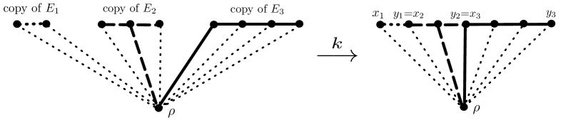
Figure 4: illustration of the map $k$

We endow the edges $e^{\prime}\in E^{\prime}$ with weights $W_{e^{\prime}}^{\prime}\geq 0$ as follows. For any edge $\{i,j\}\in E_{l}$ with $1\leq l\leq n$ and $\rho\notin\{i,j\}$, the corresponding edge $\{i^{l},j^{l}\}$ inherits its weight: $W_{i^{l}j^{l}}^{\prime}=W_{ij}$. Observe that a vertex $i\in\Lambda^{\prime}$ can be incident to edges in several $E_{l}$’s. For pinning edges $\{i,\rho\}$, we split the weight $W_{i\rho}$ as follows. In the case $\{i,\rho\}\in E_{l}$ for some $l$, we set $W_{i^{k}\rho}^{\prime}=(W_{i\rho}-\varepsilon)\delta_{kl}+\varepsilon/|\{l^{\prime}:i\in\Lambda_{E_{l^{\prime}}}\}|$, $1\leq k\leq n$; the index $l$ is unique since the $E_{l}$ are pairwise disjoint. In the case $\{i,\rho\}\notin E_{l}$ for all $l$, we set $W_{i^{k}\rho}^{\prime}=W_{i\rho}/|\{l:i\in\Lambda_{E_{l}}\}|$ for all $k$. Note that $\sum_{k=1}^{n}W_{i^{k}\rho}^{\prime}=W_{i\rho}$ and $W_{i^{k}\rho}^{\prime}\geq{\varepsilon}/n>0$ for all $k$ since $W_{i\rho}\geq{\varepsilon}$. For all other edges $e\in E^{\prime}$, we set $W_{e^{\prime}}^{\prime}=0$. For $1\leq l\leq n$, we set $e_{l}^{\prime}=\{x_{l}^{l},y_{l}^{l}\}\in E^{\prime}$ and $m_{e_{l}^{\prime}}^{\prime}=m_{e_{l}}$, but $m_{e^{\prime}}^{\prime}=0$ for all other edges $e^{\prime}\in E^{\prime}$. Then, Lemmas 5.7 and 5.9 and Remark 5.10 are applicable. In particular, on $U$ the bound $m_{e_{l}}\mathcal{R}^{G_{l}}(c,x_{l}\leftrightarrow y_{l})\leq 1-\theta$ and Remark 5.10 imply $m_{e_{l}}({\mathcal{G}}_{l})_{e_{l},e_{l}}\leq 1-\theta$ and then, by Lemma 5.9(b), $\sqrt{M_{l}}{\mathcal{G}}_{l}\sqrt{M_{l}}\leq(1-\theta)\operatorname{Id}$ for all $l$. As a consequence, by Lemma 5.9(a), $\sqrt{M^{\prime}}{\mathcal{G}}^{\prime}\sqrt{M^{\prime}}\leq(1-\theta)\operatorname{Id}$, which implies $\sqrt{M}{\mathcal{G}}\sqrt{M}\leq(1-\theta)\operatorname{Id}$ by Lemma 5.7. Note that this estimate is uniform in $\varepsilon>0$. Thus, by Lemma 5.5, Assumption 5.3 is satisfied, also in the limit $\varepsilon\to 0$. Combining formulas (5.42), (5.58), (5.59), and (5.62), we obtain

$$\det(\operatorname{Id}-M{\mathcal{G}}(u,s))\geq \det(\operatorname{Id}-M^{\prime}{\mathcal{G}}^{\prime}(u^{\prime},s^{\prime}))=\prod_{l=1}^{n}\det(\operatorname{Id}-M_{l}{\mathcal{G}}_{l})$$

$$= \prod_{l=1}^{n}(1-m_{e_{l}}({\mathcal{G}}_{l})_{e_{l},e_{l}})\geq\prod_{l=1}^{n}(1-m_{e_{l}}\mathcal{R}^{G_{l}}(c,x_{l}\leftrightarrow y_{l})).$$ (5.66)

Rayleigh’s monotonicity principle and its consequence (5.62) allow us to conclude.   

6 Bounding the environment – one-dimensional model

In this section, we will prove Theorem 4.2. We consider Model 4.1 with $\alpha>3$, possibly extended by additional non-nearest neighbor edges $e$ with weights $W_{e}\geq 0$. Throughout this section, $N$ is fixed and hence, we drop the dependence on $N$ in the notation. The important point is that the final estimates are uniform in $N$.

Recall that $e=\{x_{e},y_{e}\}$ and $x_{e}<y_{e}$ for $e\in E_{N}$. We take a sequence of cutoff parameters $\delta_{l}$, $l\in{\mathbb{N}}$ and associate the $\delta_{l}$ to nearest-neighbor edges on ${\mathbb{N}}$ by setting $\delta_{\{l-1,l\}}:=\delta_{l}$ for $l\geq 2$. Remember that we defined $\chi_{ij}=\chi_{e}=1_{(-\infty,1+\delta_{e})}$ for $e=\{i,j\}$. For $i<j$, we set

$$\overline{\chi}_{ij}:=\prod_{l=i+1}^{j}\chi_{l-1,l}(B_{l-1,l}).$$ (6.1)

Lemma 6.1

Let $E^{\prime},E^{\prime\prime}\subseteq E_{N}$ be disjoint subsets of $E_{N}$, where every $e\in E^{\prime}$ is a nearest neighbor edge: $y_{e}-x_{e}=1$, and for any two different $e,\tilde{e}\in E^{\prime}\cup E^{\prime\prime}$ the open intervals $(x_{e},y_{e})$ and $(x_{\tilde{e}},y_{\tilde{e}})$ are disjoint. Assume that $\sum_{l=1}^{\infty}\sqrt{\delta_{l}}<\infty$ and set $C_{\delta}=e^{\sqrt{2}\sum_{l=1}^{\infty}\sqrt{\delta_{l}}}$, which is uniform in $N$. Then, for all exponents $m_{e}$ satisfying $0\leq m_{e}<W_{e}$ for $e\in E^{\prime}$ and $0\leq m_{e}<\left(C_{\delta}\sum_{i=x_{e}+1}^{y_{e}}\frac{1}{W_{i-1,i}}\right)^{-1}$ for $e\in E^{\prime\prime}$, we have

$${\mathbb{E}}_{W,h}^{\Lambda_{N}}\left[\prod_{e\in E^{\prime}}B_{e}^{m_{e}}\cdot\prod_{e\in E^{\prime\prime}}(B_{e}^{m_{e}}\overline{\chi}_{e})\right]\leq\prod_{e\in E^{\prime}}\frac{1}{1-\frac{m_{e}}{W_{e}}}\prod_{e\in E^{\prime\prime}}\frac{1}{1-C_{\delta}m_{e}\sum_{i=x_{e}+1}^{y_{e}}\frac{1}{W_{i-1,i}}}.$$ (6.2)

Proof. We will show that Assumption 5.3 is satisfied and on the support of $\prod_{e\in E^{\prime\prime}}\overline{\chi}_{e}$, we have

$$\det(\operatorname{Id}-M{\mathcal{G}})\geq\prod_{e\in E^{\prime}}\left(1-\frac{m_{e}}{W_{e}}\right)\prod_{e\in E^{\prime\prime}}\left(1-C_{\delta}m_{e}\sum_{i=x_{e}+1}^{y_{e}}\frac{1}{W_{i-1,i}}\right).$$ (6.3)

It suffices to prove this in the case $W_{ij}=0$ for all edges $\{i,j\}$ with $|i-j|\geq 2$. The general case follows from Lemma 5.6. Using (6.3) and Lemma 5.4, we argue

$${\mathbb{E}}_{W,h}^{\Lambda_{N}} \left[\prod_{e\in E^{\prime}}B_{e}^{m_{e}}\cdot\prod_{e\in E^{\prime\prime}}(B_{e}^{m_{e}}\overline{\chi}_{e})\right]={\mathbb{E}}_{W,h}^{\Lambda_{N}}\left[\prod_{e\in E^{\prime}}B_{e}^{m_{e}}\cdot\prod_{e\in E^{\prime\prime}}(B_{e}^{m_{e}}\overline{\chi}_{e})\frac{\det(\operatorname{Id}-M{\mathcal{G}})}{\det(\operatorname{Id}-M{\mathcal{G}})}\right]$$

$$\leq \frac{{\mathbb{E}}_{W,h}^{\Lambda_{N}}\left[\prod_{e\in E^{\prime}}B_{e}^{m_{e}}\cdot\prod_{e\in E^{\prime\prime}}(B_{e}^{m_{e}}\overline{\chi}_{e})\det(\operatorname{Id}-M{\mathcal{G}})\right]}{\prod_{e\in E^{\prime}}\left(1-\frac{m_{e}}{W_{e}}\right)\prod_{e\in E^{\prime\prime}}\left(1-C_{\delta}m_{e}\sum_{i=x_{e}+1}^{y_{e}}\frac{1}{W_{i-1,i}}\right)}$$

$$\leq \prod_{e\in E^{\prime}}\frac{1}{1-\frac{m_{e}}{W_{e}}}\prod_{e\in E^{\prime\prime}}\frac{1}{1-C_{\delta}m_{e}\sum_{i=x_{e}+1}^{y_{e}}\frac{1}{W_{i-1,i}}},$$ (6.4)

which concludes the proof.

To prove (6.3), we apply Theorem 5.11 as follows. For $e\in E^{\prime}\cup E^{\prime\prime}$, we consider the pairwise disjoint sets of edges $E_{e}=\{\{\ i-1,i\}:\,x_{e}<i\leq y_{e}\}$ and the corresponding graphs $G_{e}=(\{x_{e},\ldots,y_{e}\},E_{e})$. In particular, $E_{e}=\{e\}$ for $e\in E^{\prime}$. We claim that

$$m_{e}\mathcal{R}^{G_{e}}(c,x_{e}\leftrightarrow y_{e})<1\quad\text{ for }e\in E^{\prime}\cup E^{\prime\prime}$$ (6.5)

holds on $U\subseteq\operatorname{supp}\prod_{e\in E^{\prime\prime}}\overline{\chi}_{e}$, cf. formula (5.22). Indeed, for the nearest-neighbor edges $e\in E^{\prime}$, we have

$$m_{e}\mathcal{R}^{G_{e}}(c,x_{e}\leftrightarrow y_{e})= \frac{m_{e}}{c_{e}}=\frac{m_{e}e^{u_{x_{e}}+u_{y_{e}}}}{W_{e}e^{u_{x_{e}}+u_{y_{e}}}B_{e}}\leq\frac{m_{e}}{W_{e}}<1.$$ (6.6)

For edges $e\in E^{\prime\prime}$, we will show

$$m_{e}\mathcal{R}^{G_{e}}(c,x_{e}\leftrightarrow y_{e})\leq m_{e}C_{\delta}\sum_{i=x_{e}+1}^{y_{e}}\frac{1}{W_{i-1,i}}<1.$$ (6.7)

The inequalities “$<1$” in (6.6) and (6.7) follow from the assumptions on $m_{e}$. Therefore, by Theorem 5.11, Assumption 5.3 is valid and we have

$$\det(\operatorname{Id}-M{\mathcal{G}})\geq\prod_{e\in E^{\prime}\cup E^{\prime\prime}}(1-m_{e}\mathcal{R}^{G_{e}}(c,x_{e}\leftrightarrow y_{e})).$$ (6.8)

Inserting the bounds (6.6) and (6.7), we obtain (6.3).

Finally we prove (6.7). Consider an edge $e\in E^{\prime\prime}$. Using the definition (5.60) of the conductances $c_{e}$ and the series law for the resistances between $x_{e}$ and $y_{e}$, we obtain

$$\mathcal{R}^{G_{e}}(c,x_{e}\leftrightarrow y_{e}) =\sum_{i=x_{e}+1}^{y_{e}}\frac{1}{c_{i-1,i}}=\sum_{i=x_{e}+1}^{y_{e}}\frac{e^{u_{x_{e}}+u_{y_{e}}}}{W_{i-1,i}e^{u_{i-1}+u_{i}}B_{e}}$$

$$\leq\sum_{i=x_{e}+1}^{y_{e}}\frac{e^{u_{x_{e}}-u_{i-1}+u_{y_{e}}-u_{i}}}{W_{i-1,i}},$$ (6.9)

where we used $B_{e}\geq 1$. On the support of $\overline{\chi}_{e}$, one has for all $l\in\{x_{e}+1,\ldots,y_{e}\}$,

$$1+\delta_{l}>B_{l-1,l}\geq\cosh(u_{l-1}-u_{l})\geq 1+\frac{1}{2}(u_{l-1}-u_{l})^{2}$$ (6.10)

and hence $|u_{l-1}-u_{l}|\leq\sqrt{2\delta_{l}}$. For $i=x_{e}+1,\ldots,y_{e}$, we estimate

$$u_{x_{e}}-u_{i-1}+u_{y_{e}}-u_{i}\leq\sum_{\begin{subarray}{c}l=x_{e}+1\\ l\neq i\end{subarray}}^{y_{e}}|u_{l-1}-u_{l}|\leq\sqrt{2}\sum_{\begin{subarray}{c}l=x_{e}+1\\ l\neq i\end{subarray}}^{y_{e}}\sqrt{\delta_{l}}\leq\log C_{\delta}.$$ (6.11)

Inserting this in (6.9) concludes the proof of (6.7).   

Using Lemma 6.1, we prove now the bounds for the environment in the effective model.

Proof of Theorem 4.2. We start with a pointwise bound on each factor $B_{e}^{m_{e}}$ corresponding to an edge $e\in E^{\prime\prime}$. For this purpose, keeping $e$ fixed for the moment, we abbreviate $x=x_{e}$, $y=y_{e}\geq x_{e}+1$ and $m=m_{e}\geq 0$. We consider the partition of unity (cf. Fig. 5)

Figure 5: cut-off functions used in the partition of unity

$$1=\overline{\chi}_{xy}+(1-\overline{\chi}_{xy})=\overline{\chi}_{xy}+\sum_{j=x+1}^{y}\chi^{c}_{j-1,j}\overline{\chi}_{j,y}\text{ with }\chi^{c}_{j-1,j}:=1-\chi_{j-1,j}(B_{j-1,j}),$$ (6.12)

where the constants $\delta_{j}:=\delta_{\{j-1,j\}}$ appearing in the definition $\chi_{\{j-1,j\}}(B)=1_{\{B<1+\delta_{j}\}}$ will be specified later. This means that either all nearest-neighbor pairs between $x$ and $y$ are protected in the sense that the factor $\chi_{j-1,j}$ of the corresponding edge is present or there is a largest index $j$ for which the edge $\{j-1,j\}$ is unprotected. We estimate the $j$-th summand in the last sum, using

$$\chi_{\{j-1,j\}}^{c}=1_{\{B_{j-1,j}\geq 1+\delta_{j}\}}\leq\left(\frac{B_{j-1,j}}{1+\delta_{j}}\right)^{p_{j}}$$ (6.13)

where $p_{j}>0$ will be also chosen later. Inserting this bound and multiplying with $B_{e}^{m}=B_{xy}^{m}$ yields

$$B_{e}^{m}\leq B_{xy}^{m}\overline{\chi}_{xy}+\sum_{j=x+1}^{y}(1+\delta_{j})^{-p_{j}}B_{xy}^{m}B_{j-1,j}^{p_{j}}\overline{\chi}_{j,y}.$$ (6.14)

We estimate $B_{xy}$ in the $j$-th summand as follows. By [DSZ10, Lemma 2 in Section 5.2], one has $B_{ij}\leq 2B_{ik}B_{kj}$ for all $i,j,k$. Given $j$ with $x+1\leq j\leq y$, this yields

$$B_{xy}\leq 2^{j-x}B_{jy}\prod_{i=x+1}^{j}B_{i-1,i},$$ (6.15)

with the convention $B_{yy}=1$. Inserting this in the $j$-th summand in (6.14), we obtain

$$B_{xy}^{m}\leq B_{xy}^{m}\overline{\chi}_{xy}+\sum_{j=x+1}^{y}\frac{2^{(j-x)m}}{(1+\delta_{j})^{p_{j}}}\left(\prod_{i=x+1}^{j-1}B_{i-1,i}^{m}\right)B_{j-1,j}^{m+p_{j}}B_{jy}^{m}\overline{\chi}_{jy}.$$ (6.16)

We now take the product of both sides of this inequality over $e=\{x_{e},y_{e}\}\in E^{\prime\prime}$, not suppressing the $e$-dependence in the notation anymore, and expand the product of sums on the r.h.s. in a sum of products. To keep the calculations readable, we introduce some abbreviations, locally for this proof. Let $X_{e,j}=\frac{2^{(j-x)m}}{(1+\delta_{j})^{p_{j}}}\left(\prod_{i=x+1}^{j-1}B_{i-1,i}^{m}\right)B_{j-1,j}^{m+p_{j}}B_{jy}^{m}\overline{\chi}_{jy}$, $j\in\{x_{e}+1,\ldots,y_{e}\}$, denote the summand on the r.h.s. of (6.16) indexed by $j$, and $X_{e,x_{e}}=B_{x_{e}y_{e}}^{m_{e}}\overline{\chi}_{x_{e}y_{e}}$ the first summand. We obtain

$$\prod_{e\in E^{\prime\prime}}B_{x_{e}y_{e}}^{m_{e}}\leq\prod_{e\in E^{\prime\prime}}\sum_{j=x_{e}}^{y_{e}}X_{e,j}=\sum_{(j_{e})_{e\in E^{\prime\prime}}\in\mathcal{I}}\prod_{e\in E^{\prime\prime}}X_{e,j_{e}}$$ (6.17)

with the cartesian product $\mathcal{I}=\prod_{e\in E^{\prime\prime}}\{x_{e},\ldots,y_{e}\}$. Therefore,

$${\mathbb{E}}\left[\prod_{e\in E^{\prime}}B_{x_{e}y_{e}}^{m_{e}}\cdot\prod_{e\in E^{\prime\prime}}B_{x_{e}y_{e}}^{m_{e}}\right]\leq\sum_{(j_{e})_{e\in E^{\prime\prime}}\in\mathcal{I}}{\mathbb{E}}\left[\prod_{e\in E^{\prime}}B_{x_{e}y_{e}}^{m_{e}}\cdot\prod_{e\in E^{\prime\prime}}X_{e,j_{e}}\right].$$ (6.18)

We will estimate the expectations in the sum using Lemma 6.1 showing that it is applicable for an appropriate choice of $\delta_{j}$ and $p_{j}$. We illustrate first the strategy in two special cases. In the special case that $E^{\prime}$ consists of a single edge $e=\{x_{e},y_{e}\}$ and $E^{\prime\prime}=\emptyset$, Lemma 6.1 gives

$${\mathbb{E}}\left[B_{x_{e}y_{e}}^{m_{e}}\right]\leq\frac{1}{1-\frac{m_{e}}{W_{e}}}=:Y_{e}$$ (6.19)

because $m_{e}<W_{e}$. Similarly, if $E^{\prime}=\emptyset$ and $E^{\prime\prime}$ consists of a single edge $e=\{x_{e},y_{e}\}$, Lemma 6.1 will give us

$${\mathbb{E}}\left[X_{e,x_{e}}\right]={\mathbb{E}}\left[B_{x_{e}y_{e}}^{m_{e}}\overline{\chi}_{x_{e}y_{e}}\right]\leq\frac{1}{1-C_{\delta}m_{e}\sum_{k=x_{e}+1}^{y_{e}}\frac{1}{W_{k-1,k}}}=:Y_{e,x_{e}}$$ (6.20)

and for $j\in\{x_{e}+1,\ldots,y_{e}\}$

$${\mathbb{E}} \left[X_{e,j}\right]=\frac{2^{(j-x_{e})m_{e}}}{(1+\delta_{j})^{p_{j}}}{\mathbb{E}}\left[\left(\prod_{i=x_{e}+1}^{j-1}B_{i-1,i}^{m_{e}}\right)B_{j-1,j}^{m_{e}+p_{j}}B_{jy_{e}}^{m_{e}}\overline{\chi}_{jy_{e}}\right]$$

$$\leq\frac{2^{(j-x_{e})m_{e}}}{(1+\delta_{j})^{p_{j}}}\prod_{i=x_{e}+1}^{j-1}\frac{1}{1-\frac{m_{e}}{W_{i-1,i}}}\cdot\frac{1}{1-\frac{m_{e}+p_{j}}{W_{j-1,j}}}\cdot\frac{1}{1-C_{\delta}m_{e}\sum_{k=j+1}^{y_{e}}\frac{1}{W_{k-1,k}}}=:Y_{e,j}.$$ (6.21)

In the general case, Lemma 6.1 will give

$${\mathbb{E}}\left[\prod_{e\in E^{\prime}}B_{x_{e}y_{e}}^{m_{e}}\cdot\prod_{e\in E^{\prime\prime}}X_{e,j_{e}}\right]\leq\prod_{e\in E^{\prime}}Y_{e}\cdot\prod_{e\in E^{\prime\prime}}Y_{e,j_{e}}$$ (6.22)

for all $(j_{e})_{e\in E^{\prime\prime}}\in\mathcal{I}$. Summing over $\mathcal{I}$ and recombining the sum over products to a product of sums, we obtain

$${\mathbb{E}}\left[\prod_{e\in E^{\prime}\cup E^{\prime\prime}}B_{x_{e}y_{e}}^{m_{e}}\right]\leq\sum_{(j_{e})_{e\in E^{\prime\prime}}\in\mathcal{I}}\prod_{e\in E^{\prime}}Y_{e}\cdot\prod_{e\in E^{\prime\prime}}Y_{e,j_{e}}=\prod_{e\in E^{\prime}}Y_{e}\cdot\prod_{e\in E^{\prime\prime}}\sum_{j=x_{e}}^{y_{e}}Y_{e,j}.$$ (6.23)

To check applicability of Lemma 6.1, we need $\delta_{j}$ and $p_{j}$ such that $\sum_{l=1}^{\infty}\sqrt{\delta_{l}}<\infty$ and all denominators in the $Y$-factors are strictly positive. For later use, some estimates will be sharper than needed at this point.

Recall the assumption on the weights $W_{j-1,j}\geq\overline{W}j^{\alpha}$ with $\alpha>3$. Let $\kappa\in(0,1]$ and $\gamma\geq 0$ with $\alpha-\gamma>3$ be given. We set $\delta_{j}:=j^{-(\alpha-\gamma-1)}$ for $j\in{\mathbb{N}}$. With this choice, we have

$$\sum_{l=1}^{\infty}\sqrt{\delta_{l}}=1+\sum_{l=2}^{\infty}l^{-\frac{\alpha-\gamma-1}{2}}\leq 1+\int_{1}^{\infty}t^{-\frac{\alpha-\gamma-1}{2}}\,dt=\frac{\alpha-\gamma-1}{\alpha-\gamma-3}<\infty.$$ (6.24)

We take now $c_{1},{c_{2}},{\overline{W}_{3}}$ as in (4.16) and (4.17) and $\overline{W}\geq{\overline{W}_{3}}$. For a given $e=\{x,y\}\in E^{\prime\prime}$, we consider $Y_{e,j}$ with $x\leq j\leq y$, suppressing the $e$-dependence again in the notation. We need to estimate $m/W_{i-1,i}$ for $x<i<y$, $(m+p_{j})/W_{j-1,j}$ for $x<j\leq y$, and $C_{\delta}m\sum_{k=j+1}^{y}\frac{1}{W_{k-1,k}}$ for $x\leq j\leq y$. Recall that $m_{x}=c_{1}\overline{W}x^{\gamma}={c_{2}}\overline{W}x^{\gamma}/\log 2$ and let $m\in[0,m_{x}]$. For all $i\geq x$, using $\gamma-\alpha<0$ and $c_{1}\leq(16\log 2)^{-1}\leq\frac{1}{4}$, we estimate

$$\frac{m}{W_{i-1,i}}\leq\frac{m_{x}}{\overline{W}i^{\alpha}}=c_{1}x^{\gamma}i^{-\alpha}\leq c_{1}x^{\gamma-\alpha}\leq c_{1}\leq\frac{1}{4}.$$ (6.25)

For $j\in{\mathbb{N}}$, we set $p_{j}:=4{c_{2}}\overline{W}j^{\alpha}$. For $x<j\leq y$, we obtain with ${c_{2}}\leq\frac{1}{16}$ the bound

$$\frac{m+p_{j}}{W_{j-1,j}}\leq\frac{1}{4}+\frac{p_{j}}{W_{j-1,j}}\leq\frac{1}{4}+\frac{p_{j}}{\overline{W}j^{\alpha}}=\frac{1}{4}+4{c_{2}}\leq\frac{1}{2}.$$ (6.26)

Finally, for $x\leq j\leq y$, we estimate, using $\alpha>3$,

$$\sum_{k=j+1}^{y}\frac{1}{W_{k-1,k}}\leq\sum_{k=j+1}^{y}\frac{1}{\overline{W}k^{\alpha}}\leq\int_{x}^{\infty}\frac{1}{\overline{W}t^{\alpha}}\,dt=\frac{x^{1-\alpha}}{\overline{W}(\alpha-1)}\leq\frac{x^{1-\alpha}}{2\overline{W}}.$$ (6.27)

Because of (6.24), the constant $C_{\delta}$ from Lemma 6.1 satisfies $1\leq C_{\delta}=e^{\sqrt{2}\sum_{l=1}^{\infty}\sqrt{\delta_{l}}}\leq e^{\sqrt{2}\frac{\alpha-\gamma-1}{\alpha-\gamma-3}}$. Hence, our choice of $c_{1}$ in (4.16) and (4.17) yields $c_{1}\leq\frac{2}{3}\kappa/C_{\delta}$. Together with (6.27), using $\gamma+1-\alpha<0$, it follows

$$C_{\delta}m\sum_{k=j+1}^{y}\frac{1}{W_{k-1,k}}\leq C_{\delta}m_{x}\frac{x^{1-\alpha}}{2\overline{W}}=\frac{C_{\delta}c_{1}x^{\gamma+1-\alpha}}{2}\leq\frac{C_{\delta}c_{1}}{2}\leq\frac{\kappa}{3}<1.$$ (6.28)

This shows that the assumptions of Lemma 6.1 needed above are fulfilled.

We now use the estimates above to bound the $Y$-variables defined in (6.20) and (6.21). Using $\kappa\in(0,1]$, one has $(1-t)^{-1}\leq 1+\kappa/2$ for all $t\in[0,\kappa/3]$. Consequently, (6.28) implies

$$\frac{1}{1-C_{\delta}m\sum_{k=j+1}^{y}\frac{1}{W_{k-1,k}}}\leq 1+\frac{\kappa}{2}\leq 2\text{ for }x\leq j\leq y.$$ (6.29)

In the case $j=x$, this yields

$$Y_{e,x}\leq 1+\frac{\kappa}{2}.$$ (6.30)

We consider now $x<j\leq y$. For $t\in[0,\frac{1}{2}]$, we have $(1-t)^{-1}\leq\min\{2,e^{2t}\}$. We apply this estimate to $t=\frac{m_{e}}{W_{i-1,i}}\leq\frac{1}{4}$, cf. (6.25), with $x<i<j$ and to $t=\frac{m+p_{j}}{W_{j-1,j}}\leq\frac{1}{2}$, cf. (6.26), to obtain, using (6.28) and $C_{\delta}\geq 1$,

$$\prod_{i=x+1}^{j-1}\!\!\frac{1}{1-\frac{m_{e}}{W_{i-1,i}}}\cdot\frac{1}{1-\frac{m_{e}+p_{j}}{W_{j-1,j}}}\leq 2\!\!\prod_{i=x+1}^{j-1}\!\!e^{2\frac{m}{W_{i-1,i}}}=2e^{2m\sum_{i=x+1}^{y-1}\frac{1}{W_{i-1,i}}}\leq 2e^{2\kappa/3}\leq 2e.$$ (6.31)

Substituting this and (6.29) in the definition (6.21) of $Y_{e,j}$, it follows, using in addition $\log(1+\delta_{j})\geq\delta_{j}/2$ since $\delta_{j}=j^{-(\alpha-\gamma-1)}\in[0,1]$,

$$Y_{e,j} \leq 4e\frac{2^{(j-x)m}}{(1+\delta_{j})^{p_{j}}}=4e\cdot e^{(j-x)m\log 2-p_{j}\log(1+\delta_{j})}\leq 4e\cdot e^{(j-x)m\log 2-\frac{1}{2}p_{j}\delta_{j}}$$

$$\leq 4e\cdot e^{jm_{x}\log 2-\frac{1}{2}p_{j}\delta_{j}}=4e\cdot e^{{c_{2}}\overline{W}x^{\gamma}j-2{c_{2}}\overline{W}j^{\gamma+1}}\leq 4e\cdot e^{-{c_{2}}\overline{W}j^{\gamma+1}}\leq 4e\cdot e^{-{c_{2}}\overline{W}j},$$ (6.32)

where we used $x\leq j$ and $\gamma\geq 0$ in the last two inequalities, respectively. Summing this bound over $j=x+1,\ldots,y$ and adding the bound (6.30) for $Y_{e,x}$ yields

$$\sum_{j=x}^{y}Y_{e,j}\leq 1+\frac{\kappa}{2}+4e\sum_{j=x+1}^{y}e^{-{c_{2}}\overline{W}j}\leq 1+\frac{\kappa}{2}+4e\frac{e^{-{c_{2}}\overline{W}(x+1)}}{1-e^{-{c_{2}}\overline{W}}}.$$ (6.33)

Using $\overline{W}\geq{\overline{W}_{3}}$ and our choice (4.16) of ${\overline{W}_{3}}$, we observe $e^{-{c_{2}}\overline{W}}\leq\sqrt{\kappa}/6$. Together with $x\geq 1$ and $\kappa\leq 1$ this yields

$$4e\frac{e^{-{c_{2}}\overline{W}(x+1)}}{1-e^{-{c_{2}}\overline{W}}}\leq 4e\frac{e^{-2{c_{2}}\overline{W}}}{1-e^{-{c_{2}}\overline{W}}}\leq 4e\frac{\left(\frac{\sqrt{\kappa}}{6}\right)^{2}}{1-\frac{1}{6}}=\frac{2e}{15}\kappa\leq\frac{\kappa}{2}.$$ (6.34)

We conclude $\sum_{j=x}^{y}Y_{e,j}\leq 1+\kappa$. Substituting this bound and the definition (6.19) of $Y_{e}$ in (6.23), we conclude

$${\mathbb{E}}\left[\prod_{e\in E^{\prime}\cup E^{\prime\prime}}B_{x_{e}y_{e}}^{m_{e}}\right]\leq\prod_{e\in E^{\prime}}Y_{e}\cdot\prod_{e\in E^{\prime\prime}}\sum_{j=x_{e}}^{y_{e}}Y_{e,j}\leq(1+\kappa)^{|E^{\prime\prime}|}\prod_{e\in E^{\prime}}\frac{1}{1-\frac{m_{e}}{W_{e}}}.$$ (6.35)

This proves claim (4.13). Claim (4.14) is a special case of bound (4.13), replacing $E^{\prime}$ and $E^{\prime\prime}$ by $\emptyset$ and $E^{\prime}\cup E^{\prime\prime}$, respectively. Alternatively, it follows from (4.13) and the bound $(1-\frac{m_{e}}{W_{e}})^{-1}\leq 1+\kappa$. Finally, (4.15) follows from (4.14) with $E^{\prime}=\emptyset$, $E^{\prime\prime}=\{e\}$, and the definition (4.2) of $B_{e}$.   

Proof of Lemma 4.3. In the proof of Theorem 4.2, we showed that ${\overline{W}_{3}}$, $c_{1}$, and ${c_{2}}$ can be chosen as in (4.16) and (4.17). Using $\overline{W}\geq{\overline{W}_{3}}$, $\gamma\geq 0$, $x\geq 1$, and $\kappa\leq 1$, we observe $m_{x}=c_{1}\overline{W}x^{\gamma}\geq c_{1}{\overline{W}_{3}}=-\log(\kappa/36)/(2\log 2)\geq\log_{2}6$. For $\overline{W}\geq{\overline{W}_{1}}=5{\overline{W}_{3}}/\log_{2}6$, one has $m_{x}\geq 5$. For $\kappa=1$, we obtain ${\overline{W}_{3}}=\log 6/{c_{2}}$, which yields the expressions in (4.19).   

7 Bounding the environment – hierarchical model

Proof of Theorem 3.3. By uniform pinning and the symmetry of the weights induced by the hierarchical structure, the distribution of $u_{i}$ is the same for all $i\in\Lambda_{N}$. Therefore, it is enough to prove (3.10) for the vertex $i_{1}:=0^{N}:=(0,\ldots,0)$. Corollary 2.3 of [DMR22] tells us that the distribution of $e^{u_{i_{1}}}$ in this model coincides with the distribution of $e^{u_{i_{1}}}$ in the effective $H^{2|2}$ model on the complete graph with vertex set $A=\{j,i_{1},\ldots,i_{N}\}\subseteq{\mathcal{T}}$, where $j:=(1,0^{N-1})=(1,0,\ldots,0)\in\{0,1\}^{N}$ and $i_{l}:=(1,0^{N-l})\in\{0,1\}^{N-l+1}$ for $2\leq l\leq N$. This is an antichain in the language of Section 2.3 of [DMR22] (cf. Figure 6).

Figure 6: the maximal antichain $A$

Weights and pinning are given in [DMR22, (2.13) and (2.14)], in particular, $W_{i_{l-1},i_{l}}=2^{(l-2)+(l-1)}w^{H}(l)=2^{2l-3}w^{H}(l)$, $h_{i_{l}}:=2^{l-1}h^{H}$, $2\leq l\leq N$, $h_{i_{1}}:=h^{H}$. Here, $2^{l-1}$ equals the number of leaves in ${\mathcal{T}}$ above the vertex $i_{l}=(1,0^{N-l})$. Corollary 2.3 of [DMR22] yields

$${\mathbb{E}}_{W^{H},h^{H}}^{\Lambda_{N}}[(\cosh u_{i_{1}})^{m}]={\mathbb{E}}_{W,h}^{A}[(\cosh u_{i_{1}})^{m}]={\mathbb{E}}_{W,h}^{A}[(\cosh(u_{i_{1}}-u_{\rho}))^{m}],$$ (7.1)

where in the last step we used $u_{\rho}=0$. We regard the pinning point $\rho$ as an additional vertex at the end of the antichain $j,i_{1},\ldots,i_{N}$, writing $i_{N+1}:=\rho$. Note that by assumption (3.9), one has $W_{i_{l-1}i_{l}}=2^{2l-3}w^{H}(l)\geq\overline{W}l^{\alpha}$ for $l\in\{2,\ldots,N\}$ and $W_{i_{N},i_{N+1}}=h_{i_{N}}=2^{N-1}h^{H}\geq\overline{W}(N+1)^{\alpha}$. Hence, we can apply the bound (4.15) in Theorem 4.2 for $x=i_{1}$, $y=i_{N+1}$, and case P2 which gives claim (3.10). The step from (3.10) to (3.11) is the same as the step from (1.8) to (1.9) in the long-range model; see its proof (3.24).   

Remark

We could get rid of the factor $2^{m}$ in (3.11) by connecting the vertices $i$ and $j$ by an antichain going twice over all levels below the least common ancestor in the binary tree. This antichain is described in Remark 4.2 and visualized in Figure 4.3 in [DMR22]. As a result, we obtain a one-dimensional effective model with nearest-neighbor weights that increase up to the middle and decrease afterwards. The strategy of the proof of Theorem 3.3 can be adapted to this case.

Acknowledgements: This work was supported by the DFG priority program SPP 2265 Random Geometric Systems. We are grateful to Malek Abdesselam for suggesting to compare the hierarchical model with the long-range model on ${\mathbb{Z}}^{d}$. We also thank Christophe Sabot, Pierre Tarrès, and Xiaolin Zeng for useful discussions.

References

- [ACK14] O. Angel, N. Crawford, and G. Kozma. Localization for linearly edge reinforced random walks. Duke Math. J., 163(5):889–921, 2014.
- [Bäu22] J. Bäumler. Recurrence and transience of symmetrice random walks with long range jumps. preprint, arXiv:2209.09901, 2022.
- [BH21] R. Bauerschmidt and T. Helmuth. Spin systems with hyperbolic symmetry: a survey. Proceedings of the ICM 2022, arXiv:2109.02566, 2021.
- [CFG09] P. Caputo, A. Faggionato, and A. Gaudillière. Recurrence and transience for long range reversible random walks on a random point process. Electron. J. Probab., 14:no. 90, 2580–2616, 2009.
- [DMR22] M. Disertori, F. Merkl, and S.W.W. Rolles. The non-linear supersymmetric hyperbolic sigma model on a complete graph with hierarchical interactions. ALEA Lat. Am. J. Probab. Math. Stat., 19(2):1629–1648, 2022.
- [DSZ10] M. Disertori, T. Spencer, and M.R. Zirnbauer. Quasi-diffusion in a 3D supersymmetric hyperbolic sigma model. Comm. Math. Phys., 300(2):435–486, 2010.
- [DV02] B. Davis and S. Volkov. Continuous time vertex-reinforced jump processes. Probab. Theory Related Fields, 123(2):281–300, 2002.
- [DV04] B. Davis and S. Volkov. Vertex-reinforced jump processes on trees and finite graphs. Probab. Theory Related Fields, 128(1):42–62, 2004.
- [LP16] R. Lyons and Y. Peres. Probability on trees and networks, volume 42 of Cambridge Series in Statistical and Probabilistic Mathematics. Cambridge University Press, New York, 2016.
- [PA22] R. Poudevigne-Auboiron. Monotonicity and phase transition for the VRJP and the ERRW. J. Eur. Math. Soc., 2022.
- [Sab21] C. Sabot. Polynomial localization of the 2D-vertex reinforced jump process. Electron. Commun. Probab., 26:Paper No. 1, 9, 2021.
- [ST15] C. Sabot and P. Tarrès. Edge-reinforced random walk, vertex-reinforced jump process and the supersymmetric hyperbolic sigma model. J. Eur. Math. Soc. (JEMS), 17(9):2353–2378, 2015.
- [Swa20] A. Swan. Superprobability on graphs (PhD thesis), 2020.
- [SZ19] C. Sabot and X. Zeng. A random Schrödinger operator associated with the vertex reinforced jump process on infinite graphs. J. Amer. Math. Soc., 32(2):311–349, 2019.
- [Zir91] M.R. Zirnbauer. Fourier analysis on a hyperbolic supermanifold with constant curvature. Comm. Math. Phys., 141(3):503–522, 1991.