Abstract

The Ablowitz-Ladik (AL) equations are distinguished integrable discretizations of the focusing and defocusing nonlinear Schrödinger (NLS) equations. In a previous paper we have studied the effect of the modulation instability of the homogeneous background solution of the AL equations in the periodic setting, showing in particular that both models exhibit instability properties, and studying, in terms of elementary functions, how a generic periodic perturbation of the unstable background evolves into a recurrence of anomalous waves (AWs). Using the finite gap method, in this paper we extend the recently developed perturbation theory for periodic NLS AWs to lattice equations, studying the effect of physically relevant perturbations of the $AL$ equations on the AW recurrence, like: linear loss, gain, and/or Hamiltonian corrections, in the simplest case of one unstable mode. We show that these small perturbations induce $O(1)$ effects on the periodic AW dynamics, generating three distinguished asymptotic patterns. Since dissipation and higher order Hamiltonian corrections can hardly be avoided in natural phenomena involving AWs, and since these perturbations induce $O(1)$ effects on the periodic AW dynamics, we expect that the asymptotic states described analytically in this paper will play a basic role in the theory of periodic AWs in natural phenomena described by discrete systems. The quantitative agreement between the analytic formulas of this paper and numerical experiments is excellent.

1 Introduction

The Ablowitz-Ladik (AL) equations [1, 2]:

$$\begin{array}[]{l}i\,\dot{u}_{n}+u_{n+1}+u_{n-1}-2u_{n}+\eta|u_{n}|^{2}\left(u_{n-1}+u_{n+1}\right)=0,\ \ \eta=\pm 1,\\ u_{n}=u(n,t)\in{\mathbb{C}},\ \ \dot{u}_{n}=\frac{du_{n}(t)}{dt},\ \ n\in{\mathbb{Z}},\ \ t\in{\mathbb{R}},\end{array}$$ (1)

are distinguished examples of integrable nonlinear differential-difference equations reducing, in the natural continuous limit

$$u_{n}(t)=ihv(\xi,\tau),\ \ hn=\xi,\ \ \tau=h^{2}t,\ \ h\to 0,$$ (2)

to the celebrated integrable [70] nonlinear Schrödinger (NLS) equations

$$\begin{array}[]{l}iv_{\tau}+v_{\xi\xi}+2\eta|v|^{2}v=0,\ \eta=\pm 1,\\ v(\xi,\tau)\in{\mathbb{C}},\ \ v_{\tau}=\frac{\partial v}{\partial\tau},\ \ v_{\xi\xi}=\frac{\partial^{2}v}{\partial{\xi}^{2}},\ \ \xi,\tau\in{\mathbb{R}},\end{array}$$ (3)

where $h$ is the lattice spacing. The two cases $\eta=\pm 1$ distinguish between the focusing ($\eta=1$) and defocusing ($\eta=-1$) NLS regimes.

The AL equations (1) characterize [34] the quantum correlation function of the XY-model of spins [39]. If $\eta=1$, it is relevant in the study of anharmonic lattices [61]; it is gauge equivalent to an integrable discretization of the Heisenberg spin chain [33], and appears in the description of a lossless nonlinear electric lattice ($\eta=1$) [42]. At last, if $\eta=1$, the AL hierarchy describes the integrable motions of a discrete curve on the sphere [14].

The well-known Lax pair of equations (1) reads [1, 2]

$$\begin{array}[]{l}\underline{\psi}_{n+1}(t,\lambda)=L_{n}(t,\lambda)\underline{\psi}_{n}(t,\lambda),\ \ \ \ {\dot{\underline{\psi}}_{n}}(t,\lambda)=A_{n}(t,\lambda)\underline{\psi}_{n}(t,\lambda),\\ L_{n}(t,\lambda)=\begin{pmatrix}\lambda&u_{n}(t)\\[5.69054pt] -\eta\overline{u}_{n}(t)&\frac{1}{\lambda}\end{pmatrix},\\ A_{n}(t,\lambda)=i\,\begin{pmatrix}\lambda^{2}-1+\eta u_{n}\overline{u}_{n-1}&\lambda u_{n}-\frac{u_{n-1}}{\lambda}\\[5.69054pt] \eta\frac{\overline{u}_{n}}{\lambda}-\eta\lambda\overline{u}_{n-1}&1-\frac{1}{\lambda^{2}}-\eta{u}_{n}\overline{u}_{n-1}\end{pmatrix},\end{array}$$ (4)

where $\bar{f}$ is the complex conjugate of $f$, and the matrices $L_{n}$ and $A_{n}$ of the Lax pair (4) possess the two symmetry

$$\begin{array}[]{l}L_{n}(\lambda)=P_{\eta}\,\overline{L_{n}\left(\frac{1}{\overline{\lambda}}\right)}P_{\eta}^{\dagger}=-\sigma_{3}\,L_{n}(-\lambda)\,\sigma_{3},\\ A_{n}(\lambda)=P_{\eta}\,\overline{A_{n}\left(\frac{1}{\lambda^{*}}\right)}P_{\eta}^{\dagger}=\sigma_{3}\,A_{n}(-\lambda)\,\sigma_{3},\end{array}$$ (5)

where

$$\sigma_{3}=\begin{pmatrix}1&0\\ 0&-1\end{pmatrix},\ \ \ \ P_{\eta}=\begin{pmatrix}0&-\eta\\ 1&0\end{pmatrix},$$ (6)

implying that, if $\underline{\psi}_{n}(\lambda,t)=({\psi_{1}}_{n}(\lambda,t),{\psi_{2}}_{n}(\lambda,t))^{T}$ is solution of (4), then

$$\check{\underline{\psi}}_{n}(\lambda,t)=\left(\begin{array}[]{c}-\eta\overline{{\psi_{2}}_{n}\left(\frac{1}{\overline{\lambda}},t)\right)}\\ \overline{{\psi_{1}}_{n}\left(\frac{1}{\overline{\lambda}},t)\right)}\end{array}\right),\ \ \hat{\underline{\psi}}_{n}(\lambda,t)=(-1)^{n}\left(\begin{array}[]{c}{\psi_{1}}_{n}(-\lambda,t)\\ -{\psi_{2}}_{n}(-\lambda,t)\end{array}\right)$$ (7)

are also a solution of (4). The Inverse Scattering Transform of the AL equations (1) for localized initial data was developed in [1, 2] (see also [4]), and for non zero boundary conditions and $\eta=1$ in [55]. The Finite Gap (FG) method [49, 15, 36, 29, 35] for periodic and quasi-periodic solutions was developed in [45].

Let $\Psi_{n}(t,\lambda)$ be a fundamental matrix solution of (4) for a periodic potential $u_{n}(t)$ of period $N$: $u_{n+N}(t)=u_{n}(t)$. Then it is well-known that the monodromy matrix

$$T(\lambda,t):=\Psi_{1+N}(t,\lambda)\Psi^{-1}_{1}(t,\lambda)=L_{N}(t,\lambda)L_{N-1}(t,\lambda)\dots L_{1}(t,\lambda)$$ (8)

satisfies the following properties.
i) $\det T=\prod\limits_{j=1}^{N}\left(1+\eta|u_{n}(t)|^{2}\right)$ is $t$- and $\lambda$-independent.
ii) $\mbox{tr}~{}T$ is a finite Laurent expansion in $\lambda$ with $t$-independent coefficients.

Unlike the NLS case, for which the homogeneous background solution is unstable under the perturbation of waves with sufficiently small wave numbers $\kappa$ in the focusing case $\eta=1$ [8, 7, 68, 69], and always stable in the defocusing case $\eta=-1$, the instability properties of the homogeneous background solution

$$a\exp(2\,i\,\eta\,|a|^{2}\,t),\ \ a\ \mbox{complex constant parameter},$$ (9)

of the AL equations (1) are much richer, and can be summarized as follows.

$$\begin{array}[]{ll}\mbox{If }\eta=1,&|\kappa|<\kappa_{a}:=\arccos\left(\frac{1-|a|^{2}}{1+|a|^{2}}\right),\ \forall|a|>0;\\ \mbox{if }\eta=-1,&|a|>1,\ \forall\kappa,\end{array}$$ (10)

where $\kappa_{a}$ is the smallest positive branch of $\arccos$ [5, 52, 12].

The set of exact AW solutions of the AL equations describing such nonlinear instability in the case of one and two unstable modes, are presented in [12]. In the case of one unstable mode they read

$${\mathcal{N}}(n,t;\kappa,X,T,\rho,\eta)=ae^{2i\eta|a|^{2}t+i\rho}\,\frac{\cosh\left[\sigma(\kappa)(t-T)+2i\eta\phi\right]+\eta G\cos[\kappa(n-X)]}{\,\cosh[\sigma(\kappa)(t-T)]-\eta G\cos[\kappa(n-X)]},$$ (11)

where

$$\cos\phi=\sqrt{1+\frac{\eta}{a^{2}}}\,\sin\left(\frac{\kappa}{2}\right),\ \ \ \ 0<\phi<\pi/2,$$ (12)

$$G=\frac{\sin\phi}{\cos\left(\frac{\kappa}{2}\right)},$$ (13)

$\kappa$ is the wave number,

$$\sigma(\kappa)=2\sqrt{(1+\eta|a|^{2})(1-\cos\kappa)\left[(1+\eta|a|^{2})\cos\kappa-(1-\eta|a|^{2})\right]}$$ (14)

is the growth rate of the linearized theory in the unstable cases (10), and $X$, $T$ and $\rho$ are arbitrary real parameters. Since $\phi$ is defined in terms of ($\kappa,a,\eta$) through (12), the growth rate $\sigma(\kappa)$ and the parameter $G$ can be expressed in terms of $(\kappa,a,\eta)$ or in terms of $(\phi,a,\eta$) in the following way:

$$\begin{array}[]{l}\sigma(\kappa)=2\sqrt{(1+\eta|a|^{2})(1-\cos\kappa)\left[(1+\eta|a|^{2})\cos\kappa-(1-\eta|a|^{2})\right]}\\ =2|a|^{2}\sin(2\phi),\\ G=\frac{\sin\theta}{\cos\left(\frac{\kappa}{2}\right)}=\sqrt{1-\frac{\eta}{|a|^{2}}\frac{1-\cos\kappa}{1+\cos\kappa}}=\frac{\sqrt{|a|^{2}+\eta}\sin\phi}{\sqrt{|a|^{2}\sin^{2}\phi+\eta}}.\end{array}$$ (15)

If $\eta=1$, (11) is the Narita solution [47] (see also [5]), discrete analogue of the well-known Akhmediev breather (AB) [6] solution of focusing NLS. If $\eta=-1$, (11) is the novel solution describing the MI present if $|a|>1$, $\forall\kappa\in{\mathbb{R}}$, unlike the NLS case, and this solution blows up at finite time [12]. In this respect we feel that the terminology “focusing” and “defocusing” NLS equations should not be exported to their AL discretizations, since not only the background solution of the AL equation reducing to the defocusing NLS is unstable under any monochromatic perturbation if $|a|>1$, but also such an instability leads generically to blow up at finite time [12]. Therefore we prefer to call the AL equations (1) for $\eta=\pm 1$ as $AL_{\pm}$ equations, instead of using the terminology “focusing and defocusing AL equations”, often present in the literature.

The Cauchy problem of the periodic AWs of the focusing NLS equation (3) has been recently solved in [19, 20], to leading order and in terms of elementary functions, for generic periodic initial perturbations of the unstable background:

$$\begin{array}[]{l}v(\xi,0)=a\left(1+\varepsilon w(\xi)\right),\ 0<\varepsilon\ll 1,\ w(\xi+L)=w(\xi),\\ w(\xi)=\sum_{j=1}^{\infty}(c_{j}e^{ik_{j}\xi}+c_{-j}e^{-ik_{j}\xi}),\ \ k_{j}=\frac{2\pi}{L}j,\end{array}$$ (16)

in the case of a finite number $N$ of unstable modes, using a suitable adaptation of the finite-gap (FG) method. In the simplest case of a single unstable mode ($N=1$), the above finite gap solution provides the analytic and quantitative description of an ideal Fermi-Pasta-Ulam-Tsingou (FPUT) recurrence [17] without thermalization, of periodic NLS AWs over the unstable background (9), described, to leading order, by the AB solution of focusing NLS for the arbitrary real parameters $\tilde{a},\rho,k,\tilde{X},\tilde{T}$, but with different parameters at each appearance [19]. See also [21] for an alternative and effective approach to the study of the AW recurrence in the case of a single unstable mode, based on matched asymptotic expansions; see [22] for a finite-gap model describing the numerical instabilities of the AB and [23] for the analytic study of the linear, nonlinear, and orbital instabilities of the AB within the NLS dynamics; see [24] for the analytic study of the phase resonances in the AW recurrence; see [56] and [12] for the analytic study of the FPUT AW recurrence in other NLS type models: respectively the PT-symmetric NLS equation [3] and the massive Thirring model [62, 44]. The AB, describing the nonlinear instability of a single mode, and its $N$-mode generalization were first derived respectively in [6] and [37]. The NLS recurrence of AWs in the periodic setting has been investigated in several numerical and real experiments, see, e.g., [65, 66, 28, 46, 54], and qualitatively studied in the past via a 3-wave approximation of NLS [32, 63].

In addition, a perturbation theory describing analytically how the FPUT recurrence of NLS AWs is modified by the presence of a small loss or gain has been recently introduced in [9], showing the these perturbations induce $O(1)$ effects on the periodic AW dynamics, and giving a theoretical explanation of previous interesting real and numerical experiments [28, 59]. The qualitative physical explanation of these analytic results is as follows. In the finite time interval when the AW appears, the non integrable loss/gain perturbation generates a small correction to the unperturbed solution, becoming an $O(1)$ correction when the next AW appears, due to MI. This theory has been applied in [10] to the complex Ginzburg-Landau [48] and Lugiato-Lefever [40] models, treated as perturbations of NLS; see also [11]. The case of a Hamiltonian perturbation was postponed to a subsequent paper, since in this case the leading order term in the main formula is identically zero in this case, and one should go to next order in the asymptotic expansion.

These NLS results suggest two interesting problems.
i) The construction of the analytic and quantitative description of the dynamics of periodic AWs on lattice models, using as prototype model the AL equations.
ii) The understanding of the effects of physically relevant perturbations, like loss, gain, and/or Hamiltonian corrections, on the AW dynamics on lattices.

In [12] we concentrated on the first problem. In particular, the periodic Cauchy problem of the AL equations (1), corresponding to a small initial periodic perturbation of the unstable background (9)

$$\begin{array}[]{l}u_{n+N}(t)=u_{n}(t),\ \ \forall n\in{\mathbb{Z}},\ \forall t\geq 0,\\ u_{n}(0)=a\left[1+{\epsilon}\left(\sum\limits_{j=1}^{p}\left(c_{j}e^{ik_{j}n}+c_{-j}e^{-ik_{j}n}\right)+c_{0}\right)\right],\ \ \ 0<{\epsilon}\ll 1,\end{array}$$ (17)

where

$$k_{j}=\frac{2\pi}{N}j,\ \ \ 1\leq j\leq p,\ \ \ p:=\left\{\begin{array}[]{ll}\frac{N}{2},&\mbox{if $N$ is even},\\ &\\ \frac{N-1}{2},&\mbox{if $N$ is odd},\end{array}\right.$$ (18)

has been solved, to leading order and in terms of elementary functions, in the case of one and two unstable modes for the $AL_{+}$ equation, using the matched asymptotics technique introduced in [21].

If $\eta=1$, the instability condition $|\kappa|<\kappa_{a}$ (10) implies that the first $M\leq p$ modes $\pm\kappa_{j},~{}1\leq j\leq M$ are unstable, where

$$M:=\left\lfloor{\frac{N\kappa_{a}}{2\pi}}\right\rfloor$$ (19)

and $\left\lfloor{x}\right\rfloor$ is the largest integer less or equal to $x\in{\mathbb{R}}$. If $M=1$ ($2\pi/\kappa_{a}<N<4\pi/\kappa_{a}$), the solution of the Cauchy problem (17) for $AL_{+}$ is described, to leading order, by the following expression, uniform in space-time, with $t\leq t^{(n)}+O(1)$:

$$u(x,t)=\sum\limits_{j=0}^{n}{\mathcal{N}}(x,t;\kappa_{1},x^{(j)},t^{(j)},\rho_{j},1)-ae^{2i|a|^{2}t}\frac{1-e^{4i\phi_{1}n}}{1-e^{4i\phi_{1}}}+O({\epsilon}).$$ (20)

where

$$\begin{array}[]{l}x^{(n)}=x^{(1)}+(n-1)\Delta x,\ x^{(1)}=\frac{\arg(\alpha_{1})+\pi/2}{\kappa_{1}},\ \mod N,\\ t^{(n)}=t^{(1)}+(n-1)\Delta t,\ \ t^{(1)}=\frac{1}{\sigma_{1}}\log\left(\frac{\sigma^{2}_{1}}{2|a|^{2}{\epsilon}|\alpha_{1}|\cos(\kappa_{1}/2)}\right),\\ \rho_{n}=2\phi_{1}+(n-1)4\phi_{1},\end{array}$$ (21)

$$\begin{array}[]{l}\Delta x=\frac{\arg(\alpha_{1}\beta_{1})}{\kappa_{1}},\mod N,\ \ \ \ \ \ \Delta t=\frac{1}{\sigma_{1}}\log\left(\frac{\sigma^{4}_{1}}{4|a|^{8}{\epsilon}^{2}|\alpha_{1}\beta_{1}|\cos^{2}(\kappa_{1}/2)}\right),\end{array}$$ (22)

and

$$\alpha_{1}:=\overline{c_{1}}e^{-i\phi_{1}}-c_{-1}e^{i\eta\phi_{1}},\ \ \beta_{1}=\overline{c_{-1}}e^{i\phi_{1}}-c_{1}e^{-i\phi_{1}}.$$ (23)

This is the analytic and quantitative description of the ideal Fermi-Pasta-Ulam-Tsingou (FPUT) recurrence of AWs of the $AL_{+}$ equation in term of the initial data through elementary functions. $x^{(1)}$ and $t^{(1)}$ are respectively the first appearance time and the position of the maximum of the absolute value of the AW; $\Delta x$ is the $x$-shift of the position of the maximum between two consecutive appearances, and $\Delta t$ is the time interval between two consecutive appearances (see Figure 1). The quantitative agreement between formulas (20)-(23) and numerical experiments is excellent, being even better than the expected theoretical estimate of one or more orders of magnitude [12]!

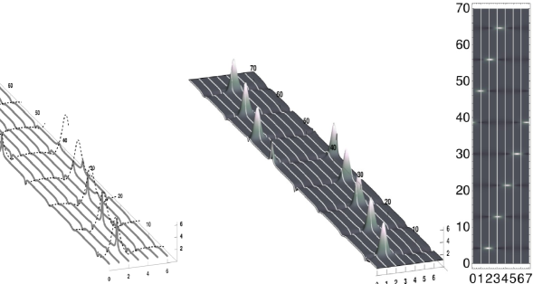
Figure 1: 3D plot of $|u_{n}(t)|$ coming from the numerical integration of the Cauchy problem of the AWs for the AL equation ($\eta=1$), in the case of a single unstable mode, using the 6th order Runge-Kutta method [57]; the short and long axes are respectively the lattice and time axes. Left: using dotted lines, we add to the figure the Narita solution $|{\mathcal{N}}|$ at the max of $|u_{n}(t)|$, coming from the theory (20)-(23). Centre: together with the numerical integration (white stripes), we plot the succession of Narita solitons as a continuous plot. Right, the density plot of the central graph. The initial condition $u_{n}(0)=a(1+\epsilon(c_{+}e^{ikn}+c_{-}e^{-ikn}))$, where $N=7$, $a=1.1$, $\epsilon=10^{-4}$, $c_{+}=0.53-i~{}0.86$, and $c_{-}=-0.26+i~{}0.22$. The sites are defined by lines parallel to the $t$-axis.

The same Cauchy problem for the $AL_{-}$ equation, in the case of one unstable mode, allows one to show analytically how a generic smooth initial perturbation of the background leads to a blow up at finite time described by the solution (11) with $\eta=-1$, whose free parameters are expressed in terms of the initial data via elementary functions [12].

We remark, from (21), that the maximum of the AW at the first appearance is located on a lattice point $x^{(1)}\in{\mathbb{Z}}$, if the initial data are such that $\frac{\arg\alpha_{1}}{\kappa_{1}}+\frac{N}{4}\in{\mathbb{Z}}$; if, in addition, $\Delta x\in{\mathbb{Z}}$, i.e., $\frac{\arg\beta_{1}}{\kappa_{1}}-\frac{N}{4}\in{\mathbb{Z}}$, the maxima of the FPUT recurrence are all located in the lattice points.

As in the NLS case, a very distinguished situation occurs when the initial data in (17) are such that $|c_{1}|=|c_{-1}|=:|c|$, corresponding to the case $\alpha_{1}\beta_{1}\in{\mathbb{R}}$:

$$\begin{array}[]{l}\alpha_{1}\beta_{1}=2|c|^{2}\left[\cos\gamma-\cos(2\phi_{1})\right]\in{\mathbb{R}},\ \ \ \ \gamma:=\arg(c_{1})+\arg(c_{-1}).\end{array}$$ (24)

Indeed, if $\alpha_{1}\beta_{1}>0$, then $\Delta x=0$ and the FPUT recurrence is periodic with period $\Delta t$. If $\alpha_{1}\beta_{1}<0$, then $\Delta x=N/2$ and the FPUT recurrence is periodic with period $2\Delta t$. Therefore, in terms of the initial data:

$$\begin{array}[]{l}|c_{1}|=|c_{-1}|,\ |\gamma|<2\phi_{1}\ \ \ \Leftrightarrow\ \ \ \alpha_{1}\beta_{1}>0,\\ |c_{1}|=|c_{-1}|,\ |\gamma|>2\phi_{1}\ \ \ \Leftrightarrow\ \ \ \alpha_{1}\beta_{1}<0.\end{array}$$ (25)

Particularly interesting subcases are $u_{n}(0)\in{\mathbb{R}}$ and $u_{n}(0)\in i{\mathbb{R}}$ [12].
a) If $u_{n}(0)\in{\mathbb{R}}$, then $|c_{1}|=|c_{-1}|,\ \gamma=0$, implying $\alpha_{1}\beta_{1}>0$, $\Delta x=0$, and a periodic FPUT recurrence with period $\Delta t$.
b) If $u_{n}(0)\in i{\mathbb{R}}$, then $|c_{1}|=|c_{-1}|,\ |\gamma|=\pi$, implying $\alpha_{1}\beta_{1}<0$, $\Delta x=N/2$, and a periodic FPUT recurrence with period $2\Delta t$.

Although the conditions (25) are not generic with respect to the AL dynamics, as we shall see in this paper, they describe the generic asymptotic state when the AL dynamics is perturbed by a small loss or gain, as in the NLS case. Since dissipation can hardly be avoided in all natural phenomena involving AWs, and since a small dissipation induces $O(1)$ effects on the periodic AW dynamics, generating the asymptotic states analytically described in this paper, we expect that these asymptotic states, together with their generalizations corresponding to more unstable modes, will play a basic role in the theory of periodic AWs in natural phenomena described by discrete systems.

In this paper we extend the NLS perturbation theory to lattices the $AL_{+}$ lattice, in order to show the order one effects of a small perturbation of the equation on the AW dynamics, and exemplify the theory on three basic examples: a linear loss, a linear gain, and a quintic Hamiltonian perturbation.

The paper is organized as follows. In §2 we construct the system of gaps corresponding to the background solution (9) of the AL equations, and to a generic periodic perturbation of the background solution; in §3 we construct the AW perturbation theory in the simplest case of one unstable mode; in §4 we apply theis theory to three relevant examples: a linear loss, a linear gain, and a quintic hamiltonian perturbation, enabling one to study quantitatively the order one effects of these perturbations on the AL AW dynamics described by formulas (20)-(23). The interesting problem of studying the AW dynamics of the physically relevant discrete NLS equations

$$\begin{array}[]{l}i\,\dot{u}_{n}+u_{n+1}+u_{n-1}-2u_{n}+\eta|u_{n}|^{2}u_{n}=0,\ \ \eta=\pm 1,\end{array}$$ (26)

viewed as a Hamiltonian perturbation of the AL lattices, is postponed to a subsequent paper.

2 The main spectrum of the perturbed background

To define the main spectrum associated with the periodic AW Cauchy problem, we find it convenient to work in the gauge defined by

$$\underline{w}_{n}(\lambda,t)=\frac{1}{\prod\limits_{j=0}^{n-1}\sqrt{1+\eta|u_{j}|^{2}}}\underline{\psi}_{n}(\lambda,t),$$ (27)

corresponding to the Lax pair (see the Appendix of [45])

$$\begin{array}[]{l}\underline{w}_{n+1}(\lambda,t)=\tilde{L}_{n}(t)\underline{w}_{n}(\lambda,t),\ \ \dot{\underline{w}}_{n}(\lambda,t)=\tilde{A}_{n}(\lambda,t)\underline{w}_{n}(\lambda,t),\\ \tilde{L}_{n}=\frac{1}{\sqrt{1+\eta|u_{n}|^{2}}}L_{n},\ \ \ \Rightarrow\ \ \det\tilde{L}_{n}=1,\\ \tilde{A}_{n}=i\begin{pmatrix}\frac{1}{2}\left(\lambda-\frac{1}{\lambda}\right)^{2}+\frac{\eta}{2}\left(u_{n}\overline{u}_{n-1}+\overline{u_{n}}u_{n-1}\right)&\lambda u_{n}-\frac{u_{n-1}}{\lambda}\\[5.69054pt] -\lambda\eta\,\overline{u}_{n-1}+\eta\frac{\overline{u_{n}}}{\lambda}&-\frac{1}{2}\left(\lambda-\frac{1}{\lambda}\right)^{2}-\frac{\eta}{2}\left(u_{n}\overline{u}_{n-1}+\overline{u_{n}}u_{n-1}\right)\end{pmatrix}.\end{array}$$ (28)

The corresponding monodromy matrix $\tilde{T}$ is simply related to $T$:

$$\begin{array}[]{l}\tilde{T}(\lambda,t):=\tilde{L}_{N}(\lambda,t)\tilde{L}_{N-1}(\lambda,t)\dots\tilde{L}_{1}(\lambda,t)=\frac{1}{\sqrt{\det T}}T(\lambda,t);\end{array}$$ (29)

then

$$\det\tilde{T}=1,\ \ \ \ \ \mbox{tr}\tilde{T}=\frac{\mbox{tr}T}{\sqrt{\det T}}$$ (30)

are also $t$-independent.

The eigenvalues of $\tilde{T}$:

$$\chi_{\pm}=\frac{\mbox{tr}\tilde{T}(\lambda)}{2}\pm\sqrt{\left(\frac{\mbox{tr}\tilde{T}(\lambda)}{2}\right)^{2}-1}$$ (31)

and its eigenvectors live on a two-sheeted covering $\Gamma$ of the $\lambda$ plane, due to the square root in (31), and play a crucial role in the construction of the Bloch eigenvectors, defined by the equations

$$\begin{array}[]{l}\vec{w}^{B,\pm}_{n+1}(\gamma)=\tilde{L}_{n}(t)\vec{w}^{B,\pm}_{n}(\gamma),\\ \\ \vec{w}^{B,\pm}_{n+N}(\gamma)=\chi_{\pm}(\gamma)\vec{w}^{B,\pm}_{n}(\gamma),\ \ \gamma\in\Gamma,\end{array}$$ (32)

where the Floquet multipliers $\chi_{\pm}(\gamma)$ are just the eigenvalues of the monodromy matrix $\tilde{T}$. The main spectrum is defined by the condition

$$|\chi(\gamma)|=1\ \ \ \ \Leftrightarrow\ \ \ \ -2\leq\mbox{tr}\tilde{T}(\lambda)\leq 2,$$ (33)

and, generically, consists of disconnected curves (the bands) in the complex $\lambda$ plane. The end points of the main spectrum, corresponding to periodic and anti-periodic Bloch eigenvectors and characterized by the conditions

$$\chi(\gamma)=\pm 1\ \ \ \ \Leftrightarrow\ \ \ \ \mbox{tr}\tilde{T}=\pm 2,$$ (34)

are the branch points and the multiple points (arising from the coalescence of two or more branch points). These end points are gauge independent and, in the original gauge (4), they are characterized instead by the condition

$$\mbox{tr}T=\pm 2\sqrt{\det T}.$$ (35)

We remark that the symmetries (5) imply the relations

$$\mbox{tr}\tilde{T}(\lambda)=(-\eta)^{N}\mbox{tr}\tilde{T}(1/\overline{\lambda})=-\mbox{tr}\tilde{T}(-\lambda).$$ (36)

Consequently the main spectrum and its end points are invariant under the transformations $\lambda\to 1/\overline{\lambda}$ and $\lambda\to-\lambda$ (if $\lambda$ belongs to the main spectrum, also $1/\overline{\lambda},-\lambda,-1/\overline{\lambda}$ belong to the main spectrum). In particular, if $\lambda$ is a branch point or a multiple point, then also $1/\overline{\lambda},-\lambda,-1/\overline{\lambda}$ are rispectively branch points or multiple points.

2.1 The main spectrum of the background

.

For the background solution $u^{[0]}_{n}(t)=ae^{2i\eta|a|^{2}t}$ the above quantities are explicit. The n-periodic matrix fundamental solution of the Lax pair (28) reads:

$$W^{[0]}_{n}(t)=e^{i\left(\eta|a|^{2}t+\frac{\arg a}{2}\right)\sigma_{3}}\begin{pmatrix}e^{s(\lambda)\,\exp(i\eta\,\mu)\,t}e^{i\,\eta\,\mu\,n}&&e^{s(\lambda)\,\exp(-i\eta\mu)\,t}e^{-i\,\eta\,\mu\,n}\\ g_{+}(\lambda)\,e^{s(\lambda)\,\exp(i\,\eta\,\mu)\,t}\,e^{i\,\eta\,\mu\,n}&&g_{-}(\lambda)\,e^{s(\lambda)\,\exp(-i\,\eta\,\mu)\,t}e^{-i\,\eta\,\mu\,n}\end{pmatrix},$$ (37)

where $\lambda$ and $\mu$ satisfy the equation

$$\cos\mu=\frac{1}{2\sqrt{1+\eta|a|^{2}}}\left(\lambda+\lambda^{-1}\right),$$ (38)

and

$$\begin{array}[]{l}g_{\pm}(\lambda)=\frac{1}{|a|}\left(-\frac{1}{2}\left(\lambda-\frac{1}{\lambda}\right)\pm\sqrt{\frac{1}{4}\left(\lambda-\frac{1}{\lambda}\right)^{2}-\eta|a|^{2}}\right),\\ s(\lambda)=i\sqrt{1+\eta|a|^{2}}\left(\lambda-\frac{1}{\lambda}\right).\end{array}$$ (39)

From equations (38) and (12) it follows that

$$\begin{array}[]{l}\sin\phi=\frac{1}{2|a|\sqrt{\eta}}\left(\lambda-\frac{1}{\lambda}\right),\ \ \ \cos\phi=\frac{1}{|a|}\sqrt{|a|^{2}-\eta\left(\frac{\lambda-\lambda^{-1}}{2}\right)^{2}},\\ \sin\mu=\frac{\sqrt{\eta|a|^{2}-\left(\frac{\lambda-\lambda^{-1}}{2}\right)^{2}}}{\sqrt{1+\eta|a|^{2}}},\end{array}$$ (40)

implying

$$g_{\pm}(\lambda)=\pm\frac{i}{\sqrt{\eta}}\,e^{\pm i\phi},$$ (41)

and

$$\begin{array}[]{l}W^{[0]}_{n}(t)=e^{i\left(\eta|a|^{2}t+\frac{\arg a}{2}\right)\sigma_{3}}\begin{pmatrix}e^{i\,\eta\,\mu\,n}&&e^{-i\,\eta\,\mu\,n}\\ \frac{i}{\sqrt{\eta}}e^{i\,\eta\,\left(\mu\,n+\phi\right)}&&-\frac{i}{\sqrt{\eta}}e^{-i\,\eta\,\left(\mu\,n+\phi\right)}\end{pmatrix}e^{-\frac{\sigma}{2}t\sigma_{3}+i\nu\,t},\\ \nu=2|a|\sqrt{\eta+|a|^{2}}\sin\phi\cos\mu\,t.\end{array}$$ (42)

Then the monodromy matrix reads

$$\begin{array}[]{l}\tilde{T}^{[0]}(\lambda,t)=W^{[0]}_{N+1}(t)\left(W^{[0]}_{1}\right)^{-1}(t)=W^{[0]}_{N}(t)\left(W^{[0]}_{0}\right)^{-1}(t)\\ =\frac{1}{\cos\phi}\begin{pmatrix}\cos\left(\mu N-\phi\right)&\frac{1}{\sqrt{\eta}}\sin\left(\mu N\right)e^{i\left(2\eta|a|^{2}t+\arg a\right)}\\ -\sqrt{\eta}\sin\left(\mu N\right)e^{-i\left(2\eta|a|^{2}t+\arg a\right)}&\cos\left(\mu N+\phi\right)\end{pmatrix}\end{array}$$ (43)

and

$$\mbox{tr}\tilde{T}^{[0]}(\lambda)=2\cos(\mu N).$$ (44)

The definition (33) of the main spectrum implies that $\mu\in{\mathbb{R}}$ and, from (38):

$$\begin{array}[]{ll}\{\lambda\in{\mathbb{R}},\ 1/\lambda_{0}\leq|\lambda|\leq\lambda_{0}\}\cup\{\lambda\in{\mathbb{C}},\ |\lambda|=1\},&\mbox{if }\eta=1,\\ \{\lambda=e^{i\theta},\ \theta\in{\mathbb{R}},\ \pi-\theta_{m}\leq|\theta|\leq\theta_{m}\},&\mbox{if }\eta=-1,\ |a|<1,\\ \{\lambda=ip,\ p\in{\mathbb{R}},\ 1/p_{0}\leq p\leq p_{0}\},&\mbox{if }\eta=-1,\ |a|>1,\end{array}$$ (45)

where

$$\lambda_{0}=\sqrt{1+|a|^{2}}+|a|,\ \ \theta_{m}=\arccos\left(\sqrt{1-|a|^{2}}\right),\ \ p_{0}=\sqrt{|a|^{2}-1}+|a|.$$ (46)

The end points of the main spectrum, corresponding to $\mbox{tr}\tilde{T}^{[0]}=\pm 2$, are characterized by

$$\mu_{n}=\frac{\pi}{N}n,\ \ \ 0\leq n\leq N.$$ (47)

From (38), for a given $\mu_{n},\ 0\leq n\leq N$, we have two values $\lambda^{\pm}_{n}$ of $\lambda$, corresponding to the $2N+2$ end points

$$\lambda^{\pm}_{n}=\sqrt{1+\eta|a|^{2}}\cos\mu_{n}\pm\sqrt{(1+\eta|a|^{2})\cos^{2}\mu_{n}-1},\ \ 0\leq n\leq N,$$ (48)

with the following symmetries:

$$\lambda^{-}_{n}=1/\lambda^{+}_{n}=-\lambda^{+}_{N-n},\ \ 0\leq n\leq N.$$ (49)

Since

$$\begin{array}[]{l}\partial_{\lambda}\mbox{tr}\tilde{T}_{0}(\lambda)=\frac{N}{\sqrt{1+\eta|a|^{2}}}\frac{(1-\lambda^{-2})\sin(\mu N)}{\sin\mu},\\ \partial^{2}_{\lambda}\mbox{tr}\tilde{T}_{0}(\lambda)=\frac{N}{\sqrt{1+\eta|a|^{2}}}\left\{2\frac{\sin(\mu N)}{\lambda^{3}\sin\mu}+(1-\lambda^{-2})\left[N\frac{\cos(\mu N)}{\sin\mu}-\frac{\sin(\mu N)\cos\mu}{\sin^{2}(\mu)}\right]\right\},\end{array}$$ (50)

it follows that

$$\partial_{\lambda}\mbox{tr}\tilde{T}_{0}(\lambda)\Big{|}_{\lambda^{\pm}_{0}}\neq 0,\ \ \partial_{\lambda}\mbox{tr}\tilde{T}_{0}(\lambda)\Big{|}_{\lambda^{\pm}_{N}}\neq 0,$$ (51)

implying that the four points $\lambda^{\pm}_{0}$, $\lambda^{\pm}_{N}$, are branch points (indicated by the symbol “X” in Figure 2); it also follows that

$$\begin{array}[]{l}\partial_{\lambda}T_{0}(\lambda)\Big{|}_{\lambda^{\pm}_{n}}=0,\\ \partial^{2}_{\lambda}T_{0}(\lambda)\Big{|}_{\lambda^{\pm}_{n}}=\frac{N^{2}}{\sqrt{1+\eta|a|^{2}}}\frac{(-1)^{n}}{\sin\mu_{n}}(1-(\lambda^{\pm}_{n})^{2})\neq 0,\ \ \ n\neq 0,N,\end{array}$$ (52)

implying that the remaining end points are double points (the black points and those indicated by the symbol “+” in Figure 2).

We have the following picture depending on $\eta$ and $|a|$.
i) $\eta=1$. The symmetries (49) suggest the following numeration rule

$$\lambda_{n}:=\lambda^{+}_{n},\ \ \ 0\leq n\leq\left\lfloor{\frac{N}{2}}\right\rfloor,$$ (53)

where

$$\begin{array}[]{lll}\lambda_{n}>1,&\lambda_{n}>\lambda_{n+1},&0\leq n\leq M,\\ \lambda_{n}=e^{i\arg\lambda_{n}},&\arg\lambda_{n}<\arg\lambda_{n+1},&M+1\leq n\leq\left\lfloor{\frac{N}{2}}\right\rfloor,\end{array}$$ (54)

where M is the number of unstable modes, as in (19).

Then the remaining end points are the sets

$$\{1/\lambda_{n},\ 0\leq n\leq\left\lfloor{\frac{N}{2}}\right\rfloor\},\{-\lambda_{n},\ 0\leq n\leq\left\lfloor{\frac{N}{2}}\right\rfloor\},\{-1/\lambda_{n},\ 0\leq n\leq\left\lfloor{\frac{N}{2}}\right\rfloor\}.$$ (55)

If $N$ is even, $\lambda_{\left\lfloor{\frac{N}{2}}\right\rfloor}=\lambda_{\frac{N}{2}}=i$, and in this case the four points reduce to two, since $-\lambda_{\frac{N}{2}}=1/\lambda_{\frac{N}{2}}$.

We remark that the reality condition $(1+|a|^{2})\cos^{2}\mu_{n}>1$ for the end points in (48) is equivalent to the instability condition (10), with $\kappa_{n}=2\mu_{n}$, Therefore the real double points

$$\begin{array}[]{l}\{\lambda_{n},1/\lambda_{n},-\lambda_{n},-1/\lambda_{n},\ 1\leq n\leq n_{c}\},\end{array}$$ (56)

correspond to the unstable modes (the black points in Figure 2), while the remaining double points, located on the unit circle (the points indicated by “+”), correspond to the stable modes.

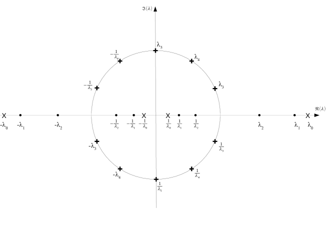
Figure 2: Spectrum in the complex $\lambda$ plane associated with the background solution of the AL equation, with periodicity N=10 and $a=1$. The double points of the spectrum associated with the unstable modes are the black points on the real axis, those associated with the stable modes, indicated by the symbol ”+”, are located on the unit circle. The four branch points are real and indicated by the symbol ”X”.

2.2 The main spectrum of a periodically perturbed background

Here we concentrate on the construction of the end points of the main spectrum associated with a periodic perturbation of the background. As we have seen, apart from the branch points $\lambda_{0},1/\lambda_{0},-\lambda_{0},-1/\lambda_{0}$, the remaining end points of the main spectrum of the background are double points. Therefore a generic periodic perturbation of the background will resolve such a degeneration in agreement with the following basic principles of perturbation theory for doubly degenerate eigenvalues.

Consider the eigenvalue equation for the unperturbed operator ${\mathcal{L}}_{0}$:

$${\mathcal{L}}_{0}|\psi>=\lambda|\psi>,$$ (57)

where $\lambda$ is a doubly degenerate eigenvalue corresponding to the two independent eigenfunctions $|f^{\pm}>$. Then the perturbed operator ${\mathcal{L}}={\mathcal{L}}_{0}+{\epsilon}{\mathcal{L}}_{1}$ resolves the degeneration in the following way:

$${\mathcal{L}}|\psi,\pm>=\left(\lambda+{\epsilon}\Delta^{\pm}\right)|\psi,\pm>,$$ (58)

where $\Delta^{\pm}$ are the eigenvalues of the $2\times 2$ matrix

$$V=\begin{pmatrix}<f^{+}|{\mathcal{L}}_{1}|f^{+}\;>&<f^{+}|{\mathcal{L}}_{1}|f^{-}>\\ <f^{-}|{\mathcal{L}}_{1}|f^{+}>&<f^{-}|{\mathcal{L}}_{1}|f^{-}>\end{pmatrix},$$ (59)

made of the matrix elements of the perturbation ${\mathcal{L}}_{1}$ with respect to the invariant subspace $\{|f^{-}>,|f^{+}>\}$ associated with the eigenvalue $\lambda$, $<f^{\pm}|$ are the corresponding elements of the dual basis such that

$$<f^{-}|f^{-}>=<f^{+}|f^{+}>=1,\ \ <f^{\mp}|f^{\pm}>=<f^{\mp}|f>=0,$$ (60)

and $|f>$ is any other element of the basis of eigenfunctions of ${\mathcal{L}}_{0}$.

To apply this result to our case, we first observe that the first equation in (28) (the spectral problem) can be written as the eigenvalue problem [45]

$${\mathcal{L}}_{n}\vec{w}_{n}=\lambda\vec{w}_{n},\ \ \ \ {\mathcal{L}}_{n}=\begin{pmatrix}\sqrt{1+\eta|u_{n}|^{2}}\textbf{E}&-u_{n}\\ -\eta\overline{u}_{n-1}&\sqrt{1+\eta|u_{n-1}|^{2}}\textbf{E}^{-1}\end{pmatrix},$$ (61)

where E is the forward lattice shift: $\textbf{E}f_{n}=f_{n+1}$. Let us specialize the previous formulas to the case $\eta=1$ and compute the effect of the initial monochromatic perturbation

$$u_{n}=a\left(1+{\epsilon}(c_{j}e^{ik_{j}n}+c_{-j}e^{-i\kappa_{j}n})\right)$$ (62)

on the spectrum discussed in the previous section.

Then ${\mathcal{L}}={\mathcal{L}}_{0}+{\epsilon}{\mathcal{L}}_{1}+O({\epsilon}^{2})$, where

$${\mathcal{L}}_{0}=\begin{pmatrix}\sqrt{1+|a|^{2}}\textbf{E}&-a\\[2.84526pt] -\bar{a}&\sqrt{1+|a|^{2}}\textbf{E}^{-1}\end{pmatrix},$$ (63)

$${\mathcal{L}}_{1}=\begin{pmatrix}\frac{|a|^{2}}{2\sqrt{1+|a|^{2}}}\left[(c_{j}+\overline{c_{j}})e^{2i\mu_{j}n}+(c_{-j}+\overline{c_{j}})e^{-2i\mu_{j}n}\right]\textbf{E}&-a\left(c_{j}e^{2i\mu_{j}n}+c_{-j}e^{-2i\mu_{j}n}\right)\\[2.84526pt] -\overline{a}(\overline{c_{j}}e^{-2i\mu_{j}(n-1)}+\overline{c_{-j}}e^{2i\mu_{j}(n-1)})&\frac{|a|^{2}}{2\sqrt{1+|a|^{2}}}\left[(c_{j}+\overline{c_{-j}})e^{2i\mu_{j}(n-1)}+(c_{-j}+\overline{c_{j}})e^{-2i\mu_{j}(n-1)}\right]\textbf{E}^{-1}\end{pmatrix}\;.$$

We use the following notation for the Bloch eigenfunctions (42) at $t=0$, in the generic double points $\lambda_{j},\ 1/\lambda_{j}$:

$$|\lambda_{j},\pm>=e^{i\frac{\arg a}{2}\sigma_{3}}\begin{pmatrix}1\\[8.53581pt] \pm ie^{\pm i\phi_{j}}\end{pmatrix}e^{\pm i\mu_{j}n}\;;\hskip 28.45274pt|\lambda^{-1}_{j},\pm>=e^{i\frac{\arg a}{2}\sigma_{3}}\begin{pmatrix}1\\[8.53581pt] \pm ie^{\mp i\phi_{j}}\end{pmatrix}e^{\pm i\mu_{j}n}\;;$$

where

$$\cos\phi_{j}=\frac{\sqrt{1+|a|^{2}}}{|a|}\,\sin\mu_{j},\ \ \ \ \kappa_{j}=2\mu_{j}.$$ (64)

Then

$$\begin{array}[]{l}V(\lambda_{j})=\begin{pmatrix}<+,\lambda_{j}|\,{\mathcal{L}}_{1}\,|\lambda_{j},+>&<+,\lambda_{j}|\,{\mathcal{L}}_{1}\,|\lambda_{j},->\\[8.53581pt] <-,\lambda_{j}|\,{\mathcal{L}}_{1}\,|\lambda_{j},+>&<-,\lambda_{j}|\,{\mathcal{L}}_{1}\,|\lambda_{j},->\end{pmatrix}\\ =\frac{|a|\lambda_{j}}{2\sqrt{1+|a|^{2}}\sin\phi_{j}}\begin{pmatrix}0&\beta_{j}e^{-i\mu_{j}-i\phi_{j}}\\ \alpha_{j}e^{i\mu_{j}+i\phi_{j}}&0\end{pmatrix},\end{array}$$

its eigenvalues are $\Delta^{\pm}_{j}=\pm\frac{|a|}{2\sqrt{1+|a|^{2}}}\frac{\lambda_{j}\sqrt{\alpha_{j}\beta_{j}}}{\sin\phi_{j}}$, and the double point $\lambda_{j}$ splits into the two branch points

$$E^{\pm}(\lambda_{j})=\lambda_{j}\left(1\pm{\epsilon}\frac{|a|}{2\sqrt{1+|a|^{2}}}\frac{\sqrt{\alpha_{j}\beta_{j}}}{\sin\phi_{j}}+O({\epsilon}^{2})\right),$$ (65)

generating the gap

$$E^{+}(\lambda_{j})-E^{-}(\lambda_{j})=\frac{{\epsilon}|a|\lambda_{j}\sqrt{\alpha_{j}\beta_{j}}}{\sqrt{1+|a|^{2}}\sin\phi_{j}}.$$ (66)

Proceeding in a similar way, one constructs the matrices $V(\lambda^{-1}_{j})$, $V(-\lambda_{j})$,$V(-\lambda^{-1}_{j})$; for instance

$$\begin{split}V\left(\lambda^{-1}_{j}\right)=-\frac{|a|}{2\sqrt{1+|a|^{2}}\sin\phi_{j}\lambda_{j}}\begin{pmatrix}0&&e^{i\phi_{j}-i\mu_{j}}\,\tilde{\beta}_{j}\\[8.53581pt] e^{-i\phi_{j}+i\mu_{j}}\,\tilde{\alpha}_{j}&&0\end{pmatrix},\end{split}$$

where

$$\tilde{\alpha}_{j}=\overline{c_{j}}e^{i\phi_{j}}-c_{-j}e^{-i\phi_{j}};\hskip 28.45274pt\tilde{\beta}_{j}=\overline{c_{-j}}e^{-i\phi_{j}}-c_{j}e^{i\phi_{j}}.$$

Therefore the double point $\lambda^{-1}_{j}$ splits into the two branch points

$$E^{\pm}(\lambda^{-1}_{j})=\lambda^{-1}_{j}\left(1\mp\frac{{\epsilon}|a|}{2\sqrt{1+|a|^{2}}}\frac{\sqrt{\tilde{\alpha}_{j}\tilde{\beta}_{j}}}{\sin\phi_{j}}+O({\epsilon}^{2})\right).$$ (67)

If $\lambda_{j}\in{\mathbb{R}}$ (the corresponding mode is unstable), the splitting is generic: $\alpha_{j}\beta_{j}$ is an arbitrary complex parameter and the corresponding gap $E^{+}-E^{-}$ has an arbitrary inclination and length. In addition, since $\tilde{\alpha}_{j}\tilde{\beta}_{j}=\overline{\alpha_{j}\beta_{j}}$, the branch points associated with $\lambda_{j}$ and $\lambda^{-1}_{j}$ satisfy the symmetry relation

$$E^{\pm}(\lambda^{-1}_{j})=\frac{1}{\overline{E^{\pm}(\lambda_{j})}}.$$ (68)

If $\lambda_{j}$ is on the unit circle: $\lambda_{j}=e^{i\arg\lambda_{j}}$ (the corresponding mode is stable), then $\phi_{j}\in i{\mathbb{R}}$ and

$$\begin{array}[]{l}\cos\mu_{j}=\frac{\cos(\arg\lambda_{j})}{\sqrt{1+|a|^{2}}},\ \ \ \ \sin\phi_{j}=i\frac{\sin(\arg\lambda_{j})}{\sqrt{1+|a|^{2}}},\ \ \ \ \beta_{j}=-\overline{\alpha_{j}};\end{array}$$ (69)

therefore

$$E^{\pm}(\lambda_{j})=\lambda_{j}\left(1\pm\frac{{\epsilon}|a|}{2\sqrt{1+|a|^{2}}}\frac{|\alpha_{j}|}{\sin(\phi_{j})}+O({\epsilon}^{2})\right).$$ (70)

It follows that the corresponding branch points are on the line from the origin to $\lambda_{j}$ (the splitting is radial), and satisfy the relation (see Figure 3)

$$E^{-}(\lambda_{j})=\frac{1}{\overline{E^{+}(\lambda_{j})}}.$$ (71)

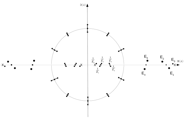
Figure 3: The effect of an initial generic periodic perturbation on the spectrum of Figure 2. The degenerate double points are now open gaps. The ones corresponding to the double points on the unit circle are radial; the ones corresponding to double points on the real axis have arbitrary inclination.

We finally remark that, since the product $\alpha_{1}\beta_{1}$ plays a basic role in the FPUT recurrence of AL AWs, appearing in the definitions (22) of $\Delta x$ and $\Delta t$, and since such a product appears also in the definition (66) of the gap $E^{+}(\lambda_{1})-E^{-}(\lambda_{1})$, it is possible to express $\Delta x$ and $\Delta t$ in terms of the gap, obtaining the spectral representation of the FPUT recurrence:

$$\begin{array}[]{l}\Delta x=\frac{2}{\kappa_{1}}\arg\left(E^{+}(\lambda_{1})-E^{-}(\lambda_{1})\right),\\ \Delta t=\frac{1}{\sigma_{1}}\log\left(\frac{\sigma_{1}^{4}\lambda_{1}^{2}}{4|a|^{6}(1+|a|^{2})\sin^{2}(\phi_{1})\cos^{2}(\kappa_{1}/2)|E^{+}(\lambda_{1})-E^{-}(\lambda_{1})|^{2}}\right).\end{array}$$ (72)

3 FPUT recurrence of AWs for the perturbed $AL_{+}$ equation

The main spectrum is a constant of motion with respect to the $AL_{+}$ time evolution. If one perturbs such evolution:

$$\dot{u}_{n}=i\,\left(u_{n+1}+u_{n-1}-2u_{n}+|u_{n}|^{2}\left(u_{n-1}+u_{n+1}\right)\right)+f[u_{n}],\ \ |f[u_{n}]|\ll 1,$$ (73)

or, in matrix form

$$\dot{L}_{n}=A_{n+1}L_{n}-L_{n}A_{n}+F[u_{n}],\ \ \ \ F[u_{n}]=\begin{pmatrix}0&f[u_{n}]\\ -\overline{f[u_{n}]}&0\end{pmatrix},$$ (74)

the main spectrum evolves in time generically in a non integrable fashion, and the theory of perturbations of integrable nonlinear evolution equations is the proper tool to have an analytic description of the effect of such a small perturbation on the dynamics under scrutiny.

From the variation of the monodromy matrix $T$ in (8):

$$\begin{array}[]{l}\delta T(\lambda,t)=\sum\limits_{n=1}^{N}L_{N}\dots L_{n+1}\left(\delta L_{n}\right)L_{n-1}\dots L_{1},\\ \delta L_{n}=\begin{pmatrix}0&\delta u_{n}\\ -\overline{\delta u_{n}}&0\end{pmatrix},\end{array}$$ (75)

it follows that the trace of such a variation can be expressed in terms of the so-called transition matrix

$$\hat{T}(n,m,\lambda,t):=\Psi_{n}(t,\lambda)\Psi^{-1}_{m}(t,\lambda)=L_{n-1}L_{n-2}\dots L_{m}$$ (76)

as follows

$$\begin{array}[]{l}\mbox{tr}\left(\delta T(\lambda,t)\right)=\sum\limits_{n=1}^{N}\mbox{tr}\left(L_{n-1}\dots L_{1}L_{N}\dots L_{n+1}\left(\delta L_{n}\right)\right)\\ =\sum\limits_{n=1}^{N}\mbox{tr}\left(L_{N+n-1}\dots L_{n+1}\left(\delta L_{n}\right)\right)=\sum\limits_{n=1}^{N}\mbox{tr}\left(\hat{T}(N+n,n+1,\lambda,t)\delta L_{n}\right),\end{array}$$ (77)

where we have used first the permutation properties of the trace and then the periodicity of $L_{n}$.

Equation (77) is valid for any variation; in our case $\delta u_{n}(t)=\dot{u}_{n}dt$, then $\delta T=\dot{T}dt$, $\delta L_{n}=\dot{L}_{n}dt$, and equation (77) becomes

$$\begin{array}[]{l}\mbox{tr}\left(\dot{T}(\lambda,t)\right)=\sum\limits_{n=1}^{N}\mbox{tr}\left(\hat{T}(n+N,n+1,\lambda,t)\dot{L}_{n}\right)\\ =\sum\limits_{n=1}^{N}\mbox{tr}\left(\hat{T}(n+N,n+1,\lambda,t)\left[A_{n+1}L_{n}-L_{n}A_{n}+F[u_{n}]\right]\right)\\ =\sum\limits_{n=1}^{N}\mbox{tr}\left(\hat{T}(n+N,n+1,\lambda,t)F[u_{n}]\right)=\sum\limits_{n=1}^{N}\mbox{tr}\left(\hat{T}(n+N,n,\lambda,t)L^{-1}_{n}F[u_{n}]\right),\end{array}$$ (78)

where we have used first the fact that the AL vector field $A_{n+1}L_{n}-L_{n}A_{n}$ is not responsible for the time evolution of $\mbox{tr}T$, and second the definitions (75) and (76) of $\delta L_{n}$ and of the transition matrix.

Recalling the relation (30) between the trace of T and that of $\tilde{T}$, we obtain the time derivative of $\mbox{tr}\tilde{T}$ in terms of the perturbation:

$$(\mbox{tr}\tilde{T})_{t}=\left(\frac{\mbox{tr}(T(\lambda,t))}{\sqrt{\det T(\lambda,t)}}\right)_{t}=\frac{\mbox{tr}\left(\sum\limits_{n=1}^{N}\left[2\hat{T}(n+N,n,\lambda,t)-\mbox{tr}T(\lambda,t)\right]L^{-1}_{n}F[u_{n}]\right)}{2\sqrt{\det T(t)}}.$$ (79)

Equation (79) describes in a rather implicit and nonlinear way the time evolution of the main spectrum, due to the nonintegrable perturbation $F[u_{n}]$. A crucial simplification arises from the observation that, in the AW recurrence, during the linear stages of MI, characterized by the background solution, $\mbox{tr}\tilde{T}$ is essentially constant (see Figures 4,7 below). Therefore the variation takes place in the finite intervals in which the AWs appear, described to leading order by the AW solution, and since the Narita solution is exponentially localized in time, one can replace the integral over the time interval of appearance by an integral over the real time axis.

In conclusion the variation of $\mbox{tr}\tilde{T}$ at each appearance of the AW is described by the following basic formula of the perturbation theory

$$\Delta\left(\mbox{tr}\tilde{T}(\lambda)\right)=\int\limits_{-\infty}^{\infty}\frac{\mbox{tr}\left(\sum\limits_{n=1}^{N}\left[2\hat{T}(n+N,n,\lambda,t)-\mbox{tr}T(\lambda,t)\right]L^{-1}_{n}F[u_{n}(t)]\right)}{2\sqrt{\det T(\lambda,t)}}dt,$$ (80)

where all the quantities inside the integral (the transition and monodromy matrices, $L_{n}$ and $u_{n}$) correspond to the AW solution (11). For instance (see the Appendix for details):

$$\begin{array}[]{l}\hat{T}(n+N,n;\lambda_{1})=\\ =\left(1+\,|a|^{2}\right)^{\frac{N}{2}}\left[-1+\frac{2N|a|\sqrt{1+|a|^{2}}\sin^{2}\phi\cos\frac{k}{2}\;g_{n}(t)}{\cos^{2}\phi\;H_{n}(t)}\begin{pmatrix}\overline{q_{1}(n)}\overline{q_{2}(n)}&-\overline{q_{2}(n)}\overline{q_{2}(n)}\\[5.69054pt] \overline{q_{1}(n)}\overline{q_{1}(n)}&-\overline{q_{1}(n)}\overline{q_{2}(n)}\end{pmatrix}\right]\;,\end{array}$$ (81)

where

$$\begin{array}[]{l}{q_{1}}_{n}=2\cos\left(\frac{\kappa(n-x_{1})+i\eta\sigma(t-t_{1})-\phi}{2}\right)e^{i\eta|a|^{2}t+i\frac{\arg a}{2}+i\nu t},\\ {q_{2}}_{n}=-2\sqrt{\eta}\sin\left(\frac{\kappa(n-x_{1})+i\eta\sigma(t-t_{1})+\phi}{2}\right)e^{-i\eta|a|^{2}t-i\frac{\arg a}{2}+i\nu t},\end{array}$$ (82)

and

$$g_{n}(t)=q_{1}(n)q_{1}(n)e^{-2i|a|^{2}t}+q_{2}(n)q_{2}(n)e^{2i|a|^{2}t}+2q_{1}(n)q_{2}(n)\sin\phi=4\cos^{2}\phi\;,$$ (83)

$$\begin{array}[]{l}H_{n}(t)=\left(\frac{|q_{1}(n)|^{2}}{\lambda_{1}}+\lambda_{1}|q_{2}(n)|^{2}\right)\left(\lambda_{1}|q_{1}(n)|^{2}+\frac{|q_{2}(n)|^{2}}{\lambda_{1}}\right)=\\ =16(1+|a|^{2})\left[\cos\frac{k}{2}\cosh(\sigma(t-t_{1}))-\cos\left(k\left(n-x_{1}\right)\right)\sin\phi\right]\left[\cos\frac{k}{2}\cosh(\sigma(t-t_{1}))-\cos\left(k\left(n-x_{1}-1\right)\right)\sin\phi\right].\end{array}$$ (84)

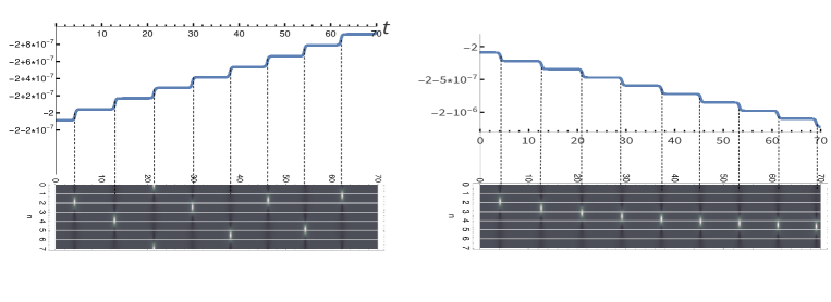
Figure 4: Dynamics of the real part $\Re\left(\frac{Tr(T)}{\sqrt{\det T}}\right)$ of $Tr(\tilde{T})$, in the presence of the small loss $\nu=10^{-8}$ or gain $\nu=-10^{-8}$. The variation corresponds to the AW appearance. The initial condition is: $u_{n}(0)=a(1+\epsilon(c_{+}e^{ik_{1}n}+c_{-}e^{-ik_{1}n}))$, with $a=1.1$, $\epsilon=10^{-4}$, $k_{1}=\frac{2\pi}{N}$, $N=7$, $c_{+}=0.53-i~{}0.86$ and $c_{-}=-0.26+i~{}0.22$.

On the other hand, reasoning as in [9], for $\lambda\sim\lambda_{1}$:

$$\mbox{tr}\tilde{T}(\lambda)\sim\frac{\mbox{tr}\;T(\lambda_{1})}{\sqrt{\det T}}+\left(\frac{N\sin\phi_{1}}{\lambda_{1}\cos\phi_{1}}\right)^{2}(\lambda-\lambda_{1})^{2}.$$ (85)

Evaluating this formula at $\lambda=E^{+}(\lambda_{1})$ and recalling that $E^{+}(\lambda_{1})-E^{-}(\lambda_{1})=2(E^{+}(\lambda_{1})-\nobreak\lambda_{1})$ and $\mbox{tr}\tilde{T}(E^{+}(\lambda_{1}))=-2$, we have

$$\begin{array}[]{l}\mbox{tr}\tilde{T}(\lambda_{1})=\frac{Tr\;T(\lambda_{1})}{\sqrt{\det T}}\sim-2-\left(\frac{N\sin\phi_{1}}{2\lambda_{1}\cos\phi_{1}}\right)^{2}(E^{+}(\lambda_{1})-E^{-}(\lambda_{1}))^{2},\end{array}$$ (86)

implying that

$$\Delta\left(\mbox{tr}\tilde{T}(\lambda_{1})\right)\sim-\left(\frac{N\sin\phi_{1}}{2\lambda_{1}\cos\phi_{1}}\right)^{2}\Delta(E^{+}(\lambda_{1})-E^{-}(\lambda_{1}))^{2}$$ (87)

Equations (80) and (87) complete the perturbation theory. In the following we apply it to three physically relevant perturbations, a linear loss, a linear gain, and a quintic Hamiltonian perturbation.

3.1 Linear loss or gain perturbations

If the perturbation is a linear loss or gain:

$$\begin{array}[]{l}f[u_{n}]=\nu u_{n},\ \ |\nu|\ll 1,\ \ \ \mbox{loss}:\ \nu<0;\ \ \ \mbox{gain}:\ \nu>0,\\ \Rightarrow\ \ \ F[u_{n}]=\nu U_{n}(t),\ \ \ \ U_{n}:=\begin{pmatrix}0&u_{n}\\ -\overline{u}_{n}&0\end{pmatrix},\end{array}$$ (88)

we can express the variation of $\mbox{tr}\tilde{T}$ after the $j^{th}$ appearance of the AW, through the analytic formula:

$$\begin{array}[]{l}\Delta_{j}(\mbox{tr}\tilde{T})=\Delta_{j}\left(\frac{Tr(T)}{\sqrt{\det T}}\right)=\frac{2N\sqrt{1+|a|^{2}}\sin^{2}\phi\cos\frac{k}{2}}{\cos^{2}\phi}\int_{-\infty}^{\infty}\sum_{n=1}^{N}\frac{g_{n}(t)h_{n}(t)}{H_{n}(t)(1+|u_{n}(t)|^{2})}dt\\ =-\nu\frac{2N|a|^{2}\sin^{2}\phi\cos\left(\frac{k}{2}\right)}{(1+|a|^{2})}I(\phi,x_{j}),\end{array}$$ (89)

where $g_{n}(t),H_{n}(t)$ are defined in (83),

$$\begin{split}&h_{n}(t)=\lambda_{1}\overline{u}_{n}\overline{q_{2}}^{2}+\frac{u_{n}}{\lambda_{1}}\overline{q_{1}}^{2}=\\ &=-4|a|\sqrt{1+|a|^{2}}\left(\cos\frac{k}{2}\cos(2\phi)+\cos\left(k\left(n-x_{j}\right)-i\sigma t\right)\sin\phi\right)\times\\ &\hskip 113.81102pt\times\frac{\left(\cos\frac{k}{2}\cosh(\sigma t)-\cos\left(k\left(n-x_{j}-1\right)\right)\sin\phi\right)}{\left(\cos\left(\frac{k}{2}\right)\cosh(\sigma(t-t_{1}))-\sin\phi\cos\left(k(n-x_{j})\right)\right)},\end{split}$$

and

$$I(\phi,x_{j})=\int_{-\infty}^{\infty}\left[\sum_{n=1}^{N}\frac{\cos\frac{\kappa}{2}\cos(2\phi)+\sin\phi\cos\left(\kappa_{1}\left(n-x_{j}\right)\right)\cosh\left(\sigma_{1}t\right)}{\left[\cos\frac{k}{2}\cosh(\sigma t)-\cos\left(k\left(n-x_{j}+1\right)\right)\sin\phi\right]\left[\cos\frac{k}{2}\cosh(\sigma t)-\cos\left(k\left(n-x_{j}-1\right)\right)\sin\phi\right]}\right]dt\;.$$

Note that $1+|u_{n}(t)|^{2}$ can be written as:

$$\begin{split}1+|u_{n}|^{2}=(1+|a|^{2})&\left[\cos\left(\frac{k}{2}\right)\cosh(\sigma(t-t_{1}))-\sin\phi\cos\left(k(n-x_{1}+1)\right)\right]\times\\[5.69054pt] &\times\frac{\left[\cos\left(\frac{k}{2}\right)\cosh(\sigma(t-t_{1}))-\sin\phi\cos\left(k(n-x_{1}-1)\right)\right]}{\left[\cos\left(\frac{k}{2}\right)\cosh(\sigma(t-t_{1}))-\sin\phi\cos\left(k(n-x_{1})\right)\right]^{2}}.\end{split}$$

Comparing equations (89) and (87) we infer that the effect of the j-th AW appearance is to modify the gap according to the formula:

$$\Delta_{j}(E^{+}(\lambda_{1})-E^{-}(\lambda_{1}))^{2}=\nu\frac{8|a|^{2}\lambda_{1}^{2}\cos^{2}\phi\cos\frac{\kappa_{1}}{2}}{N(1+|a|^{2})}\;I(\phi_{1},x^{(j)}),$$

that, combined with

$$(E^{+}(\lambda_{1})-E^{-}(\lambda_{1}))^{2}\Big{|}_{t=0}=\frac{{\epsilon}^{2}|a|^{2}\lambda^{2}_{1}\alpha_{1}\beta_{1}}{(1+|a|^{2})\sin^{2}\phi_{1}}$$ (90)

provides the analytic formula for the position of the gap after the $n^{th}$ appearance in terms of the initial data:

$$(E^{+}(\lambda_{1})-E^{-}(\lambda_{1}))_{n}^{2}=\frac{{\epsilon}^{2}|a|^{2}\lambda^{2}_{1}\alpha_{1}\beta_{1}}{(1+|a|^{2})\sin^{2}\phi_{1}}+\nu\frac{8|a|^{2}\lambda_{1}^{2}\cos^{2}\phi\cos\frac{\kappa_{1}}{2}}{N(1+|a|^{2})}\sum\limits_{j=1}^{n}I(\phi,x^{(j)}).$$ (91)

We can also define the useful sequence of complex numbers $\{Q_{n}\}$

$$Q_{n}=\frac{(1+|a|^{2})\sin^{2}\phi_{1}}{{\epsilon}^{2}|a|^{2}\lambda_{1}^{2}}(E^{+}(\lambda_{1})-E^{-}(\lambda_{1}))^{2}_{n},\hskip 28.45274ptQ_{0}=\alpha_{1}\beta_{1},$$ (92)

where the subscript indicates the index of the AW appearence, obtaining

$$Q_{n}=\alpha_{1}\beta_{1}+\frac{\nu}{{\epsilon}^{2}}\frac{8\cos^{2}(\phi)\sin^{2}(\phi)\cos\frac{\kappa_{1}}{2}}{N}\sum_{j=1}^{n}I(\phi_{1},x^{(j)}),\ \ n\geq 0.$$ (93)

From (72) and (92) we can conveniently express the $x$-shifts and recurrence times $\Delta_{n}t$ in terms of the sequence $\{Q_{n}\}$ of complex numbers:

$$\begin{array}[]{l}\Delta_{n}t=t^{(n+1)}-t^{(n)}=\frac{1}{\sigma_{1}}\log\left(\frac{\sigma_{1}^{4}}{4{\epsilon}^{2}|a|^{8}|Q_{n}|\cos^{2}\frac{\kappa_{1}}{2}}\right),\\ \Delta_{n}x=x^{(n+1)}-x^{(n)}=\frac{\arg(Q_{n})}{\kappa_{1}}.\end{array}$$ (94)

Summarizing the results of this section, the FPUT recurrence in the presence of a small loss or gain is described as follows.
 
Main result Consider the periodic Cauchy problem (17) with period $N\in{\mathbb{N}}^{+}$ for the AL equation perturbed by a small linear loss or gain

$$i\,\dot{u}_{n}-2u_{n}+\left(1+\eta|u_{n}|^{2}\right)\left(u_{n-1}+u_{n+1}\right)=i\nu u_{n},\ \ \nu\in{\mathbb{R}},\ |\nu|\ll 1,$$ (95)

in the finite time interval $[0,T]$, in the simplest case of one unstable mode only ($\frac{2\pi}{\kappa_{a}}<N<\frac{4\pi}{\kappa_{a}}$). Then the solution is given, to leading order and up to $O({\epsilon})$ corrections, by the same analytic expression describing the AL FPUT recurrence (20):

$$u(x,t)=\sum\limits_{j=0}^{n}{\mathcal{N}}(x,t;\kappa_{1},x^{(j)},t^{(j)},\rho_{j},1)-ae^{2i|a|^{2}t}\frac{1-e^{4i\phi_{1}n}}{1-e^{4i\phi_{1}}}+O({\epsilon}),$$ (96)

where the position and time of the first appearance $(x^{(1)},t^{(1)})$ of the AW, described by the Narita solution (11), are essentially the same as in the unperturbed case and described by equations (21),(23), while the position and time of the subsequent appearances of the AWs, again described by the Narita solution (11), are given by formulas (94) (see Figures 5).
 

We first remark that, as for the NLS case, to obtain these results, we have implicitly assumed that

$$|\nu|T,\ |a|^{2}|\nu|T^{2}\ll 1,$$ (97)

and the meaning of these conditions can be explained observing that the background solution

$$\tilde{u}_{0}(t,\nu)=a\exp(-\nu t)\exp\left(i\frac{|a|^{2}}{\nu}\left(1-\exp(-2\nu t)\right)\right)$$ (98)

of (95) behaves as follows

$$\begin{array}[]{l}\tilde{u}_{0}(t,\nu)=a\exp(\nu t)\exp\left(2i|a|^{2}t\left(1+\nu t+O(\nu t)^{2}\right)\right),\ \ |\nu|\ll 1.\end{array}$$ (99)

Therefore the amplitude and the oscillation frequency of the background slowly decrease if $\nu<0$ (loss), and slowly increase if $\nu>0$ (gain). The condition $|\nu|T\ll 1$ means that we can neglect the slow decay/growth of the amplitudes of the background and of the AWs; the condition $|a|^{2}|\nu|T^{2}\ll 1$ means that we can neglect the slow decay/growth of the oscillation frequency and its effects. In particular, $a$ can be treated as a constant parameter under the above assumptions.

We also remark that, unlike the unperturbed AL case, and unlike the perturbed NLS case, the $x$-shifts $\Delta_{n}x$ and the recurrence times $\Delta_{n}t$ after the $n^{th}$ appearance depend, through $Q_{n}$, on the positions $x^{(j)},~{}j=1,\dots,n$ of the first $n$ AW appearances.
 
In addition, since the functions $I(\phi_{1},x^{(j)})$ are real and positive, the second term in the expression (93) of $Q_{n}$ consists of a sum of positive terms in the case of a small gain ($\nu>0$), or of negative terms in the case of a small loss ($\nu<0$), and this second term becomes dominant in the sum:

$$Q_{n}\sim\frac{\nu}{{\epsilon}^{2}}\frac{8\cos^{2}(\phi)\sin^{2}(\phi)\cos\frac{\kappa_{1}}{2}}{N}\sum_{j=1}^{n}I(\phi_{1},x^{(j)}),\ \ n\gg 1$$ (100)

as $n$ increases. Therefore the AW recurrence tends to a lower dimensional asymptotic state (an attractor) characterized by the condition

$$\begin{array}[]{l}\Delta x=0,\ \ \ \ \mbox{if}\ \ \ \ \nu>0,\ \mbox{small gain},\\ \Delta x=\frac{N}{2},\ \ \ \ \mbox{if}\ \ \ \ \nu<0,\ \mbox{small loss}.\end{array}$$ (101)

From (93) we distinguish three different situations.
1) If $|\nu|\gg{\epsilon}^{2}$, after the first appearance, essentially the same as in the unperturbed case, the dynamics enters immediately one of the two attractors, depending on the sign of $\nu$ (see Figures 5  a) and e)).
2) If $|\nu|=O({\epsilon}^{2})$, after the first appearance, essentially the same as in the unperturbed case, the dynamics reaches the above attractors after a suitable transient (see Figures  5  b) and d)).
3) If $|\nu|\ll{\epsilon}^{2}$, the dynamics is essentially the same as in the unperturbed case.

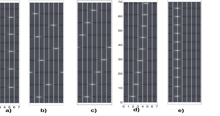
Figure 5: Density plot of $|u_{n}(t)|$ with a small loss/gain. Initial condition $u_{n}(0)=a(1+\epsilon(c_{+}e^{ikn}+c_{-}e^{-ikn}))$, where $N=7$, $a=1.1$, $\epsilon=10^{-4}$, $c_{+}=0.53-i0.86$ and $c_{-}=-0.26+i0.22$ (as in Fig 1). The integration is performed using the 6th order Runge-Kutta [57]. a) $\nu=-10^{-6}$; the system enters immediately the attractor of the loss dynamics characterized by $\Delta x=N/2$.b) $\nu=-10^{-8}$; the system enters the loss attractor after a transient of few appearences. c) $\nu=0$; pure AL dynamics. d) $\nu=10^{-8}$; the system enters the attractor of the gain dynamics, characterized by $\Delta x=0$, after a transient of few appearences. e) $\nu=10^{-6}$; the system enters immediately the attractor of the gain dynamics.

To have an idea on how good this analytic theory is in describing the FPUT recurrence of AWs in the presence of loss or gain, in the following table we compare the numerical output of the experiment described in Figure 5 b) (${\epsilon}=10^{-4},\nu=-10^{-8}$) with the above theoretical predictions:
 

	Numeric	Theor
($\Delta X_{1}$, $\Delta T_{1}$)	(2.010914,  8.671074 )	(2.010913,  8.671072)
($\Delta X_{2}$, $\Delta T_{2}$)	(2.6311495, 8.529947 )	(2.6311491, 8.529944)
($\Delta X_{3}$, $\Delta T_{3}$)	(2.9190295, 8.380007)	(2.9190291, 8.380003)
($\Delta X_{4}$, $\Delta T_{4}$)	(3.0716356, 8.256583 )	(3.0716351, 8.256578)
($\Delta X_{5}$, $\Delta T_{5}$)	(3.1626266, 8.15582 )	(3.1626261, 8.15681)

The whorst difference between numerics and the theory is in the $5^{th}$ decimal digit, while the expected error is $O({\epsilon})=O(10^{-4})$. Therefore this perturbation theory does even better than expected from theoretical arguments.

From (91) it follows that

$$(E^{+}(\lambda_{1})-E^{-}(\lambda_{1}))_{n}^{2}\to\nu\frac{8|a|^{2}\lambda_{1}^{2}\cos^{2}\phi\cos\frac{\kappa_{1}}{2}}{N(1+|a|^{2})}\sum\limits_{j=1}^{n}I(\phi,x^{(j)})$$ (102)

as $n$ increases. Therefore the gap, whose initial inclination is arbitrary, tends to become horizontal in $\nu>0$ (gain), and vertical if $\nu<0$ (loss) (see Figure 6).

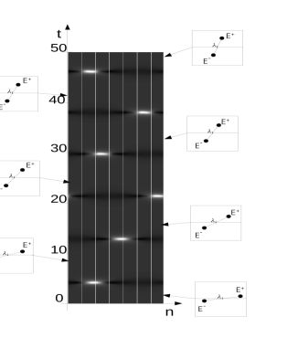
Figure 6: Density plot of $|u_{n}(t)|$ and the (discrete) evolution of the gap $E^{+}-E^{-}$, due to the AW appearence, in the case of a small loss. The numerical experiment is the same as in Figure 5 b).

3.2 Hamiltonian perturbation

In many physical contexts, a quintic term is introduced in NLS type models to describe higher order Hamiltonian effects. The matrix perturbation of the Lax pair is chosen as follows:

$$F[u_{n}]=-i\gamma\begin{pmatrix}0&u_{n}\\ \overline{u_{n}}&0\end{pmatrix}|u_{n}|^{4},\ \ |\gamma|\ll 1,$$ (103)

and the variation of $\mbox{tr}\tilde{T}$ after the $j^{th}$ appearance of the AW is described by the analytic formula

$$\begin{split}&\Delta_{j}\left(\frac{Tr(T)}{\sqrt{\det T}}\right)=-i\gamma\left(\frac{2N|a|^{6}\cos\phi_{1}\sin^{2}\phi_{1}\cos\frac{k_{1}}{2}}{1+|a|^{2}}\right)\tilde{I}(\phi_{1},x^{(j)}),\end{split}$$ (104)

$$\begin{split}&\tilde{I}(\phi_{1},x^{(j)})=\int_{-\infty}^{\infty}\sum_{n=1}^{N}\frac{{\mathcal{N}}(n,t;x^{(j)})}{{\mathcal{D}}(n,t;x^{(j)})}dt,\end{split}$$ (105)

where

$$\begin{split}&{\mathcal{N}}(n,t;x^{(j)})=\bigg{|}\cos\left(\frac{\kappa_{1}}{2}\right)\cosh(\sigma_{1}(t)+2i\phi_{1})+\sin\phi_{1}\cos\left(k_{1}(n-x^{(j)})\right)\bigg{|}^{4}\times\\ &\times\bigg{\{}\sin(k_{1}(n-x^{(j)}))\left[2\cos\frac{k_{1}}{2}\sin^{2}\phi_{1}-\cos\frac{k_{1}}{2}\cosh(\sigma_{1}t)^{2}-\sin\phi_{1}\cos(k_{1}(n-x^{(j)}))\cosh(\sigma_{1}t\right]+\\ &+i\sinh(\sigma_{1}t)\left[\cos\frac{k_{1}}{2}\cos(k_{1}(n-x^{(j)}))\cosh(\sigma_{1}t-\sin\phi_{1}\bigg{(}\cos k_{1}+\sin^{2}(k_{1}(n-x^{(j)}))\bigg{)}\right]\bigg{\}},\end{split}$$ (106)

and

$$\begin{split}&{\mathcal{D}}(n,t;x^{(j)})=\left[\cos\frac{k_{1}}{2}\cosh(\sigma_{1}t)-\cos\left(k_{1}\left(n-x^{(j)}\right)\right)\sin\phi_{1}\right]^{5}\times\\ &\times\left[\cos\frac{k_{1}}{2}\cosh(\sigma_{1}t)-\cos\left(k_{1}\left(n-x^{(j)}+1\right)\right)\sin\phi_{1}\right]\left[\cos\frac{k_{1}}{2}\cosh(\sigma_{1}t)-\cos\left(k_{1}\left(n-x^{(j)}-1\right)\right)\sin\phi_{1}\right].\end{split}$$ (107)

Proceeding as in the previous section, one obtains the same main result as before, but now

$$Q_{n}=\alpha_{1}\beta_{1}-i\frac{\gamma}{{\epsilon}^{2}}\frac{8a^{4}\cos^{3}(\phi)\sin^{2}(\phi)\cos\frac{\kappa_{1}}{2}}{N}\sum_{j=1}^{n}\tilde{I}(\phi_{1},x^{(j)}),\ \ n\geq 0.$$ (108)

As in the loss/gain case, the $x$-shifts $\Delta_{n}x$ and the recurrence times $\Delta_{n}t$ after the $n^{th}$ appearance depend, through $Q_{n}$ in (108), on the positions $x^{(j)},~{}j=1,\dots,n$ of the first $n$ AW appearances. But now this contributions are purely imaginary and their imaginary parts can be either positive or negative. Therefore one cannot have, in general, asymptotic attractors. On the other hand, if $\gamma~{}{\epsilon}^{-2}=O(1)$ as in Figure 7, then these purely imaginary terms prevail over the term $|\alpha_{1}\beta_{1}|=O(1)$ in (108), due to the quintic perturbation. Therefore, at each appearance

$$\Delta_{j}x\sim\pm\frac{N}{4}$$ (109)

(see Figure 7).

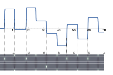
Figure 7: Dynamics of the imaginary part of trace $\Im\left(\frac{Tr(T)}{\sqrt{\det T}}\right)$, in the presence of the hamiltonian perturbation $\gamma=10^{-8}$. The variations correspond to the AW appearances. The initial condition is the same as before: $u_{n}(0)=a(1+\epsilon(c_{+}e^{ik_{1}n}+c_{-}e^{-ik_{1}n}))$, with $a=1.1$, $\epsilon=10^{-4}$, $k_{1}=\frac{2\pi}{N}$, $N=7$, $c_{+}=0.53-i*0.86$ and $c_{-}=-0.26+i*0.22$.

4 Appendix

To evaluate explicitly the right hand side of (80), the simplest way is to make use of the Darboux transformations (DTs) of the AL equations (see [18]), concentrating on the $AL_{+}$ equation.
 
Proposition [18]. Let $\left(u_{n}^{[0]},{\underline{\psi}}_{n}^{[0]}(\lambda)\right)$ be a solution of the Lax pair (4) for $\eta=1$, then $\left(u_{n}^{[1]},{\underline{\psi}}_{n}^{[1]}(\lambda)\right)$ is also a solution of (4), where

$$\begin{array}[]{l}{\underline{\psi}}_{n}^{[1]}(\lambda)=D_{n}(\lambda){\underline{\psi}}_{n}^{[0]}(\lambda),\ \ \ u_{n}^{[1]}=a_{n+1}u_{n}^{[0]}+b_{n+1},\end{array}$$ (110)

$$\begin{array}[]{l}D_{n}(\lambda)=\frac{1}{\lambda_{1}|q_{2}|^{2}+\frac{|q_{1}|^{2}}{\lambda_{1}}}\times\\ \times\begin{pmatrix}\left(\frac{\lambda}{\lambda_{1}}-\frac{\lambda_{1}}{\lambda}\right)|{q_{1}}_{n}|^{2}+\left(\lambda\lambda_{1}-\frac{1}{\lambda\lambda_{1}}\right)|{q_{2}}_{n}|^{2}&-{q_{1}}_{n}{\overline{q}_{2}}_{n}\left(\lambda_{1}^{2}-\frac{1}{\lambda_{1}^{2}}\right)\\ {q_{2}}_{n}{\overline{q}_{1}}_{n}\left(\lambda_{1}^{2}-\frac{1}{\lambda_{1}^{2}}\right)&-\left(\lambda\lambda_{1}-\frac{1}{\lambda\lambda_{1}}\right)|{q_{1}}_{n}|^{2}-\left(\frac{\lambda}{\lambda_{1}}-\frac{\lambda_{1}}{\lambda}\right)|{q_{2}}_{n}|^{2}\end{pmatrix},\end{array}$$ (111)

$$\begin{array}[]{l}a_{n}=\frac{\lambda_{1}|{q_{1}}_{n}|^{2}+|{q_{1}}_{n}|^{2}\lambda_{1}}{\lambda_{1}|{q_{2}}_{n}|^{2}-{q_{1}}_{n}|^{2}/\lambda_{1}},\ \ b_{n}=\frac{\lambda_{1}^{2}-1/\lambda_{1}^{2}}{\lambda_{1}|{q_{2}}_{n}|^{2}-|{q_{1}}_{n}|^{2}/\lambda_{1}},\end{array}$$ (112)

and ${\vec{q}}_{n}=({q_{1}}_{n},{q_{2}}_{n})^{T}$ is a linear combination of two independent solutions of (4) for $u_{n}=u_{n}^{[0]}$, evaluated at $\lambda=\lambda_{1}$, where $\lambda_{1}$ is a real parameter in the interval $(1,\lambda_{0})$ (an unstable double point) (see Figure 2).

Now we specialize this construction choosing $u^{[0]}_{n}(t)=a\,e^{2i\eta|a|^{2}t}$ (the background solution); then a matrix fundamental solution of the Lax pair (4) reads

$$\begin{array}[]{l}{\Psi}^{[0]}_{n}=\left(1+\eta\,|a|^{2}\right)^{\frac{n}{2}}e^{i\left(|a|^{2}t+\frac{\arg a}{2}\right)\sigma_{3}}\begin{pmatrix}e^{i\frac{\eta}{2}(kn-\phi)-\frac{\sigma t}{2}}&&-e^{-i\frac{\eta}{2}(kn-\phi)+\frac{\sigma t}{2}}\\ \frac{i}{\sqrt{\eta}}e^{i\frac{\eta}{2}(kn+\phi)-\frac{\sigma t}{2}}&&\frac{i}{\sqrt{\eta}}e^{-i\frac{\eta}{2}(kn+\phi)+\frac{\sigma t}{2}}\end{pmatrix}e^{i\nu\,t},\end{array}$$ (113)

where $\kappa=2\mu=\frac{2\pi}{N}$, and a linear combination of its columns leads to

$$\begin{array}[]{l}{q_{1}}_{n}=2\cos\left(\frac{\kappa(n-x_{1})+i\eta\sigma(t-t_{1})-\phi}{2}\right)e^{i\eta|a|^{2}t+i\frac{\arg a}{2}+i\nu t},\\ {q_{2}}_{n}=-2\sqrt{\eta}\sin\left(\frac{\kappa(n-x_{1})+i\eta\sigma(t-t_{1})+\phi}{2}\right)e^{-i\eta|a|^{2}t-i\frac{\arg a}{2}+i\nu t},\end{array}$$ (114)

where $x_{1},t_{1}$ are arbitrary real parameters.

Therefore (110) leads to the AW solution (11):

$$u^{[1]}_{n}(t)=-a\;e^{2i\eta|a|^{2}t}\left[\frac{\cosh(\sigma(t-T)+2i\eta\phi)+\frac{\sin\phi}{\cos\left(\frac{\kappa}{2}\right)}\cos\left(\kappa(n-X)\right)}{\cosh(\sigma(t-T))-\frac{\sin\phi}{\cos\left(\frac{\kappa}{2}\right)}\cos\left(\kappa(n-X)\right)}\right],$$ (115)

where $X=x_{1}-\frac{\eta}{2}-\frac{\pi}{2\kappa}$ and $T=t_{1}$. Correspondingly, the Darboux (dressing) matrix reads:

$$\begin{array}[]{l}D_{n}(\lambda)=\frac{1}{\lambda_{1}|q_{2}|^{2}+\frac{|q_{1}|^{2}}{\lambda_{1}}}\times\\ \times\begin{pmatrix}\left(\frac{\lambda}{\lambda_{1}}-\frac{\lambda_{1}}{\lambda}\right)|q_{1}|^{2}+\left(\lambda\lambda_{1}-\frac{1}{\lambda\lambda_{1}}\right)|q_{2}|^{2}&-q_{1}\overline{q}_{2}\left(\lambda_{1}^{2}-\frac{1}{\lambda_{1}^{2}}\right)\\ q_{2}\overline{q}_{1}\left(\lambda_{1}^{2}-\frac{1}{\lambda_{1}^{2}}\right)&-\left(\lambda\lambda_{1}-\frac{1}{\lambda\lambda_{1}}\right)|q_{1}|^{2}-\left(\frac{\lambda}{\lambda_{1}}-\frac{\lambda_{1}}{\lambda}\right)|q_{2}|^{2}\end{pmatrix}.\end{array}$$ (116)

To calculate the remaining ingredients appearing in the basic formula (80), we observe that

$$\begin{array}[]{l}T^{[1]}(n+N,n;\lambda_{1})=\Psi_{n+N}(\lambda_{1})\Psi^{-1}_{n+N}(\lambda_{1})=\displaystyle\lim_{\lambda\rightarrow\lambda_{1}}{D_{n+N}(\lambda)\,\Psi^{[0]}_{n+N}(\lambda_{1})\left(\Psi_{n}^{[0]}(\lambda_{1})\right)^{-1}D_{n}^{-1}(\lambda)}\\ =\displaystyle\lim_{\lambda\rightarrow\lambda_{1}}{D_{n+N}(\lambda)\,T^{[0]}(n+N,n,\lambda)D_{n}^{-1}(\lambda)}=\\ =\displaystyle\lim_{\lambda\rightarrow\lambda_{1}}\Big{[}\big{(}D_{n+N}(\lambda_{1})+(\lambda-\lambda_{1})\partial_{\lambda}D_{n+N}(\lambda)\big{|}_{\lambda_{1}}\big{)}\times\\ \times\big{(}T^{[0]}(n+N,n,\lambda_{1})+(\lambda-\lambda_{1})\partial_{\lambda}T^{[0]}(n+N,n,\lambda)\big{|}_{\lambda_{1}}\big{)}D_{n}^{-1}(\lambda)\Big{]}.\end{array}$$ (117)

Therefore we need to evaluate the following quantities associated with the Darboux matrix (116):

$$D_{n}(\lambda_{1})=\frac{\left(\lambda_{1}^{2}-\frac{1}{\lambda_{1}^{2}}\right)}{\lambda_{1}|{q_{2}}_{n}|^{2}+\frac{|{q_{1}}_{n}|^{2}}{\lambda_{1}}}\begin{pmatrix}\overline{{q_{2}}_{n}}\\ \overline{{q_{1}}_{n}}\end{pmatrix}({q_{2}}_{n},-{q_{1}}_{n}),$$ (118)

$$\partial_{\lambda}D_{n}(\lambda)\bigg{|}_{\lambda=\lambda_{1}}=\frac{\mbox{diag}\left(2|{q_{1}}_{n}|^{2}+|{q_{2}}_{n}|^{2}\left(\lambda_{1}^{2}+\frac{1}{\lambda_{1}^{2}}\right),-2|{q_{2}}_{n}|^{2}-|{q_{1}}_{n}|^{2}\left(\lambda_{1}^{2}+\frac{1}{\lambda_{1}^{2}}\right)\right)}{\lambda_{1}\left(\lambda_{1}|{q_{2}}_{n}|^{2}+\frac{|{q_{1}}_{n}|^{2}}{\lambda_{1}}\right)},$$ (119)

$$\begin{array}[]{l}D_{n}^{-1}(\lambda\sim\lambda_{1})=\frac{\tilde{D}}{\lambda-\lambda_{1}}+O(1),\ \ \tilde{D}:=\frac{\lambda_{1}}{2\left(\frac{|{q_{2}}_{n}|^{2}}{\lambda_{1}}+\lambda_{1}|{q_{1}}_{n}|^{2}\right)}\begin{pmatrix}{q_{1}}_{n}\\ {q_{2}}_{n}\end{pmatrix}(\overline{{q_{1}}_{n}},-\overline{{q_{2}}_{n}}),\end{array}$$ (120)

and those associated with the transition matrix of the background solution:

$$\begin{array}[]{l}T^{[0]}(n,m,\lambda,t)=\Psi^{[0]}_{n}(\lambda,t)\left(\Psi^{[0]}_{m}(\lambda,t)\right)^{-1}\\ =\left(1+\eta\,a^{2}\right)^{\frac{n-m}{2}}\begin{pmatrix}\cos(\mu(n-m))+i\sin(\mu(n-m))\frac{g_{-}+g_{+}}{g_{-}-g_{+}}&&-2i\frac{\sin(\mu(n-m))}{g_{-}-g_{+}}e^{2i|a|^{2}t+i\arg a}\\[8.53581pt] 2i\eta\frac{\sin(\mu(n-m))}{g_{-}-g_{+}}e^{-2i|a|^{2}t-i\arg a}&&\cos(\mu(n-m))-i\sin(\mu(n-m))\frac{g_{-}+g_{+}}{g_{-}-g_{+}}\end{pmatrix}\;,\end{array}$$ (121)

$$\begin{array}[]{l}\partial_{\lambda}T^{[0]}(n,m;t)=\bigg{[}\frac{(n-m)\sin\phi}{\lambda\cos\phi}\begin{pmatrix}\sin(\mu(n-m))-\cos(\mu(n-m))\frac{\sin\phi}{\cos\phi}&-\frac{\cos(\mu(n-m))}{\cos\phi}e^{2i|a|^{2}t}\\[8.53581pt] \frac{\cos(\mu(n-m))}{\cos\phi}e^{-2i|a|^{2}t}&\sin(\mu(n-m))+\cos(\mu(n-m))\frac{\sin\phi}{\cos\phi}\end{pmatrix}+\\[8.53581pt] +\frac{\sin(\mu(n-m))\cos\left(\frac{k}{2}\right)}{\lambda\sin\left(\frac{k}{2}\right)\cos^{2}\phi}\begin{pmatrix}1&-\sin\phi\;e^{2i|a|^{2}t}+\\[8.53581pt] \sin\phi\;e^{-2i|a|^{2}t}&-1\end{pmatrix}\bigg{]}\left(1+\eta\,a^{2}\right)^{\frac{n-m}{2}}\;.\end{array}$$ (122)

At last, substituting these formulas in (117), we obtain $T^{[1]}(n+N,n;\lambda_{1})$ as in (81). Acknowledgments
This research was supported by the Research Project of National Interest (PRIN) No. 2020X4T57A. It was also done within the activities of the INDAM-GNFM.

References

- [1] M. J. Ablowitz and J. F. Ladik, “Nonlinear differential-difference equations”, Jour. Math. Phys., 16 (1975), pp. 598-603.
- [2] M. J. Ablowitz and J. F. Ladik, “Nonlinear differential-difference equations and Fourier Analysis”, Jour. Math. Phys., 17 (1976), pp. 1011-1018.
- [3] M.J. Ablowitz, Z.H. Musslimani, “Integrable nonlocal nonlinear Schrödinger equation”, Phys. Rev. Lett., 110:6 (2013), 064105; doi:10.1103/PhysRevLett.110.064105.
- [4] Ablowitz, M., Prinari, B., and Trubatch, A. (2003). Discrete and Continuous Nonlinear Schrödinger Systems (London Mathematical Society Lecture Note Series). Cambridge: Cambridge University Press. doi:10.1017/CBO9780511546709.
- [5] N. Akhmediev and A. Ankiewicz, “Modulation instability, Fermi-Pasta-Ulam recurrence, rogue waves, nonlinear phase shift, and exact solutions of the Ablowitz-Ladik equation”, Phys. Rev. E 83, 046603 (2011).
- [6] N.N. Akhmediev, V.M. Eleonskii, and N.E. Kulagin, “Generation of periodic trains of picosecond pulses in an optical fiber: exact solutions”, Sov. Phys. JETP, 62:5 (1985), 894–899.
- [7] T.B. Benjamin, J.E. Feir, “The disintegration of wave trains on deep water. Part I. Theory”, Journal of Fluid Mechanics, 27:3 (1967) 417–430; doi:10.1017/S002211206700045X.
- [8] V. I. Bespalov, V. I. Talanov, “Filamentary structure of light beams in nonlinear liquids”, JETP Letters, 3:12 (1966), 307-310.
- [9] F. Coppini, P. G. Grinevich and P. M. Santini: “The effect of a small loss or gain in the periodic NLS anomalous wave dynamics. I”, Phys. Rev. E 101, 032204 (2020). DOI: 10.1103/PhysRevE.101.032204.
- [10] F. Coppini and P. M. Santini: The Fermi-Pasta-Ulam-Tsingou recurrence of periodic anomalous waves in the complex Ginzburg-Landau and in the Lugiato-Lefever equations, Phys. Rev. E 102, 062207 (2020). DOI: 10.1103/PhysRevE.102.062207
- [11] Coppini F., Grinevich P.G., Santini P.M. (2022) Periodic Rogue Waves and Perturbation Theory. In: Meyers R.A. (eds) Encyclopedia of Complexity and Systems Science. Springer, Berlin, Heidelberg. https://doi.org/10.1007/978-3-642-27737-5762-1
- [12] F. Coppini and P. M. Santini: Modulation instability, periodic anomalous wave recurrence, and blow up in the Ablowitz - Ladik lattices, ArXiv:2305.04857.
- [13] F. Coppini and P. M. Santini: The Massive Thirring Model: exact solutions and Fermi-Pasta-Ulam-Tsingou recurrence of anomalous waves. Preprint 2021 (in preparation).
- [14] A. Doliwa and P. M. Santini: Integrable dynamics of a discrete curve and the Ablowitz-Ladik hierarchy; J. Math. Phys. 36 (1995), 1259-1273 .
- [15] B.A. Dubrovin, “Inverse problem for periodic finite-zoned potentials in the theory of scattering”, Funct. Anal. Appl., 9:1 (1975), 61–62; doi:10.1007/BF01078183.
- [16] K.B. Dysthe, K. Trulsen, “Note on Breather Type Solutions of the NLS as Models for Freak-Waves”, Physica Scripta, T82, (1999) 48–52; doi:10.1238/Physica.Topical.082a00048.
- [17] G. Gallavotti (Ed.), “The Fermi-Pasta-Ulam Problem: A Status Report”, Lecture Notes in Physics, Vol. 728, Springer, Berlin Heidelberg, 2008; doi:10.1007/978-3-540-72995-2.
- [18] Xianguo Geng, Darboux Transformation of The Discrete Ablowitz–Ladik Eigenvalue Problem, Acta Mathematica Scientia, 9 (1989), 1, 21-26. doi:10.1016/S0252-9602(18)30326-6.
- [19] P.G. Grinevich, P.M. Santini, “The finite gap method and the analytic description of the exact rogue wave recurrence in the periodic NLS Cauchy problem. 1”, Nonlinearity, 31:11 (2018), 5258–5308; doi:10.1088/1361-6544/aaddcf.
- [20] P.G. Grinevich, P.M. Santini: “The finite-gap method and the periodic NLS Cauchy problem of anomalous waves for a finite number of unstable modes”, Russian Math. Surveys 74:2 211-263 (2019). DOI: https://doi.org/10.1070/RM9863.
- [21] P.G. Grinevich, P.M. Santini, “The exact rogue wave recurrence in the NLS periodic setting via matched asymptotic expansions, for 1 and 2 unstable modes”, Physics Letters A, 382:14 (2018), 973–979; doi:10.1016/j.physleta.2018.02.014.
- [22] P.G. Grinevich, P.M. Santini: P. G. Grinevich and P. M. Santini, Numerical Instability of the Akhmediev Breather and a Finite-Gap Model of It, In: V. Buchstaber, S. Konstantinou-Rizos, A. Mikhailov (eds), Recent Developments in Integrable Systems and Related Topics of Mathematical Physics. MP 2016. Springer Proceedings in Mathematics and Statistics, vol 273. Springer, Cham (Springer, Cham, 2018).
- [23] P.G. Grinevich, P.M. Santini: The linear and nonlinear instability of the Akhmediev breather, Nonlinearity 34 (2021) 8331-8358. doi.org/10.1088/1361-6544/ac3143.
- [24] P.G. Grinevich, P.M. Santini: “Phase resonances of the NLS rogue wave recurrence in the quasi-symmetric case”, Theoretical and Mathematical Physics, 196:3 (2018), 1294–1306; doi:10.1134/S0040577918090040.
- [25] K.L. Henderson, D.H. Peregrine, J.W. Dold, “Unsteady water wave modulations: fully nonlinear solutions and comparison with the nonlinear Schrödinger equtation”, Wave Motion, 29:4 (1999), 341–361; doi:10.1016/S0165-2125(98)00045-6.
- [26] C. Kharif, E. Pelinovsky, “Physical mechanisms of the rogue wave phenomenon”, Eur. J. Mech. B/ Fluids J. Mech., 22:6 (2004), 603–634; doi:10.1016/j.euromechflu.2003.09.002.
- [27] C. Kharif, E. Pelinovsky, “Focusing of nonlinear wave groups in deep water” JETP Lett., 73 (2011), 170–175.
- [28] O. Kimmoun, H.C. Hsu, H. Branger, M.S. Li, Y.Y. Chen, C. Kharif, M. Onorato, E.J.R. Kelleher, B. Kibler, N. Akhmediev, A. Chabchoub, “Modulation Instability and Phase-Shifted Fermi-Pasta-Ulam Recurrence”, Scientific Reports, 6, Article number: 28516 (2016), doi:10.1038/srep28516.
- [29] I.M. Krichever, “Methods of algebraic Geometry in the theory on nonlinear equations”, Russian Math. Surv., 32 (1977), 185–213; doi:10.1070/RM1977v032n06ABEH003862.
- [30] I.M. Krichever, “The periodic non-Abelian Toda chain and its two-dimensional generalization”; Appendix of [15].
- [31] E. A. Kuznetsov, “Solitons in a parametrically unstable plasma”, Sov. Phys. Dokl., 22 (1977), 507–508.
- [32] E. Infeld, Quantitive theory of the Fermi-Pasta-Ulam recurrence in the Nonlinear Schrödinger Equation. Phys. Rev. Lett. 47(10):717-718, 1981.
- [33] Y. Ishimori, “An integrable classical spin chain”, J. Phys. Soc. Japan 51 (1982), 3417–3418.
- [34] A. R. Its, A. G. Izergin, V. E. Korepin, and N. A. Slavnov, Temperature correlations of quantum spins, Phys. Rev. Letters, 70:11 (1991) 1704 - 1706.
- [35] A.R. Its, V.P. Kotljarov, “Explicit formulas for solutions of a nonlinear Schrödinger equation”, Dokl. Akad. Nauk Ukrain. SSR Ser. A, 1051, 965–968 (1976).
- [36] A.R. Its, V.B. Matveev, “Hill’s operator with finitely many gaps”, Funct. Anal. Appl., 9:1 (1975), 65–66; doi:10.1007/BF01078185.
- [37] A.R. Its, A.V. Rybin, M.A. Sall, “Exact integration of nonlinear Schrödinger equation”, Theor. Math. Phys., 74 (1988), 20–32; doi:10.1007/BF01018207.
- [38] P.D. Lax, “Periodic solutions of the KdV equation”, Lectures in Appl. Math., 15 (1974), 85–96.
- [39] E. Lieb, T. Schultz, and D. Mattis, “Two soluble models of an antiferromagnetic chain”, Ann. Phys. (N.Y.) 16,3, 407–446 (1961).
- [40] L. A. Lugiato and R. Lefevre, “Spatial Dissipative Structures in Passive Optical Systems”, Phys. Rev. Letters 85 (1987), pp. 2209–2211.
- [41] Y. C. Ma, “The perturbed plane wave solutions of the cubic Schrödinger equation”, Stud. Appl. Math., 60:1 (1979), 43–58;
- [42] P. Marquié, J. M. Bilbault, M. Remoissenet, “Observation of nonlinear localized modes in an electrical lattice”. Physical Review E, 51:6 (1995), 6127–6133; doi:10.1103/physreve.51.6127.
- [43] H.P. McKean, P. Van Moerbeke, “The spectrum of Hill’s equation”, Invent. Math., 30:3 (1975), 217–274; doi:10.1007/BF01425567.
- [44] A. V. Mikhailov, “Integrability of the two-dimensional Thirring model”, JETP Lett. (USSR) (Engl. Transl.) 23:6 (1976).
- [45] P. D. Miller, N. M. Ercolani, I. M. Krichever and C. D. Levermore, “Finite genus solutions to the Ablowitz–Ladik equations”, Communications on Pure and Applied Mathematics , 48 (1995) 1369-1440.
- [46] A. Mussot, C. Naveau, M. Conforti, A. Kudlinski, P. Szriftgiser, F. Copie, S. Trillo, “Fibre multiwave-mixing combs reveal the broken symmetry of Fermi-Pasta-Ulam recurrence”, Nature Photonics, 12:5 (2018), 303–308; doi:10.1038/s41566-018-0136-1.
- [47] K. Narita, “Soliton Solutions for Discrete Hirota Equation. II”, J. Phys. Soc. Jpn., 60:5 (1991), 1497–1500; doi:10.1143/JPSJ.60.1497.
- [48] A. C. Newell and J. A. Whitehead, “Review of the Finite Bandwidth Concept”, Proc. I.U.T.A.M. Symposium on Instability of Continuous Systems, Springer-Verlag, Berlin, 1969, pp. 284-289; doi:10.1007/978-3-642-65073-4_39.
- [49] S.P. Novikov, “The periodic problem for the Korteweg-de Vries equation”, Funct. Anal. Appl., 8:3 (1974), 236–246; doi:10.1007/BF01075697.
- [50] M. Onorato, S. Residori, U. Bortolozzo, A. Montina, F.T. Arecchi, “Rogue waves and their generating mechanisms in different physical contexts”, Physics Reports, 528:2 (2013) 47–89; doi:10.1016/j.physrep.2013.03.001.
- [51] A. Osborne, M. Onorato, M. Serio, “The nonlinear dynamics of rogue waves and holes in deep-water gravity wave trains”, Phys. Lett. A, 275(5-6) (2000), 386–393; doi:10.1016/S0375-9601(00)00575-2.
- [52] Y. Ohta and J. Yang, “General rogue waves in the focusing and defocusing Ablowitz-Ladik equations”, J. Phys. A: Math. Theor. 47 (2014) 255201 (23pp).
- [53] D.H. Peregrine, “Water waves, nonlinear Schrödinger equations and their solutions”, J. Austral. Math. Soc. Ser. B, 25 (1983), 16–43; doi:10.1017/S0334270000003891
- [54] D. Pierangeli, M. Flammini, L. Zhang, G. Marcucci, A.J. Agranat, P.G. Grinevich, P.M. Santini, C. Conti, E. DelRe, “Observation of exact Fermi-Pasta-Ulam-Tsingou recurrence and its exact dynamics”, Phys. Rev. X, 8:4, p. 041017 (9 pages); doi:10.1103/PhysRevX.8.041017.
- [55] B. Prinari, “Discrete solitons of the focusing Ablowitz-Ladik equation with nonzero boundary conditions via inverse scattering”. Journal of Mathematical Physics, 57(8), 083510 (2016). doi:10.1063/1.4961160
- [56] P.M. Santini, “The periodic Cauchy problem for PT-symmetric NLS, I: the first appearance of rogue waves, regular behavior or blow up at finite times”, J. Phys. A: Math. Theor., 51:49 (2018), 495207 (21pp); doi:10.1088/1751-8121/aaea05.
- [57] D. Sarafyan, ”Improved sixth-order Runge-Kutta formulas and approximate continuous solution of ordinary differential equations”, Journal of Mathematical Analysis and Applications, 40 (1972) 436-445. doi:10.1016/0022-247X(72)90062-5.
- [58] D.R. Solli, C. Ropers, P. Koonath and B. Jalali, “Optical rogue waves”, Nature, 450 (2007), 1054–1057; doi:10.1038/nature06402.
- [59] J.M. Soto-Crespo, N. Devine, and N. Akhmediev, Adiabatic transformation of continuous waves into trains of pulses, Phys. Rev. A 96, 023825 (2017).
- [60] G. Stokes, “On the Theory of Oscillatory Waves”, Transactions of the Cambridge Philosophical Society VIII (1847) 197–229, and Supplement 314–326.
- [61] S. Takeno and K. Hori, “A propagating self-localized mode in a one-dimensional lattice with quartic anharmonicity”, J. Phys. Soc. Japan, 59 (1990), 3037–3040 .
- [62] W. E. Thirring, “A soluble relativistic field theory”. Annals of Physics, 3 (1958) 91–112. doi:10.1016/0003-4916(58)90015-0
- [63] S. Trillo and S. Wabnitz, Dynamics of the nonlinear modulational instability in optical fibers, Optics Letters, 16 (13): 986-988, 1991.
- [64] G. Van Simaeys, P. Emplit, M. Haelterman, “Experimental Demonstration of the Fermi-Pasta-Ulam Recurrence in a Modulationally Unstable Optical Wave”, Phys. Rev. Lett., 87:3 (2001), 033902; doi:10.1103/PhysRevLett.87.033902.
- [65] H.C. Yuen, W.E. Ferguson, “Relationship between Benjamin-Feir instability and recurrence in the nonlinear Schrödinger equation”, Phys. Fluids, 21:8 (1978), 1275–1278; doi:10.1063/1.862394.
- [66] H. Yuen, B. Lake, “Nonlinear dynamics of deep-water gravity waves”, Advances in Applied Mechanics, 22 (1982) 67–229; doi:10.1016/S0065-2156(08)70066-8.
- [67] A.V. Yurov, and V.A. Yurov, The Landau-Lifshitz Equation, the NLS, and the Magnetic Rogue Wave as a By-Product of Two Colliding Regular “Positons”, Symmetry, 10, 82 (2018). doi:10.3390/sym10040082.
- [68] V.E. Zakharov, “Stability of period waves of finite amplitude on surface of a deep fluid”, Journal of Applied Mechanics and Technical Physics, 9:2 (1968) 190–194.
- [69] V. Zakharov, L. Ostrovsky, Modulation instability: the beginning, Physica D: Nonlinear Phenomena, 238:5 (2009), 540–548; doi:10.1016/j.physd.2008.12.002.
- [70] V.E. Zakharov, A.B. Shabat, “Exact theory of two-dimensional self-focusing and one-dimensional self-modulation of waves in nonlinear media”, Sov. Phys. JETP, 34:1 (1972), 62–69.