Observational predictions for Thorne–Żytkow objects

Abstract

Thorne–Żytkow objects (TŻO) are potential end products of the merger of a neutron star with a non-degenerate star. In this work, we have computed the first grid of evolutionary models of TŻOs with the MESA stellar evolution code. With these models, we predict several observational properties of TŻOs, including their surface temperatures and luminosities, pulsation periods, and nucleosynthetic products. We expand the range of possible TŻO solutions to cover $3.45\lesssim\rm{\log\left(T_{eff}/K\right)}\lesssim 3.65$ and $4.85\lesssim\rm{\log\left(L/L_{\odot}\right)}\lesssim 5.5$. Due to the much higher densities our TŻOs reach compared to previous models, if TŻOs form we expect them to be stable over a larger mass range than previously predicted, without exhibiting a gap in their mass distribution. Using the GYRE stellar pulsation code we show that TŻOs should have fundamental pulsation periods of 1000–2000 days, and period ratios of $\approx$0.2–0.3. Models computed with a large 399 isotope fully-coupled nuclear network show a nucleosynthetic signal that is different to previously predicted. We propose a new nucleosynthetic signal to determine a star’s status as a TŻO: the isotopologues $\mathrm{{}^{44}Ti}\rm{O}_{2}$ and $\mathrm{{}^{44}Ti}\rm{O}$, which will have a shift in their spectral features as compared to stable titanium-containing molecules. We find that in the local Universe ($\sim$SMC metallicities and above) TŻOs show little heavy metal enrichment, potentially explaining the difficulty in finding TŻOs to-date.

1 Introduction

Thorne–Żytkow objects (TŻOs) are the hypothetical unique product of the merger of a neutron star (NS) with a non-degenerate star leading to the formation of a single object (Thorne & Zytkow, 1975, 1977). Depending on the mass of the combined star, it can be supported either via nuclear burning on/or near the surface of the NS and by accretion onto the NS (Eich et al., 1989; Biehle, 1991).

A number of potential TŻOs candidates have been suggested: U Aqr (Vanture et al., 1999), HV 2112 (Levesque et al., 2014), HV 11417 (Beasor et al., 2018), and VX Sgr (Tabernero et al., 2021), though they are not without controversy (Coe & Pightling, 1998; Vanture et al., 1999; Tout et al., 2014; Maccarone & de Mink, 2016; Tabernero et al., 2021). Objects have been also been proposed that may form a TŻO (TIC 470710327 Eisner et al. 2022), or may be the remnants of a TŻO (1E161348-5055 Liu et al. 2015). The issue with identifying a TŻO is distinguishing it from other similar stars, such as asymptotic giant branch (AGB) or super-AGB (SAGB) stars (Biehle, 1991, 1994; O’Grady et al., 2020, 2023). TŻOs are expected to appear as cool red supergiants (RSG) (Cannon et al., 1992) (hereafter C92), though many challenges remain in observing and modelling RSGs complicating their analysis (Levesque et al., 2005; Davies et al., 2018). Observations to date have relied on indirect measurements, such as their predicted unique nucleosynthetic signatures (Biehle, 1994; van Paradijs et al., 1995). Future gravitational wave observations may provide an opportunity to detect either the formation of the TŻO (Nazin & Postnov, 1995; Morán-Fraile et al., 2023), a rotating NS inside a TŻO (DeMarchi et al., 2021), or a post-TŻO black hole (BH) (Cholis et al., 2022).

TŻOs are expected to be fully convective down to a “knee” where it then transitions to a flat temperature profile until the material reaches the surface of the NS (Eich et al., 1989). At the knee, nuclear-processed material will be mixed outwards into the convective envelope, while fresh hydrogen is mixed into the region below the knee. Material may also be burnt at the base of the convective envelope. It is expected that the material is burnt via the interrupted rapid proton process (irp-process, Cannon 1993 hereafter C93), where rapid proton captures (Wallace & Woosley, 1981; van Wormer et al., 1994; Fisker et al., 2008) are interrupted when the material is mixed outwards by convection. This material then beta decays before being mixed back into the inner regions where additional proton captures can occur.

This irp-process can lead to the production of heavy elements such as Rubidium, Strontium, Yttrium, and Molybdenum (C93). It is also expected that the TŻOs will be enriched in $\mathrm{{}^{40}Ca}$ (Biehle, 1991, 1994), which in normal stars is difficult to produce and mix to the surface (Tout et al., 2014). Lithium is also expected to be produced via $\mathrm{{}^{3}He}$($\alpha,\gamma$)$\mathrm{{}^{7}Be}$($e^{-},\nu$)$\mathrm{{}^{7}Li}$ (Cameron, 1955). In non-TŻO stars the $\mathrm{{}^{7}Li}$ would be destroyed by high temperatures inside the star, but in a fully convective star the $\mathrm{{}^{7}Be}$ can be mixed outwards to cooler regions before it captures an electron (Podsiadlowski et al., 1995). However, the nucleosynthetic signal is not unique, there are also TŻO imposters: SAGB stars (Kuchner et al., 2002), or stars polluted by the winds of a SAGB star and are now an AGB themselves (Maccarone & de Mink, 2016), which may have similar nucleosynthetic signals to a TŻO.

There are a number of potential formation mechanisms of TŻOs: engulfment of the NS during a common envelope (Taam et al., 1978; Terman et al., 1995; Ablimit et al., 2022); the NS receiving a kick such that it has a direct impact with the companion (Leonard et al., 1994); or a dynamical merger either in a dense stellar cluster (Ray et al., 1987) or a triple system (Eisner et al., 2022). The formation of a TŻO is likely to produce a transient event (Hirai & Podsiadlowski, 2022). Finally, TŻOs are expected to die either when they run out of rp-seed material to burn forcing the material near the NS to heat up and enter the pair-instability region. This causes a runaway increase in the neutrino losses, causing the accretion onto the NS to no longer be Eddington limited, and the NS collapses into a BH (Podsiadlowski et al., 1995). This may possibly form a transient event (Moriya, 2018; Moriya & Blinnikov, 2021). Alternatively, they may eject their envelope via wind mass loss, leaving behind a “bare” NS (Bisnovatyi-Kogan & Lamzin, 1984).

The number of TŻOs in the Galaxy will depend on the rate of mergers, the fraction of mergers that successfully produce a TŻO, and the lifetime of the resulting TŻO. Podsiadlowski et al. (1995) estimated a birth rate of $>10^{-4}\,\rm{yr}^{-1}$ from common-envelope evolution, and $\sim 10^{-4}\,\rm{yr}^{-1}$ from NS kicks. Renzo et al. (2019) calculated the rate of collision from a NS being kicked during a SN with a companion to be $\approx 10^{-4}$ the core-collapse SN rate. While Ablimit et al. (2022) calculated formation rates of the merger of a ONeMg WD with a non-degenerate companion, where the core collapses and forms a NS, as between $\sim 10^{-5}$–$10^{-4}\,\rm{yr}^{-1}$. Population synthesis calculations have shown an expected merger rate of a NS with a giant star as high as $\approx 1$ per 100 core-collapse supernovae, depending on the assumed physics of the common envelope merger (Grichener, 2023). N-body simulations of globular clusters show dynamical mergers of a NS with main sequence star at a rate of the order 1 per $\sim 4000$ NS containing binaries (Kremer et al., 2020). The actual formation rate of TŻOs will however depend on the probability that the merger is successful and does not lead to a transient or complete disruption of the system (Schrøder et al., 2020).

The first models of TŻOs presented in Thorne & Zytkow (1975, 1977) were equilibrium models. Here the TŻO was split into three regions: an outer region which encompasses the envelope down to the knee; a middle region between the knee and the surface of the NS; and an inner region for the NS itself. These models were not evolved in time; instead, static solutions where found based on the assumed NS and envelope properties. Biehle (1991) improved on the static models by including a simplified model of rp-burning, instead of just assuming CNO burning. Finally, C92 & C93 created a set of evolutionary models where the NS was modelled by altering the EOS such that the electrons become increasingly degenerate in the vicinity of the NS. However, these models ignored wind mass loss and ignored changes in the composition.

In Section 2 we show how we build a TŻO in MESA and discuss our default model. In Section 3 we show the evolution of a grid of TŻO models. In Section 4 we make predictions for the expected pulsation signal. In Section 5 we explore the nucleosynthetic signal from TŻOs. We discuss the suitability of our model assumptions in Section 6, and show the possible final fates of TŻOs in Section 7. Finally, we discuss our results in Section 8 and conclude in Section 9.

2 Building a TŻO model

Realistic modelling of the formation of a TŻO is a complex multi-dimensional problem involving the merger of a NS with the core of another star. In this work, we ignore both the NS and the merger process. Doing so, we construct a spherically symmetric post-merger structure of the envelope of the TŻO that is then allowed to evolve. There are three phases to creating our models: 1) producing an initial seed model, 2) modifying the inner boundary of our models, and 3) adjusting the global parameters of the model to match a chosen set of starting conditions. Our inlists and models are available at https://doi.org/10.5281/zenodo.4534425. An example model is also available in MESA’s star/test_suite as of version a7c411b1.

2.1 Seed model

Using MESA r22.11.1 (Paxton et al., 2011; Paxton et al., 2013, 2015, 2018, 2019; Jermyn et al., 2023) we evolve a 20$\,\rm{M}_{\odot}$ star from the pre-main sequence until midway through the main sequence (MS). This model is used to initialise the stellar structure equations for all TŻOs, independent of their final mass and composition. The precise choice of physics does not matter here, as the formation process will wipe away any knowledge the model had of its pre-TŻO state.

2.2 Adjusting the inner boundary

With our initial stellar model, we then model the NS by adjusting the inner boundaries of the stellar model. We gradually increase the inner mass, radius, and luminosity at the inner boundary of the model using MESA’s relax_core method. This gradually changes the inner boundary while smoothly increasing the core density and core energy generation rate. By changing the inner mass boundary we do not change the total mass of the star, thus after forming a TŻO, we assume the total mass remains constant.

2.3 Starting conditions

With the base TŻO formed, we then further alter the model to match our required starting conditions. We use MESA’s relax_mass to add (remove) mass via wind accretion (loss) to alter the total mass of the TŻO. We then change the initial metal composition $\rm{Z_{init}}$, assuming a solar-scaled composition, and the initial helium fraction $\rm{Y_{init}}$with relax_composition. This allows us to build a TŻO with an arbitrary initial mass and composition, which can be used to approximate the post-merger structure for different formation scenarios.

We allow for arbitrary helium compositions, as the merger between a NS and a star may occur at any point in the star’s lifetime (ignoring selection effects in terms of which stars are likely to successfully merge and form a TŻO). If a TŻO forms from a NS kick or a dynamical merger then the age of the companion star is a free parameter, while mergers from a common envelope will likely, but not necessarily, involve the companion star having evolved beyond the MS. The mixing of the helium produced in the centre of a MS/post-MS star into the envelope will raise the helium mass fraction of the TŻO envelope compared to a canonical RSG. Mass loss from the envelope of the star during the merger will likely preferentially remove H-rich material and thus increase the average helium content of the TŻO. Thus when the star is fully mixed the average helium content over the entire star will increase. In the limit of when the entire hydrogen envelope is removed, a pure helium TŻO could be formed if it survives the merger process. However, whether a TZO may form from the merger of a NS with an evolved star or not is even more uncertain than TŻO formation with main sequence stars (Papish et al., 2015; Metzger, 2022).

At this point, we can also set other physics options, such as the choice of the nuclear network, accretion rate onto the NS, wind mass loss efficiency, or the mixing length. These are discussed further in Appendix A. Although orbital angular momentum is involved in the merger process, the amount retained post-merger is still an open question (e.g., Schneider et al., 2019). Thus, for simplicity, in this work we consider only non-rotating models.

2.4 Default TŻO model

Here we describe our default TŻO model and the choices for uncertain physical and numerical quantities we have made. The effect of varying these choices is explored further in Appendix A. We assume a default NS mass of $M_{\rm NS}=1.4\,\,\rm{M}_{\odot}$. The radius of a NS is still uncertain and depends on the chosen NS equation of state (EOS) (Steiner et al., 2010; Miller et al., 2019). A realistic assumption would be to assume $R_{\rm{NS}}=10$–$20\,\mathrm{k}\mathrm{m}$ for the radius of the NS and use that as the inner boundary of our model. However, we have found that to be numerically difficult to model. Thus we move the inner boundary out to a radius of $\approx 650\,\mathrm{k}\mathrm{m}$. This implies an average core density of $\langle\rho_{c}\rangle=10^{9.3}\,\mathrm{g}\,{\mathrm{c}\mathrm{m}}^{-3}$, instead of $\langle\rho_{c}\rangle\approx 10^{14}\,\mathrm{g}\,{\mathrm{c}\mathrm{m}}^{-3}$ for a $10\,\mathrm{k}\mathrm{m}$ NS.

To compensate for the fact that we do not fully calculate the structure of the TŻO down to the surface of the NS, we inject energy at the inner boundary of our model. This energy injection approximates the missing energy generated from accretion and nuclear burning below the knee in the “middle” region. These assumptions are tested in Section 6. We parameterise this inner energy injection based on the Eddington luminosity onto the NS as:

$$L_{\rm{knee}}=\epsilon_{L}L_{\rm Edd}$$ (1)

where the Eddington luminosity, $L_{\rm Edd}$, is:

$$L_{\rm Edd}=\frac{4\pi cGM_{\rm NS}}{\kappa_{c}}$$ (2)

with $G$ the standard gravitational constant, $M_{\rm NS}$ is the mass of the neutron star, $c$ is the speed of light, and $\kappa_{c}$ of the opacity of the material at the inner boundary of the model. $L_{\rm{knee}}$ is allowed to evolve with time as the mass of the NS and the opacity at the inner boundary of the TŻO changes. Finally, $\epsilon_{L}$ is an efficiency factor, for which by default we use $\epsilon_{L}=1.0$. We use $L_{*}$ to denote the outer surface luminosity of our models.

By parameterising the energy in this way we can control how deep below the knee we model. The point where the local luminosity $L>L_{\rm Edd}$ is the point where radiation can no longer carry the energy and the envelope becomes convective. Thus when $\epsilon_{L}=1.0$ the inner boundary of the structure we are calculating corresponds to the knee, which is also the base of the convection zone (C93). Smaller values of $\epsilon_{L}$ include more of the material below the knee in the calculation but come at a greater computational cost. By injecting energy in this way we are assuming that the material below the knee is actually able to generate that much energy. It is possible that some of our models would not be able to do this, in which case the corresponding TŻO may not form. We are also assuming that the material below the knee is not mixed into the envelope, which may change the nucleosynthetic signatures.

We assume the NS grows at a rate set by the Eddington accretion rate on the NS:

$$\dot{M}_{\rm Edd}=\epsilon_{\dot{M}}\frac{L_{\rm Edd}}{c^{2}}$$ (3)

where $\epsilon_{\dot{M}}$is a scale factor which by default we set as $\epsilon_{\dot{M}}=1.0$. This leads to typical accretion rates of $\sim 10^{-8}\,\rm{M}_{\odot}\,\rm{yr}^{-1}$ for $\epsilon_{\dot{M}}=1$.

Our default model assumes an initial metallicity of $\rm{Z_{init}}=10^{-4}$ and initial helium fraction $\rm{Y_{init}}=0.28$. Our default TŻO has an initial total mass of $\rm{M_{init}}=5\,\,\rm{M}_{\odot}$, which includes a default NS $M_{\rm NS}=1.4\,\,\rm{M}_{\odot}$, thus having an envelope mass of 3.6$\,\rm{M}_{\odot}$. After 100 years of evolution, we enable MESA’s hydrodynamic capabilities (Paxton et al., 2015). This wait is to allow the star to return to gravothermal equilibrium after the TŻO formation process. We also explore a series of model grids of TŻOs with masses between $\rm{M_{init}}=5$–20$\,\rm{M}_{\odot}$, $\rm{Z_{init}}=10^{-5}$–0.03, and $\rm{Y_{init}}=0.28$–0.65.

We conservatively stop our models once the velocity of the surface layers exceeds 10% of the escape velocity. At this stage the models undergo RSG pulsations, where there are large-amplitude surface pulsations which cause spiral patterns (Heger et al., 1997) in a Hertzsprung-Russell diagram (HRD). This can change the stellar radius by factors of $\approx 2$ over timescales of years. At this point the envelope begins expanding and contracting supersonically, and can reach $\sim 40\%$ of the escape velocity before we can longer follow the evolution. These pulsations are resolvable in models of RSGs in MESA when the timestep becomes much shorter ($\sim$days) than the pulsation timescale ($\sim$years) (Paxton et al., 2013). The timestep becomes this small due to changes in the nuclear burning (see Section 4.2). While the evolution can be continued beyond this point by suppressing the hydrodynamics either globally or only in the cool outer envelope, the results become numerically unstable. More work is needed to determine how to couple the instabilities in the nuclear burning with the pulsational instabilities in the envelope.

We evolve the majority of our models using MESA’s approx21.net nuclear network. This contains the main PP, CNO, and alpha capture reactions up to $\mathrm{{}^{56}Fe}$. This is a computational convenience. While TŻOs are expected to undergo irp-burning, most of the energy is generated via CNO burning. We also test a large 399 nuclear network for a limited set of models. This network was built by first adding all stable isotopes up to $\mathrm{Ru}$, then adding an additional neutron to the heaviest stable isotope for each element included. We then added all proton-rich isotopes with half-lives $>1$s. Finally, there was some hand tuning to make sure there were sufficient beta-decay pathways for all isotopes, as well as adding the light isotopes needed for PP, CNO, and the CNO breakout reactions. This network is available in the online Zenodo material.

We assume a mixing-length alpha parameter of $\rm{\alpha_{mlt}}=1.8$, and use MESA’s time-dependent convection (TDC) mixing treatment (Jermyn et al., 2023). TDC has been shown to improve numerical stability during dynamical phases of evolution while reducing to the standard Cox-MLT prescription (Cox & Giuli, 1968) over longer timescales (Jermyn et al., 2023). In models that have material below the base of the convection zone (when $\epsilon_{L}<1.0$), we assume that there is an additional weak mixing process occurring, with a diffusion coefficient of $10^{6}\,\rm{cm^{2}/s}$ in the material below the knee. This helps to prevent compositional gradients from building up near the surface of the NS (Piro & Bildsten, 2007; Keek et al., 2009). We do not include convective overshoot, semiconvective, or thermohaline mixing, as the star is almost fully convective.

Our EOS for the stellar component of the TŻO is a combination of freeEOS (Irwin, 2004), HELM (Timmes & Swesty, 2000), and Skye (Jermyn et al., 2021). We make no assumptions about the NS EOS, as we can not make models with $10\lesssim R_{\rm NS}/\mathrm{k}\mathrm{m}\lesssim 20$, where NS radii are expected to be. We use the wind prescription of van Loon et al. (2005), which is based on observations of cool, dusty AGB & RSG stars, with a wind scaling factor of $\eta_{\rm{\rm VL}}=1.0$. This leads to typical wind mass loss rates of $\rm{\dot{M}}\approx 10^{-5}$–$10^{-4}\,\rm{M}_{\odot}\,\rm{yr}^{-1}$.

MESA does not include any general relativistic (GR) correction factors. For this work, we add a GR correction factor to correct the continuity equation (Thorne, 1977; Ayasli & Joss, 1982). This prescription adjusts the gravitational constant, $G$, as a function of the mass coordinate inside the star. All masses in this work are baryonic. Other MESA choices are specified in Appendix C and all options can be found in the online Zenodo inlists.

Our models have on average $\approx 1700$–$2000$ mesh points and we artificially cap the maximum timestep to be $\delta t=2\times 10^{8}\,\rm{s}$ ($\approx 6$ years). While models can take longer timesteps, this comes at the cost of an increased number of timesteps that needed to be rejected and taken again with a smaller $\delta t$ as MESA could not find a valid solution that satisfies our required numerical constraints. Variations in spatial and temporal resolution of by factors of two smaller/larger lead to changes of order $\Delta\log\left(\rm{L_{*}/L_{\odot}}\right)\approx 0.01\,\rm{dex}$.

3 Structure and evolution of a TŻO

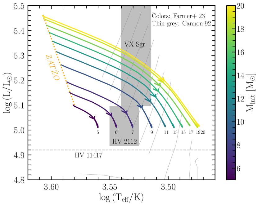
Figure 1: Hertzsprung-Russell diagram (HRD) of the TŻO as a function of their initial mass, at fixed initial composition. Models are evolved with our default assumptions and a $M_{\rm NS}=1.4\,\,\rm{M}_{\odot}$. Colours indicate the initial mass of the TŻOs. The direction of evolution is always towards decreasing luminosity. The grey boxes show the observational constraints on HV 2112 (Levesque et al., 2014) and VX Sgr (Tabernero et al., 2021). The horizontal dashed grey line shows the quoted luminosity of HV 11417 (Beasor et al., 2018), which has a variability amplitude of $\Delta m=1.86$ (Soszyński et al., 2009). The grey lines show the models of C92, where evolution is always to increasing luminosity. Arrows mark the midpoint of the TŻOs lifetime.

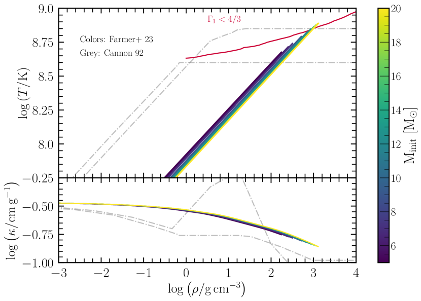
Figure 2: Top-panel: Temperature-density profiles our of our default TŻO models as a function of initial mass, at fixed initial composition. Models are evolved with our default assumptions and a $M_{\rm NS}=1.4\,\,\rm{M}_{\odot}$. Colours indicate the initial mass of the TŻOs. Dash-dotted lines show Model A and C from figures 6 and 7 of C92. Bottom-panel: The opacity as a function of the density inside the star, dash-dotted lines are from tables 1 and 2 of C92. Models shown are $\approx 40,000$ years post TŻO formation. The red line marks the edge of the pair-instability region where electron-positron production becomes significant.

Figure 1 shows the evolution of the surface temperature and luminosity of our default TŻO models. Figure 1 shows the models once they are at least 100 years old (when we turn on the hydrodynamics), where they start from a zero-age TŻO (ZATŻO) line. The endpoint of the models will be discussed further in Section 7, as shown it is when the evolution reaches 1000 years before we can no longer follow the evolution. We can see that models with higher initial masses have higher initial luminosities and temperatures compared to lower-mass models. Higher-mass models also evolve to lower final surface temperatures and live longer.

Contrary to the models of C92 our models always evolve to lower luminosities. The total luminosity of our TŻOs is a combination of the injected energy, $L_{\rm{knee}}$, and nuclear burning above the knee. The nuclear burning above the knee provides $\approx 1\%$–$10\%$ of the total luminosity, and this fraction decreases with time as the knee cools. Thus the evolution is driven by changes in $L_{\rm{knee}}$, where $L_{\rm{knee}}\propto M_{\rm NS}/\kappa_{c}$. The accretion rate on to the NS is $10^{-9}$–$10^{-8}\,\rm{M}_{\odot}\,\rm{yr}^{-1}$, which combined with a lifetime of $\approx 100,000$ years means the NS can only gain $10^{-4}$–$10^{-3}\,\,\rm{M}_{\odot}$. Thus the evolution of our TŻOs can be approximated as entirely driven by the increase in the opacity of material at the knee, which lowers $L_{\rm{knee}}$.

The opacity for the material at the knee is provided by Compton scattering (Poutanen, 2017) and thus depends on the number of free electrons per nucleon. Three factors will drive the evolution of the number of free electrons: H burning into He will decrease the number of free electrons, proton captures in rp-burning will decrease the number of nucleons, and $e^{\pm}$ production will increase the number of free electrons. If we turn off composition changes from nuclear burning (by setting dxdt_nuc_factor=0) while preserving the energy generated from nuclear burning, we find $L_{\rm{knee}}$ still decreases. However, it does this at a much faster rate than when the composition is allowed to change. Therefore, nuclear burning slows the decrease in $L_{\rm{knee}}$ but can not stop it. Thus, the changes in $L_{\rm{knee}}$ are driven by the production of $e^{\pm}$ pairs, while not entering the pair-instability region.

Our results differ from those of C92 due to differences in the chosen stopping criteria. Our models stop when supersonic pulsational instabilities form in the envelope, preventing MESA from continuing the evolution. The end condition for C92 is when the NS grows to the Oppenheimer-Volkoff (OV) (Oppenheimer & Volkoff, 1939) mass limit for the their assumed EOS, which for C92 is 2$\,\rm{M}_{\odot}$. As the NS mass increases, $L_{\rm{knee}}$ will increase, increasing the total luminosity of the star in agreement with the results of C92. However, our models stop significantly earlier than C92 such that the NS only gains $10^{-4}$–$10^{-3}\,\,\rm{M}_{\odot}$, which does not cause $L_{\rm{knee}}$ to increase by a significant amount. We note in passing that C92 states they can take single timesteps of $\approx 10^{5}$ years, which is comparable to the entire lifetime of many of our models which is between 50,000 and 200,000 years for the TŻOs shown in figure 1.

We can replicate the results of C92 by increasing the accretion rate onto the NS. If the accretion rate onto the NS is high enough that the mass of the NS can grow significantly (at least $\approx 0.1\,\,\rm{M}_{\odot}$) then $L_{\rm Edd}$ will increase in time. This causes the TŻO to become more luminous and more closely follow the tracks of C92, though still at higher surface temperatures and lower surface luminosities. This requires accretion rates of between $10^{3}$–$10^{4}\,\dot{M}_{\rm Edd}$ (See Appendix A). The remaining differences between our models can likely be attributed to changes in the microphysics (EOS, opacities, and nuclear reaction rates) and choice of metallicity.

Figure 2 shows the temperature-density profile and opacity-density profile inside our TŻOs arbitrarily at $\approx 40,0000$ years after TŻO formation. As the initial mass of the model increases the density also increases and the models reach higher temperatures at the base of the convection zone. Our models do not form a knee, due to the energy injection at the inner boundary of the models, so we are only modelling material above the knee. The dash-dotted lines show models A & C of C92. We can see that our models are significantly denser (by a factor $\approx 100$) than previously predicted, though this is still a factor $\approx 100$ less dense than a typical AGB/RSG.

None of our models ever evolve significantly into the pair-instability region (where $\Gamma_{1}<4/3$). Instead, models evolve around the edge of the pair-instability region (See Section 6). Note that the temperature and density of the knee evolves with time, but always stays outside of the pair-instability region.

The bottom panel of Figure 2 shows the opacity of our models in colour, and models A & C of C92 with grey dash-dotted lines. When $\log(\rho/\mathrm{g}\,{\mathrm{c}\mathrm{m}}^{-3})\leq 0.0$ our models have slightly higher opacities, as they are cooler for the same density. Once $\log(\rho/\mathrm{g}\,{\mathrm{c}\mathrm{m}}^{-3})>0.0$ our models have higher opacities than model A, but lower opacities than those of model C (which enters the pair-instability region and so $e^{\pm}$ production dominates the opacity).

In C93 they find a set of “high” and “low” mass solutions, which depends on how the energy is generated at the knee, and the production of $e^{\pm}$ due to models entering the pair-instability region which changes the required $L_{\rm{knee}}$ as the opacity increases (these are also the “giant” and “supergiant” models of Thorne & Zytkow 1977). C93 finds a gap where, for certain masses, models are unable to produce sufficient energy to keep the envelope convective. Our models do not exhibit this “luminosity gap” (which can be mapped into a mass gap) in the mass distribution of TŻOs. This is due to the higher density of our models, such that they do not enter the pair-instability region. Therefore our models would not be limited by the same mechanism as proposed by C93 and thus we should not expect a split into “high” and “low” mass solutions, even if we did model the knee. C92 also finds valid solutions for all masses, where C93 attributes this difference due to changes in the nuclear reaction rates used.

3.1 Composition effects

Figure 3 shows the average metal fraction of our TŻOs as a function of time since the TŻO formed. These models start at $Z=10^{-4}$ but can increase their total metal fractions by factors of 10-100 within $\approx 10,000$–100,000 years. Higher initial mass models evolve to higher total metal fractions, reaching near solar values for their total metallicity, though this is a significantly non-solar scaled composition. They also evolve faster to higher metallicities than the low-mass models and live longer. The ages shown are only lower limits on the lifetime of a TŻO (see Section 7), but likely lead to lifetimes of $\approx 10^{4}$–$10^{5}$ years.

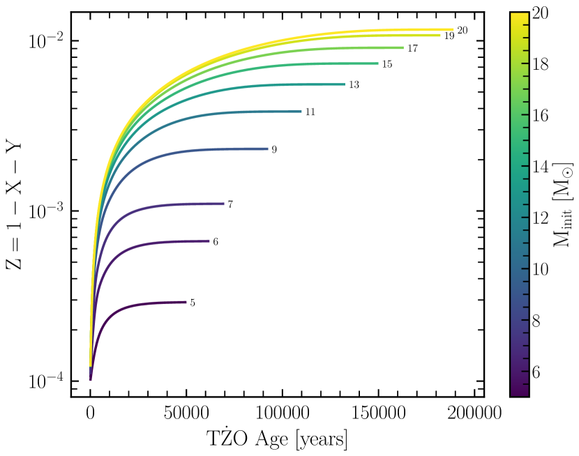
Figure 3: The evolution with time of the average metal fraction (Z) as a function of the initial mass, at fixed initial composition. Models are evolved with our default assumptions and $M_{\rm NS}=1.4\,\,\rm{M}_{\odot}$. Colours indicate the initial mass of the TŻOs. The final ages of these models are only lower limits to the lifetime of a TŻO.

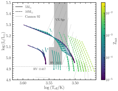
(a) Initial metallicity

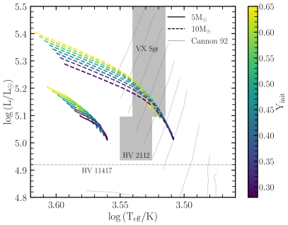
(b) Initial helium fraction

Figure 4: HRD for variations in the initial metallicity (panel a) and initial helium fraction (panel b). Solid lines denote a $5\,\,\rm{M}_{\odot}{}$ TŻO, while dashed lines denote a $10\,\,\rm{M}_{\odot}{}$ TŻO. Grey lines and grey boxes have the same meaning as in Figure 1.

Figure 4(a) shows the HRD of TŻOs with varying $\rm{Z_{init}}$ with initial masses of 5 and 10$\,\rm{M}_{\odot}$. The TŻOs can be broken into two groups of behaviour, a low initial metallicity and a high initial metallicity behaviour. The exact initial metallicity at which this behaviour changes depends on the initial mass, for the 5$\,\rm{M}_{\odot}$ models this is at $\rm{Z_{init}}\approx 3\times 10^{-4}$ while for the 10$\,\rm{M}_{\odot}$ models this occurs at $\rm{Z_{init}}\approx 10^{-3}$. This limit is approximately the final metallicity shown for each mass in Figure 3 (though the match is not exact). Effectively the low-metallicity models evolve up to the mass dependent critical $Z$, with the evolution converging to the same final surface temperature and luminosity once they reach the critical $Z$. In contrast, the models that start with metallicities above this critical limit follow their own $Z$-dependent evolutionary tracks. We can also see in Figure 4(a) that the high-metallicity models evolve along similar tracks independent of the initial mass (except for their starting luminosities). We also note that as the initial metallicity increases the 5$\,\rm{M}_{\odot}$ models are more likely to become numerically unstable.

As the metallicity increase (either due to a higher initial metallicity or due to metals produced from nuclear burning), the opacity at the knee increases (Xin et al., 2022). This decreases $L_{\rm{knee}}$ and thus decreases the temperature at the knee. This decreases the amount of heavy metal burning as the metallicity increases, though the rate of CNO burning increases as the metallicity increases due to the increased amount of CNO material. Thus the nuclear burning luminosity is greater in the high metallicity models, but the rate of production of all metals is lower. Hence at LMC and SMC metallicites TŻOs may show little metal enrichment. The high metallicity models can have lifetimes up to a factor $\approx 2$ more than shown in Figure 3.

Figure 4(b) shows variations in the initial helium fraction $\rm{Y_{init}}$, for a 5 and 10$\,\rm{M}_{\odot}$ TŻO at $\rm{Z_{init}}=10^{-4}$. As the initial helium fraction increases, the models become more luminous and have higher surface temperatures. The variation in the initial helium fraction may be expected due to variations in the evolutionary state of the companion when the TŻO merger takes place. As $\rm{Y_{init}}$ increases the final luminosity they reach increases and is at higher surface temperatures. These changes are due to the knee decreasing in temperature as $\rm{Y_{init}}$ increases. This temperature decrease also decreases the rate of metal production.

The upper limit of $\rm{Y_{init}}=0.65$ in Figure 4(b) is due to numerical issues, which prevents the modelling of TŻOs with $\rm{Y_{init}}=0.65$–0.95. While there are differences between H-rich and He-rich TŻOs, they both occupy similar regions of a HRD, appearing as RSGs. It is interesting to speculate that, if more He-rich TŻOs can form, there may exist a population of H-poor RSGs. While we are unaware of any He-lines detectable in a cool RSG atmosphere, H-lines are readily detectable. Thus weak or no detectable H-lines in a RSG spectrum could indicate a very He-enriched TŻO.

3.2 Comparison with proposed TŻO candidates

Here we briefly compare observed TŻO candidates with our models at both our default composition (Fig. 1) and for alternative compositions (Fig. 4). We emphasize that our default model has $\rm{Z_{init}}=10^{-4}$, i.e. much lower than that of the SMC or LMC.

HV 2112’s temperature and luminosity can be well approximated by models using with an initial mass between $5\lesssim\rm{M_{init}}/\,\rm{M}_{\odot}{}\lesssim 8$ when adopting our default composition. HV 2112 can also be well fitted by our 5$\,\rm{M}_{\odot}$ TŻO models with $\rm{Z_{init}}\approx 10^{-3}$, though for models at this metallicity we would not expect to see any metal enrichment (see Section 3.1). Thus while HV 2112 was initially proposed as a TŻO candidate due to its unusual chemical composition, we believe this unusual composition now rules out HV 2112 being a TŻO.

VX Sgr’s position in the HRD can be matched with a TŻO model of mass $\rm{M_{init}}\gtrsim 8\,\,\rm{M}_{\odot}$ at our default metallicity, and is also consistent with our $10\,\,\rm{M}_{\odot}$ models with modified composition.

HV 11417 has a luminosity which is lower than any of our default-composition models in Fig. 1. However, lower-mass NSs can allow models to drop to the luminosity of HV 11417 with our default composition (see Appendix A), and several of the higher-metallicity $5\,\,\rm{M}_{\odot}$ models shown in Fig. 4 reach the luminosity of HV 11417 even for our canonical NS mass.

4 Pulsations

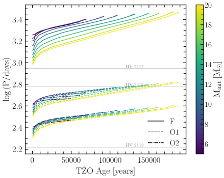
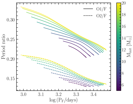
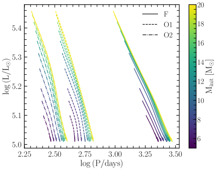
Figure 5: Pulsation properties of our TŻOs with default model assumptions. Panel a: the evolution of the pulsation period as a function of time for the fundamental (solid), first (dashed), and second overtones (dot-dashed). Panel b: Petersen diagram showing the ratio of the first overtone to the fundamental (solid), and the second to the fundamental (dashed). Panel c: The pulsation period as a function of the surface luminosity, lines have the same meaning as panel a. Colours indicate the initial mass of the TŻO. Grey dashed lines in panel a mark the observed pulsation periods of HV 2112 (Soszyński et al., 2011).

4.1 Hydrostatic pulsations

RSGs may pulsate due to the $\kappa$-mechanism in hydrogen ionisation zones, with periods between $\approx 100$–1000 days (Fox & Wood, 1982; Heger et al., 1997). Longer period pulsations may also occur, but observations can be hindered by a lack of long baseline photometry (Soraisam et al., 2018). Observations of RSG pulsations are complicated by irregular photometric variability, presumed to be caused by the interaction of large convection cells (which can have sizes of order the stellar radius) and the pulsation modes (Kiss et al., 2006).

Using the GYRE v6.0 (Townsend & Teitler, 2013; Townsend et al., 2018) stellar oscillation code, we compute the adiabatic pulsations for our TŻOs with $\rm{M_{init}}=5$–$20\,\,\rm{M}_{\odot}$ for the radial ($l=0$) modes. Figure 5 shows the time evolution of the pulsation period, Figure 5 shows a Petersen diagram (Petersen, 1973) of the period ratios, while Figure 5 shows the period-luminosity relationship.

In 5 we can see that the fundamental mode is always greater than 1000 days, and this increases with time. The first and second overtones are $\approx 500$ and $250$ days respectively. The highest-mass models start with lower periods than the low-mass models. While exploring other parameters, we find that the period of the fundamental mode is predominately sensitive to $\rm{Y_{init}}$, potentially providing a way to constrain the helium composition of a TŻO.

Figure 5 shows a Petersen diagram of the period ratios compared with the fundamental period. We can see that in general the period ratio is small ($\approx 0.2$–0.3), decreases as the period increases (and thus decreases with time), as well as decreasing with initial mass. OGLE observations of the SMC and LMC (Soszyński et al., 2004), show most objects with $\log(\rm{P/days})>3$, have period ratios $\approx 0.1$. Therefore our TŻOs exist in a region of parameter space distinct from most other objects, potentially providing an easy method to search for TŻO candidates.

Finally, Figure 5 shows the period-luminosity relationship for our TŻOs. We can see a tight relationship between their pulsation period and luminosity. Thus TŻOs may prove useful for determining distances if they can be detected and identified.

HV 2112 has a measured set of pulsation periods from OGLE of 165.59, 604.4, and 887.3 days (Soszyński et al., 2011). From Figure 5 it is difficult to match the models to the measured periods of HV 2112. To match the 604.4 and 887.3 day periods will require the first and second overtones to increase their periods by a factor of $\approx 2$.

Variations in other model parameters (Appendix A) lead to changes in the predicted pulsation periods. However, no parameter variation we have tested is able to fit the measured periods of HV 2112, over the time we have evolved our TŻOs for (though our grid is not exhaustive). The pulsation periods are predominately set by the initial mass, the mass of the NS, $\rm{\alpha_{mlt}}$, and the initial helium fraction, while not being sensitive to the initial metallicity. The fundamental mode is most strongly affected by $\rm{Y_{init}}$, with $\rm{Y_{init}}$=0.65 able to have $P>10^{5}$ days, while the first overtone is more strongly affected by $\rm{\alpha_{mlt}}$.

The closest match in our (non-comprehensive) grid is from the 5$\,\rm{M}_{\odot}$ TŻO with $\rm{\alpha_{mlt}}=3.0$, with a first overtone period of $\approx 750$ days. Based on 3D models values of $\rm{\alpha_{mlt}}=3$–4 have been proposed for RSG envelopes (Goldberg et al., 2022). We speculate a slightly more massive TŻO with a relatively high $\rm{\alpha_{mlt}}$ would be able to better fit the pulsation periods of HV 2112. If HV 2112 were a TŻO with a high $\rm{\alpha_{mlt}}$, then we would predict that we have observed the first, second, and third overtones, and that the fundamental mode is currently undetected with a period in the 1500–3000 day range.

VX Sgr has a measured pulsation period of 757 days, with a possible longer period at 28,279 days (Tabernero et al., 2021). Though Tabernero et al. (2021) caution the 28,279 days is comparable to the total time span that VX Sgr has been observed for, and thus may be an artifact of the observing period. There are also a number of shorter pulsations that vary in period and amplitude, around $~{}600$ days. The lack of a detected period between 1000-3000 days rules out most of our TŻO models. The only models that can match the 28,279 day period (assuming that it is real), is our most helium enriched model with $\rm{Y_{init}}=0.65$. This model has a fundamental mode that increase with age and can be between $P\approx 10^{3}$–$10^{5}$ days. Thus if VX Sgr where a TŻO it would imply the merger occurred with an evolved star after significant amounts of helium had been produced in the companion.

HV 11417 has measured pulsation periods of 214, 793, and 1092 days (Soszyński et al., 2009, 2011). Based on Figure 5, the 1092 day period would imply it was a very young ($\lesssim 2000$ year) and massive ($\sim 20\,\rm{M}_{\odot}$) TŻO. However models in this mass and age range would be inconsistent with the reported luminosity of HV 11417 by $\sim 0.6$ dex. Thus we conclude HV 11417 is inconsistent with our a TŻO models.

4.2 Oscillations in the nuclear burning rate

Figure 6 shows the total nuclear energy integrated over our default 5$\,\rm{M}_{\odot}$ TŻO for the $\rm{\mathrm{{}^{12}C}(p,\gamma)\mathrm{{}^{13}N}}$ and $\rm{\mathrm{{}^{14}N}(p,\gamma)\mathrm{{}^{15}O}}$ reactions. These two rates constitute  85% of the nuclear energy generated in our models (with the approx21.net) network. As the approx21.net network approximates CNO burning, $\rm{\mathrm{{}^{12}C}(p,\gamma)\mathrm{{}^{13}N}}$ is a proxy for the chain $\rm{\mathrm{{}^{12}C}(p,\gamma)\mathrm{{}^{13}N}(,e^{+}\nu)\mathrm{{}^{13}C}(p,\gamma)\mathrm{{}^{14}N}}$, while $\rm{\mathrm{{}^{14}N}(p,\gamma)\mathrm{{}^{15}O}}$ proxies the chain $\rm{\mathrm{{}^{14}N}(p,\gamma)\mathrm{{}^{15}O}(,e^{+}\nu)\mathrm{{}^{15}N}}$.

When the TŻOs are $\lesssim 24,000$ years old the variations in the reaction rates are small and approximately the size of the linewidth in Figure 6. Once the TŻO reaches $\approx 24,000$ years the reaction rates begin showing a medium level variability, with a short period variability of a few years embedded in a longer $\approx 100$ year period cycle (which is shown in the insert). This leads to a variation in the surface luminosity of $\Delta\rm{\log\left(L/L_{\odot}\right)}\approx 0.001$ dex. Then when the TŻO reaches $\approx 50,000$ years, the model undergoes large variations in the reaction rates. The energy generation rate increases by a factor $\approx 15$ to $\approx 10^{38}\,\rm{erg/s}$ and the surface luminosity can vary by $\Delta\rm{\log\left(L/L_{\odot}\right)}\approx 0.5$ dex. This is when we can no longer follow the evolution with hydrodynamics included in the model,

We can locally suppress the hydrodynamics in the envelope by using velocity_logt_lower_bound=5, which turns off the hydrodynamics in zones where the local temperature is $\rm{\log\left(T_{eff}/K\right)}<5.0$ which allows the evolution to continue for another $\approx 40,000$ years. As the TŻO evolves at this point the nuclear energy generation rates drops, returning to its pre-large amplitude burning values, before once again becoming numerically unstable and the evolution ceases.

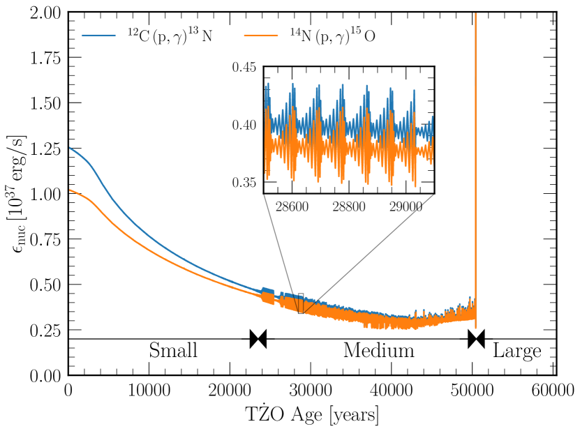
Figure 6: The nuclear energy released, integrated over the TŻO for the two most energetic reactions in our default 5$\,\rm{M}_{\odot}$ TŻO evolved with the approx21.net. These two reactions provide $\approx 85\%$ of the star’s nuclear energy. The inset shows a zoom-in where the reaction rates begin to undergo medium oscillations. These oscillations are still within the TŻO’s hydrostatic phase of evolution. At $\approx 50,000$ years the nuclear energy generation rate increases rapidly and exceeds the plot limits while becoming hydrodynamic. Text labels denote the approximate boundaries between the different amplitudes of the pulsations.

4.3 Hydrodynamic pulsations

Convective envelopes are known to be able to have dynamical instabilities that can lead to mass loss (Paczyński, 1969; Tuchman et al., 1978, 1979). Given a suitable excitation these dynamical instabilities can lead to mass loss rates of $\sim 10^{-3}\rm{M}_{\odot}\,\rm{yr}^{-1}$ through pulsational mass loss events (Clayton et al., 2017). Here we show what happens to our TŻOs as they undergo RSG pulsations.

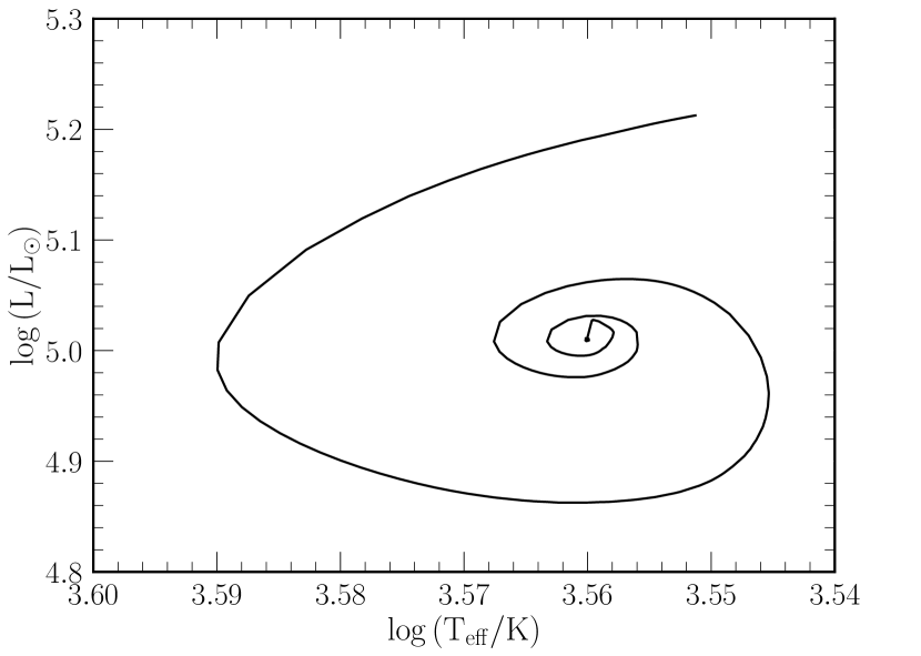
Figure 7: The surface temperature and luminosity for a our default 5$\,\rm{M}_{\odot}$ TŻO during the dynamical pulsations. This plot shows $\approx 180$ years of evolution.

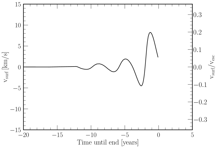
Figure 8: The radial velocity of the surface layers of our $5\,\rm{M}_{\odot}{}$ default TŻO over time. The right-hand axis shows the approximate fraction of the escape velocity that the material reaches. The x-axis is the time until we can no longer follow the evolution with MESA.

Figure 7 shows the HRD of our 5$\,\rm{M}_{\odot}$ default TŻO during this dynamical phase. Note this is only a representative plot, the exact shape of the spiral and number of cycles we can follow depends sensitively on the input physics and numerical resolution. We can see that as the star evolves the change in surface temperature and luminosity increases with each additional cycle.

Figure 8 shows the radial velocity of the surface layers of our default 5$\,\rm{M}_{\odot}$ TŻO. As the TŻO evolves the surface layers can reach velocities of $\approx\,10\,{\mathrm{km\ s^{-1}}}$, and during the final contraction phase becomes supersonic. These velocities are of a similar magnitude to those found in Yoon & Cantiello (2010) for the evolution of massive stars with pulsation-driven superwinds. This suggests that we should expect pulsation-driven mass loss in a TŻO. Yoon & Cantiello (2010) finds the mass loss rate may increase up to $10^{-2}\,\rm{M}_{\odot}\,\rm{yr}^{-1}$. These RSG pulsations are resolved when the timestep of our models drops significantly below the pulsation period. This occurs in our TŻOs when the nuclear burning rate spikes, as seen in Figure 6, but can occur at earlier times if we artificially enforce a short timestep. If the mass loss rates are at the upper end of those predicted by Yoon & Cantiello (2010) then this implies a lifetime of $\approx$ 100–1000 years. However, our wind mass loss is based on that of van Loon et al. (2005) which is based on the observations of RSG’s and thus has this mass-loss built into the time averaged mass-loss rates. More work is needed to understand the wind/pulsational mass loss rates in RSG’s, as this will set the lifetime of a TŻO.

5 Nucleosynthesis

Figure 9 shows the surface composition relative to the initial composition for TŻOs evolved with a fully coupled 399 isotope nuclear network at $\approx 10,000$ years after formation. Figure 9(a) shows the composition as $\rm{Y_{init}}$ is varied, for a fixed $\rm{M_{init}}=5\,\rm{M}_{\odot}$ and $\rm{Z_{init}}=10^{-4}$. Figure 9(b) shows the composition as $\rm{M_{init}}$ is varied for fixed $\rm{Y_{init}}=0.28$ and $\rm{Z_{init}}=10^{-3}$. A HRD for the models in Figure 9(a) can be found in Appendix A. We include all isotopes produced in our models, without taking into account any radioactive decay. A comparison with the results of C93 can be found in Appendix B. We note, as a word of caution, that this abundance pattern is sensitive to the choice of the initial composition, as the initial metals act as seed nuclei for the rp-burning.

For the $\rm{Z_{init}}=10^{-4}$ we find that for $Z<20$, there is no enhancement relative to the initial composition. For $21\leq Z\leq 25$ (Sc to Mn) there is an enhancement that increases as $\rm{Y_{init}}$ increases, while both Fe and Ca are not enhanced. For higher atomic numbers the enhancement relative to the starting composition becomes larger, up to $\approx 10^{5}$ their starting values. As $\rm{Y_{init}}$ increases the most enhanced element decreases in atomic number, for $\rm{Y_{init}}=0.28$ it is Br, $\rm{Y_{init}}=0.4$ it is As, and $\rm{Y_{init}}=0.6$ it is Ga. After this peak element, there is a rapid decline in the production of heavier elements. Mo is only enhanced in our $\rm{Y_{init}}$=0.28 model and is thus not a good element for determining a TŻO status.

These differences are due to the knee temperature decreasing as $\rm{Y_{init}}$ increases. This lowers the maximum mass of an element that can be produced in the irp-process. We reconfirm the previous findings of Biehle (1991) and show that we can have significant enhancement of the elements Rb, Sr, Y, Zr and Mo but this depends sensitivity on the initial He composition. We find that models with very high initial helium fractions can lack Rb. Thus there could be a population of helium-rich TŻOs without Rb, possibly explaining the difficulty in confirming the detection of a TŻO with the Rb mass fractions alone.

For the $\rm{Z_{init}}=10^{-3}$ models we see almost no enhancement of metals at all. There is a slight enhancement of N due to CNO burning as well as an enhancement of S–Ar for the $\rm{M_{init}}=5\,\rm{M}_{\odot}$ model, and enhancements in Ca–Mn for the $\rm{M_{init}}=10\,\rm{M}_{\odot}$ and $15\,\rm{M}_{\odot}$ models. However there is no production of elements with $Z>25$. This is due to the higher opacity at the knee, lowering the knee luminosity, which lowers the knee temperature. Thus, at metallicities comparable to the SMC, LMC, or MW, TŻOs are unlikely to be distinguishable from non-TŻO stars based on their surface composition alone of elements such as Rb or Mo.

Table 1 shows the surface mass-fraction ratios for a selected set of elements for the $\rm{Z_{init}}=10^{-4}$ models. Also shown is a comparison with Model A of C93. We can see that the estimates for Ni/Fe are similar for all initial helium fractions. Estimates for Rb/Ni and Rb/Fe depend on the initial helium fraction but can be consistent with C93 for $0.28<\rm{Y_{init}}<0.4$ (C93 assumes $\rm{Y_{init}}$=0.32). Finally, Mo/Fe is extremely different, with our models predicting very little absolute Mo, with the valued decreasing as $\rm{Y_{init}}$ increases. Other ratios including K/Ca and Ca/Fe are a factor 10 smaller than C93.

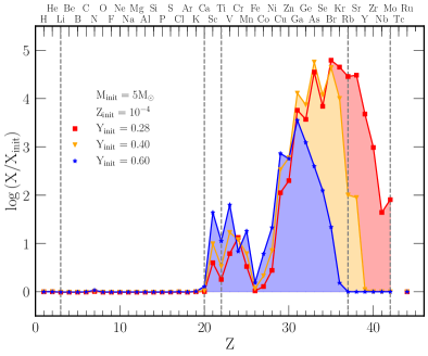
(a) Variations in $\rm{Y_{init}}$

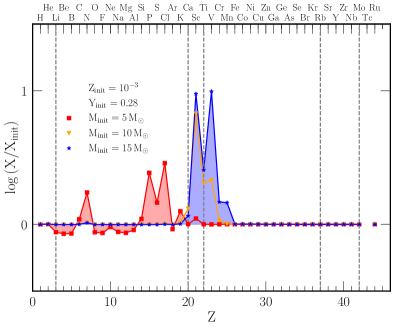
(b) Variations in $\rm{M_{init}}$

Figure 9: The surface composition relative to the initial composition at 10,000 years post-TŻO formation. Left panel: The composition as a function of of the proton number Z for a 5$\,\rm{M}_{\odot}$ TŻO and $\rm{Z_{init}}=10^{-4}$ with $\rm{Y_{init}}=0.28$ (red square), $\rm{Y_{init}}=0.4$ (orange triangle), $\rm{Y_{init}}=0.6$ (blue star). Right panel: The composition as a function of of the proton number Z for $\rm{Y_{init}}=0.28$ and $\rm{Z_{init}}=10^{-3}$, with $\rm{M_{init}}=5\,\rm{M}_{\odot}{}$ (red square), $\rm{M_{init}}=10\,\rm{M}_{\odot}{}$ (orange triangle), and $\rm{M_{init}}=15\,\rm{M}_{\odot}{}$ (blue star). All models were evolved with a fully coupled 399 isotope nuclear network. Vertical lines mark elements that may be useful for detecting TŻOs. Note the change in the y-scale between panels. Data tables are available in the online Zenodo material with the time evolution of the composition.

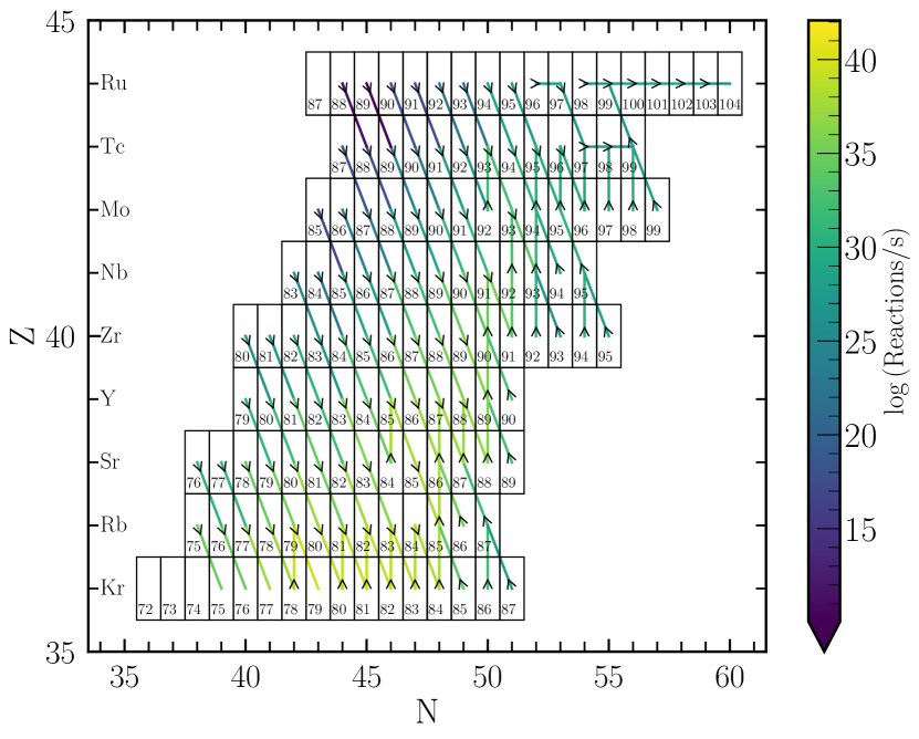
Figure 10: The total isotopic flow rate due to nuclear reactions for a selected set of isotopes in our default 5$\,\rm{M}_{\odot}$ TŻO evolved with an 399 isotope nuclear network. The coloured lines show the logarithm of the net number of reactions per second for each isotope, showing only the most significant reaction, taking into account both forward and reverse reactions and summed over the entire TŻO. Arrows show the direction of flow. The model shown is $\approx 10,000$ years post-TŻO formation. Isotopes with no arrows have total reaction rates less than the lower limit of $10^{10}$ reactions/s. The atomic mass is quoted for each isotope in each box.

Figure 10 shows how the isotopic composition will change over time, by showing the reaction flow for the dominant reaction for each isotope. Diagonal lines to the lower right are due to beta decays. There are insufficient free neutrons for the $(n,p)$ reactions to dominate as both $\mathrm{{}^{13}C}$ and $\mathrm{{}^{22}Ne}$ have mass fractions $X\lesssim 10^{-17}$ at the base of the envelope. Vertical lines indicate a proton capture, while horizontal lines denote neutron captures. $\alpha$-captures are included in the network but are rarely significant in this mass range. Isotopes with no lines are included in the network but have all their reaction rates $<10^{10}$ reactions/s.

Isotopes are predominately decaying via beta-decays faster than proton captures can increase the atomic number of the isotope. Thus the flow is towards more neutron-rich isotopes, rather than more proton-rich isotopes. This prevents significant rp-burning from occurring and causes the limited amount of Mo shown in Figure 9(a). The maximum atomic number that is reached, before beta-decays outpace the proton captures will depend on the peak temperature reached by the TŻO at the base of the convection zone (Fisker et al., 2008). Thus, given Figure 2, the peak atomic number reached depends on the initial mass as well.

We have tested our choice of nuclear network in Appendix B. Changing our nuclear network to one that closely matches that of C93, has little effect on the results (see Appendix B). Though by extending to higher atomic numbers we can see a similar turn over in the mass fraction pattern in C93 as we see, except for C93 this occurs at higher atomic numbers.

Element	$\rm{Y_{init}}=0.28$	$\rm{Y_{init}}=0.40$	$\rm{Y_{init}}=0.60$	C93
ratio				Model A
Rb/Ni	2.18E+00	3.00E-03	9.94E-06	1.82E-01
Rb/Fe	3.38E-01	1.07E-03	8.04E-06	1.48E-01
Li/Ca	1.55E-04	1.49E-04	1.23E-04
Li/K	2.67E-03	2.67E-03	2.64E-03
Mo/Fe	3.99E-04	4.44E-06	3.36E-06	1.23E-01
Ni/Fe	1.55E-01	3.57E-01	8.08E-01	8.13E-01
K/Ca	5.80E-02	5.59E-02	4.64E-02	1.58E-01
Ca/Fe	4.91E-02	4.58E-02	4.23E-02	8.91E-01
Rb/Zr	1.76E+01	5.99E+01	5.97E-01	4.17E+00

Table 1: Ratio of surface mass fractions for selected elements for our 5$\,\rm{M}_{\odot}$ TŻOs, evolved with the large 399 isotope nuclear network, at 10,000 years after TŻO formation at $\rm{Z_{init}}=10^{-4}$. The final column contains the Model A data from C93 which only provides mass fractions for Carbon and heavier elements and thus lacks Lithium for comparison with.

Neutrino losses from our TŻOs are $\approx 10^{37}\rm{erg/s}$. This is dominated by the losses due to beta-decays, while the thermal neutrino losses are negligible. This is only a lower limit on the neutrino flux, as there may be additional neutrino emissions from the material below the knee which we do not model. This neutrino flux is comparable to a solar-mass star at the tip of the red giant branch (Farag et al., 2020), and is unlikely to be detectable with current detectors (Patton et al., 2017a; Patton et al., 2017b).

5.1 ${}^{44}\rm{Ti}\rm{O}_{2}$ and ${}^{44}\rm{Ti}\rm{O}$

While the predicted unique nucleosynthetic signal of a TŻO has been used previously to make claims for the detection (or not) of a TŻO, it is not without controversy (Tout et al., 2014). Thus we propose a new signal which provides a more constraining nucleosynthetic signal, namely the detection of molecules of TiO₂ and TiO containing the radioactive isotope $\mathrm{{}^{44}Ti}$.

$\mathrm{{}^{44}Ti}$ has a half life of $\approx 60$ years (Audi et al., 2003; Ahmad et al., 2006) and is usually found in the ejecta of core-collapse supernovae (Iyudin et al., 1994). Typical core-collapse supernovae have ejecta of $10^{-5}$–$10^{-4}\,\,\rm{M}_{\odot}$ of $\mathrm{{}^{44}Ti}$ rich material (Magkotsios et al., 2010). This suggests that the detection of $\mathrm{{}^{44}Ti}$ in a TŻO could be the result of contamination from the supernovae that formed the NS initially. However, given its short half-life, unless we detect a TŻO shortly after the birth of the NS (when the SN remnant should still be visible) then the detection of $\mathrm{{}^{44}Ti}$ requires a continuous production site.

In non-TŻO stars, $\mathrm{{}^{44}Ti}$ is normally produced deep in the stellar core, via $\mathrm{{}^{40}Ca}(\alpha,\gamma)\mathrm{{}^{44}Ti}$ during the late stages of stellar evolution and during explosive burning episodes (Timmes et al., 1996). Coupled with this, is that we need to be able to efficiently mix the $\mathrm{{}^{44}Ti}$ to the surface of the star, which is difficult to achieve unless the convective envelope penetrates deep into the core which is unexpected when $\mathrm{{}^{40}Ca}(\alpha,\gamma)\mathrm{{}^{44}Ti}$ is active.

For reference we computed a $\rm{M_{init}}=5\,\rm{M}_{\odot}$ AGB star, $\rm{M_{init}}=8\,\rm{M}_{\odot}$ SAGB star and $\rm{M_{init}}=10\,\rm{M}_{\odot}$ massive star with $\rm{Z_{init}}=0.00142$ ($\sim Z_{\odot}/10$). For computational reasons we used a truncated version of our 399 isotope nuclear network. We took our 399 network and removed all elements heavier than Fe, as we are only interested in the Ti isotopes, which brings the total isotope count down to 172.

The 5$\,\rm{M}_{\odot}$ model is evolved until $\approx 40$ thermal pulses while the 8 and $10\,\rm{M}_{\odot}$ models are evolved up to carbon ignition. We find the maximum surface mass fraction of $\mathrm{{}^{44}Ti}$/$\mathrm{{}^{48}Ti}$ remains effectively zero (and always lower than the numerical tolerance imposed on the nuclear network solver) throughout the evolution.

However, distinguishing different isotopes directly in a spectrum can be challenging. Thus we propose looking for isotopologues of $\rm{Ti}\rm{O}_{2}$ and $\rm{Ti}\rm{O}$. Our TŻOs almost always have surface temperatures $\log\ (T_{\rm eff}/K)<3.6$, where $\rm{Ti}\rm{O}_{2}$ and $\rm{Ti}\rm{O}$ molecules are expected to form (Pavlenko et al., 2020), thus there should be a significant amount of $\rm{Ti}\rm{O}_{2}$ and $\rm{Ti}\rm{O}$ in the atmospheres of the TŻOs.

The most common Ti isotope is $\mathrm{{}^{48}Ti}$, with contributions from $\mathrm{{}^{46-50}Ti}$ (Asplund et al., 2009). Detecting the different isotopologues has been achieved for these isotopes, due to a shift in the molecular lines as the mass of the molecules $\rm{Ti}\rm{O}_{2}$ and $\rm{Ti}\rm{O}$ change with the different isotopic compositions (Breier et al., 2019). The size of this shift is relative to the change in the molecular mass between the isotopologues (Herzberg, 1950). Thus a molecule containing $\mathrm{{}^{44}Ti}$ will have a larger shift in its molecular lines than the already detectable isotopologues containing $\mathrm{{}^{46-50}Ti}$ (Pavlenko et al., 2020; Serindag et al., 2021). It may also be possible to use millimetre/submillimetre observations to detect $\mathrm{{}^{44}Ti}\rm{O}$ given the detection of other TiO isotopologues (Kamiński et al., 2013; Lincowski et al., 2016).

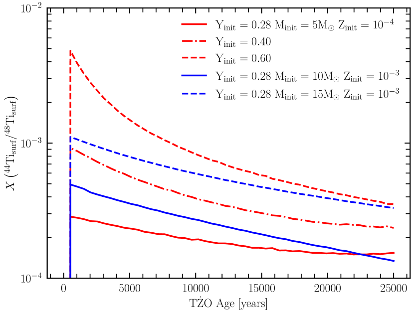
Figure 11: The ratio of the surface mass fraction of $\mathrm{{}^{44}Ti}$ to surface $\mathrm{{}^{48}Ti}$ over the TŻOs lifetime. In blue models with $\rm{M_{init}}=5\,\rm{M}_{\odot}$, and $\rm{Z_{init}}=10^{-4}$ where solid line has $\rm{Y_{init}}=0.28$, dot-dashed $\rm{Y_{init}}=0.4$, and dashed $\rm{Y_{init}}=0.6$. In green models with $\rm{Z_{init}}=10^{-3}$ and $\rm{Y_{init}}=0.28$, where the sold line has $\rm{M_{init}}=10\,\rm{M}_{\odot}$, and dashed has $\rm{M_{init}}=15\,\rm{M}_{\odot}$. Models were stopped at $\approx 25,000$ years.

In our TŻO models $\mathrm{{}^{44}Ti}$ is produced in the CaScTi cycle via $\mathrm{{}^{43}Sc}\left(p,\gamma\right)\mathrm{{}^{44}Ti}$ (Fisker et al., 2008). The $\mathrm{{}^{44}Ti}$ is then mixed outwards before it can capture another proton. Figure 11 shows the surface mass fraction of $\mathrm{{}^{44}Ti}$/$\mathrm{{}^{48}Ti}$. Depending on $\rm{Y_{init}}$, $\rm{Z_{init}}$, and $\rm{M_{init}}$ the ratios starts between $10^{-4}$–$10^{-2}$ and decreases with time. On long timescales, we can see that the ratio tends towards $X(\mathrm{{}^{44}Ti}/\mathrm{{}^{48}Ti})\approx 10^{-4}$. This is due to increasing amounts of $\mathrm{{}^{48}Ti}$ (other stable Ti isotopes are also increasing with time), while the absolute amount of $\mathrm{{}^{44}Ti}$ remains approximately constant. For the TŻOs with $\rm{Z_{init}}=10^{-3}$ the ratio decreases with $\rm{M_{init}}$. A 5$\,\rm{M}_{\odot}$ TŻO with $\rm{Z_{init}}=10^{-3}$ did not show any enrichment of $\mathrm{{}^{44}Ti}$. These ratio’s are much greater than the values found for the 5, 8, and 10$\,\rm{M}_{\odot}$ non-TŻO stars.

$\rm{M_{init}}$	$\rm{Y_{init}}$	$\rm{Z_{init}}$	$\mathrm{{}^{44}Ti}$	$\mathrm{{}^{46}Ti}$	$\mathrm{{}^{47}Ti}$	$\mathrm{{}^{48}Ti}$	$\mathrm{{}^{49}Ti}$	$\mathrm{{}^{50}Ti}$
5	0.28	$10^{-4}$	3.85E-12	2.10E-09	2.76E-09	2.02E-08	6.50E-09	9.71E-10
5	0.40	$10^{-4}$	8.39E-11	1.03E-08	2.12E-08	1.01E-07	6.88E-08	9.96E-10
5	0.60	$10^{-4}$	1.31E-11	3.38E-09	5.66E-09	3.35E-08	1.71E-08	9.77E-10
5	0.28	$10^{-3}$	5.56E-16	1.43E-08	1.32E-08	1.34E-07	1.00E-08	9.86E-09
10	0.28	$10^{-3}$	5.46E-11	4.45E-08	4.57E-08	2.02E-07	6.47E-08	1.07E-08
15	0.28	$10^{-3}$	1.51E-10	3.96E-08	4.95E-08	2.55E-07	1.08E-07	1.02E-08
Sun				2.23E-07	2.08E-07	2.15E-06	1.64E-07	1.64E-07
5		$Z_{\odot}/10$	3.05E-26	2.02E-08	1.85E-08	1.88E-07	1.44E-08	1.39E-08
8		$Z_{\odot}/10$	2.16E-98	2.05E-08	1.89E-08	1.91E-07	1.43E-08	1.41E-08
10		$Z_{\odot}/10$	2.57E-98	2.05E-08	1.89E-08	1.91E-07	1.43E-08	1.41E-08

Table 2: Surface mass fractions for different Ti isotopes for our large nuclear network models. The composition is taken at $\approx 10,000$ years post TŻO formation. The 5, 8, and 10$\,\rm{M}_{\odot}$ non-TŻO stars are measured at the time of maximum surface $\mathrm{{}^{44}Ti}$. Solar values from Grevesse & Sauval (1998).

Table 2 shows the absolute mass fraction fractions of the Ti isotopes in our large nuclear network models. We can see that the amount of all Ti isotopes slightly increases with increasing initial helium fraction. There is however a factor $\sim 10$ increase in $\mathrm{{}^{44}Ti}$ as $\rm{Y_{init}}$ increases. Given the small absolute mass of $\mathrm{{}^{44}Ti}$, which is much less than that typically seen in supernovae ejecta (Magkotsios et al., 2010), it may be difficult to directly detect the gamma-ray from the decay of $\mathrm{{}^{44}Ti}$.

We note though that before this becomes a viable method it is likely we will need improved theoretical models of the molecular lines of $\mathrm{{}^{44}Ti}\rm{O}_{2}$ and $\mathrm{{}^{44}Ti}\rm{O}$, as to date experiments have concentrated on the more common and stable isotopes of titanium, namely 46–50 (Brünken et al., 2008; Breier et al., 2019; McKemmish et al., 2019; Witsch et al., 2021).

6 Suitability of model assumptions

(a) Central density

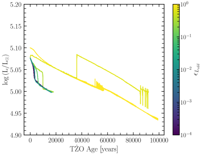
(b) Central luminosity

Figure 12: Panel a: The evolution of the surface luminosity as a function of the assumed average core density. Light colours denote higher core densities and smaller assumed NS radii. Panel b: The evolution of the surface luminosity as a function of the efficiency factor $\epsilon_{L}$. Light colours denote higher efficiencies and thus the energy injected into the inner boundary is closer to $L_{\rm Edd}$. Evolution was arbitrarily stopped when either the model reached 100,000 years, 100,000 timesteps, or when MESA could no longer follow the evolution.

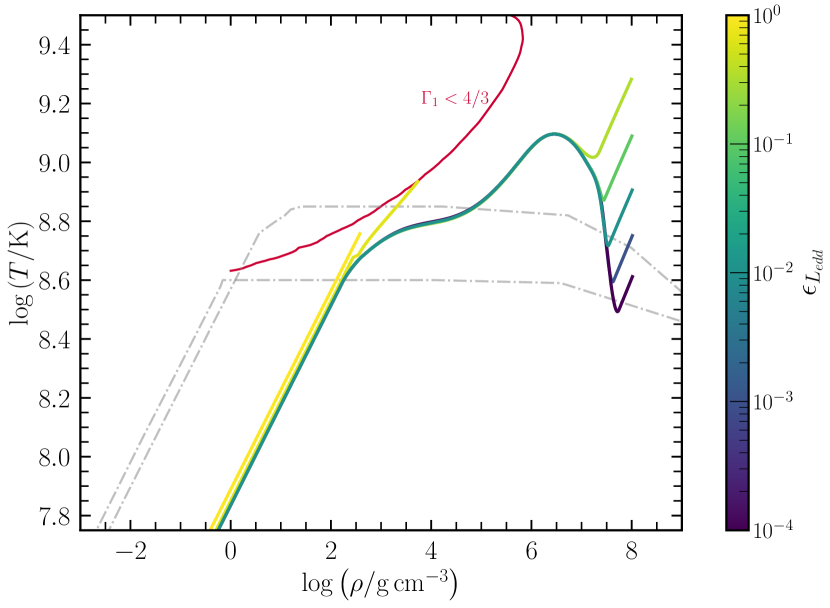
Figure 13: Top Panel: The temperature-density (T-$\rho$) profile for the models shown in Figure 12(b) at a time $\approx 10,000$ years post TŻO formation. The $\epsilon_{L}=0$ model did not reach 10,000 years and is thus not shown. Dash-dotted lines are the models of C92 while the red region is the pair-instability region.

The models presented in this work depend on two key approximations, that make the TŻO models computationally feasible. Without these approximations, these models would not be computationally viable. Both approximations deal with the fact that we can not model down to the surface of the NS while simultaneously including the RSG envelope. First, we assume a $\log\ \langle\rho_{c}/\mathrm{g}\,{\mathrm{c}\mathrm{m}}^{-3}\rangle=9.3$, which implies an effective $\rm{R_{NS}}\approx 600\,\mathrm{k}\mathrm{m}$ and secondly we inject additional energy at the base of our models. We will now test those assumptions, as far as possible, to determine their effect on our results. For this test, we turn off the hydrodynamics, as it can cause numerical convergence issues.

Figure 12 shows the total luminosity of the TŻO as a function of the age since formation, for variations in the core density (12(a)), and the injected energy (12(b)). Firstly we can see that both sets of models evolve to lower luminosities over time. Figure 12(a) compares models with $\log\langle\rho_{c}/\mathrm{g}\,{\mathrm{c}\mathrm{m}}^{-3}\rangle$ between $10^{9}$–$10^{12}\,\mathrm{g}\,{\mathrm{c}\mathrm{m}}^{-3}$ (this equates to effective NS radii between $\approx 90$–$900\,\mathrm{k}\mathrm{m}$). It shows that as the core density increases the total luminosity increases. This is due to a lower opacity at the knee, causing $L_{\rm{knee}}$ to increase. Figure 12(b) also shows that as the injected energy decreases, the surface luminosity also decreases. Thus, surprisingly, over the range of parameters explored here, the two approximations act with different signs but similar magnitudes, in terms of the total luminosity. Therefore they approximately cancel out. Comparing the surface metal mass fraction, the low $\epsilon_{L}$ models converge to values about a factor 2 greater than the $\epsilon_{L}=1$, while the highest core density models have a factor 2 lower surface metal mass fractions. Again, our two assumptions are approximately cancelling each other out.

The large luminosity jumps leading to the models then evolving on a different luminosity track are due to the lack of hydrodynamics. In models with hydrodynamics included, those jumps occur at the time when the energy generated by nuclear burning spikes and the models would normally have been stopped due to large amplitude surface pulsations being resolved in the models.

In Figure 13 we show the temperature-density profiles inside the TŻOs as a function of $\epsilon_{L}$. As $\epsilon_{L}$ decreases, less energy is injected into the model, therefore the TŻO must provide more of the energy itself. As the mass of the NS varies little in our models this is also equivalent to changing the opacity of the material at the base of the convection zone. The material below the knee then moves to higher temperatures and densities to provide the necessary energy via nuclear burning and mass accretion to support the star. The region below the knee does not evolve at a constant temperature, as previously found in Thorne & Zytkow (1975, 1977) and C92. Instead as the temperature increases, the material avoids the pair-instability region by evolving around the instability region. The T–$\rho$ tracks converge for $\epsilon_{L}\leq 0.1$, until $\log(\rho/\mathrm{g}\,{\mathrm{c}\mathrm{m}}^{-3})\approx 6.0$.

At $\log(\rho/\mathrm{g}\,{\mathrm{c}\mathrm{m}}^{-3})\approx 6.0$ the core begins evolving to cooler temperatures. At this temperature both hydrogen and helium are depleted in the material below the knee. With a very low mass fraction of carbon and oxygen, due to the low initial metallicity, and our use of the approx21.net nuclear network, the nuclear energy generation rate goes to 0 as there are no available nuclear reactions. The inner regions then begin to cool due to an increase in thermal neutrino losses as the density increases.

Finally, the increase in temperature at $\log(\rho/\mathrm{g}\,{\mathrm{c}\mathrm{m}}^{-3})\approx 8.0$ is due to a new convection zone setting in near the inner boundary of the model. This is due to the (small) amount of energy that is still being injected into the model. Models with less injected energy cool further and reach higher densities before showing this uptick.

7 Final fate

Once the large amplitude surface pulsations begin the computational timescale decreases and we begin evolving the models on the pulsation timescale. This leads to timesteps of order $10^{2}$–$10^{3}$ seconds, which is much smaller than the $10^{8}$ seconds we take during the normal phase of a TŻOs evolution and thus is infeasible to evolve over longer time frames. Numerical convergence issues also occur as shocks form in the outer envelope, preventing the models from being evolved for more than a few tens of years at this point.

Thus we can only speculate what happens next. The TŻOs are undergoing large pulsations, and in other $\epsilon$-mechanism pulsators this is expected to lead to pulsation-driven mass loss (Baraffe et al., 2001; Nakauchi et al., 2020) or, as in normal RSGs, pulsations may lead to pulsational driven superwinds (Yoon & Cantiello, 2010). This could rapidly decrease the envelope mass over $\approx 100$ years, leaving behind a bare NS. Or perhaps the TŻO will undergo a neutrino runaway when nuclear burning ceases and energy losses from neutrinos cause the TŻO to collapse (Podsiadlowski et al., 1995), leaving a BH behind, though this seems less likely as our models avoid the pair-instability region.

If the envelope was entirely ejected from the NS, it seems unlikely that the NS mass will have increased significantly enough to be visible as a higher mass NS. The accretion rate onto the NS is $\approx 10^{-9}$–$10^{-8}\,\rm{M}_{\odot}\,\rm{yr}^{-1}$. In our models, this leads to the NS gaining at most $\approx 0.002\,\,\rm{M}_{\odot}$ during its evolution. The NS may also be spun down by braking between the NS’s magnetic field and the envelope (Liu et al., 2015). In this scenario the NS will become a slow spinning NS inside a slow moving CSM that appears like a supernovae remnant, that has been proposed for RCW 103 (Liu et al., 2015).

The other option is that the TŻO runs out of CNO material, which provides the bulk of the nuclear energy generated (Biehle, 1994). In this case, the envelope may collapse onto the NS forming a BH, possibly leading to a transient event (Moriya, 2018; Moriya & Blinnikov, 2021). In a 5$\,\rm{M}_{\odot}$ TŻO model the total mass of CNO elements decreases at a rate of $\approx 10^{-10}\,\rm{M}_{\odot}\,\rm{yr}^{-1}$. With an initial mass of $\approx 10^{-5}\,\,\rm{M}_{\odot}$ of CNO elements (for $\rm{Z_{init}}=10^{-5}$), this gives an upper limit of $\approx 10^{6}$ years, assuming the burn rate continues at the same rate. This is comparable to the lifetime given assuming a steady state wind mass loss.

If the NS inside the TŻO did collapse into a BH and form a transient event, this may look like a type IIn SN. The pre-SN pulsations likely removed 1–10$\,\rm{M}_{\odot}$ of material in the 100–1000 years before the final collapse. At collapse it is then likely that there is only a few solar masses, at most, of H-rich envelope left. Our default 5$\,\rm{M}_{\odot}$ TŻO has only a $\approx 2.5\,\rm{M}_{\odot}$ envelope left before the pulsations begin, while at 20$\,\rm{M}_{\odot}$ has $\approx 5.5\,\rm{M}_{\odot}$ envelope before the pulsations begin. We would not expect any significant $\mathrm{{}^{56}Ni}$ production in the event, and as the TŻO was fully mixed there would not be any observed change in the composition at late times. To power a SN transient event would require it either to be entirely powered by CSM interaction, energy released as the NS collapses into a BH, or if the BH generates a jet from additional mass accretion (Fryer et al., 1996; Qin et al., 1998; Fryer et al., 2014).

8 Discussion

In this work, we have been agnostic as to how a TŻO formed, whether it was a direct impact, common envelope merger, or dynamical merger. Each of the formation pathways may impact the resulting TŻO. Common-envelope mergers require that the companion star is evolved, with a helium-rich core and an envelope that is increasing in radius. While direct impacts and dynamical mergers are less sensitive to the companion star’s evolutionary state, at least regarding when a merger can occur. Merging at different points in the star’s pre-TŻO life will lead to a different initial metal fraction than our assumed solar-scaled metal distribution, and limits what values of $\rm{Y_{init}}$ are possible. There could be differences in whether or not a merger results in a TŻO or instead causes enhanced mass loss, leaving behind a tight binary with an NS, thus failed TŻO’s are progenitors for double NS systems (DNS). Detections of TŻOs could place constraints on the uncertain merger rate of DNS systems as currently being probed by gravitational wave detections.

We assumed that the starting point for a TŻO can be approximated as a normal star, which then becomes fully convective. However, it is possible that the companion was the accretor in a binary system. The material it gains will be enriched by the nuclear burning in the donor (Farmer et al., 2021, 2023) and the internal structure of the accretor will be altered by the mass accretion (Renzo & Götberg, 2021; Renzo et al., 2023). This may lead to possible different outcomes during the merger, which may include additional mass loss, changes in the probability of a successful TŻO formation, and to initially enrich the TŻO in additional metals.

It was argued in C93 that it was necessary to use a two-stream convection model to follow the nucleosynthesis. Here the composition is tracked for material that is convectivly moving towards the knee and away from the knee. As material moves towards the NS it undergoes proton captures, before mixing away from the knee, where it can then undergo beta decays, before being mixed back towards the knee. As the burning timescale is comparable to the mixing timescale at the base of the envelope the chemical composition of material flowing up/down may be significantly different. MESA takes assumes a diffusion equation for chemical transport. The effect of having a diffusion model is that we likely over predict the production of heavy nuclei. In the MESA models some heavy nuclei will be able stay near the base of the envelope, where the temperatures are highest, for much longer than they would if they where being mixed outwards on a timescale similar to their burning timescale. Thus they can undergo additional proton captures and produce even heavier nuclei. This may suggest we are even less likely to see a detectable nucleosynthetic signal in TŻOs in the local Universe.

9 Conclusions

In this work, we have computed the first set of MESA TŻOs. We did this by adjusting the inner boundary of the model to approximate the NS at the centre of each TŻO. We have then followed the evolution of the TŻOs. We have also explored in detail the pulsation periods with the GYRE stellar oscillation instrument, and computed detailed nucleosynthetic signatures with a large fully-coupled 399 isotope nuclear network. Our results can be summarised as follows:

• We find that TŻOs evolve to lower luminosities and lower temperatures during their lifetime. We have also expanded the range of possible locations for TŻOs to be between $\rm{\log\left(T_{eff}/K\right)}\approx 3.47$–$3.6$ and $\rm{\log\left(L/L_{\odot}\right)}\approx 5.0$–$5.5$.

• We do not find a gap in the parameter space where models can not exist. This is because our models are denser than previously predicted, which prevents models from evolving into the pair-instability region.

• We have computed the pulsation periods of our TŻOs and find the longest periods to be $\approx 250,500$ and 1000-2000 days.

• If HV 2112 is a TŻO, we predict there should be a currently undetected 1500–3000 day pulsation period. If detected this will also imply $\rm{\alpha_{mlt}}\approx 3$ in the envelopes of TŻOs.

• If VX Sgr were a TŻO and its $\sim 28,000$ day pulsation period were real, this would imply it is a very helium enriched TŻO.

• Based on the measured pulsation periods of HV 11417 we would infer it to be a massive, but very young TŻO. However this is inconsistent with the measured luminosity of HV 11417. Thus we rule out HV 11417 as a TŻO.

• Our results and the predicted lifetimes depend strongly on the mass-loss rates due to RSG pulsations. The lifetime of the TŻO will depend on the total mass-loss rate experienced by the TŻO. If RSG pulsations remove significant amounts of material then the lifetime of a TŻO may only be 100–1000 years.

• Assuming the RSGs do not experience significantly higher mass loss than we assume, then we estimate a lifetime in the range of $10^{4}$–$10^{5}$ years. Contrary to non-TŻO stars, the higher the initial mass of the TŻO the longer it lives.

• We have computed several of our models with a large 399 isotope fully-coupled nuclear network. We reconfirm the previous findings that Rb, Sr, Y, Zr can be enhanced due to the irp-burning. However, the level of enhancement is sensitive to the initial composition of the TŻOs.

• At higher initial metallicities TŻOs do not show any metal enrichment due to a lower knee temperature, caused by the increasing opacity at the knee as the metallicity increases. Thus in the local Universe TŻOs may not be distinguishable from non-TŻOs based on their nucleosynthesis alone.

• We propose a new observational signal, that of molecules containing $\mathrm{{}^{44}Ti}$. Due to the high-temperature burning and fully convective envelope of the TŻO, $\mathrm{{}^{44}Ti}$ can be mixed to the surface before it decays. There in the cooler envelope, it can form $\mathrm{{}^{44}Ti}$O₂ and $\mathrm{{}^{44}Ti}$O, which could be detectable due to the shift in their molecular lines compared to stable Ti-containing molecules.

• TŻOs represent a class of stars that are exceptional tests of the numerical capabilities of a stellar evolution code. This work has led to many improvements and code fixes in the MESA stellar evolution code that have applications far outside that of TŻOs.

Data Availability

All input files and all output data is made available at https://doi.org/10.5281/zenodo.4534425.

Appendix A Sensitivity to other parameter choices

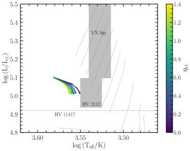
(a) Wind efficiency

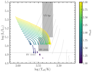
(b) Mixing Length alpha

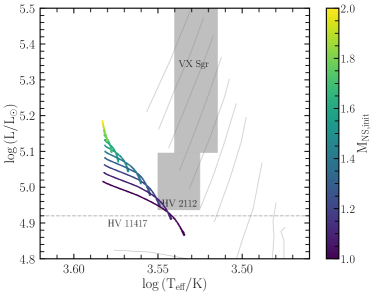
(c) Initial Mass NS

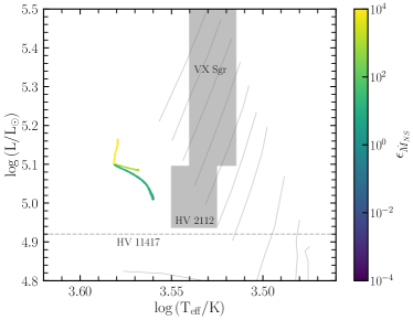
(d) NS accretion rate

Figure 14: HRDs for variations in our TŻO modelling assumptions. Grey lines and grey boxes have the same meaning as in Figure 1. All models are taken as 5$\,\rm{M}_{\odot}$ with a $M_{\rm NS}=1.4\,\,\rm{M}_{\odot}$, and use our default parameters except for those being varied in each panel. Panel a: variations in the wind mass loss efficiency, panel b: variations in the mixing length alpha, panel c: variations in the mass of the NS, and panel d: variations in the accretion rate onto the NS.

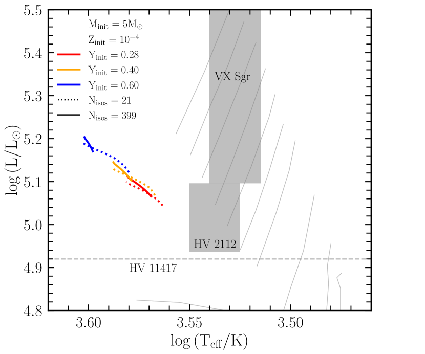
Figure 15: HRDs for variations in the size of the nuclear network. Grey lines and grey boxes have the same meaning as in Figure 1. All models are taken as 5$\,\rm{M}_{\odot}$ with a $M_{\rm NS}=1.4\,\,\rm{M}_{\odot}$, and use our default parameters. The red lines show $\rm{Y_{init}}$=0.28, the orange line shows $\rm{Y_{init}}$=0.4, and the blue lines show $\rm{Y_{init}}$=0.6 and are evolved with $\rm{Z_{init}}=10^{-4}$. Solid lines are models that are evolved with the 399 isotope network, while dotted lines show the 21 isotope network, with the same $\rm{Y_{init}}$. All models were stopped after 25,000 years.

Figure 14 shows the HRDs for the parameter variations we have tested here, while Figure 15 shows the HRD for a hydrogen-rich and helium-rich TŻO evolved with our 399 isotope network.

A.1 Wind mass loss

Figure 14(a) shows variations in the wind mass loss efficiency $\eta_{\rm{\rm VL}}$, which scales the wind mass loss rates of van Loon et al. (2005). All models start with a similar evolution, however as the mass loss rate increases TŻOs become less luminous for a given temperature. As $\eta_{\rm{\rm VL}}$ increases models stop their evolution at higher surface temperatures, live for less time overall, and enrich the surface with fewer metals (at a given age). The effect of wind mass loss on a stellar model is more complex than a single scaling factor (Renzo et al., 2017).

A.2 Mixing length alpha

Figure 14(b) shows variations in the mixing length $\rm{\alpha_{mlt}}$. As $\rm{\alpha_{mlt}}$ increases the tracks are more luminous and hotter, acting like a more massive TŻO (See Figure 1). This increase in luminosity is due to the knee temperature increasing with increasing $\rm{\alpha_{mlt}}$. Models with $\rm{\alpha_{mlt}}<1.5$ act similar to the high metallicity models in Section 3.1. That is, they have a high opacity at the knee, which leads to a low $L_{\rm{knee}}$, and thus a low knee temperature. As $\rm{\alpha_{mlt}}$ increases, TŻOs produce more metals (at a given age). The age of the TŻO is approximately independent of the assumed $\rm{\alpha_{mlt}}$.

A.3 Core mass

Figure 14(c) shows variations in the neutron star mass $M_{\rm NS}$. As $M_{\rm NS}$ increases stars are more luminous, though at a similar surface temperature. As the TŻO evolves, low mass NSs have both a larger change in luminosity and a drop to a lower final luminosity. This is due to the reduction in the lower $L_{\rm Edd}$ needed to support the envelope. This behaviour is also related to the ratio of the NS mass to the total mass of the TŻO. Higher initial mass TŻOs show a similar trend as the NS mass (and thus the ratio) is varied. As the mass of the NS increases, the lifetime of the TŻO decreases and the surface metal enrichment decreases.

If HV 11417 was a TŻO then it is likely to need a very low mass NS $M_{\rm NS}\lesssim 1.2\,\,\rm{M}_{\odot}$. At higher core masses (for constant total mass) the knee temperature is lower. This causes a slower metal enrichment in the models and leads to lower production of very heavy elements. Thus if both HV 2112 and HV 11417 were TŻOs, we would expect different nucleosynthetic signals.

A.4 Core accretion rate

Figure 14(d) shows variations in the accretion efficiency onto the NS $\epsilon_{\dot{M}}$. Between $\epsilon_{\dot{M}}=10^{-4}$–$10^{2}$, there is no appreciable difference in evolution. When $\epsilon_{\dot{M}}=1.0$ typical accretion rates are $\approx 10^{-9}$–$10^{-8}\,\rm{M}_{\odot}\,\rm{yr}^{-1}$. The $\rm{M_{init}}=5\,\rm{M}_{\odot}$ model has a lifetime of $\approx 50,000$ years thus the NS can only gain $\approx 10^{-4}\,\,\rm{M}_{\odot}$. Only with accretion rates $\epsilon_{\dot{M}}>10^{3}$ does the evolution change significantly, due to the increase in the NS mass, and follows more closely the evolution seen in C92. Accretion rates in C92 are $\approx 10^{-8}$–$10^{-7}\,\rm{M}_{\odot}\,\rm{yr}^{-1}$. These are 10-100 times larger than our accretion rates but still smaller than what we find is needed to force the TŻO to evolve to higher luminosities.

A.5 Nuclear network composition

Figure 15 shows the HRD for our models with both our 21 and 399 isotope nuclear network, for $\rm{M_{init}}=5\,\rm{M}_{\odot}$. We can see that the evolution is broadly similar, with the large nuclear network models being slightly more luminous at the start, but showing a faster decline in their luminosity with time. The largest difference is in the $\rm{Y_{init}}=0.6$ models where the large network model evolves in the HRD much less than the approx21.net for the same amount of evolutionary time. This shows that using an approx21.net is a reasonable assumption to make when considering the bulk properties of a TŻO, especially when considering the significant computational savings for not needing to evolve with a large nuclear network. But this limits the nucleosynthesis signals that an be inferred from the models, without further post-processing.

Appendix B Network choices

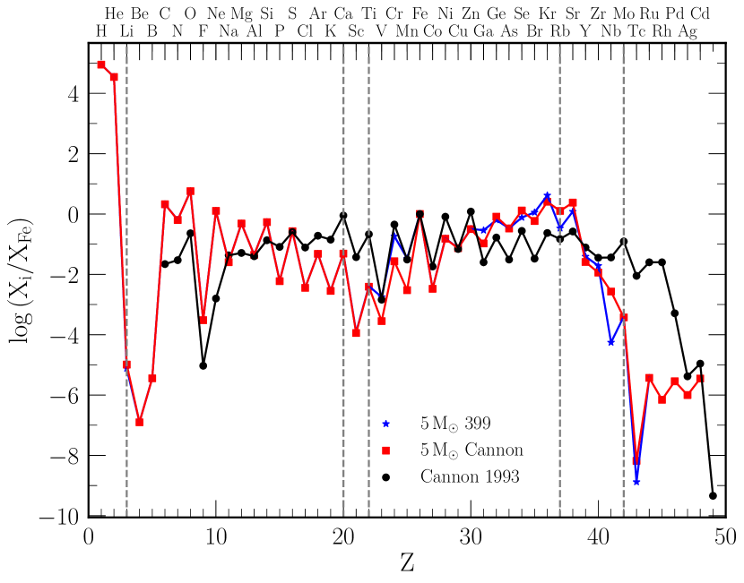
Figure 16: The surface composition relative to solar of a 5$\,\rm{M}_{\odot}$TŻO our default model assumptions (blue star) and a 5$\,\rm{M}_{\odot}$ model with a Cannon-like network (red square). This snapshot was taken at $\approx 10,000$ years post TŻO formation. In black dots, the Model A of C93. Vertical lines mark elements that may be useful for detecting TŻOs.

We have also run an additional network that is the one shown in figure 17 of C93, except we truncate at Cd, leaving 390 isotopes. Figure 16 shows the surface mass fractions of our 5$\,\rm{M}_{\odot}$ default model and a 5$\,\rm{M}_{\odot}$ model using the Cannon-like nuclear network. There is very little difference in the overall mass fractions except at V, Cr, Mn, and Nb.

By extending the network to Cd we see a sharp decline in the relative mass fraction of elements heavier than Pd in model A of C93. This is similar behaviour to what is seen in our models, albeit at a higher atomic number. Thus it appears that our models differ mostly by having the element with the highest production factor (Kr) at lower Z, compared to C93. This turn over to lower production factors then also occurs at lower atomic numbers.

Appendix C MESA physics options

Radiative opacities are primarily from OPAL (Iglesias & Rogers, 1993, 1996), with low-temperature data from Ferguson et al. (2005) and the high-temperature, Compton-scattering-dominated regime by Poutanen (2017). Electron conduction opacities are from Cassisi et al. (2007).

Nuclear reaction rates are a combination of rates from NACRE (Angulo et al., 1999), JINA REACLIB (Cyburt et al., 2010), plus additional tabulated weak reaction rates (Fuller et al., 1985; Oda et al., 1994; Langanke & Martínez-Pinedo, 2000). Screening is included via the prescription of Chugunov et al. (2007). Thermal neutrino loss rates are from Itoh et al. (1996).

Appendix D Surface mass fractions

Table 3 shows the surface chemical mass fractions from Figure 9(a). These are for a 5$\,\rm{M}_{\odot}$ TŻO, with a $1.4\,\,\rm{M}_{\odot}$ NS, and varying initial helium mass fraction. Values are quoted at 10,000 years after formation. The time evolution of the isotopic data is available in the Zenodo online material.

Table 3: Surface elemental mass fractions for the 399 isotope models with different $\rm{Y_{init}}$ values. mass fractions measured at 10,000 years post TŻO formation.

Element	$\rm{Y_{init}}=0.28$	$\rm{Y_{init}}=0.40$	$\rm{Y_{init}}=0.60$
H	7.194E-01	5.993E-01	3.991E-01
He	2.804E-01	4.005E-01	6.008E-01
Li	6.087E-11	6.105E-11	6.127E-11
Be	1.007E-12	1.010E-12	1.013E-12
B	2.886E-11	2.894E-11	2.903E-11
C	1.694E-05	1.701E-05	1.714E-05
N	5.115E-06	5.220E-06	5.422E-06
O	4.605E-05	4.617E-05	4.629E-05
F	2.443E-09	2.449E-09	2.456E-09
Ne	1.024E-05	1.026E-05	1.029E-05
Na	2.045E-07	2.050E-07	2.056E-07
Mg	3.883E-06	3.893E-06	3.904E-06
Al	3.552E-07	3.561E-07	3.571E-07
Si	4.328E-06	4.338E-06	4.350E-06
P	4.793E-08	4.805E-08	4.818E-08
S	2.160E-06	2.165E-06	2.171E-06
Cl	2.869E-08	2.875E-08	2.888E-08
Ar	3.850E-07	3.859E-07	3.871E-07
K	2.283E-08	2.288E-08	2.317E-08
Ca	3.934E-07	4.092E-07	4.990E-07
Sc	9.772E-10	2.419E-09	1.074E-08
Ti	3.252E-08	6.066E-08	2.027E-07
V	1.423E-08	3.899E-08	1.462E-07
Cr	1.467E-06	1.330E-06	7.577E-07
Mn	2.691E-07	4.975E-07	1.459E-06
Fe	8.010E-06	8.932E-06	1.181E-05
Co	2.666E-08	4.457E-08	1.266E-07
Ni	1.244E-06	3.187E-06	9.547E-06
Cu	5.966E-07	1.795E-06	3.881E-06
Zn	2.584E-06	7.746E-06	7.375E-06
Ga	2.307E-06	5.217E-06	1.428E-06
Ge	5.077E-06	1.017E-05	1.689E-06
As	2.688E-06	4.337E-06	3.025E-08
Se	6.139E-06	1.054E-05	1.111E-07
Br	9.040E-06	6.373E-06	3.187E-09
Kr	3.322E-05	7.479E-06	1.132E-09
Rb	2.707E-06	9.555E-09	9.490E-11
Sr	9.650E-06	2.832E-08	3.171E-10
Y	3.129E-07	7.296E-11	6.551E-11
Zr	1.542E-07	1.595E-10	1.589E-10
Nb	4.436E-10	1.014E-11	1.012E-11
Mo	3.195E-09	3.964E-11	3.963E-11
Tc	1.056E-14	1.274E-15	6.608E-17
Ru	2.988E-11	2.988E-11	2.988E-11

References

- Ablimit et al. (2022) Ablimit I., Podsiadlowski P., Hirai R., Wicker J., 2022, MNRAS, 513, 4802
- Ahmad et al. (2006) Ahmad I., Greene J. P., Moore E. F., Ghelberg S., Ofan A., Paul M., Kutschera W., 2006, Phys. Rev. C, 74, 065803
- Angulo et al. (1999) Angulo C., et al., 1999, Nuclear Physics A, 656, 3
- Asplund et al. (2009) Asplund M., Grevesse N., Sauval A. J., Scott P., 2009, ARA&A, 47, 481
- Audi et al. (2003) Audi G., Bersillon O., Blachot J., Wapstra A. H., 2003, Nuclear Phys. A, 729, 3
- Ayasli & Joss (1982) Ayasli S., Joss P. C., 1982, ApJ, 256, 637
- Baraffe et al. (2001) Baraffe I., Heger A., Woosley S. E., 2001, ApJ, 550, 890
- Beasor et al. (2018) Beasor E. R., Davies B., Cabrera-Ziri I., Hurst G., 2018, MNRAS, 479, 3101
- Biehle (1991) Biehle G. T., 1991, ApJ, 380, 167
- Biehle (1994) Biehle G. T., 1994, ApJ, 420, 364
- Bisnovatyi-Kogan & Lamzin (1984) Bisnovatyi-Kogan G. S., Lamzin S. A., 1984, Soviet Ast., 28, 187
- Breier et al. (2019) Breier A. A., Waßmuth B., Fuchs G. W., Gauss J., Giesen T. F., 2019, Journal of Molecular Spectroscopy, 355, 46
- Brünken et al. (2008) Brünken S., Müller H. S. P., Menten K. M., McCarthy M. C., Thaddeus P., 2008, ApJ, 676, 1367
- Cameron (1955) Cameron A. G. W., 1955, ApJ, 121, 144
- Cannon (1993) Cannon R. C., 1993, MNRAS, 263, 817
- Cannon et al. (1992) Cannon R. C., Eggleton P. P., Zytkow A. N., Podsiadlowski P., 1992, ApJ, 386, 206
- Cassisi et al. (2007) Cassisi S., Potekhin A. Y., Pietrinferni A., Catelan M., Salaris M., 2007, ApJ, 661, 1094
- Cholis et al. (2022) Cholis I., Kritos K., Garfinkle D., 2022, Phys. Rev. D, 105, 123022
- Chugunov et al. (2007) Chugunov A. I., Dewitt H. E., Yakovlev D. G., 2007, Phys. Rev. D, 76, 025028
- Clayton et al. (2017) Clayton M., Podsiadlowski P., Ivanova N., Justham S., 2017, MNRAS, 470, 1788
- Coe & Pightling (1998) Coe M. J., Pightling S. L., 1998, MNRAS, 299, 223
- Cox & Giuli (1968) Cox J. P., Giuli R. T., 1968, Principles of stellar structure
- Cyburt et al. (2010) Cyburt R. H., et al., 2010, ApJS, 189, 240
- Davies et al. (2018) Davies B., Crowther P. A., Beasor E. R., 2018, MNRAS, 478, 3138
- DeMarchi et al. (2021) DeMarchi L., Sanders J. R., Levesque E. M., 2021, ApJ, 911, 101
- Eich et al. (1989) Eich C., Zimmermann M. E., Thorne K. S., Zytkow A. N., 1989, ApJ, 346, 277
- Eisner et al. (2022) Eisner N. L., et al., 2022, MNRAS, 511, 4710
- Farag et al. (2020) Farag E., Timmes F. X., Taylor M., Patton K. M., Farmer R., 2020, ApJ, 893, 133
- Farmer et al. (2021) Farmer R., Laplace E., de Mink S. E., Justham S., 2021, ApJ, 923, 214
- Farmer et al. (2023) Farmer R., Laplace E., Ma J.-z., de Mink S. E., Justham S., 2023, ApJ, 948, 111
- Ferguson et al. (2005) Ferguson J. W., Alexander D. R., Allard F., Barman T., Bodnarik J. G., Hauschildt P. H., Heffner-Wong A., Tamanai A., 2005, ApJ, 623, 585
- Fisker et al. (2008) Fisker J. L., Schatz H., Thielemann F.-K., 2008, ApJS, 174, 261
- Fox & Wood (1982) Fox M. W., Wood P. R., 1982, ApJ, 259, 198
- Fryer et al. (1996) Fryer C. L., Benz W., Herant M., 1996, ApJ, 460, 801
- Fryer et al. (2014) Fryer C. L., Rueda J. A., Ruffini R., 2014, ApJ, 793, L36
- Fuller et al. (1985) Fuller G. M., Fowler W. A., Newman M. J., 1985, ApJ, 293, 1
- Goldberg et al. (2022) Goldberg J. A., Jiang Y.-F., Bildsten L., 2022, ApJ, 929, 156
- Grevesse & Sauval (1998) Grevesse N., Sauval A. J., 1998, Space Sci. Rev., 85, 161
- Grichener (2023) Grichener A., 2023, MNRAS, 523, 221
- Heger et al. (1997) Heger A., Jeannin L., Langer N., Baraffe I., 1997, A&A, 327, 224
- Herzberg (1950) Herzberg G., 1950, Molecular spectra and molecular structure. Vol.1: Spectra of diatomic molecules
- Hirai & Podsiadlowski (2022) Hirai R., Podsiadlowski P., 2022, MNRAS, 517, 4544
- Iglesias & Rogers (1993) Iglesias C. A., Rogers F. J., 1993, ApJ, 412, 752
- Iglesias & Rogers (1996) Iglesias C. A., Rogers F. J., 1996, ApJ, 464, 943
- Irwin (2004) Irwin A. W., 2004, The FreeEOS Code for Calculating the Equation of State for Stellar Interiors, http://freeeos.sourceforge.net/
- Itoh et al. (1996) Itoh N., Hayashi H., Nishikawa A., Kohyama Y., 1996, ApJS, 102, 411
- Iyudin et al. (1994) Iyudin A. F., et al., 1994, A&A, 284, L1
- Jermyn et al. (2021) Jermyn A. S., Schwab J., Bauer E., Timmes F. X., Potekhin A. Y., 2021, ApJ, 913, 72
- Jermyn et al. (2023) Jermyn A. S., et al., 2023, ApJS, 265, 15
- Kamiński et al. (2013) Kamiński T., et al., 2013, A&A, 551, A113
- Keek et al. (2009) Keek L., Langer N., in’t Zand J. J. M., 2009, A&A, 502, 871
- Kiss et al. (2006) Kiss L. L., Szabó G. M., Bedding T. R., 2006, MNRAS, 372, 1721
- Kremer et al. (2020) Kremer K., et al., 2020, ApJS, 247, 48
- Kuchner et al. (2002) Kuchner M. J., Vakil D., Smith V. V., Lambert D. L., Plez B., Phinney E. S., 2002, in Shara M. M., ed., Astronomical Society of the Pacific Conference Series Vol. 263, Stellar Collisions, Mergers and their Consequences. p. 131
- Langanke & Martínez-Pinedo (2000) Langanke K., Martínez-Pinedo G., 2000, Nuclear Physics A, 673, 481
- Leonard et al. (1994) Leonard P. J. T., Hills J. G., Dewey R. J., 1994, ApJ, 423, L19
- Levesque et al. (2005) Levesque E. M., Massey P., Olsen K. A. G., Plez B., Josselin E., Maeder A., Meynet G., 2005, ApJ, 628, 973
- Levesque et al. (2014) Levesque E. M., Massey P., Zytkow A. N., Morrell N., 2014, MNRAS, 443, L94
- Lincowski et al. (2016) Lincowski A. P., Halfen D. T., Ziurys L. M., 2016, ApJ, 833, 9
- Liu et al. (2015) Liu X. W., Xu R. X., van den Heuvel E. P. J., Qiao G. J., Han J. L., Han Z. W., Li X. D., 2015, ApJ, 799, 233
- Maccarone & de Mink (2016) Maccarone T. J., de Mink S. E., 2016, MNRAS, 458, L1
- Magkotsios et al. (2010) Magkotsios G., Timmes F. X., Hungerford A. L., Fryer C. L., Young P. A., Wiescher M., 2010, ApJS, 191, 66
- McKemmish et al. (2019) McKemmish L. K., Masseron T., Hoeijmakers H. J., Pérez-Mesa V., Grimm S. L., Yurchenko S. N., Tennyson J., 2019, MNRAS, 488, 2836
- Metzger (2022) Metzger B. D., 2022, ApJ, 932, 84
- Miller et al. (2019) Miller M. C., et al., 2019, ApJ, 887, L24
- Morán-Fraile et al. (2023) Morán-Fraile J., Schneider F. R. N., Röpke F. K., Ohlmann S. T., Pakmor R., Soultanis T., Bauswein A., 2023, A&A, 672, A9
- Moriya (2018) Moriya T. J., 2018, MNRAS, 475, L49
- Moriya & Blinnikov (2021) Moriya T. J., Blinnikov S. I., 2021, MNRAS, 508, 74
- Nakauchi et al. (2020) Nakauchi D., Inayoshi K., Omukai K., 2020, ApJ, 902, 81
- Nazin & Postnov (1995) Nazin S. N., Postnov K. A., 1995, A&A, 303, 789
- O’Grady et al. (2020) O’Grady A. J. G., et al., 2020, ApJ, 901, 135
- O’Grady et al. (2023) O’Grady A. J. G., et al., 2023, ApJ, 943, 18
- Oda et al. (1994) Oda T., Hino M., Muto K., Takahara M., Sato K., 1994, Atomic Data and Nuclear Data Tables, 56, 231
- Oppenheimer & Volkoff (1939) Oppenheimer J. R., Volkoff G. M., 1939, Physical Review, 55, 374
- Paczyński (1969) Paczyński B., 1969, Acta Astron., 19, 1
- Papish et al. (2015) Papish O., Soker N., Bukay I., 2015, MNRAS, 449, 288
- Patton et al. (2017a) Patton K. M., Lunardini C., Farmer R. J., 2017a, ApJ, 840, 2
- Patton et al. (2017b) Patton K. M., Lunardini C., Farmer R. J., Timmes F. X., 2017b, ApJ, 851, 6
- Pavlenko et al. (2020) Pavlenko Y. V., Yurchenko S. N., McKemmish L. K., Tennyson J., 2020, A&A, 642, A77
- Paxton et al. (2011) Paxton B., Bildsten L., Dotter A., Herwig F., Lesaffre P., Timmes F., 2011, ApJS, 192, 3
- Paxton et al. (2013) Paxton B., et al., 2013, ApJS, 208, 4
- Paxton et al. (2015) Paxton B., et al., 2015, ApJS, 220, 15
- Paxton et al. (2018) Paxton B., et al., 2018, ApJS, 234, 34
- Paxton et al. (2019) Paxton B., et al., 2019, ApJS, 243, 10
- Petersen (1973) Petersen J. O., 1973, A&A, 27, 89
- Piro & Bildsten (2007) Piro A. L., Bildsten L., 2007, ApJ, 663, 1252
- Podsiadlowski et al. (1995) Podsiadlowski P., Cannon R. C., Rees M. J., 1995, MNRAS, 274, 485
- Poutanen (2017) Poutanen J., 2017, ApJ, 835, 119
- Qin et al. (1998) Qin B., Wu X.-P., Chu M.-C., Fang L.-Z., Hu J.-Y., 1998, ApJ, 494, L57
- Ray et al. (1987) Ray A., Kembhavi A. K., Antia H. M., 1987, A&A, 184, 164
- Renzo & Götberg (2021) Renzo M., Götberg Y., 2021, ApJ, 923, 277
- Renzo et al. (2017) Renzo M., Ott C. D., Shore S. N., de Mink S. E., 2017, A&A, 603, A118
- Renzo et al. (2019) Renzo M., et al., 2019, A&A, 624, A66
- Renzo et al. (2023) Renzo M., Zapartas E., Justham S., Breivik K., Lau M., Farmer R., Cantiello M., Metzger B. D., 2023, ApJ, 942, L32
- Schneider et al. (2019) Schneider F. R. N., Ohlmann S. T., Podsiadlowski P., Röpke F. K., Balbus S. A., Pakmor R., Springel V., 2019, Nature, 574, 211
- Schrøder et al. (2020) Schrøder S. L., MacLeod M., Loeb A., Vigna-Gómez A., Mandel I., 2020, ApJ, 892, 13
- Serindag et al. (2021) Serindag D. B., Snellen I. A. G., Mollière P., 2021, A&A, 655, A69
- Soraisam et al. (2018) Soraisam M. D., et al., 2018, ApJ, 859, 73
- Soszyński et al. (2004) Soszyński I., Udalski A., Kubiak M., Szymański M., Pietrzyński G., Żebruń K., Szewczyk O., Wyrzykowski Ł., 2004, Acta Astron., 54, 129
- Soszyński et al. (2009) Soszyński I., et al., 2009, Acta Astron., 59, 239
- Soszyński et al. (2011) Soszyński I., et al., 2011, Acta Astron., 61, 217
- Steiner et al. (2010) Steiner A. W., Lattimer J. M., Brown E. F., 2010, ApJ, 722, 33
- Taam et al. (1978) Taam R. E., Bodenheimer P., Ostriker J. P., 1978, ApJ, 222, 269
- Tabernero et al. (2021) Tabernero H. M., Dorda R., Negueruela I., Marfil E., 2021, A&A, 646, A98
- Terman et al. (1995) Terman J. L., Taam R. E., Hernquist L., 1995, ApJ, 445, 367
- Thorne (1977) Thorne K. S., 1977, ApJ, 212, 825
- Thorne & Zytkow (1975) Thorne K. S., Zytkow A. N., 1975, ApJ, 199, L19
- Thorne & Zytkow (1977) Thorne K. S., Zytkow A. N., 1977, ApJ, 212, 832
- Timmes & Swesty (2000) Timmes F. X., Swesty F. D., 2000, ApJS, 126, 501
- Timmes et al. (1996) Timmes F. X., Woosley S. E., Hartmann D. H., Hoffman R. D., 1996, ApJ, 464, 332
- Tout et al. (2014) Tout C. A., Zytkow A. N., Church R. P., Lau H. H. B., Doherty C. L., Izzard R. G., 2014, MNRAS, 445, L36
- Townsend & Teitler (2013) Townsend R. H. D., Teitler S. A., 2013, MNRAS, 435, 3406
- Townsend et al. (2018) Townsend R. H. D., Goldstein J., Zweibel E. G., 2018, MNRAS, 475, 879
- Tuchman et al. (1978) Tuchman Y., Sack N., Barkat Z., 1978, ApJ, 219, 183
- Tuchman et al. (1979) Tuchman Y., Sack N., Barkat Z., 1979, ApJ, 234, 217
- Vanture et al. (1999) Vanture A. D., Zucker D., Wallerstein G., 1999, ApJ, 514, 932
- Wallace & Woosley (1981) Wallace R. K., Woosley S. E., 1981, ApJS, 45, 389
- Witsch et al. (2021) Witsch D., Breier A. A., Döring E., Yamada K. M. T., Giesen T. F., Fuchs G. W., 2021, Journal of Molecular Spectroscopy, 377, 111439
- Xin et al. (2022) Xin C., Renzo M., Metzger B. D., 2022, MNRAS, 516, 5816
- Yoon & Cantiello (2010) Yoon S.-C., Cantiello M., 2010, ApJ, 717, L62
- van Loon et al. (2005) van Loon J. T., Cioni M. R. L., Zijlstra A. A., Loup C., 2005, A&A, 438, 273
- van Paradijs et al. (1995) van Paradijs J., Spruit H. C., van Langevelde H. J., Waters L. B. F. M., 1995, A&A, 303, L25
- van Wormer et al. (1994) van Wormer L., Görres J., Iliadis C., Wiescher M., Thielemann F. K., 1994, ApJ, 432, 326