Weighted scoringRules: Emphasising Particular Outcomes when Evaluating Probabilistic Forecasts

Sam Allen Weighted scoringRules: Emphasising Particular Outcomes when Evaluating Probabilistic Forecasts Weighted scoringRules When predicting future events, it is common to issue forecasts that are probabilistic, in the form of probability distributions over the range of possible outcomes. Such forecasts can be evaluated using proper scoring rules. Proper scoring rules condense forecast performance into a single numerical value, allowing competing forecasters to be ranked and compared. To facilitate the use of scoring rules in practical applications, the scoringRules package in R provides popular scoring rules for a wide range of forecast distributions. This paper discusses an extension to the scoringRules package that additionally permits the implementation of popular weighted scoring rules. Weighted scoring rules allow particular outcomes to be targeted during forecast evaluation, recognising that certain outcomes are often of more interest than others when assessing forecast quality. This introduces the potential for very flexible, user-oriented evaluation of probabilistic forecasts. We discuss the theory underlying weighted scoring rules, and describe how they can readily be implemented in practice using scoringRules. Functionality is available for weighted versions of several popular scoring rules, including the logarithmic score, the continuous ranked probability score (CRPS), and the energy score. Two case studies are presented to demonstrate this, whereby weighted scoring rules are applied to univariate and multivariate probabilistic forecasts in the fields of meteorology and economics. forecast evaluation, probabilistic forecasting, proper scoring rules, weighted scoring rules, R forecast evaluation, probabilistic forecasting, proper scoring rules, weighted scoring rules, R Sam Allen
University of Bern
Institute of Mathematical Statistics and Actuarial Science
Alpeneggstrasse 22
3012 Bern, Switzerland
E-Mail:
and
Oeschger Centre for Climate Change Research

1 Introduction: Weighted scoring rules

When predicting future events, it is common to issue forecasts that are probabilistic. Probabilistic forecasts generally take the form of probability distributions over the range of possible outcomes, comprehensively describing the predictive uncertainty. To assess the quality of a probabilistic forecast, scoring rules are functions $S(F,y)$ that take a forecast $F$ and the corresponding outcome $y$ as inputs, and output a numerical score that quantifies the forecast’s accuracy. Scoring rules therefore condense forecast performance into a single value, providing a convenient framework with which to objectively rank and compare competing forecasts. As such, scoring rules have become a key component of probabilistic forecast evaluation.

To assess probabilistic forecasts in practice, the scoringRules package (JordanEtAl2018) in the programming language R has become a widely used resource. The package contains analytical formulae for the two most popular univariate scoring rules — the logarithmic score (LogS; Good1952) and the continuous ranked probability score (CRPS; MathesonWinkler1976) — for forecast distributions belonging to a range of parametric families. These scoring rules are also available when the forecast is a sample from a predictive distribution, which is often the case in practice. The scoringRules package additionally allows samples from multivariate forecast distributions to be evaluated using popular multivariate scoring rules, including the energy score (GneitingRaftery2007), variogram score (ScheuererHamill2015), and a kernel score based on the Gaussian kernel (GneitingRaftery2007).

The scoring rules listed above assess forecasts made for all outcomes. While this is clearly desirable when assessing overall forecast performance, it is often the case that certain outcomes are of more interest than others. For example, one could argue that it is particularly important to issue accurate forecasts for outcomes that have a high impact on the forecast users. To emphasise particular outcomes during forecast evaluation, weighted scoring rules generalise conventional scoring rules by incorporating a weight function into the score. The weight function can be chosen such that a higher weight is assigned to outcomes that are of more interest. Weighted scoring rules therefore allow competing forecast systems to be ranked and compared when predicting particular outcomes, facilitating very flexible, user-oriented forecast evaluation.

Well known examples of weighted scoring rules include the conditional and censored likelihood scores proposed by DiksEtAl2011, and the threshold-weighted CRPS introduced by MathesonWinkler1976 and GneitingRanjan2011. However, the theory underlying weighted scoring rules extends beyond these examples: HolzmannKlar2017 demonstrate that the conditional and censored likelihood scores can be generalised to construct weighted versions of any proper scoring rule, while AllenEtAl2022 introduce a broad generalisation of the threshold-weighted CRPS that can be applied, for example, to probabilistic forecasts for multivariate outcomes.

In this paper, we describe how the scoringRules package has been extended to additionally permit the implementation of popular weighted scoring rules. While several alternative software packages exist to calculate particular scoring rules in certain situations (see JordanEtAl2018, for an overview), the development of weighted scoring rules is more recent. Until recently, for example, efficient application of popular weighted scoring rules was limited by theoretical considerations, leading to ad hoc implementations in practice (SharpeEtAl2018). Hence, to our knowledge, no other packages exist that provide a comprehensive collection of weighted scoring rules. We therefore hope that this extension to scoringRules will greatly facilitate the successful implementation of weighted scoring rules in practical applications.

In the following section, we review the existing theory of weighted scoring rules, and introduce examples of weighted versions of several popular scores, such as the LogS, the CRPS, and the energy score. The remainder of the paper then illustrates how these weighted scoring rules can be implemented in practice using the scoringRules package. Section 3 outlines the functionality of the package when calculating weighted scoring rules, and discusses implementation options. Section LABEL:sec:examples then presents two case studies in which these weighted scoring rules are used to target particular outcomes when evaluating probabilistic forecasts in practice. These case studies include applications in weather forecasting and economic forecasting, building on the examples presented in JordanEtAl2018. A summary of the paper is presented in Section LABEL:sec:summary.

2 Theoretical background

2.1 Proper scoring rules

Suppose we are interested in predicting a random variable $Y$ that takes values in a set $\Omega$, and that our forecasts are in the form of probability distributions over $\Omega$. Let $\mathcal{F}$ denote a set of such forecasts. A scoring rule is a function

$$S:\mathcal{F}\times\Omega\to\mathbb{R}\cup\{-\infty,\infty\},$$

which takes a forecast $F\in\mathcal{F}$ and an observation $y\in\Omega$ as inputs, and outputs a numerical value, or score, that quantifies the forecast accuracy. A lower score is assigned to a more accurate forecast. A scoring rule is proper with respect to $\mathcal{F}$ if, when the observations are drawn from a distribution $G\in\mathcal{F}$, the scoring rule is minimised in expectation by issuing $G$ as the forecast, i.e.

$$\E_{Y\sim G}S(G,Y)\leq\E_{Y\sim G}S(F,Y)$$

for all $F,G\in\mathcal{F}$. If the above inequality is strict, then $S$ is strictly proper with respect to $\mathcal{F}$.

When the outcome variable is real-valued ($\Omega\subseteq\mathbb{R}$), probabilistic forecasts are typically evaluated using either the logarithmic score (LogS) or the continuous ranked probability score (CRPS). The LogS is defined as

$$\mathrm{LogS}(F,y)=-\mathrm{log}f(y),$$ (1)

where $f$ is the predictive density associated with the cumulative distribution function $F$ (Good1952). The CRPS is defined as

$$\begin{split}\operatorname{CRPS}(F,y)&=\int_{\mathbb{R}}(F(z)-\mathbbm{1}\{y\leq z\})^{2}\hskip 2.84544pt\mathrm{d}z\\ &=\E_{F}|X-y|-\frac{1}{2}\E_{F}|X-X^{\prime}|,\end{split}$$ (2)

where $\mathbbm{1}$ is the indicator function, $X,X^{\prime}\sim F$ are independent random variables, and it is assumed in the second expression that $F$ has a finite mean (MathesonWinkler1976; GneitingRaftery2007).

Generalisations of the LogS and the CRPS are also commonly used to evaluate probabilistic forecasts for multivariate outcomes, i.e. $\Omega\subseteq\mathbb{R}^{d}$ for $d>1$. While the LogS in Equation 1 can readily be applied to multivariate predictive densities, it is often the case that only a sample from the multivariate forecast distribution is available, making it difficult to employ the LogS in practice. Instead, alternative scoring rules have been proposed to evaluate multivariate probabilistic forecasts that can readily be applied to samples from a forecast distribution.

Arguably the most well known multivariate scoring rule is the energy score (ES; GneitingRaftery2007), which generalises the CRPS to higher dimensions:

$$\mathrm{ES}(F,\mathbf{y})=\E_{F}\|\mathbf{X}-\mathbf{y}\|-\frac{1}{2}\E_{F}\|\mathbf{X}-\mathbf{X}^{\prime}\|,$$ (3)

where $\|\cdot\|$ is the Euclidean distance in $\mathbb{R}^{d}$, $\mathbf{y}=(y_{1},\dots,y_{d})\in\Omega$, and $\mathbf{X}=\left(X_{1},\dots,X_{d}\right)$, $\mathbf{X}^{\prime}=\left(X_{1}^{\prime},\dots,X_{d}^{\prime}\right)\sim F$ are independent, with $F$ a probability distribution on $\Omega$. It is assumed here and throughout that the expectations are finite where necessary.

An alternative to the energy score is the variogram score (VS; ScheuererHamill2015). The variogram score aims to explicitly assess the dependence structure of the multivariate forecast distributions by measuring the distance between the variogram of the forecast and that of the observation. The variogram score of order $p>0$ is defined as

$$\mathrm{VS}^{p}(F,\mathbf{y})=\sum_{i=1}^{d}\sum_{j=1}^{d}h_{i,j}\left(\E_{F}\left|X_{i}-X_{j}\right|^{p}-\left|y_{i}-y_{j}\right|^{p}\right)^{2},$$ (4)

where $\mathbf{X}=\left(X_{1},\dots,X_{d}\right)\sim F$, $\mathbf{y}=\left(y_{1},\dots,y_{d}\right)\in\Omega$, and $h_{i,j}$ are non-negative scaling parameters that control how much emphasis is given to a pair of dimensions. Following recommendations from ScheuererHamill2015, the order of the score, $p$, is often chosen to be 0.5.

Both the energy score and the variogram score belong to the very general class of kernel scores (GneitingRaftery2007). Kernel scores are scoring rules that are constructed using conditionally negative definite kernels, and the kernel score framework has also been leveraged to introduce alternative multivariate scoring rules. AllenEtAl2022, for example, introduced a multivariate scoring rule based on the inverse multiquadric kernel, while the so-called maximum mean discrepancy score (MMDS) is the kernel score corresponding to the Gaussian kernel:

$$\mathrm{MMDS}(F,\mathbf{y})=\frac{1}{2}\E_{F}\left[\mathrm{exp}\left\{-\frac{1}{2}\|\mathbf{X}-\mathbf{X}^{\prime}\|^{2}\right\}\right]-\E_{F}\left[\mathrm{exp}\left\{-\frac{1}{2}\|\mathbf{X}-\mathbf{y}\|^{2}\right\}\right],$$ (5)

where $\mathbf{X},\mathbf{X}^{\prime}\sim F$ are independent.

To facilitate the implementation of these popular scoring rules in practice, the scoringRules package provides analytical expressions of the LogS and CRPS for forecasts that correspond to several familiar parametric distributions. It is also often the case that only a sample from the forecast distribution is available; this is common, for example, when considering ensemble forecasts issued by numerical weather and climate models, or output from Markov chain Monte Carlo (MCMC) algorithms (KruegerEtAl2021). The scoringRules package therefore additionally contains versions of the LogS, CRPS, ES, VS, and MMDS that can be used to evaluate forecasts in the form of a predictive sample. This can be achieved by replacing the expectations in Equations 2-5 with sample means (see Appendix LABEL:app:sampleformulas for details). For the LogS, kernel density estimation is used to estimate the predictive density from the sample, prior to calculating the score.

2.2 Weighted scoring rules

The scoring rules introduced in the previous section evaluate the entire forecast distribution. However, one could argue that it is particularly important to issue accurate forecasts for events that have a high impact on the forecast users, and such events should therefore be given more weight during forecast evaluation. Weighted scoring rules achieve this by incorporating a non-negative weight function $w$ into conventional scoring rules, where the weight function determines how much emphasis should be placed on each possible outcome. Different approaches to weight scoring rules exist, and here we focus only on the two most popular frameworks.

2.2.1 Outcome-weighted scoring rules

DiksEtAl2011 introduced two weighted versions of the LogS that allow particular outcomes to be emphasised when calculating forecast accuracy. The conditional likelihood score (CoLS) is defined as

$$\mathrm{CoLS}(F,y)=-w(y)\mathrm{log}f(y)+w(y)\mathrm{log}\left(\int_{\mathbb{R}}w(z)f(z)\hskip 2.84544pt\mathrm{d}z\right),$$

while the censored likelihood score (CeLS) is

$$\mathrm{CeLS}(F,y)=-w(y)\mathrm{log}f(y)-(1-w(y))\mathrm{log}\left(1-\int_{\mathbb{R}}w(z)f(z)\hskip 2.84544pt\mathrm{d}z\right).$$

To understand how these weighted logarithmic scores behave, consider a weight function of the form $w(z)=\mathbbm{1}\{z\in\mathcal{A}\}$, meaning only forecasts for outcomes in the set $\mathcal{A}\subseteq\mathbb{R}$ are of interest. In this example, if the observation $y\notin\mathcal{A}$, then the CoLS is equal to zero, so that only the forecasts issued when $y\in\mathcal{A}$ contribute to the score. If $y\in\mathcal{A}$, then the CoLS is equivalent to the LogS applied to the conditional forecast distribution given that the observation is in $\mathcal{A}$; forecast distributions are therefore assessed only via their restriction to the set $\mathcal{A}$. The CeLS then extends the CoLS by additionally rewarding forecast distributions that can correctly predict when an outcome of interest will or will not occur. Note that if $\mathcal{A}=\mathbb{R}$, then the weight function is always one, and both weighted scoring rules revert to the unweighted LogS.

HolzmannKlar2017 later generalised the CoLS and CeLS by demonstrating that this framework can readily be applied to any proper scoring rule. The resulting scoring rules, which we call outcome-weighted scoring rules, target particular outcomes by introducing a weighted version of the forecast distribution, and evaluating $F$ via its weighted representation. For the weight function $w(z)=\mathbbm{1}\{z\in\mathcal{A}\}$, this weighted representation is simply the conditional distribution given that the outcome is in $\mathcal{A}$, as discussed above for the CoLS and CeLS. Further details can be found in HolzmannKlar2017.

An outcome-weighted CRPS can be defined as

$$\mathrm{owCRPS}(F,y)=\frac{1}{\bar{w}_{F}}\E_{F}\left[|X-y|w(X)w(y)\right]-\frac{1}{2\bar{w}_{F}^{2}}\E_{F}\left[|X-X^{\prime}|w(X)w(X^{\prime})w(y)\right],$$

where $X,X^{\prime}\sim F$ are independent and $\bar{w}_{F}=\E_{F}[w(X)]$. Since this framework applies to any proper scoring rule, outcome-weighted versions of the ES, VS, and MMDS can similarly be introduced to target multivariate outcomes of interest during forecast evaluation:

$$\begin{split}\mathrm{owES}(F,\mathbf{y})=&\frac{1}{\bar{w}_{F}}\E_{F}\left[\|\mathbf{X}-\mathbf{y}\|w(\mathbf{X})w(\mathbf{y})\right]-\frac{1}{2\bar{w}_{F}^{2}}\E_{F}\left[\|\mathbf{X}-\mathbf{X}^{\prime}\|w(\mathbf{X})w(\mathbf{X}^{\prime})w(\mathbf{y})\right];\\ \mathrm{owVS}^{p}(F,\mathbf{y})=&w(\mathbf{y})\sum_{i=1}^{d}\sum_{j=1}^{d}h_{i,j}\left(\frac{1}{\bar{w}_{F}}\E_{F}\left[\left|X_{i}-X_{j}\right|^{p}w(\mathbf{X})\right]-\left|y_{i}-y_{j}\right|^{p}\right)^{2};\\ \mathrm{owMMDS}(F,\mathbf{y})=&\frac{1}{2\bar{w}_{F}^{2}}\E_{F}\left[\mathrm{exp}\left\{-\frac{1}{2}\|\mathbf{X}-\mathbf{X}^{\prime}\|^{2}\right\}w(\mathbf{X})w(\mathbf{X}^{\prime})w(\mathbf{y})\right]\\ &-\frac{1}{\bar{w}_{F}}\E_{F}\left[\mathrm{exp}\left\{-\frac{1}{2}\|\mathbf{X}-\mathbf{y}\|^{2}\right\}w(\mathbf{X})w(\mathbf{y})\right].\end{split}$$

Note that in the multivariate case, the weight function takes a vector as an argument; $\bar{w}_{F}$ is thus defined as $\bar{w}_{F}=\E_{F}[w(\mathbf{X})]$.

The premise behind this class of weighted scoring rules is that, if attention is only on a particular set of outcomes, then the forecasts are only evaluated when these outcomes occur. When these outcomes do occur, the forecast distributions are evaluated using the conditional distribution given that the outcome of interest has occurred. In considering the conditional distribution given that an outcome of interest has occurred, the score does not consider the predicted probability that this outcome will occur. The CeLS extends the CoLS to address this, and suitable adaptations of the larger class of outcome-weighted scoring rules also exist, though these are not considered here (see HolzmannKlar2017).

Moreover, these scores are clearly not well-defined if the conditional distribution does not exist. This is equivalent to $\bar{w}_{F}$ being equal to zero, which could occur, for example, if $w(z)=\mathbbm{1}\{z\in\mathcal{A}\}$ and the forecast distribution assigns zero probability to the region $\mathcal{A}$. The use of these outcome-weighted scoring rules is therefore only recommended when the weight function is strictly positive, or when interest is on events that are not rare, such that $\bar{w}_{F}$ is non-zero (AllenEtAl2023).

2.2.2 Threshold-weighted scoring rules

Arguably the most well known weighted scoring rule is the threshold-weighted CRPS proposed by MathesonWinkler1976 and GneitingRanjan2011. The threshold-weighted CRPS introduces a weight function into the integral defining the CRPS:

$$\begin{split}\mathrm{twCRPS}(F,y)&=\int_{\mathbb{R}}(F(z)-\mathbbm{1}\{y\leq z\})^{2}w(z)\hskip 2.84544pt\mathrm{d}z\\ &=\E_{F}|v(X)-v(y)|-\frac{1}{2}\E_{F}|v(X)-v(X^{\prime})|,\end{split}$$

where $v$ is any function such that $v(z)-v(z^{\prime})=\int_{z^{\prime}}^{z}w(z)\hskip 2.84544pt\mathrm{d}z$ for all $z,z^{\prime}\in\mathbb{R}$ (TaillardatEtAl2022; AllenEtAl2022). We follow AllenEtAl2022 and refer to $v$ as a chaining function.

Just as we can generate outcome-weighted versions of any proper scoring rule, AllenEtAl2022 demonstrate that the theory underlying the threshold-weighted CRPS can readily be extended to any kernel score. As discussed, the ES, VS, and MMDS are all kernel scores, allowing threshold-weighted versions of these scores to be introduced:

$$\begin{split}\mathrm{twES}(F,\mathbf{y})=&\E_{F}\|v(\mathbf{X})-v(\mathbf{y})\|-\frac{1}{2}\E_{F}\|v(\mathbf{X})-v(\mathbf{X}^{\prime})\|;\\ \mathrm{twVS}^{p}(F,\mathbf{y})=&\sum_{i=1}^{d}\sum_{j=1}^{d}h_{i,j}\left(\E_{F}\left|v(\mathbf{X})_{i}-v(\mathbf{X})_{j}\right|^{p}-\left|v(\mathbf{y})_{i}-v(\mathbf{y})_{j}\right|^{p}\right)^{2};\\ \mathrm{twMMDS}(F,\mathbf{y})=&\frac{1}{2}\E_{F}\left[\mathrm{exp}\left\{-\frac{1}{2}\|v(\mathbf{X})-v(\mathbf{X}^{\prime})\|^{2}\right\}\right]-\E_{F}\left[\mathrm{exp}\left\{-\frac{1}{2}\|v(\mathbf{X})-v(\mathbf{y})\|^{2}\right\}\right],\end{split}$$ (6)

where $\mathbf{X},\mathbf{X}^{\prime}\sim F$ are independent random variables taking values on $\Omega\subseteq\mathbb{R}^{d}$, and $v:\mathbb{R}^{d}\to\mathbb{R}^{d}$ is a chaining function, so that $v(\mathbf{y})=\left(v(\mathbf{y})_{1},\dots,v(\mathbf{y})_{d}\right)$ and likewise for $v(\mathbf{X})$ and $v(\mathbf{X}^{\prime})$.

In contrast to the outcome-weighted scoring rules, threshold-weighted scoring rules transform the forecasts and observations according to a chaining function $v$ prior to employing the unweighted version of the scores. The chaining function can therefore be chosen to focus the scoring rules on particular outcomes. While there exists a canonical way to obtain a chaining function from a given weight function in the univariate case, no such relationship exists when evaluating multivariate forecasts. This is discussed further in the following section.

2.3 Weight and chaining functions

These weighted scoring rules provide attractive ways to target particular outcomes of interest when evaluating forecast performance, both in the univariate and multivariate case. In this section, we discuss possible weight and chaining functions that can be used within these weighted scoring rules. Certain choices can result in weighted scoring rules that are not proper, and these weight and chaining functions must therefore be chosen with care, to ensure that forecasters are not evaluated using an improper scoring rule.

If both a weighted and unweighted version of a scoring rule are proper, then they will both be minimised on average by the same forecast distribution: the true distribution of the outcome. However, for two imperfect forecasts, the ranking of these forecasts may change depending on whether a weighted or unweighted scoring rule is employed. Weighted scoring rules may be less powerful than conventional scoring rules when discriminating between two forecast distributions, but they should be more discriminative when comparing forecasts made for particular outcomes. Put differently, if weighted scoring rules detect a difference between two forecast systems, then it is generally easier to interpret this difference than if it were detected using an unweighted scoring rule.

Readers are referred to GneitingRanjan2011, LerchEtAl2017, and AllenEtAl2022 for further details regarding what weight and chaining functions preserve the (strict) propriety of scoring rules. The weight and chaining functions that we consider here all result in weighted scoring rules that are themselves proper (though not necessarily strictly proper).

2.3.1 Weight functions

The choice of weight and chaining function is case-specific, and should depend on what information is to be extracted from the forecasts. Most commonly, interest is on outcomes within a certain range, or above or below a predefined threshold; this range or threshold may correspond to relevant quantiles of the previously observed outcomes. A univariate weight function that restricts attention to these events is

$$w(z)=\mathbbm{1}\{a<z<b\}\quad\text{for some}\quad-\infty\leq a<b\leq\infty,$$ (7)

which is one if $z$ is between $a$ and $b$, and zero otherwise. To emphasise values above (below) some threshold $t$, we can set $a=t$ and $b=\infty$ ($a=-\infty$ and $b=t$).

Alternatively, certain events could be emphasised using a smoother weight function, which assigns a positive weight to all outcomes, but a higher weight to the events of interest. Popular weight functions to emphasise rare events include a Gaussian or logistic distribution function, e.g.

$$w(z)=\Phi_{\mu,\sigma}(z),$$ (8)

where $\Phi_{\mu,\sigma}$ is the Gaussian distribution function with mean $\mu$ and standard deviation $\sigma$, with these parameters controlling the location of the weight function and the rate at which it tends to zero and one (GneitingRanjan2011).

Gaussian and logistic density functions could additionally be used to target outcomes that are not rare. For example, the weight function

$$w(z)=\phi_{\mu,\sigma}(z),$$

where $\phi_{\mu,\sigma}$ is the Gaussian density function with mean $\mu$ and standard deviation $\sigma$. This weight function will emphasise values around the location parameter $\mu$, with $\sigma$ determining the concentration of the weight around $\mu$.

Similar weight functions can also be used in the multivariate case. For example, it is common to define rare multivariate events as threshold exceedances that occur simultaneously in multiple dimensions, in which case a canonical weight function is

$$w(\mathbf{z})=\mathbbm{1}\{a_{1}<z_{1}<b_{1},\dots,a_{d}<z_{d}<b_{d}\}\quad\text{for}\quad-\infty\leq a_{i}<b_{i}\leq\infty,\quad i=1,\dots,d.$$ (9)

As in the univariate case, some values of the vectors $\mathbf{a}=(a_{1},\dots,a_{d})$ and $\mathbf{b}=(b_{1},\dots,b_{d})$ can be set to $\pm\infty$ in order to focus on threshold exceedances. Multivariate Gaussian distribution and density functions could then again be used to target particular regions of multivariate space in a smoother way (AllenEtAl2023). These weight functions are listed in Table 1.

Weight function	Chaining function
$w(z)=1$	$v(z)=z$
$w(z)=\mathbbm{1}\{a<z<b\}$	$v(z)=\min(\max(z,a),b)$
$w(z)=\Phi_{\mu,\sigma}(z)$	$v(z)=(z-\mu)\Phi_{\mu,\sigma}(z)+\sigma^{2}\phi_{\mu,\sigma}(z)$
$w(z)=\phi_{\mu,\sigma}(z)$	$v(z)=\Phi_{\mu,\sigma}(z)$
$w(\boldsymbol{z})=\mathbbm{1}\left\{a_{1}<z_{1}<b_{1},\dots,a_{d}<z_{d}<b_{d}\right\}$	$v(\boldsymbol{z})_{i}=\min(\max(z_{i},a_{i}),b_{i})$
$w(\boldsymbol{z})=\boldsymbol{\Phi_{\mu,\Sigma}}(\boldsymbol{z})$	$v(\boldsymbol{z})_{i}=(z_{i}-\mu_{i})\Phi_{\mu_{i},\sigma_{i}}(z_{i})+\sigma_{i}^{2}\phi_{\mu_{i},\sigma_{i}}(z_{i})$
$w(\boldsymbol{z})=\boldsymbol{\phi_{\mu,\Sigma}}(\boldsymbol{z})$	$v(\boldsymbol{z})_{i}=\Phi_{\mu_{i},\sigma_{i}}(z_{i})$

Table 1: Examples of weight functions and chaining functions that could be used in weighted scoring rules. $\boldsymbol{\Phi_{\mu,\Sigma}}$ and $\boldsymbol{\phi_{\mu,\Sigma}}$ denote the multivariate Gaussian distribution and density functions with mean vector $\boldsymbol{\mu}=(\mu_{1},\dots,\mu_{d})$ and covariance matrix $\Sigma$ with diagonal entries $\sigma_{1},\dots,\sigma_{d}$. The multivariate chaining functions are component-wise extensions of the univariate chaining functions; hence, for concision, only the $i$-th component (for $i\in\{1,\dots,d\}$) of the multivariate chaining function is shown.

2.3.2 Chaining functions

While the outcome-weighted scoring rules depend on a weight function, the threshold-weighted scoring rules depend on a chaining function. It is arguably less intuitive to choose a chaining function to emphasise certain outcomes of interest than a weight function. In the univariate case, the chaining function can be derived easily from a given weight function: we can take any function $v$ that satisfies

$$v(z)-v(z^{\prime})=\int_{z^{\prime}}^{z}w(z)\hskip 2.84544pt\mathrm{d}z\quad\text{for all}\quad z,z^{\prime}\in\mathbb{R}.$$ (10)

That is, $v$ is an anti-derivative of the chosen weight function. Table 1 lists examples of chaining functions that correspond to the univariate weight functions given above.

In the multivariate case, however, there is no canonical approach to derive a chaining function from a given weight function. AllenEtAl2022 discuss possible chaining functions that could be used to target certain multivariate outcomes when interest is on high-impact events. For the multivariate weight function in Equation 9, one possible chaining function is

$$v(z)=\left(\min(\max(z_{1},a_{1}),b_{1}),\dots,\min(\max(z_{d},a_{d}),b_{d})\right),$$ (11)

which is essentially a component-wise extension of the chaining function for the univariate weight in Equation 7 (see Table 1). In this case, the weight function represents an orthant, or a box, in $\mathbb{R}^{d}$, and the chaining function projects points not in the orthant onto its perimeter; the points inside the orthant, i.e. for which the weight function is equal to one, remain unchanged. A two-dimensional example of this is given in Figure 1.

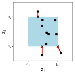
Figure 1: Example of the weight function in Equation 9 and the chaining function in Equation 11. Ten two-dimensional observations are shown before (points) and after (crosses) applying the chaining function. The shaded region is the area specified by the weight function. Points in this region are unchanged after applying the chaining function, whereas points outside of this region are mapped onto the region’s border, as indicated by the red arrows.

Similarly, for the smooth weight functions based on multivariate Gaussian distribution and density functions, a chaining function can be derived from a component-wise extension of the chaining functions corresponding to univariate Gaussian weight functions. Examples of such chaining functions are presented in Table 1. Note, however, that these component-wise extensions implicitly assume that the covariance matrix in the multivariate Gaussian weight function is diagonal. Readers are referred to AllenEtAl2022 for a more detailed discussion on multivariate chaining functions.

Although the weight and chaining functions presented in this section are simple examples that are frequently used in practice, the weighted scoring rules discussed herein can be employed with arbitrary such functions, permitting very flexible, user-oriented forecast evaluation. In the remainder of this paper, we will discuss how these weighted scoring rules have been integrated into the scoringRules package, facilitating their use in practical applications.

3 Package functionality

3.1 Univariate weighted scoring rules

The weighted scoring rules discussed in the previous section can all be implemented using the scoringRules package. Functionality is currently available for probabilistic forecasts that take the form of a predictive sample. In this case, it is straightforward to calculate the weighted scoring rules with arbitrary, user-specified weight functions, which is generally not the case for parametric families of distributions. Expressions for the weighted scoring rules discussed in the previous section when the forecast is a predictive sample are given in Appendix LABEL:app:sampleformulas.

The scoringRules package already contains functions to calculate the LogS, CRPS, ES, VS, and MMDS for forecasts in the form of predictive samples. Suppose the sample is comprised of $m$ members. As explained in JordanEtAl2018, the naming convention of these functions is [score]_sample(), where [score] refers to the scoring rule to be calculated. These functions take the observed value(s) and the forecast samples as inputs, and output the desired score value. For example, to calculate the CRPS corresponding to a vector of $n$ observations y and a $n\times m$ matrix dat whose rows contain the $m$ forecast samples corresponding to each observation, one could use crps_sample(y, dat) The output is a numeric vector containing the score for each of the $n$ forecast cases.

The same convention is adopted for the weighted scoring rules. In the univariate case, the following functions calculate the outcome-weighted and threshold-weighted CRPS, and the conditional or censored likelihood scores: owcrps_sample(y, dat, a = -Inf, b = Inf, weight_func = function(x) as.numeric(x > a & x < b), w = NULL, show_messages = TRUE) twcrps_sample(y, dat, a = -Inf, b = Inf, chain_func = function(x) pmin(pmax(x, a), b), w = NULL, show_messages = TRUE) clogs_sample(y, dat, a = -Inf, b = Inf, bw = NULL, show_messages = FALSE, cens = TRUE) The cens argument in clogs_sample specifies whether the conditional likelihood score or the censored likelihood score should be returned; the default is cens = TRUE, in which case the CeLS is calculated.

As discussed in Section 2.1, the LogS takes a predictive density as input, and hence cannot readily be applied to predictive samples. To circumvent this, logs_sample employs kernel density estimation to estimate a predictive density from the sample, and then calculates the LogS from the estimated density function. However, KruegerEtAl2021 demonstrate that the resulting score is sensitive to the bandwidth parameter bw of the kernel density estimation, and the authors therefore recommended using the CRPS instead of the LogS, particularly when the sample size $m$ is small. Similarly, the conditional and censored likelihood scores also require a predictive density as inputs, and kernel density estimation is used to estimate this from the predictive sample prior to calculating the weighted scores. We anticipate that these weighted scores will be yet more sensitive to the kernel density estimation parameters, especially when a weight function is used that targets more extreme outcomes. As such, when the forecast is in the form of a predictive sample, we similarly recommend employing weighted versions of the CRPS, rather than the conditional or censored likelihood score.

In addition to observations and forecast samples, the functions listed above have arguments that allow particular outcomes to be targeted when calculating the weighted scores. By default, the weighted scoring rules employ the weight function $w(z)=\mathbbm{1}\{a<z<b\}$, which, as discussed in the previous section, is most commonly applied in practice. The arguments a and b are single numeric values representing the lower and upper bounds in this weight function, respectively. If these arguments are not specified, then their default values are a = -Inf and b = Inf, resulting in a weight function that is always one, and thus recovering the unweighted scoring rules.

R> obs <- rnorm(5) R> sample_m <- matrix(rnorm(5e4), nrow = 5) R> score_df <- data.frame(crps = crps_sample(obs, sample_m), + owcrps = owcrps_sample(obs, sample_m), + twcrps = twcrps_sample(obs, sample_m)) R> print(score_df) crps owcrps twcrps 1 0.275 0.275 0.275 2 1.230 1.230 1.230 3 0.246 0.246 0.246 4 0.764 0.764 0.764 5 1.355 1.355 1.355

On the other hand, if we want to emphasise outcomes above a threshold t, then we can set the lower bound in the weight function to a = t, and the upper bound to b = Inf.

R> t <- 0 R> score_df <- data.frame(crps = crps_sample(obs, sample_m), + owcrps = owcrps_sample(obs, sample_m, a = t), + twcrps = twcrps_sample(obs, sample_m, a = t)) R> print(score_df) crps owcrps twcrps 1 0.275 0.000 0.120 2 1.230 0.000 0.115 3 0.246 0.000 0.119 4 0.764 0.306 0.645 5 1.355 0.809 1.235

Similarly, if we want to emphasise values below the threshold, then we can set a = -Inf and b = t. To avoid misuse, an error is returned if a is not smaller than b.

A useful diagnostic tool is to plot the average score as a function of the threshold. In this case, as the lower bound in the weight function a becomes smaller (or the upper bound b becomes larger), the weighted score tends to the unweighted score, allowing the user to simultaneously visualise overall forecast performance, as well as performance when predicting particular outcomes (GneitingRanjan2011). An example of this is presented in Figure 2, where the outcome-weighted CRPS and threshold-weighted CRPS for two forecasts distributions are displayed as a function of a in the default weight function, with b = Inf.

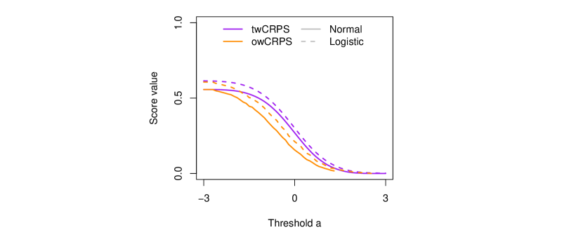
Figure 2: Average twCRPS (purple) and owCRPS (orange) as a function of the threshold $a$ in the weight function $w(z)=\mathbbm{1}\{z>a\}$. The observations are drawn from a standard normal distribution, and scores are shown for predictive samples from a standard normal (solid) and standard logistic (dashed) distribution. Note that for high thresholds, the owCRPS is not always well-defined.

3.2 Multivariate weighted scoring rules

Similarly to the LogS and CRPS, scoringRules contains functions to calculate the ES, VS, and MMDS for multivariate forecast distributions in the form of predictive samples. es_sample(y, dat, w = NULL) vs_sample(y, dat, w = NULL, w_vs = NULL, p = 0.5) mmds_sample(y, dat, w = NULL)

These multivariate scoring rule functions can only evaluate a single multivariate forecast at a time. Hence, the observation argument y is a vector of length $d$, representing an element in $\mathbb{R}^{d}$, the forecast argument dat is a $d\times m$ matrix, with the columns representing the simulated samples (or ensemble members) from the multivariate forecast distribution, and the output is a single value. These functions can then be sequentially applied to multiple forecast cases using the apply() functions or for loops (see Appendix B of JordanEtAl2018).

Similarly, outcome-weighted and threshold-weighted versions of these multivariate scoring rules are calculated using owes_sample(y, dat, a = -Inf, b = Inf, weight_func = function(x) as.numeric(all(x > a & x < b)), w = NULL) owvs_sample(y, dat, a = -Inf, b = Inf, weight_func = function(x) as.numeric(all(x > a x < b)), w = NULL, w_vs = NULL, p = 0.5) owmmds_sample(y, dat, a = -Inf, b = Inf, weight_func = function(x) as.numeric(all(x > a x < b)), w = NULL) twes_sample(y, dat, a = -Inf, b = Inf, chain_func = function(x) pmin(pmax(x, a), b), w = NULL) twvs_sample(y, dat, a = -Inf, b = Inf, chain_func = function(x) pmin(pmax(x, a), b), w = NULL, w_vs = NULL, p = 0.5) twmmds_sample(y, dat, a = -Inf, b = Inf, chain_func = function(x) pmin(pmax(x, a), b), w = NULL)

As in the univariate case, the default weight function corresponds to Equation 9, where interest is on a range of values in each dimension. The default chaining function used to calculate the threshold-weighted scores is Equation 11. Arguments a and b are again used to define the lower and upper bounds of the default weight function. In contrast to the univariate case, however, a and b are numeric vectors of length $d$, rather than single values.

If the input value of a or b is a single value, then it is automatically converted into a vector of length $d$, all containing the same element. The default values are a = -Inf and b = Inf, which again returns the unweighted scoring rule. Hence, if we want to emphasise values above the same threshold $t$ in all dimensions, then we could either use a = c(t, t, …) and b = c(Inf, Inf, …), or we could use a = t and b = Inf. For example, for the threshold-weighted energy score, we have R> d <- length(obs) R> twes_sample(obs, sample_m, a = t) [1] 1.34 R> twes_sample(obs, sample_m, a = rep(t, d)) [1] 1.34

Finally, note that the functions to calculate the multivariate weighted scores also include optional weight arguments that cannot be used to target particular outcomes of interest. The argument w is a vector of length $m$ that allows more weight to be given to particular elements of the sample in the forecast distribution. This argument is also available when calculating the unweighted scoring rules, and the univariate weighted scores. The variogram score functions additionally have an argument w_vs, which is a $d\times d$ matrix containing the scaling parameters $h_{i,j}$ in Equation 4. These scaling parameters put more emphasis on combinations of dimensions of the multivariate variables, rather than targeting particular outcomes.

3.3 Custom weight and chaining functions

The functions to calculate the weighted scoring rules use a default weight function that assumes emphasis is to be placed on a particular region of the outcome space. Although this weight function is frequently applied in practice, it may be the case that another weight function is desired. As discussed, the motivation for considering only forecasts in the form of a predictive sample is that it is straightforward to calculate the resulting scores for arbitrary weight and chaining functions. The weighted scoring rule functions in scoringRules therefore additionally contain an argument that allows for a custom weight or chaining function to be used.

The weight_func argument can be used to incorporate a custom weight function into the outcome-weighted scoring rules. This argument must be a function that takes a vector as an input, and outputs either a vector of the same length as the input (if a univariate scoring rule is being used), or a single numeric value (if a multivariate scoring rule is used). An error is returned if the weight function is found to return negative weights, or if the output is not of the correct format.

For example, consider the Gaussian distribution function in Equation 8, with location parameter mu and scale parameter sigma. To use this as the weight function when calculating the outcome-weighted CRPS, one could use

R> mu <- 0; sigma <- 1 R> weight_func <- function(x) pnorm(x, mean = mu, sd = sigma) R> owcrps_sample(obs, sample_m, weight_func = weight_func) [1] 0.2002 0.0703 0.1868 0.3524 0.8788

Similarly, a multivariate Gaussian distribution could be used as a multivariate weight function. Let mu be the mean vector of this distribution, and assume the covariance matrix is diagonal with entries $\sigma_{1},\dots,\sigma_{d}$. Then, the outcome-weighted ES with this weight function can be calculated using

R> mu <- rnorm(d, 0, 0.5); sigma <- runif(d, 0.5, 1.5) R> weight_func <- function(x) prod(pnorm(x, mean = mu, sd = sigma)) R> owes_sample(obs, sample_m, weight_func = weight_func) [1] 0.0418

Whereas the outcome-weighted scores depend on a weight function, the threshold-weighted scores rely on a chaining function. For the threshold-weighted CRPS, a chaining function corresponds directly to a weight function via Equation 10. However, computation of the threshold-weighted CRPS for a sample forecast requires the chaining function rather than a weight function, and hence functionality is not currently available to take a weight function as an argument. In this case, it is necessary to derive the chaining function corresponding to the weight. For the simple weight functions commonly used in practice, this is typically straightforward to achieve (see Table 1 for popular choices).

The chain_func argument can be used to incorporate a custom chaining function into the threshold-weighted scoring rules. In contrast to weight_func, the chain_func argument should be a function whose inputs and outputs are the same length as the observation input y. For example, in the multivariate case, this function should both input and output a vector of length $d$.

In the univariate case, if the chaining function satisfies Equation 10 for some non-negative weight function $w$, then it will be a non-decreasing function; that is, if $z>z^{\prime}$, then $v(z)\geq v(z^{\prime})$ for all $z,z^{\prime}\in\mathbb{R}$. While a decreasing chaining function could also be used within Equation 2, this does not correspond to the original definition of the twCRPS presented in GneitingRanjan2011, and is therefore not recommended: a warning message is returned if chain_func is found to be decreasing.

Table 1 contains possible chaining functions corresponding to the Gaussian weight functions employed above. These chaining functions can be implemented within twcrps_sample and twes_sample as follows

R> chain_func <- function(x) (x - mu)*pnorm(x, mu, sigma) + + (sigma^2)*dnorm(x, mu, sigma) R> mu <- 0; sigma <- 1 R> twcrps_sample(obs, sample