IMSc/2023/03
Impact of errors in the magnetic field measurement on the precision determination of neutrino oscillation parameters at the proposed ICAL detector at INO

Abstract

The magnetised iron calorimeter (ICAL) detector proposed at the India-based Neutrino Observatory will be a 51 kton detector made up of 151 layers of 56 mm thick soft iron with 40 mm air gap in between where the RPCs, the active detectors, will be placed. The main goal of ICAL is to make precision measurements of the neutrino oscillation parameters using the atmospheric neutrinos as source. The charged current interactions of the atmospheric muon neutrinos and anti-neutrinos in the detector produce charged muons. The magnetic field, with a maximum value of $\sim$ 1.5 T in the central region of ICAL, is a critical component since it will be used to distinguish the charges and determine the momentum and direction of these muons. It is difficult to measure the magnetic field inside the iron. The existing methods can only estimate the internal field and hence will be prone to error. This paper presents the first simulations study of the effect of errors in the measurement of the magnetic field in ICAL on its physics potential, especially the neutrino mass ordering and precision measurement of oscillation parameters in the 2–3 sector. The study is a GEANT4-based analysis, using measurements of the magnetic field at the prototype ICAL detector. We find that there is only a small effect on the determination of the mass ordering. While local fluctuations in the magnetic field measurement are well-tolerated, calibration errors must remain well within 5% to retain good precision determination of the parameters $\sin^{2}\theta_{23}$ and $\Delta m^{2}_{32}$.

1 Introduction

The proposed magnetised Iron Calorimeter (ICAL) detector at the India-based Neutrino Observatory (INO) [1] is primarily designed as an atmospheric neutrino detector. Its main goal is to detect muons produced in the charged current (CC) interactions of atmospheric muon neutrinos (and anti-neutrinos) with the detector, via

$$\nu_{\mu}N\to\mu^{-}X~{};\hskip 28.45274pt\overline{\nu}_{\mu}N\to\mu^{+}X~{}.$$ (1)

The magnetic field will determine the sign of the charge of the muons (through the bending of the charged particle tracks in the detector) and hence be able to distinguish neutrino- and anti-neutrino-initiated events. This key feature will enable a clean determination of the as-yet unknown sign of the neutrino mass ordering and hence the neutrino mass hierarchy. A precise determination of the magnetic field map over the entire ICAL detector is therefore a crucial input in this determination. The ICAL detector will also make precision measurements of the 2–3 neutrino oscillation parameters such as $\sin^{2}\theta_{23}$ and $\Delta m^{2}_{32}$; both these also depend on correctly determining the muon momenta using the knowledge of the magnetic field map. In this paper, we present for the first time, a detailed simulations study of the impact of measurement errors in the magnetic field on the physics potential of the ICAL detector.

The paper is organised as follows: we present a short summary of the current status of neutrino oscillation physics in Section 2. In Section 3, we present some highlights of the proposed ICAL detector. We also present a summary of the magnetic field measurements made in the prototype mini-ICAL detector, an 85 ton scale model, that has been functioning for the last few years. We will use these results, especially, the measured errors in both calibration and measurement of the magnetic field, in Section 5, to analyse the impact of these errors on the precision measurement of the neutrino oscillation parameters. Before doing this, we first present in Section 4 a detailed simulations study of the effect of errors—in calibration and in measurement—of the magnetic field map on the reconstruction of the muon momenta and compare it with older results where the magnetic field was assumed to be well-defined [3]. We use these results to parametrise the changes in the reconstruction values (central value, spread, etc), with respect to fixed changes in the magnetic field. We present our results in Section 6 and We conclude with a discussion of the results in Section 7.

2 Neutrino oscillation: summary and status

In 1968 Pontecorvo [4] proposed the quantum mechanical phenomenon of neutrino oscilaations in analogy with K⁰ and $\overline{K^{0}}$ oscillations. In 1962 Maki, Nakagawa and Sakata [5] for the first time constructed a model with mixing of different neutrino flavors. Currently, the three neutrino flavours, $\nu_{e},\nu_{\mu},\nu_{\tau}$, can be expressed in terms of the mass eigen states, $\nu_{1},\nu_{2},\nu_{3}$, using three mixing angles $\theta_{12}$, $\theta_{23}$ and the across-generation mixing angle, $\theta_{13}$, as well as a CP-violating phase for Dirac-type neutrinos, $\delta_{CP}$. Non-zero and different neutrino mass-squared differences, $\Delta m_{ij}^{2}\equiv m_{i}^{2}-m_{j}^{2}$, with $i,j=1,2,3$ along with mixing lead to neutrino oscillations which have since been observed in solar, atmospheric, reactor, and accelerator neutrinos.

2.1 Neutrino experiments

The first solar neutrino experiment were detected by Ray Davis and his collaborators in the Homestake experiment using Chlorine as the active detector material. Neutrino oscillation could account for the fact that the measured rate of charged current interactions of electron-type neutrinos was one third of the rate predicted by the solar standard model. This was followed by Kamiokande and Super Kamiokande experiments with water Cerenkov detectors in Japan, and lastly by the Sudbury Neutrino Observatory in Canada which observed the solar neutrinos in both the charged and neutral current (NC) channels and confirmed the phenomenon of neutrino oscillations and non-zero neutrino masses in the solar (primarily 1–2) sector. The anomaly between the atmospheric electron and muon neutrino measurements of the Super Kamiokande experiment could also be resolved within the neutrino oscillation paradigm.

Subsequently, T2K long baseline neutrino experiment, the LSND experiment, the Daya Bay reactor (anti-)neutrino experiment, the MiniBoone experiment, the MINOS long baseline experiment and the Ice Cube experiment at the South pole have all confirmed neutrino oscillations in different flavours and sectors. While the solar and reactor neutrino sector mainly determines the parameters in the 1–2 sector, atmospheric and accelerator experiments have been used to pin down the parameters of the 2–3 sector. In particular, the reactor experiments have played a crucial role in determining the non-zero though small value of $\theta_{13}$. While it has been established that $\Delta m^{2}_{21}>0$, the mass ordering in the 2–3 sector, viz., the sign of the mass squared difference $\Delta m^{2}_{32}$ (or equivalently, of $\Delta m^{2}_{31}$), is currently not known. In addition, the value of the CP phase as well as the octant of the mixing angle $\theta_{23}$ is not yet established. The up-coming DUNE [6] and JUNO [7] experiments will also probe these parameters. The current status of neutrino oscillation mixing parameters can be found in Refs. [8, 9]; the best-fit values and their $3\sigma$ ranges (which we use in this analysis) are shown in Table 1.

For convenience, we define [10]

$$\Delta m^{2}\equiv m_{3}^{2}-\left(\frac{m_{2}^{2}+m_{1}^{2}}{2}\right)~{}.$$ (2)

Note that $\Delta m^{2}$ flips sign without changing its magnitude when the hierarchy/ordering changes and hence is a convenient parameter compared to $\Delta m_{31}^{2}$ or $\Delta m_{32}^{2}$, which change in both sign and magnitude depending on the mass ordering. We shall use $\Delta m^{2}$ throughout in the analysis. Depending on the mass ordering, and using the value of $\Delta m_{21}^{2}$ given in Table 1, the values of $\Delta m_{31}^{2}$ and $\Delta m_{32}^{2}$ can be found from $\Delta m^{2}$. We shall assume the normal ordering throughout this analysis, unless otherwise specified.

Parameter	Central values	$3\sigma$ Range
$\sin^{2}\theta_{12}$	$0.304$	fixed
$\sin^{2}\theta_{13}$	$0.0222$	$0.0203\leftrightarrow 0.0241$
$\sin^{2}\theta_{23}$	$0.5$	$0.381\leftrightarrow 0.615$
$\Delta m^{2}_{21}$ $(\times 10^{-5}$ eV2)	$7.42$	fixed
$|\Delta m^{2}|$ $(\times 10^{-3}$ eV2)	$2.47$	$2.395\leftrightarrow 2.564$
$\delta_{CP}(^{\circ})$	$0.0$	fixed

Table 1: The $3\sigma$ ranges of neutrino oscillation parameters — mixing angles and mass squared differences — and central values used in the present work [8, 9]; $\Delta m^{2}$ is defined in Eq. 2.

3 Highlights of the ICAL detector

There are two sources of muon neutrinos (and anti-neutrinos) from Earth’s atmosphere. One are those muon neutrinos produced from decays of secondary pions via $\pi\to\mu\nu_{\mu}$ with the subsequent decay of the muons into additional muon neutrinos via $\mu\to\nu_{\mu}e\nu_{e}$. Due to the presence of neutrino oscillations, it is also possible to detect muon neutrinos, which have been produced through oscillation of electron neutrinos on their way to the detector. Typically, neutrinos arriving from below (so-called up-going neutrinos, produced in the atmosphere on the other side of the Earth) are more likely to exhibit oscillations due to the relevant GeV-scale energies and path-lengths involved. Hence there will be two contributions to the detected muons arising from CC interactions in ICAL: those produced by muon neutrinos that have survived during their journey, involving the neutrino survival probability $P_{\mu\mu}$ and those produced by electron neutrinos that have oscillated into muon neutrinos, involving the oscillation probability $P_{e\mu}$. These probabilities depend on both the neutrino energy and path-length travelled; depending on the neutrino mass ordering, these show MSW enhancement [11, 12] in the few-GeV energy range for neutrinos passing through Earth matter with path lengths such that the zenith angle is less than $\theta<45^{\circ}$ (with $\cos\theta=1$ for vertically upward neutrinos). Specifically, the resonance will be visible in the neutrino sector for normal ordering with $\Delta m^{2}>0$ and in the anti-neutrino sector for inverted ordering with $\Delta m^{2}<0$.

3.1 The ICAL detector

The proposed ICAL (Iron Calorimeter) detector is a 51 kton magnetised detector to be located at the India-based Neutrino Observatory (INO) with a rock cover of at least 1 km in all directions. It will consist of three modules of size 16 m $\times$ 16 m $\times$ 14.5 m in ($x$, $y$, $z$ dimensions) consisting of 150 layers of resistive plate chamber (RPC) which will act as an active detector to detect muons and 151 layers of 56 mm thick iron plates which will act as interaction material for neutrinos. There will be a 40 mm gap between each two iron layers to place the RPC in between. There will be three sets of current carrying copper coils which will be energised to produce the required magnetic field in the detector.

ICAL is designed to detect muons of energy range from 1–25 GeV generated from the CC interactions of the atmospheric $\nu_{\mu}$ and $\overline{\nu}_{\mu}$ neutrinos. One of the special features of ICAL is that it is sensitive to the charge of muons because of the presence of magnetic field of B_max $\sim$ 1.5 Tesla. While the field is mainly in the $y$ direction in the central region (see Fig. 1) and in the side region, although smaller by about 15%, it varies in both magnitude and direction in the peripheral region. The map has been generated [13] using the MAGNET6 [14] software and has been extensively used in all simulations analyses of ICAL [1].

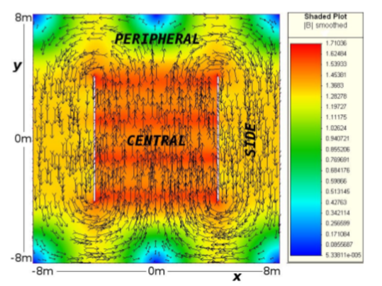
Figure 1: Field map of simulated magnetic field for ICAL detector from Ref. [13]; shown is the field in the $x$–$y$ plane in the centre of a single iron layer. The field is uniform in the $z$ direction over the thickness of the iron.

Each RPC has pick-up strips along the $x$- and $y$-directions respectively above and below, so that whenever a charged particle passes through it, signals will be collected as “hits” for that layer independently in both the $x$ and $y$ directions. As the muon bends in the magnetic field depending on the sign of its charge, the bending of the track along with information on the magnetic field in the region is used by a Kalman Filter program to reconstruct the muon momentum (magnitude and direction) as well as the sign of its charge, depending on whether it is up-coming or down-going; this latter is determined based on the timing information which is available to an accuracy of about 1 ns. We will present results on the muon reconstruction efficiencies and energy resolutions in a later section. We will first present details of the measurement of the magnetic field at the prototype mini-ICAL detector and how we use it as an input in the current analysis.

3.2 Experimental inputs from mini-ICAL

The mini-ICAL is a fully functional prototype detector working at the transit campus of INO near Madurai in Tamil Nadu, India. It was built to study the challenges and difficulties that could be faced while installing the main ICAL detector. It is an 85 ton detector which consists of 11 layers of 56 mm thick iron and 10 layers of RPCs which are sandwiched between the iron layers as active detector elements. Each iron layer is made up of 7 plates with an overall dimension of $4\times 4$ m²; see Fig. 2. The two sets of copper coils each having 18 turns are used to magnetize mini-ICAL by flowing current through the coils.

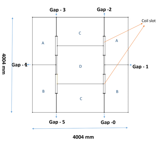
Figure 2: Schematic of top view of mini-ICAL showing the gaps between plates in a layer.

The mini-ICAL detector has been constructed with 3 mm gaps built-in on purpose between the different iron plates in layers 1, 6, and 11 (top, middle and bottom); see Fig. 2, in order to enable the measurement of the magnetic field in the gaps using a Hall probe. A detailed study of the magnetic field all along the gaps from a location near the coil slots to the outer edges of the detector, and in the air just outside, has been made [15]. Separately, a detailed simulations study of the magnetic field in mini-ICAL [16] as a function of the coil current and the gap widths, has been made using the MAGNET6 software [14]. As expected, the magnetic field was more or less uniform and largest in magnitude in the central region, with $|x|,|y|\leq 1$ m between the coil slots. (Note that the origin is defined to be the centre of the detector). The field is somewhat smaller and in the opposite direction in the side region outside the slots, $|x|\geq 1$ m; $|y|\leq 1$ m, while the field is changing in both magnitude and direction in the peripheral region with $|y|\geq 1$m. In particular, in the peripheral region, the field is largest near the coil slot and decreases toward the outside. Also, as expected, the field is smaller when the gap width is larger; see Fig. 3. Hence the field in the mini-ICAL is similar to that expected from simulations on the main ICAL detector. In addition, it was found [15]. that the magnetic field in mini-ICAL can be measured to within an accuracy of 3% [15].

A comparison of the measured and simulated field at mini-ICAL indicated that it may be possible to get agreement between measured and simulated field values to within about 10%. When the difference between the measured and simulated gap widths was taken into account, the agreement improves to within 5%. In this paper, we use the results of this study and assume a similar result will hold for the main ICAL detector; i.e., we use the magnetic field map for the entire ICAL detector as simulated by the MAGNET6 software. Assuming that errors on this do not exceed about 5%, we present a preliminary and first study of the effect of errors in the measurement of the magnetic fields on the physics goals of ICAL.

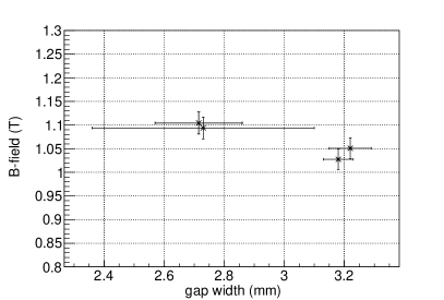
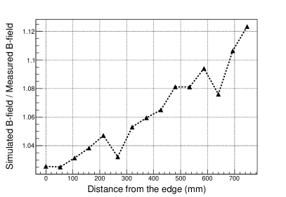
Figure 3: Left: Variation of magnetic field as a function of the gap width in mini-ICAL, from Ref.  [15]. Right: Ratio of simulated [16] to measured magnetic field in gap 0 of mini-ICAL as a function of the distance from the edge of the detector. The right-most values are close to the coil gap.

We use these values in our simulations study of muons in the main ICAL detector, with true and modified magnetic fields.

4 Simulations Study of Muons

The GEANT4 [17] code is used to generate the ICAL geometry which comprises three modules of 151 layers of 56 mm iron, separated by a 40 mm gap in which the active detector elements, the RPCs, are inserted. The magnetic field map shown for a single iron layer in Fig. 1 is generated using MAGNET 6.0 software [1]. The calibration of muon energy/momentum is done analogous to the approach discussed in detail in Refs. [3, 18]. Here, 10,000 muons of fixed energy and direction $(p_{\mu},cos\theta)$ are generated at random over the entire detector and propagated in the ICAL detector using the magnetic field map shown in Fig. 1; henceforth this is called the “true” magnetic field, $B(x,y,z)$. The charged particles, on passing through the RPCs, trigger a discharge, which is acquired as a “hit” in the detector. The collection of hits through different layers forms a track. The magnetic field bends the muons into the observed muon track. The hit pattern is studied and the reconstruction of the various muon properties is done using a Kalman filter algorithm which requires hits in at least 5 consecutive layers. The algorithm identifies the hits which are a part of the muon track (non-trivial in the case of a genuine neutrino charged-current (CC) event with associated hadron hits), and returns the direction $(\cos\theta,\phi)$, the magnitude of the momentum and the sign of the charge of the muon. Various selection criteria are used [3, 18] to improve the fit quality. The histogram of reconstructed momenta is fitted to a gaussian which returns the mean reconstructed momentum/energy ($E_{reco}(p_{\mu},\cos\theta)$) and width ($\sigma(p_{\mu},\cos\theta)$) as a function of the true input values. The number of reconstructed events to the total number is the reconstruction efficiency, $\epsilon_{reco}$, also a function of the input energy/momentum and direction, and the relative number of correctly charge identified tracks to the number reconstructed is the relative charge identification efficiency, $\epsilon_{cid}$. This analysis was performed for sets of muons with energies 1–25 GeV in steps of 1 GeV, and with zenith angle $\cos\theta=0.3$–0.9 in steps of 0.1. Details of the quality of these fits, etc., can be found in the references given earlier.

4.1 Parametrisation with modified magnetic fields

We wish to study the response of the detector when the measured magnetic field is different from the true one. In order to be able to parametrise the effect of such errors, and to quantify them, we use the following approach.

The same muon tracks are now fitted and reconstructed with a computed or simulated magnetic field map which is different from the actual one. For simplicity, 6 scenarios, when the fitted magnetic field is systematically different from the true value by a constant factor, $B_{reco}=fB$, are considered, viz., the fields are taken to be $B_{meas}=0.7B,0.8B,0.95B,1.05B,1.2B,1.30B$, so $f=0.7,0.8,0.95,1.05,1.2,1.3$, that is, magnetic fields which are 30%, 20$\%$, or 5$\%$ smaller or larger than the true magnetic field as given by the magnetic field map. The reconstructed energy $E_{reco}$, the energy resolution $\sigma$, and the reconstruction and charge identification efficiencies are calculated in each case. Fig. 4 shows the reconstructed muon energy as a function of the true value over the relevant range for atmospheric neutrinos from 1–25 GeV. In the interests of clarity, only every 5th energy value is plotted for angles $\cos\theta=0.4,0.6,0.8$ (closely overlapping points with the smallest value corresponding to the smallest $\cos\theta$). It can be seen that the reconstructed energy $E_{reco}^{fB}$ increases (decreases) for a given true value $E_{true}$ as $f$ increases (decreases). The results for $f=0.8,1.2$ only are plotted in comparison to the true value ($f=1$), again for clarity.

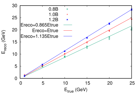
Figure 4: Reconstructed muon energy E_reco vs E_true for cos$\theta$ = 0.4, 0.6 and 0.8 using a magnetic field which is 0.8, 1.0 and 1.2 times the true magnetic field map.

It turns out that E${}^{fB}_{reco}$ is given to a very good accuracy by a constant scale parameter compared to E${}^{B}_{reco}$ for the original map, where $f$ = 0.8, 0.95, 1.05, 1.2, etc. The actual reconstructed values (for $\cos\theta=0.8$) are shown along with this fit in Fig. 4 as a function of E_true. For larger deviation from the true magnetic field ($\sim$20 %), it can be seen from Fig. 5 that there is a non-linear variation of the reconstructed energy; the results fit marginally better to a quadratic, but for smaller deviations (upto 5%) the fit is almost linear for all the three mentioned regions (I, II and III), and therefore the change can be parametrised by fitting with a straight line. This is shown in Table 2.

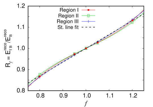
Figure 5: The ratio $R_{f}$ of the reconstructed muon energies when the modified and true magnetic field maps respectively are used, as a function of the modification parameter, $f$. The results are similar for the three different regions, central (I), side (II), and peripheral (III), as explained in the text. The ratio is almost linear for smaller values of $|1-f|$.

B-field	f	$E_{reco}$ vs $E_{true}$
$B=B_{true}$	1.00	$E_{reco}\sim E_{true}$
$B=0.8B_{true}$	0.80	$E_{reco}=0.865E_{true}$
$B=0.95B_{true}$	0.98	$E_{reco}=0.965E_{true}$
$B=1.05B_{true}$	1.02	$E_{reco}=1.035E_{true}$
$B=1.2B_{true}$	1.20	$E_{reco}=1.135E_{true}$

Table 2: Change in the energy reconstruction (E_reco) of muon w.r.t. change in the magnetic field by a constant factor $f$ across the entire map.

In addition the width and hence the energy resolution for muons varies as $\sigma(fB)=f\sigma(B)$. The angular resolution, the reconstruction and charge identification efficiencies are practically independent of the choice of magnetic field map, except at very low energies, $E_{\mu}\leq 2$ GeV. In this first, rather simplistic analysis, we ignore these outliers and take these values to be the same as with the true magnetic field. Obviously, the hadron energy resolution (fitted to the number of hadron hits; see Ref. [19] for details) is also independent of the choice of the magnetic field map.

With this analysis, we are now ready to analyse the impact of magnetic field measurement errors on the physics reach of ICAL from charged current (CC) interactions of atmospheric neutrinos in the detector. Throughout we use the baseline results from Ref. [20, 10] for comparison.

5 Simulations study of impact of errors in magnetic field measurement at ICAL

5.1 Events generation

Both $\nu_{e}$ and $\nu_{\mu}$ types of neutrinos (and their anti-particles) are present in atmospheric neutrino fluxes (the direct tau-neutrino contribution is negligible at these energies and are only produced through oscillation). Charged current (CC) atmospheric neutrino (and anti-neutrino) events were simulated for an exposure of 1000 years at the ICAL detector using the NUANCE neutrino generator [21] and Honda 3-D fluxes [22]. The “data” is generated using the current central best fit values of various neutrino oscillation parameters as listed in Table 1 which are considered to be the “true” values. Note that the analysis is completely insensitiveto the CP phase $\delta_{CP}$ and we have assumed maximum mixing in the 2–3 sector, viz., $\theta_{23}=45^{\circ};\sin^{2}\theta_{23}=0.5$ throughout. In addition, normal ordering is assumed unless otherwise specified.

Since the “theory” events are to be generated with different values of these oscillation parameters, the NUANCE events were generated without oscillations, which were applied event-by-event later. The rate of observed charged muons of either type in the detector in terms of the true final state muon energy and direction is given by

$$\frac{{\rm d}^{2}N_{\mu}}{{\rm d}E_{\mu}{\rm d}\cos\theta_{\mu}} = T\times N_{D}\times\int{\rm d}E_{\nu}{\rm d}\cos\theta_{\nu}{\rm d}\phi_{\nu}\left[P_{\mu\mu}\frac{{\rm d}^{3}\Phi_{\mu}}{{\rm d}E_{\nu}{\rm d}\cos\theta_{\nu}d\phi_{\nu}}+\right.$$ (3)

$$\left.P_{e\mu}\frac{{\rm d}^{3}\Phi_{e}}{{\rm d}E_{\nu}{\rm d}\cos\theta_{\nu}{\rm d}\phi_{\nu}}\right]\times\frac{{\rm d}^{2}\sigma^{CC}_{\mu}}{{\rm d}E_{\mu}{\rm d}\cos\theta_{\mu}}~{},$$

where $T$ is the exposure time in seconds, $N_{D}$ is the number of target nuclei, $\Phi_{e,\mu}$ are the electron and muon type atmospheric neutrino fluxes, and $\sigma^{CC}_{\mu}$ is the charged current cross section for the muon neutrino interaction in the detector. Here $P_{\mu\mu}(E_{\nu},\cos\theta_{\nu})$ is the muon neutrino survival probability and $P_{e\mu}(E_{\nu},\cos\theta_{\nu})$ is the oscillation probability of electron neutrino into muon neutrino. For anti-neutrinos, the corresponding anti-neutrino fluxes, cross sections and probabilities are used. It is seen that both $\nu_{\mu}$ and $\nu_{e}$ fluxes contribute (the former through the survival probability $P_{\mu\mu}$ and the latter through the oscillation probability $P_{e\mu}$). Hence events using both sets of initial fluxes were generated.

Symbolically, the true number of oscillated events can be expressed as

$$N_{\mu^{-}} = N_{\mu^{-}}^{0}\times P_{\mu\mu}+N_{e^{-}}^{0}\times P_{e\mu}~{},$$ (4)

$$N_{\mu^{+}} = N_{\mu^{+}}^{0}\times\overline{P}_{\mu\mu}+N_{e^{+}}^{0}\times\overline{P}_{e\mu}~{}.$$

That is, the events N${}^{0}_{\mu\pm}$ were generated by using the $\nu_{\mu}$ fluxes and the events N${}^{0}_{e\pm}$ were generated by swapping the $\nu_{\mu}$ and $\nu_{e}$ fluxes in the generator, retaining the same cross sections.

The above equations, Eq. 5.1, are just representative in order to understand the different contributions. Actually, the events are generated by NUANCE, so that $N^{0}_{\mu\pm}$ are the un-oscillated muon events and $N^{0}_{e\pm}$ are swapped muon events generated by NUANCE, and $N_{\mu^{\pm}}$ are generated from the $\overline{\nu}_{\mu}$ and $\nu_{\mu}$ events respectively by applying neutrino oscillations. At the end of the events generation, we have events listed in full detail, including the energy and direction $(E_{\nu},\cos\theta_{\nu},\phi_{\nu})$ of the initial neutrino, the energy and direction of the final state muon, $(E_{\mu},\cos\theta_{\mu},\phi_{\mu})$ along with the sign of its charge, and detailed information on all the final state hadrons produced in the interaction. As detailed in Ref. [20], we use the information on the muon energy and direction $(E_{\mu},\cos\theta_{\mu})$, and the total hadron energy, $E_{had}^{\prime}\equiv E_{\nu}-E_{\mu}$, for the analysis, while retaining the information on the neutrino energy and direction $(E_{\nu},\cos\theta_{\nu})$, for later use in order to generate the neutrino oscillation probabilities.

5.2 Inclusion of detector response

The events generated by the NUANCE neutrino generator give the true values of the various parameters. However, in the actual detector, these will be smeared depending on the detector resolutions. We therefore smear the events according to the detector response studied in the previous section. That is, we incorporate the efficiencies as well as the resolutions in both energy and direction. In particular, we use the look-up tables generated as described in the previous section to smear the values of the muon energy and direction, as well as the hadron energy, $(E_{\mu},\cos\theta_{\mu},E_{had}^{\prime})$. The binning of the events is done after including reconstruction efficiency of the muon and charge identification efficiency of the detector. The observed muon CC events are then given as

$$N^{tot}_{\mu^{-}}(E^{obs}_{\mu},\cos\theta^{obs}_{\mu},E_{had}^{{}^{\prime}obs}) = \epsilon_{rec}\epsilon_{cid}N_{\mu^{-}}+\epsilon_{rec}(1-\epsilon_{cid})N_{\mu^{+}}~{},$$ (5)

$$N^{tot}_{\mu^{+}}(E^{obs}_{\mu},\cos\theta^{obs}_{\mu},E_{had}^{{}^{\prime}obs}) = \epsilon_{rec}\epsilon_{cid}N_{\mu^{+}}+\epsilon_{rec}(1-\epsilon_{cid})N_{\mu^{-}}~{}.$$

Here $\epsilon_{rec}$ and $\epsilon_{cid}$ are the reconstruction efficiency and charge identification efficiency of the detector for both $\mu^{+}$ and $\mu^{-}$; N${}^{tot}_{\mu^{-}}$ and (N${}^{tot}_{\mu^{+}})$ are the total oscillated CC $\nu_{\mu}$ ($\overline{\nu}_{\mu}$) events that will be observed in a given $(E^{obs}_{\mu},\cos\theta^{obs}_{\mu},E_{had}^{{}^{\prime}obs})$ bin. Notice that since $\epsilon_{cid}<1$, a few $\mu^{+}$ events are mid-identified as $\mu^{-}$ events and vice versa. However, $\epsilon_{cid}>98$% for $E_{\mu}\gtrsim 2$ GeV; hence this contamination is small.

The “theory” events were smeared as per the resolutions corresponding to the incorrect magnetic field map by assuming the field to be $B_{reco}=fB_{map}$, where $f=0.95$, for instance. That is, the mean and $\sigma$ of the muon energy are calculated based on the value of $f$, as explained above. More details on the nature of the smearing are given below.

The events are oscillated using the oscillation parameters given in Table 1. The normal ordering is assumed throughout unless otherwise specified. The data was scaled to 10 years so all results correspond to 10 years exposure at ICAL.

5.3 Analysis

The main goal of this study is to understand the impact of errors in the magnetic field measurement in ICAL on the sensitivity to the neutrino oscillation parameters, especially in the 2–3 sector that atmospheric neutrinos are dependent on. We study the impact of two different kinds of errors. In both cases, events are generated according to the true magnetic field map as shown in Fig. 1. Hence the “data” that is to be fitted to “theory” is always generated according to the true map, as would be the case if there was real data from ICAL. For the “theory” events, there are two possibilities. One is that there was a calibration error so that the measured magnetic field is systematically higher or lower than the true one (which is represented by the original magnetic field map in this analysis). Also, it is possible that the local magnetic field where an event is generated is different from the simulated value due to fluctuations in iron quality, composition or deviations in the physical construction. The latter case is idealised by assuming that the local magnetic field fluctuates randomly around the “true” or map value. Hence we consider the following scenarios.

1. Considering the magnetic field map using the “true” $B$-field where the magnetic field that is generated using MAGNET software (see Fig. 1) is used to reconstruct the events. The results corresponding to use of the true map for both data generation and theory analysis are already available [1].

2. Considering the impact of a systematic change in the $B$-field map ($f=$ constant). Here the magnetic field is systematically increased or decreased constantly by a factor $f$ for the whole map and the “theory” events are reconstructed according to this modified map.

3. Considering random Gaussian variation in the $B$-field map. Here the local magnetic field where the event is generated via a random gaussian which is centred around the true value as given by the field map, with a width $\sigma=5$% about the central value. In this case the magnetic field value is ramdomly varied by generating a random number with the sigma 0.05 of the central value (true field value) of the field and the “theory” events are reconstructed using the corresponding generated field value, $fB$. The importance and usefulness of the linear parametrisation developed in the previous section is now obvious: the random gaussian number generates an arbitrary value of the scale factor $f$ and the reconstructed muon energy is calculated based on linear interpolation.

Of course, it is possible that the realistic case will correspond to inclusion of both systematic and measurement errors but we only consider them individually in this analysis.

5.4 $\chi^{2}$ analysis

Both the “data” and “theory” events are scaled to 10 years (unless otherwise specified) and binned in bins of observed muon energy and direction $(E_{\mu}^{obs},\cos\theta_{\mu}^{obs})$ and observed hadron energy, $E_{had}^{{}^{\prime}obs}$. The number and size of the bins were optimised in the earlier study [20] and used as-is in this analysis.

Apart from the specific magnetic field variation of interest, we consider five types of systematic errors which are given in Table 3 and which are included using the method of pulls. The flux normalization pull is the uncertainty in the assumed (theoretical) energy dependence of the atmospheric neutrino flux and it is calculated for each bin as follows:

$$\Phi_{\delta}(E)=\Phi_{0}(E)\left(\frac{E}{E_{0}}\right)^{\delta}\simeq\Phi_{0}(E)\left(1+\delta\ln\frac{E}{E_{0}}\right)~{}.$$ (6)

The uncertainty in angular flux is taken to be 5% cos$\theta$, that in the overall flux normalization is considered as 20%, the uncertainty in the cross section is considered to be 10% and an overall uncertainty in detector response is taken to be 5%.

Systematic error	Error
Flux normalization	20%
Shape uncertainty or tilt	5%
Zenith angle uncertainty	5%
Cross section uncertainty	10%
Detector response	5%

Table 3: The five types of systematic uncertainties included in the analysis.

The analysis closely follows that used in Ref. [20] and the results of that work will be used as a baseline to understand the effects of errors in the measurement of the magnetic field.

The loss of sensitivity due to using the incorrect field map during reconstruction of the “theory” events is determined through $\chi^{2}$ which is the sum of contributions from $\mu^{+}$ and $\mu^{-}$ observed events:

$$\chi^{2} = {\stackrel{{\scriptstyle[}}{{\displaystyle}}{\xi_{l}^{\pm}}]{}{\hbox{min}}}\sum^{N_{E^{obs}_{\mu}}}_{i=1}\sum^{N_{\cos\theta^{obs}_{\mu}}}_{j=1}\sum^{N_{E^{\prime obs}_{had}}}_{k=1}\left\{2\left[\left(T^{+}_{ijk}-D^{+}_{ijk}\right)-D^{+}_{ijk}\ln\left(\frac{T^{+}_{ijk}}{D^{+}_{ijk}}\right)\right]+\right.$$ (7)

$$\left.2\left[\left(T^{-}_{ijk}-D^{-}_{ijk}\right)-D^{-}_{ijk}\ln\left(\frac{T^{-}_{ijk}}{D^{-}_{ijk}}\right)\right]\right\}+\sum^{5}_{l^{+}=1}\xi^{2}_{l^{+}}+\sum^{5}_{l^{-}=1}\xi^{2}_{l^{-}}~{},$$

where T, D correspond to “theory” and “data”, with the former including the systematic errors through

$$T^{+}_{ijk} = T^{0+}_{ijk}\left(1+\sum^{5}_{l^{+}=1}\pi^{l^{+}}_{ijk}\xi_{l^{+}}\right)~{},$$ (8)

$$T^{-}_{ijk} = T^{0-}_{ijk}\left(1+\sum^{5}_{l^{-}=1}\pi^{l^{-}}_{ijk}\xi_{l^{-}}\right)~{},$$

where the superscript ’0’ indicates the events from $\mu^{\pm}$ in the absence of systematic errors. When the “theory” events are generated using the modified magnetic field map, the quality of the fit degrades as quantified by

$$\Delta\chi^{2}(\lambda)=\chi^{2}(\lambda)-\chi^{2}_{0}~{},$$ (9)

with $\chi^{2}_{0}$ being the minimum value of $\chi^{2}$ when the true magnetic field map is used to generate both “data” and “theory” events. With no statistical fluctuations, $\chi^{2}_{0}=0$. Here, $\lambda$ refers to the sensitivity to any of the oscillation parameters such as $\lambda=\sin^{2}\theta_{23}$.

6 Results

The precision reach for a parameter is defined as

$$P^{n\sigma}(p)\equiv\frac{\Delta V^{p}_{n}}{2V^{p}_{0}}~{},$$ (10)

where $\Delta V_{n}^{p}$ is the allowed range of the values of the parameter $p$ at $n\sigma$, when the remaining parameters are marginalised over their $3\sigma$ ranges, and $V^{p}_{0}$ is its central value. The precision reach for each choice of $B$ field also depends on the minimum $\chi^{2}$ for the best-fit value for that choice.

The analysis is first performed for the case when the fitted magnetic field is systematically 5% ($0.95B$, $1.05B$)and 2% ($0.98B,1.02B$) smaller/larger than the true values. The resulting $\chi^{2}$ is always compared to the case where the true magnetic field map is used for both data generation as well as for generating the theoretical rates. Hence, what is plotted in the subsequent figures is the relative increase in $\chi^{2}$ when there is a mismatch between the two maps.

The analysis is then performed for the case when the fitted magnetic field is randomly chosen as gaussian distributed around the true map with a gaussian width of $\sigma=5$%. Again the resulting sensitivity is compared to the case when the true map is used for both data and theory.

6.1 Sensitivity to the mixing angle $\theta_{23}$

The theory value of $\sin^{2}\theta_{23}$ is kept fixed at different values and the $\chi^{2}$ marginalised over the $3\sigma$ range of $\Delta m^{2}$.

Systematic change in $B$ field

: From the left hand figure of Fig. 6, it can be seen that for a $\pm 2$% systematic variation in the theory field map, there is some worsening (by a few percent) of the precision measurement at $2\sigma$ ($\Delta\chi^{2}=4$) of $\theta_{23}$ although the minimum $\chi^{2}$ is worse by about $\chi^{2,fB}_{min}-\chi^{2,B}_{m}in\sim 3$, where $\chi^{2,B}_{min}=0$ always by definition for the case when the magnetic field maps match. For larger systematic errors of $\pm 5$%, the minimum $\chi^{2}$ drastically worsens; in addition, the best-fit value moves away from the input data value. We will discuss these trends later below when we discuss the simulataneous best-fit for $\sin^{2}\theta_{23}$ and $\Delta m^{2}$. It be be noted here that poor quality fits to the data may indicate potential errors in the calibration of the magnetic field and this is an important insight when the main ICAL comes online.

Gaussian variation in $B$ field

: For a 5% Gaussian variation around the true the sensitivity is reasonably similar to the case when the true magnetic field is used for generating the theory, as can be seen from the right side of Fig. 6. In particular, the best fit value remains the true value, which is to be expected since the theory magnetic field map simply fluctuates around the true value. Such small fluctuations may be caused by local variations in the ICAL geometry, errors in cutting the iron plates, improper alignment of the iron plates, etc. It appears that the tolerance for such deviations is much better than when there are systematic errors in the overall calibration of the magnetic field itself.

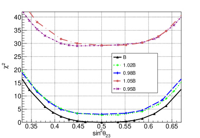
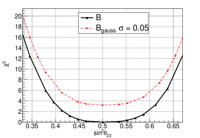
Figure 6: Left: $\Delta\chi^{2}$ as a function of the theory value of $\sin^{2}\theta_{23}$ when the true or data value is fixed to $\sin^{2}\theta_{23}=0.5$; $\Delta m^{2}$ has been marginalised over its $3\sigma$ range. The different curves correspond to theory events generated with a systematically modified magnetic field map, modified by a factor $f$, where $f=1\pm 2\%,1\pm 5$%. It can be seen that 5% field distortion drastically worsens the $\chi^{2}$ and hence the quality of the fit. Right: The same plot for a gaussian variation of the magnetic field map with width $\sigma=0.05$. In both plots the result with true magnetic field map is shown as the solid black line. Note that the $y$ axis ranges are different for the two plots.

6.2 Effect on sensitivity for $\Delta m^{2}$

A similar study was carried out to determine the impact on the sensitivity to the mass squared difference, $\Delta m^{2}$. Here the $\chi^{2}$ was marginalised over the $3\sigma$ range of $\sin^{2}\theta_{23}$ for various theory values of $\Delta m^{2}$.

Systematic change in $B$ field

: From the left hand figure of Fig. 7, again, it can be seen that $\pm 2$% systematic changes in the field map did not cause large changes in the sensitivity. Again, a $\pm 5$% variation is beyond the tolerance limit as the quality of fit worsens considerably. It is interesting to note that unlike in the case of $\sin^{2}\theta_{23}$, the deviation of the best-fit value from the true value is very visible even for small deviations from the true field map. However, we will see below that this is the case for $\sin^{2}\theta_{23}$ as well, although not as clearly visible in Fig. 6.

Gaussian variation in $B$ field

: The sensitivity does not change significantly for a 5% Gaussian variation of the field about its true value, as can be seen from the right panel of Fig. 7. Again, therefore, such fluctuations are more tolerable for precision measurements of $\Delta m^{2}$ than calibration errors in the magnetic field.

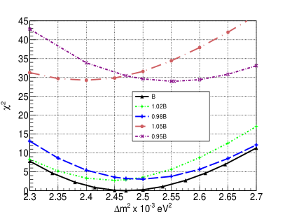
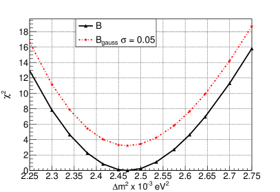
Figure 7: Left: $\Delta\chi^{2}$ as a function of the theory value of $\Delta m^{2}$ in units of eV² when the true or data value is fixed to $\Delta m^{2}=2.47\times 10^{-3}$ eV²; $\sin^{2}\theta_{23}$ has been marginalised over its $3\sigma$ range. The different curves correspond to theory events generated with a systematically modified magnetic field map, modified by a factor $f$, where $f=1\pm 2\%,1\pm 5$%. It can be seen that 5% field distortion drastically worsens the $\chi^{2}$ and hence the quality of the fit. Right: The same plot for a gaussian variation of the magnetic field map with width $\sigma=0.05$. In both plots the result with true magnetic field map is shown as the solid black line. Note that the $y$ axis ranges are different for the two plots.

6.3 Combined fit to $\sin^{2}\theta_{23}$ and $\Delta m^{2}$

In order to better understand the variation of the best fit values with changing magnetic field maps, we have performed a simultaneous 2-parameter fit for each case. The results are shown in Fig. 8 for cases when there is a systematic change in the magnetic field by a factor $|1-f|=2,5$%, as well as for the gaussian case. Shown in blue is the 90% CL contour in the $\sin^{2}\theta_{23}$–$\Delta m^{2}$ plane for the case when the true field map is used to generate both the data and theory. This is the ideal case that has been discussed earlier [20]. The green crosses from top left to bottom right mark the best fit values for $f=0.95$–1.05 in steps of 1% respectively. The dense red square in the centre, at the position of the true (data) values, corresponds to all the cases where the magnetic field map is generated by a gaussian fluctuation of the field around the central value, with width $\sigma=1$–5% in steps of 1%.

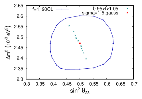
Figure 8: Allowed 90% CL two parameter contour in the $\sin^{2}\theta_{23}$–$\Delta m^{2}$ plane when the true or data value is fixed to $(\sin^{2}\theta_{23},\Delta m^{2})=(0.5,2.47\times 10^{-3}$ eV²) when the true magnetic field map is used to generate the theory events. The green crosses from top left to bottom right correspond to the best-fit values when the magnetic field map used in the theory reconstruction is systematically different from that for the data by $f=0.95$–1.05 in steps of 1% while the red square corresponds to the best-fit values when a gaussian variation upto 5% is used instead. See text for details.

It can be seen that the gaussian fluctuation does not change the best-fit value while systematic errors in the magnetic field map also change both the $\sin^{2}\theta_{23}$ and $\Delta m^{2}$ values systematically away from the true or input data values. The reason for the trend in the best fit values for the case when there is a systematic variation in the field is a consequence of the complicated dependence of the oscillation probabilities on the two parameters of interest. It directly arises from the fact that the reconstructed muon momentum is systematically smaller/larger than the true value when the modified field is systematically smaller/larger than the true map. Since the flux falls severely with neutrino energy, the fact that the cross section increases with energy is unable to compensate for this loss; hence the muon events are peaked at low energies. When this data is fitted using a larger/smaller field map, the peak in the events is shifted to higher/smaller muon energies. The oscillation parameters required to fit this distorted events distribution therefore change. The result has a complicated dependence on the energy as well as direction due to matter effects; see [23] for the dependence of both $P_{\mu\mu}$ and $P_{e\mu}$ on the oscillation parameters as a function of energy and direction of the incoming neutrino. The result however is a straightforward trend in the best fit values as seen in the figure.

Although the best-fit values correspond to increasingly poor $\chi^{2}$ values as the deviation from the true value increases it can be seen from Fig. 8 that variations up to $\pm 5$% yield best-fit values that still lie within the 90% CL of the true result. The minimum $\chi^{2}$ values are shown as a function of the deviations from the true map in Fig. 9. It can be seen that the quality of fit remains decent for gaussian fluctuations of the field around the true value.

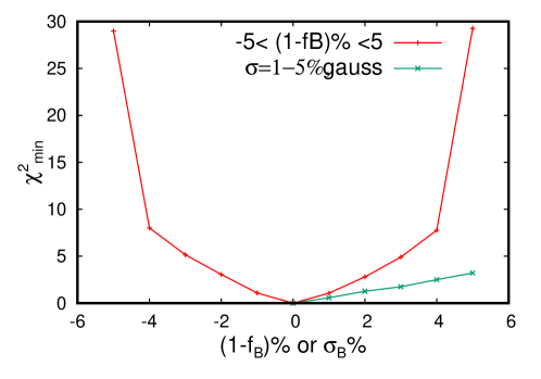
Figure 9: The minimum $\chi^{2}$ value corresponding to the best-fit values shown in Fig. 8 for the simultaneous fit in the $\sin^{2}\theta_{23}$–$\Delta m^{2}$ plane. The red curve with dot points corresponds to the values when the magnetic field map used in the theory reconstruction is systematically different by $\pm 5$% in steps of 1% while the green crosses correspond to the best-fit values when a gaussian variation upto 5% is used instead. See text for details.

6.4 Mass hierarchy sensitivity

Here events were generated using normal ordering (NO) and $\Delta\chi^{2}$ was calculated by assuming the inverted ordering (IO) in the theory. The results were marginalised over $3\sigma$ ranges of both $\sin^{2}\theta_{23}$ and the magnitude of $\Delta m^{2}$. As expected, the sensitivity of the ICAL to the mass ordering decreases with smearing in the $B$-field. However, as can be seen from Fig. 10, the loss of sensitivity is marginal for a $\pm 2$% systematic variation or a 5% gaussian variation of the field, with a $3\sigma$ hierarchy sensitivity being achievable in $11+$ years of running of ICAL rather than $10+$ years with ideal field map.

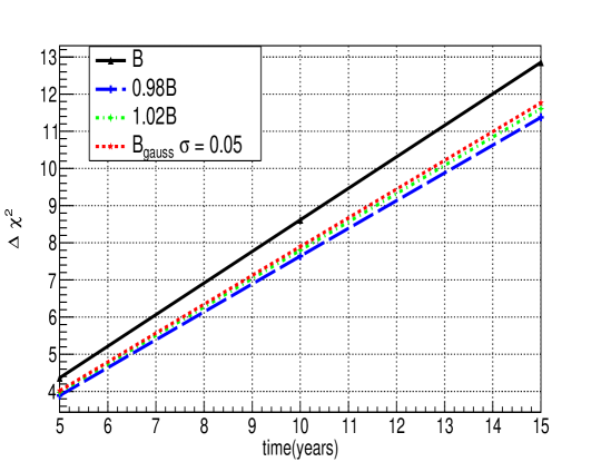
Figure 10: Ability to discriminate against the wrong mass ordering as a function of exposure time in years at ICAL with theory events being generated according to true map (black solid line), showing a loss in sensitivity when there is a $\pm 2$% systematic deviation in the map (green and blue dashed and dotted lines), and a marginal improvement (red dotted line) when a 5% gaussian modified map is used.

7 Discussion and conclusions

We have presented, for the first time, a detailed simulations analysis of the realistic case when the magnetic field map for ICAL is not precisely known, and the consequent impact on the precision with which the oscillation parameters, especially in the 2–3 sector can be determined in this case. We have used the magnetic field measurements made on the prototype mini-ICAL 85 ton detector which is an exact scale model of the proposed ICAL detector to determine reasonable ranges of errors, both in measurement and calibration, of the magnetic field. First, we generated 250 sets of 10,000 muon events each at different energies and angles in a Geant4 simulation of the ICAL detector. The resulting muon tracks were then reconstructed and analysed using (1) the true map, (2) maps that deviated from the true map systematically by a constant factor $f$, being either larger than or smaller than the true field. It was found that for small deviations of the map, the deviations in the reconstructed muon momentum showed a linear dependence on the deviation of the magnetic field, and was non-linear for larger deviations. It was further found that these variations were independent of the region in ICAL where the event was generated. The muon momentum resolution also changed linearly, although the variation of this parameter does not significantly affect the results. It was also found that, within reasonable errors, the reconstruction efficiency, charge-id efficiency, and the angular resolution remained the same as with the true magnetic field map.

This study was then used to parametrise the muon parameters (energy, resolution functions, etc) in terms of the magnetic field parameter $f$. This enabled analysis for arbitrary values of the magnetic field. In addition, five systematic errors corresponding to pulls for flux and cross section normalisation, flux angular distribution, flux energy dependence or tilt, and detector parameters, were included in the analysis. It was found that small systematic deviations from the true field gave acceptable results with very little loss of sensitivity to the 2–3 oscillation parameters $\sin^{2}\theta_{23}$ and $\Delta m^{2}$ (or equivalently, $\Delta m^{2}_{32}$). However, large variations of say 5%led to very bad quality fits. It appears that poor quality fits may be useful as an indicator of issues with calibration of the magnetic field and is an important outcome of this study for the main ICAL detector.

Random fluctuations of the magnetic field in different regions of ICAL with gaussian widths of 5% around the true magnetic field value, on the other hand, gave results with very good quality fits for both the 2–3 parameters; in addition the resulting best-fit parameters were very close to the true input values, in contrast to the case when there are systematic variations in the magnetic field. Hence, errors, especially in the calibration of the magnetic field map, may give rise to best-fit values which trend away from the true values, depending on the size of the deviations.

As mentioned earlier, this is the first detailed study of the impact of errors in the measurement of the magnetic field in ICAL on the quality and correctness of the fits to the neutrino oscillation parameters $\sin^{2}\theta_{23}$ and $\Delta m^{2}_{32}$. More data is being currently taken at the prototype mini-ICAL detector in Madurai, South India. In addition, detailed simulations studies of the magnetic field map for both the main ICAL and mini-ICAL are on-going and will be compared to the measured values. Both these will augment this current first and preliminary analysis and allow for a more detailed study of this crucial input to ICAL physics.

Acknowledgements

: We thank V.M. Datar and Amol Dighe for a careful reading of the manuscript and many clarifications, and the members of the ICAL collaboration for support and discussions.

References

- [1] Ahmed, Shakeel et al., ICAL collab., Physics Potential of the ICAL detector at the India-based Neutrino Observatory (INO), Pramana 88 (2017) 79, arXiv:1505.07380 [physics.ins-det], doi 10.1007/s12043-017-1373-4.
- [2] Davis, R., A review of the Homestake solar neutrino experiment, Prog. Part. Nucl. Phys. 32 (1994), 13–32, doi 10.1016/0146-6410(94)90004-3.
- [3] Chatterjee, A., Meghna, K. K., Rawat, Kanishka, Thakore, T., Bhatnagar, V., Gandhi, R., Indumathi, D., Mondal, N. K., and Sinha, Nita, A Simulations Study of the Muon Response of the Iron Calorimeter Detector at the India-based Neutrino Observatory, JINST 9, P07001 (2014), arXiv:1405.7243, physics.ins-det, doi 10.1088/1748-0221/9/07/P07001.
- [4] Pontecorvo, Bruno, Neutrino experiments and the problem of conservation of leptonic charge, Sov. Phys. JETP 26 (1968) 165.
- [5] Maki, Ziro, Nakagawa, Masami and Sakata, Shoichi, Remarks on the Unified Model of Elementary Particles, Progress of Theoretical Physics 28 (1962), 870-880, doi 10.1143/PTP.28.870.
- [6] Abi, B. et al., DUNE collab., Long-baseline neutrino oscillation physics potential of the DUNE experiment, Eur. Phys. J. C 80 (2020) 978, doi 10.1140/epjc/s10052-020-08456-z, arXiv:2006.16043 [hep-ex].
- [7] Abusleme, Angel et al., JUNO collab., Sub-percent precision measurement of neutrino oscillation parameters with JUNO, Chin. Phys. C 46 (2022), 123001, doi 10.1088/1674-1137/ac8bc9, arXiv:2204.13249 [hep-ex].
- [8] P. A. Zyla et al. [Particle Data Group], PTEP 2020, no.8, 083C01 (2020) doi:10.1093/ptep/ptaa104
- [9] I. Esteban, M. C. Gonzalez-Garcia, M. Maltoni, T. Schwetz and A. Zhou, JHEP 09, 178 (2020) doi:10.1007/JHEP09(2020)178 [arXiv:2007.14792 [hep-ph]].
- [10] Senthil, R. Thiru, Indumathi, D. and Shukla, Prashant, Simulation study of tau neutrino events at the ICAL detector in INO, Phys. Rev. D 106 (2022) 093004, arXiv:2203.09863 [hep-ph], doi 10.1103/PhysRevD.106.093004.
- [11] Wolfenstein, L., Neutrino Oscillations in Matter, Phys. Rev. D 17 (1978) 2369–2374, doi 10.1103/PhysRevD.17.2369.
- [12] Mikheev, S. P. and Smirnov, A. Yu., Resonant amplification of neutrino oscillations in matter and solar neutrino spectroscopy, Nuovo Cim. C 9 (1986) 17–26, doi 10.1007/BF02508049.
- [13] Behera, Shiba P., Bhatia, Manmohan S., Datar, Vivek M. and Mohanty, Ajit K., Simulation Studies for Electromagnetic Design of INO ICAL Magnet and Its Response to Muons, IEEE Transactions on Magnetics 51 (2015) 1-9, doi=10.1109/TMAG.2014.2344624.
- [14] Infolytica Corp., Electromagnetic field simulation software, http://www.infolytica.com/en/products/magnet/.
- [15] Khindri Honey et al., Magnetic field measurements on the mini-ICAL detector using Hall probes, JINST 17 (2022) T10006, arXiv: 2206.15082 [physics.ins-det], doi 10.1088/1748-0221/17/10/T10006.
- [16] H. Khindri et al., Simulations studies of the magnetic field in the mini-ICAL prototype using MAGNET software, 2023, in preparation.
- [17] S. Agostinelli et al., Geant4, a simulation toolkit, Nucl. Instr. Meth. in Physics Res. A 506 (2003), 250.
- [18] Kanishka, R., Meghna, K. K., Bhatnagar, V., Indumathi, D. and Sinha, N., Simulations Study of Muon Response in the Peripheral Regions of the Iron Calorimeter Detector at the India-based Neutrino Observatory, JINST 10 (2015) P03011, arXiv:1503.03369 [physics.ins-det], doi 10.1088/1748-0221/10/03/P03011.
- [19] Devi, M. M., Dighe, A., Indumathi, D. and Lakshmi, S. M., Simulation studies of reconstruction of hadron shower direction in INO ICAL detector, JINST 13 (2018) C03006, doi = ”10.1088/1748-0221/13/03/C03006”,
- [20] Lakshmi S. Mohan and D. Indumathi, Pinning down neutrino oscillation parameters in the 2–3 sector with a magnetised atmospheric neutrino detector: a new study, The European Physical Journal C 77 (2017) 54, arXiv:1605.04185 [hep-ph], doi 10.1140/epjc/s10052-017-4608-0.
- [21] Casper, D., The Nuance neutrino physics simulation, and the future, Nucl. Phys. B Proc. Suppl. 112 (2002) 161–170, arXiv:hep-ph/0208030, doi 10.1016/S0920-5632(02)01756-5.
- [22] Honda, Morihiro, Kajita, T., Kasahara, K. and Midorikawa, S., A New calculation of the atmospheric neutrino flux in a 3-dimensional scheme, Phys. Rev. D 70 (2004) 043008, arXiv: astro-ph/0404457, doi 10.1103/PhysRevD.70.043008.
- [23] Indumathi, D., Murthy, M.V.N., Rajasekaran, G. and Sinha, Nita, Neutrino oscillation probabilities: Sensitivity to parameters, Phys. Rev. bf D 74 (2006) 053004, arXiv:hep-ph/0603264, doi 10.1103/PhysRevD.74.053004.