RepCL: Exploring Effective Representation for Continual Text Classification

Abstract

Continual learning (CL) aims to constantly learn new knowledge over time while avoiding catastrophic forgetting on old tasks. In this work, we focus on continual text classification under the class-incremental setting. Recent CL studies find that the representations learned in one task may not be effective for other tasks, namely representation bias problem. For the first time we formally analyze representation bias from an information bottleneck perspective and suggest that exploiting representations with more class-relevant information could alleviate the bias. To this end, we propose a novel replay-based continual text classification method, RepCL. Our approach utilizes contrastive and generative representation learning objectives to capture more class-relevant features. In addition, RepCL introduces an adversarial replay strategy to alleviate the overfitting problem of replay. Experiments demonstrate that RepCL effectively alleviates forgetting and achieves state-of-the-art performance on three text classification tasks.

1 Introduction

Continual learning (CL) enables conventional static natural language processing models to constantly gain new knowledge from a stream of incoming data (Sun et al., 2020; Biesialska et al., 2020). In this paper, we focus on continual text classification, which is formulated as a class-incremental problem, requiring the model to learn from a sequence of class-incremental tasks (Huang et al., 2021). Figure 1 gives an illustrative example of continual text classification. The model needs to learn to distinguish some new classes in each task and is eventually evaluated on all seen classes. Like other CL systems, the major challenge of continual text classification is catastrophic forgetting (Lange et al., 2022): after new tasks are learned, performance on old tasks may degrade dramatically.

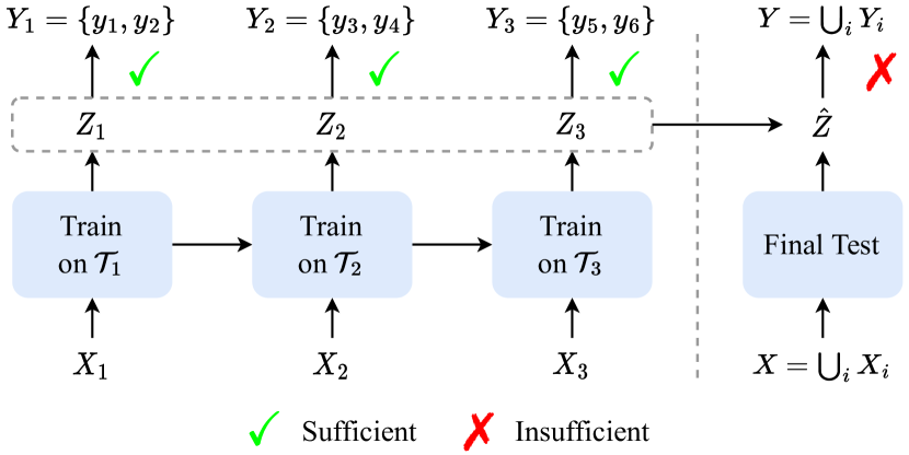
Figure 1: Illustration for continual text classification with three tasks where each task involves two new classes. $X_{i}$, $Y_{i}$, and $Z_{i}$ denote input sentences, new classes and learned representations for $i$-th task $\mathcal{T}_{i}$ respectively. Although the representations $Z_{i}$ learned in $\mathcal{T}_{i}$ are sufficient for classifying $Y_{i}$, they are ineffective to distinguish all seen classes $Y$ in the final test.

The earlier work in the CL community mainly attributes catastrophic forgetting to the corruption of the learned representations as new tasks arrive and various methods have been introduced to retain or recover previously learned representations (Kirkpatrick et al., 2017; Rebuffi et al., 2017; Mallya and Lazebnik, 2018; Lange et al., 2022). Recently, some studies find that, under the sequential task setting, CL models tend to only capture useful features for the current task and cannot learn effective representations with consideration of the entire CL process, which is named as representation bias and maybe the main reason for catastrophic forgetting (Cha et al., 2021; Guo et al., 2022; Wang et al., 2022b). To alleviate representation bias, Guo et al. (2022) propose the InfoMax model to greedily preserve the input features as much as possible and Wang et al. (2022b) exploit an adversarial class augmentation mechanism. However, both InfoMax and heuristic augmentation will introduce excessive noise into representations which may harm the generalization (Tian et al., 2020).

To explore reasonable and effective representations, in this paper, for the first time we formally analyze the representation bias problem from the information bottleneck (IB) (Tishby et al., 2000; Tishby and Zaslavsky, 2015) perspective. Specifically, we formulate the learning process of CL as a trade-off between representation compression and preservation, and empirically measure the mutual information of the learned representations. Then we derive the following conclusions that, (1) in each individual task, due to the compression effect of IB, CL models discard features irrelevant to current task and cannot learn sufficient representations for cross-task classes; (2) effective representations for CL should “globally” balance feature preservation and task-irrelevant information compression for the entire continual task. Since it is impossible to foresee future classes and identify crucial features for future tasks, we suppose that the key problem is how to design representation learning objectives for capturing more class-relevant features.

Based on our analysis, we propose a replay-based continual text classification method RepCL. RepCL utilizes both contrastive and generative representation learning objectives to learn class-relevant features from each individual task. The contrastive objective explicitly maximizes the mutual information between representations of instances from the same class. The generative objective instructs the representation learning process through reconstructing corrupted sentences from the same class, which implicitly makes the model capture more class-relevant features. In addition, to better protect the learned representations, RepCL also incorporates an adversarial replay mechanism to alleviate the overfitting problem of the replay.

Our contributions are summarized as follows: (i) We formally analyze representation bias in CL from an information bottleneck perspective and suggest that learning more class-relevant features will alleviate the bias. (ii) We propose a novel continual text classification method RepCL, which exploits contrastive and generative representation learning objectives to handle the representation bias. (iii) Experimental results on three text classification tasks show that RepCL learns more effective representations and significantly outperforms state-of-the-art methods.

2 Related Work

Continual Learning

Continual Learning (CL) studies the problem of continually learning knowledge from a sequence of tasks without the need to retrain from scratch Lange et al. (2022). The major challenge of CL is catastrophic forgetting. Previous CL works mainly attribute catastrophic forgetting to the corruption of learned knowledge. To this end, three major families of approaches have been developed. Replay-based methods (Rebuffi et al., 2017; Prabhu et al., 2020) save a few previous task instances in a memory module and retrain on them while training of new tasks. Regularization-based methods (Kirkpatrick et al., 2017; Aljundi et al., 2018) introduce an extra regularization term in the loss function to consolidate previous knowledge. Parameter-isolation methods (Mallya and Lazebnik, 2018) dynamically expand the network and dedicate different model parameters to each task. Despite the simplicity, replay-based methods have been proven to be effective (Buzzega et al., 2020; Wang et al., 2019). However, replay-based methods suffer from overfitting the few stored data. In this paper, we introduce an adversarial replay strategy to alleviate the overfitting problem of replay.

Representation Learning in CL

Most previous work in CL focuses on retaining or recovering learned representations, whereas a few recent studies find that CL models suffer from representation bias: CL models tend to only capture useful features for the current task and cannot learn effective representations with consideration of the entire CL process (Guo et al., 2022; Wang et al., 2022b). To mitigate the bias, Wang et al. (2022b) design two adversarial class augmentation strategies for continual relation extraction. Guo et al. (2022) introduce a mutual information maximization method to preserve the features as much as possible for online continual image classification. However, both heuristic data augmentation and InfoMax method may introduce task-irrelevant noise, which could lead to worse generalization on the task (Tian et al., 2020). Unlike previous work, in this paper, we formally analyze representation bias from the information bottleneck perspective and propose a more reasonable training objective that makes a trade-off between representation compression and preservation ability.

3 Task Formulation

In this work, we focus on continual learning for a sequence of $k$ class-incremental text classification tasks $(\mathcal{T}_{1},\mathcal{T}_{2},...,\mathcal{T}_{k})$. Each task $\mathcal{T}_{i}$ has its dataset $\mathcal{D}_{i}=\{(x_{i}^{(j)},y_{i}^{(j)})\}$, where $(x_{i}^{(j)},y_{i}^{(j)})$ is an instance of current task and is sampled from an individually i.i.d. distribution $p(X_{i},Y_{i})$. Different tasks $\mathcal{T}_{i}$ and $\mathcal{T}_{j}$ have disjoint label sets $Y_{i}$ and $Y_{j}$. The goal of CL is to continually train the model on new tasks to learn new classes while avoiding forgetting previously learned ones. From another perspective, if we denote $X=\cup_{i}X_{i}$ and $Y=\cup_{i}Y_{i}$ as the input and output space of the entire CL process respectively, continual learning is aiming to approximate a holistic distribution $p(Y|X)$ from a non-i.i.d data stream.

The text classification model $F$ is usually composed of two modules: the encoder $f$ and the classifier $\sigma$. For an input $x$, we get the corresponding representation $z=f(x)$, and use the logits $\sigma\left(z\right)$ to compute loss and predict the label.

4 Representation Bias in CL

Previous work (Cha et al., 2021; Guo et al., 2022; Wang et al., 2022b; Xia et al., 2023) reveals that representation bias is an important reason for catastrophic forgetting. In this section, we analyze the representation bias problem from an information bottleneck (IB) perspective and further discuss what representations are effective for CL.

4.1 Information Bottleneck

We first briefly introduce the background of information bottleneck in this section. Information bottleneck formulates the goal of deep learning as an information-theoretic trade-off between representation compression and preservation (Tishby and Zaslavsky, 2015; Shwartz-Ziv and Tishby, 2017). Given the input $\mathcal{X}$ and the label set $\mathcal{Y}$, one model is built to learn the representation $\mathcal{Z}=\mathcal{F}(\mathcal{X})$ of the encoder $\mathcal{F}$. The learning procedure of the model is to minimize the following Lagrangian:

$$I(\mathcal{X};\mathcal{Z})-\beta I(\mathcal{Z};\mathcal{Y}),$$ (1)

where $I(\mathcal{X};\mathcal{Z})$ is the mutual information (MI) between $\mathcal{X}$ and $\mathcal{Z}$, and $\beta$ is a trade-off hyperparameter. With information bottleneck, the model will learn minimal sufficient representation $\mathcal{Z}^{*}$ (Achille and Soatto, 2018) of $\mathcal{X}$ corresponding to $\mathcal{Y}$:

$$\mathcal{Z}^{*}=\arg\min_{\mathcal{Z}}I(\mathcal{X};\mathcal{Z})$$ (2)

$$\mathrm{s.t.}\ I(\mathcal{Z};\mathcal{Y})=I(\mathcal{X};\mathcal{Y}).$$ (3)

Minimal sufficient representation is important for supervised learning, because it retains as little about input as possible to simplify the role of the classifier and improve generalization, without losing information about labels.

4.2 Representation Bias: the IB Perspective

In this section, we investigate representation bias from the IB perspective. Continual learning is formulated as a sequence of individual tasks $(\mathcal{T}_{1},\mathcal{T}_{2},...,\mathcal{T}_{k})$. For $i$-th task $\mathcal{T}_{i}$, the model aims to approximate distribution $p(Y_{i}|X_{i})$. According to IB, if the model $F=\sigma\circ f$ converges, the learned hidden representation $Z_{i}=f(X_{i})$ will be minimal sufficient for $\mathcal{T}_{i}$:

$$Z_{i}=\arg\min_{Z_{i}}I\left(X_{i};Z_{i}\right)$$ (4)

$$\mathrm{s.t.}\ I\left(Z_{i};Y_{i}\right)=I(X_{i};Y_{i}),$$ (5)

which ensures the performance and generalization ability of the current task. Nevertheless, the minimization of the compression term will bring potential risks: features that are useless in the current task but crucial for other tasks will be discarded.

For the entire continual learning task with the holistic target distribution $p(Y|X)$, the necessary condition to perform well is that the representation $Z$ is sufficient for $Y$: $I(Z;Y)=I(X;Y)$. However, as some crucial features are compressed, the combination of minimal sufficient representations for each task $Z=\cup_{i}Z_{i}$ may be insufficient:

$$I\left(Z;Y\right)<I(X;Y).$$ (6)

Therefore, from the IB perspective, representation bias can be reformulated as: due to the compression effect of IB, the learned representations in each individual task may be insufficient for the entire continual task.

Models	FewRel		MAVEN
	$I(X_{1};Z_{1})$	$I(Z;Y)$	$I(X_{1};Z_{1})$	$I(Z;Y)$
Supervised	2.42	2.45	3.50	2.42
CRL	2.12	2.18	3.12	2.30
CRECL	2.20	2.31	3.01	2.36
FEA	2.35	2.34	3.17	2.37

Table 1: Mutual information comparison between supervised learning and strong CL baselines on FewRel and MAVEN datasets. We use $I(X;Z)$ to measure how much features of input $X$ representation $Z$ preserves. To exclude the impact of representation corruption, we instead estimate $I(X_{1};Z_{1})$ after CL models finish $\mathcal{T}_{1}$. $I(Z;Y)$ measures whether the learned representation is sufficient for the entire continual task.

To confirm our analysis, we use supervised learning on all data as the baseline, and compare MI between supervised learning with several strong CL baselines. Concretely, we use MINE (Belghazi et al., 2018) as the MI estimator and conduct experiments on FewRel and MAVEN dataset. First, we measure $I(X;Z)$ to estimate the amount of features preserved by the representation $Z$. However, previously learned representations will be corrupted after the model learns new tasks, which will make our estimation inaccurate. To exclude the impact of representation corruption, we instead estimate $I(X_{1};Z_{1})$ on $\mathcal{T}_{1}$’s test set. Second, to measure whether learned representations are sufficient for the entire continual task, we compare $I(Z;Y)$ on the final test set with all classes. As shown in Table 1, both $I(X_{1};Z_{1})$ and $I(Z;Y)$ of three CL models are significantly lower than supervised learning, indicating that the CL model tends to compress more information due to the individual task setting and the representations learned in CL are insufficient for the entire continual task.

4.3 What are Effective CL Representations?

Since minimization of the compression term $I(\mathcal{X};\mathcal{Z})$ in IB leads to representation bias in CL, the most straightforward solution is to defy it when learning new tasks. Specifically, in $i$-th task $\mathcal{T}_{i}$, we can maximize $I\left(X_{i};Z_{i}\right)$ and force the representation to retain information about input as much as possible (Guo et al., 2022) (we will omit subscripts $i$ for brevity of notation). However, Tian et al. (2020) find that the InfoMax principle may introduce task-irrelevant noisy information, which could lead to worse generalization.

Ideally, the effective representation learning objective of CL should be a “global” IB trade-off between feature preservation and task-irrelevant information compression for the entire continual task. Due to the sequential task setting of CL, we cannot foresee future tasks and identify crucial features for the entire continual task in advance. Nevertheless, if we can capture the “essence” features closely relevant to a specific class, then the representation is discriminative with any other classes. On the other hand, without knowing future tasks, any information shared by instances of the same class are potentially useful for the entire CL process. Therefore, we propose that a more effective representation learning objective for new tasks is to learn more class-relevant features, which can improve the sufficiency of the representations with as little impact on the generalization of the current task as possible. The empirical results in Section 7.2 also show that learning more class-relevant features has better performance than directly maximizing $I(X;Z)$.

5 Methodology

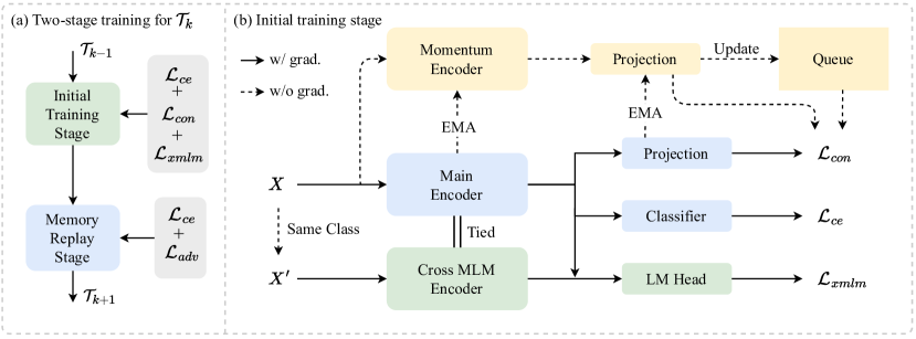
Figure 2: (a) A demonstration for RepCL, which is based on the two-stage training backbone. (b) Framework of initial training stage of InfoCL, which can be decomposed into (yellow) momentum branch, (blue) main branch, (green) XMLM branch. In the memory replay stage and at inference time, we discard momentum branch and XMLM branch, only preserving the main branch.

Based on our analysis, we propose a novel replay-based continual learning method, RepCL, which helps the model learn more class-relevant features to better alleviate representation bias.

Following recent work (Mai et al., 2022; Wang et al., 2022b), we adapt our method to the two-stage training backbone, which can effectively alleviate the classifier bias problem for replay-based methods. Concretely, the training process on a task is divided into the initial training and memory replay stages. In the initial training stage, the model is trained with only current task data to learn the new task. In the memory replay stage, we first select a few typical instances from new task data to update memory and then train the model with the balanced memory bank to recover previously learned knowledge.

The overall structure of RepCL is illustrated in Figure 2. In Section 5.1 and 5.2, we introduce contrastive and generative representation learning for the initial training stage to learn class-relevant representations and mitigate representation bias. In Section 5.3, we propose an adversarial replay mechanism in the memory replay stage to better recover corrupted old representations.

5.1 Contrastive Representation Learning

If we denote $Z$ and $Z^{+}$ as the representations corresponding to instances $X$ and $X^{+}$ with the same label, $I(Z;Z^{+})$ measures the amount of class-relevant features contained in representations. Due to the intractability of computing MI, we instead use contrastive loss SupInfoNCE (Barbano et al., 2022) as a proxy to maximize a lower bound on $I\left(f(X);f(X^{+})\right)$ to learn more class-relevant features:

where $g(x_{1},x_{2})=f(x_{1})\cdot f(x_{2})/\tau$ computes the representation similarity of two instances, $x^{+}$ is the positive instance with the same label as $x$, $x^{-}$ is an instance of the current batch $\mathcal{B}$, and $\tau$ is the temperature hyperparameter.

As the number of negative instances increases, SupInfoNCE will be a tighter bound of MI (van den Oord et al., 2018; Poole et al., 2019). Therefore, to effectively enlarge the number of negative instances, following MoCoSE (Cao et al., 2022), we build a contrastive learning model consisting of a two-branch structure and a queue. The upper two branches of Figure 2(b) depicts the architecture. As illustrated, we add a projection layer on both of the main branch and the momentum branch. For the queue, same as He et al. (2020); Cao et al. (2022), it is updated with the output of momentum branch by first-in-first-out strategy.

As mentioned before, we use SupInfoNCE as contrastive representation learning objective:

where $z$ is the anchor vector obtained by the main branch, $z_{i}^{+}$ refers to the vector obtained by the momentum branch or stored in the queue which has the same class label as the anchor, and $z^{-}$ are the negative instances in the momentum branch or in the queue which belong to different classes with anchor, $\tau$ is the temperature hyperparameter.

The model calculates $\mathcal{L}_{\mathrm{con}}$ and backwards to update the main branch. The momentum branch truncates the gradient and is updated with exponential moving average (EMA) method during training. Formally, denoting the parameters of the main and momentum branches as $\theta$ and $\theta^{\prime}$, $\theta^{\prime}$ is updated by:

$$\theta^{\prime}\leftarrow\eta\theta^{\prime}+(1-\eta)\theta,$$ (9)

where $\eta$ is the EMA decay rate.

5.2 Generative Representation Learning

In Eq. 8, to make SupInfoNCE an unbiased MI estimator, the negative instances $z^{-}$ should be sampled from the whole input space. However, in CL scenario, $z^{-}$ are still sampled from the current task, thus the effectiveness of contrastive learning may be limited. Inspired by recent generative sentence representation work (Yang et al., 2021; Wu and Zhao, 2022), we additionally introduce a novel cross masked language modeling (XMLM) training objective to encourage the learned representations to contain more class-relevant information.

The lower two branches in Figure 2(b) illustrate the architecture of XMLM. For instance $x$, we randomly sample another instance $x^{\prime}$ with the same class label as $x$ from the current task’s training set. Then $x^{\prime}$ is masked in a certain proportion, and fed into the XMLM encoder, which shares the same weights with the main branch encoder. The masked language modeling task of $x^{\prime}$ is aided by representation $f(x)$ output by the main encoder. Specifically, we concatenate $f(x)$ with the hidden states of token [MASK] in $x^{\prime}$ to predict the corresponding masked token and compute MLM loss $\mathcal{L}_{\mathrm{xmlm}}$. Intuitively, if the representation $f(x)$ contains more class-relevant information, it will be helpful for the XMLM branch to recover the corrupted sentence from the same class. We empirically compare XMLM with vanilla MLM in Section 7.1.

When a new task comes, we first initialize a new momentum branch and XMLM branch. Then in the initial training stage we optimize the model with the combination of cross-entropy loss, contrastive loss, and XMLM loss as objective:

$$\mathcal{L}_{\mathrm{init}}=\mathcal{L}_{\mathrm{ce}}+\lambda_{1}\mathcal{L}_{\mathrm{con}}+\lambda_{2}\mathcal{L}_{\mathrm{xmlm}},$$ (10)

where $\lambda_{1},\lambda_{2}$ are weighting coefficients. In the memory replay stage and at inference time, we discard the momentum branch and XMLM branch, only using the output of the main branch classifier to predict the label of an instance.

5.3 Adversarial Replay

After the initial training stage, we first select and store typical instances for each class for replay. Following Cui et al. (2021) and Zhao et al. (2022), for each class, we use K-means to cluster the corresponding representations, and the instances closest to the centroids are stored in the memory bank.

Then we use the instances of all seen classes in the memory bank to conduct the memory replay stage. The replay strategy is widely used to recover corrupted representations, whereas its performance is always hindered by the overfitting problem due to the limited memory budget. To alleviate overfitting and enhance the effect of recovering, we incorporate FreeLB (Zhu et al., 2020) adversarial loss into the supervised training objective:

Please refer to Appendix B for details about Eq. 11. Intuitively, FreeLB performs multiple adversarial attack iterations to craft adversarial examples, which is equivalent to replacing the original batch with a $K$-times larger adversarial augmented batch.

The optimization objective in the memory replay stage is the combination of $\mathcal{L}_{\mathrm{adv}}$ and conventional cross entropy loss $\mathcal{L}_{\mathrm{ce}}$:

$$\mathcal{L}_{\mathrm{replay}}=\mathcal{L}_{\mathrm{ce}}+\mathcal{L}_{\mathrm{adv}}.$$ (12)

Datasets	FewRel		TACRED		MAVEN		HWU64
Models	Acc $\uparrow$	FR $\downarrow$	Acc $\uparrow$	FR $\downarrow$	Acc $\uparrow$	FR $\downarrow$	Acc $\uparrow$	FR $\downarrow$
IDBR (Huang et al., 2021)	68.9	30.4	60.1	35.3	57.3	34.2	76.1	19.0
KCN (Cao et al., 2020)	76.0	23.2	70.6	22.3	64.4	29.0	81.9	13.5
KDRK (Yu et al., 2021)	78.0	18.4	70.8	22.8	65.4	28.3	81.4	14.0
EMAR (Han et al., 2020)	83.6	12.1	76.1	20.0	73.2	14.6	83.1	9.3
RP-CRE (Cui et al., 2021)	82.8	10.3	75.3	17.5	74.8	11.4	82.7	10.9
CRL (Zhao et al., 2022)	83.1	11.5	78.0	18.0	73.7	11.2	81.5	9.9
CRECL (Hu et al., 2022)	82.7	11.6	78.5	16.3	73.5	13.8	81.1	9.8
FEA (Wang et al., 2022a)	84.3	8.9	77.7	13.3	75.0	12.8	83.3	8.8
ACA (Wang et al., 2022b)	84.7	11.0	78.1	13.8	–	–	–	–
RepCL (Ours)	85.6	8.7	78.6	12.0	75.9	10.7	84.8	8.0

Table 2: Accuracy (Acc) and forgetting rate (FR) on all seen classes after learning the final task. We report the average result of $5$ different runs. The best results are in boldface. ACA is specially designed for continual relation extraction and cannot be adapted to other tasks. CRECL is a concurrent work to ours.

6 Experiments

6.1 Experiment Setups

Datasets

To fully measure the ability of RepCL, we conduct experiments on 4 datasets for 3 different text classification tasks, including relation extraction, event classification, and intent detection. For relation extraction, following previous work (Han et al., 2020; Cui et al., 2021; Zhao et al., 2022), we use FewRel (Han et al., 2018) and TACRED (Zhang et al., 2017). For event classification, following Yu et al. (2021) and Wu et al. (2022), we use MAVEN (Wang et al., 2020) to build our benchmark. For intent detection, following Liu et al. (2021), we choose HWU64 (Liu et al., 2019) dataset. For the task sequence, we simulate 10 tasks by randomly dividing all classes of the dataset into 10 disjoint sets, and the number of new classes in each task for FewRel, TACRED, MAVEN and HWU64 are 8, 4, 12, 5 respectively. For a fair comparison, the result of baselines are reproduced on the same task sequences as our method. Please refer to Appendix C for details of these four datasets.

Evaluation Metrics

Following previous work (Hu et al., 2022; Wang et al., 2022b), we use the average accuracy (Acc) on all seen tasks as our main metric. In addition to, we also use the average forgetting rate (FR) (Chaudhry et al., 2018) to quantify the accuracy drop of old tasks. CL methods with lower forgetting rates have less forgetting on previous tasks. The detailed computation of FR is given in Appendix D.

Baselines

We compare RepCL against the following baselines: IDBR (Huang et al., 2021), KCN (Cao et al., 2020), KDRK (Yu et al., 2021), EMAR (Han et al., 2020), RP-CRE (Cui et al., 2021), CRL (Zhao et al., 2022), CRECL (Hu et al., 2022), FEA (Wang et al., 2022a) and ACA (Wang et al., 2022b). Note that FEA (Wang et al., 2022a) can be seen as the two-stage training backbone of RepCL. See Appendix E for details of our baselines.

Some baselines are originally proposed to tackle one specific task. For example, RP-CRE is designed for continual relation extraction. We adapt these baselines to other tasks and report the corresponding results. Although the continual image classification work Cha et al. (2021) and Guo et al. (2022) are also conceptually related to our work, their methods rely on specific image augmentation mechanisms and cannot be adapted to the continual text classification task.

Implementation Details

For RepCL, we use BERT_base (Devlin et al., 2019) as the encoder following previous work Cui et al. (2021); Wang et al. (2022b). The learning rate of RepCL is set to 1e-5 for the BERT encoder and 1e-3 for other modules. Hyperparameters are tuned on the first three tasks. The memory budget for each class is fixed at 10 for all methods. For all experiments, we use NVIDIA A40 and RTX 3090 GPUs and report the average result of 5 different task sequences. More implementation details can be found in Appendix F.

6.2 Main Results

Table 2 shows the performance of RepCL and baselines on four datasets for three text classification tasks. Due to space constraints, we only illustrate Acc after learning the final task and FR. The complete accuracy of all 10 tasks can be found in Appendix G. As shown, our proposed RepCL consistently outperforms all baselines (except CRECL in TACRED) with significance test $p<0.05$ and achieves new state-of-the-art results on all four benchmarks. Furthermore, compared with baselines on all tasks, RepCL has a substantially lower forgetting rate, which indicates that our method can better alleviate catastrophic forgetting. These experimental results demonstrate the effectiveness and universality of our proposed method.

7 Analysis

7.1 Ablation Study

Models	Few.	TAC.	MAV.	HWU.
RepCL	85.6	78.6	75.9	84.8
w/o $\mathcal{L}_{\mathrm{con}}$	85.3	78.1	75.6	84.5
w/o $\mathcal{L}_{\mathrm{xmlm}}$	84.8	77.9	75.5	84.1
w/o $\mathcal{L}_{\mathrm{adv}}$	85.3	78.0	75.9	83.8
w/ MLM	85.0	78.2	75.3	84.3

Table 3: Ablation study of RepCL. “w/ MLM” denotes replacing cross MLM objective with a conventional masked language modeling objective.

We conduct an ablation study to investigate the effectiveness of different components of RepCL. The results are shown in Table 3. We find that the three core mechanisms of RepCL, namely contrastive and generative objectives for learning new tasks, and adversarial replay for the replay stage, are conducive to the model performance. Note the generative objective $\mathcal{L}_{\mathrm{xmlm}}$ is more effective than the contrastive objective $\mathcal{L}_{\mathrm{con}}$. We attribute this to the fact that negative instances for contrastive learning are not sampled from the whole input space, which has been discussed in Section 5.2.

To better understand our proposed generative objective, we replace XMLM with the conventional MLM objective and conduct experiments. Specifically, in the XMLM branch, we remove the concatenation of the main branch representation. As shown, training with MLM leads to performance degradation, indicating that vanilla MLM cannot effectively guide the representations to contain more class-relevant information.

7.2 Effective Representation Learning

In Section 4.3, we suggest that learning more class-relevant features is a better training objective to alleviate representation bias in CL, which makes a trade-off between crucial feature preservation and noisy information compression. Since FEA (Wang et al., 2022a) can be seen as the backbone of our method, we compare RepCL with FEA and its InfoMax variant FEA+InfoMax, which replaces our proposed contrastive and generative learning objectives with InfoNCE as Gao et al. (2021) to maximize $I(X;Z)$ in the initial training stage. To exclude the impact of representation corruption, we choose $\mathcal{T}_{1}$ and estimate $I(X_{1};Z_{1})$ and $I\left(Z_{1};Z_{1}^{+}\right)$ of representations learned by different methods.

Models	FEA	FEA+InfoMax	RepCL
$I(X_{1};Z_{1})$	2.35	2.44	2.41
$I(Z_{1};Z_{1}^{+})$	1.99	1.99	2.01
Final Acc	84.3	84.7	85.6

Table 4: $I(X_{1};Z_{1})$ and $I(Z_{1};Z_{1}^{+})$ of test set in $\mathcal{T}_{1}$ of FewRel. Since the estimate process of $I(Z_{1};Z_{1}^{+})$ is not stable, we illustrate the estimator fitting curves in Figure 3(a). FEA+InfoMax introduces InfoNCE loss following Gao et al. (2021) to maximise $I(X;Z)$. We also report the final accuracy on all tasks for three methods.

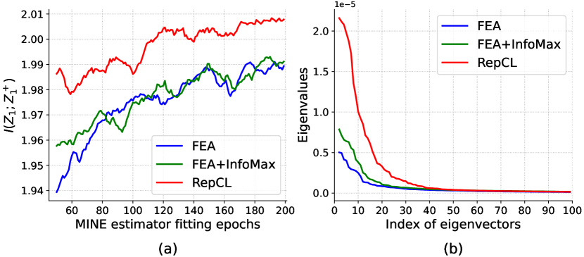
Figure 3: (a) MI estimator fitting curves of $I\left(Z_{1};Z^{+}_{1}\right)$ of test set in $\mathcal{T}_{1}$ of FewRel. (b) Distributions of eigenvalue for the representations learned by baselines and RepCL on $\mathcal{T}_{1}$ of FewRel. Top-100 largest eigenvalues are shown.

The results are shown in Table 4 and Figure 3(a). Both FEA+InfoMax and RepCL have higher $I(X_{1};Z_{1})$ than FEA baseline, showing that they can learn more sufficient representations. However, compared with RepCL, FEA+InfoMax has a lower $I(Z_{1};Z_{1}^{+})$ and worse final accuracy, indicating the InfoMax objective will introduce task-irrelevant information and lead to worse generalization. In contrast, $I(Z_{1};Z_{1}^{+})$ and final accuracy of RepCL are higher than those of two baselines, demonstrating that our method can capture more class-relevant features and better alleviate representation bias.

Additionally, Zhu et al. (2021) observed that representations with larger eigenvalues transfer better and suffer less forgetting. Therefore, in Figure 3(b), we also illustrate the distributions of eigenvalue for the representations learned in $\mathcal{T}_{1}$ of FewRel. As shown, the eigenvalues of RepCL are higher than two baselines, which also demonstrates that our method can learn effective representations for CL.

7.3 Influence of Memory Size

Memory size is the number of memorized instances for each class, which is an important factor for the performance of replay-based CL methods. Therefore, in this section, we study the impact of memory size on RepCL. We compare the performance of RepCL with ACA and FEA on FewRel under three memory sizes, 5, 10 and 20.

As shown in Table 5: (i) RepCL outperforms strong baselines under all three different memory sizes. Surprisingly, the performance of RepCL with $\mathcal{M}$=10 even defeats baselines with $\mathcal{M}$=20, showing the superior performance of our method. (ii) RepCL consistently increases performance than FEA, the two-stage training backbone of our method. Specifically, RepCL outperforms FEA by $1.5$, $1.3$ and $1.4$ in accuracy when the memory size is $5$, $10$, $20$, which indicates that our methods can reduce the dependence on the memory size.

Models	$\mathcal{M}$=5	$\mathcal{M}$=10	$\mathcal{M}$=20
FEA	81.8	84.3	85.0
ACA	82.7	84.7	85.5
RepCL	83.3	85.6	86.4

Table 5: Model performance on FewRel under different memory sizes. Our method has lighter dependence on memory size.

8 Conclusion

In this paper, we focus on continual learning for text classification in the class-incremental setting. We formally analyze the representation bias problem in continual learning from an information bottleneck perspective and find that learning more class-relevant features could alleviate the bias. Based on our analysis, we propose RepCL, which exploits both contrastive and generative representation learning objectives to capture more class-relevant features, and uses adversarial replay to better recover old knowledge. Extensive experiments on three tasks show that RepCL learns effective representations and significantly outperforms the latest baselines.

Limitations

Our paper has several limitations: (i) Our proposed RepCL utilizes contrastive and generative objectives to learn class-relevant representations, which introduces extra computational overhead and is less efficient than other replay-based CL methods; (ii) We only focus on catastrophic forgetting problem in continual text classification. How to encourage knowledge transfer in CL is not explored in this paper.

Ethics Statement

Our work complies with the ACL Ethics Policy. As text classification is a standard task in NLP and all datasets we used are public, we do not see any critical ethical considerations.

Appendix A Details about SupInfoNCE

A.1 Connection with InfoNCE

InfoNCE (van den Oord et al., 2018) is commonly used in multi-view contrastive representation learning as a proxy to approximate mutual information:

where $f$ is the encoder, $x^{+}$ is a positive view of $x$, $x^{-}$ is negative instance sampled from the whole input space $q(x^{-})$, $x^{-}\neq x_{i}^{+}$, and $\tau$ is the temperature hyperparameter.

In Section 4.3, we propose to maximize the MI between representations of instances from the same class. Under our scenario, a batch may contain several positive samples with the same label as the anchor sample. Since vanilla InfoNCE loss only considers the case of only one positive sample, it should be adapted to a multiple-positive version. Barbano et al. (2022) derive a multiple-positive extension of InfoNCE, SupInfoNCE:

where $x_{i}^{+}$ is a positive instance with the same label as $x$ in current batch.

Although both InfoNCE and SupInfoNCE are lower bounds of mutual information, due to the difference of positive instances, they are actually approximating difference objectives. For InfoNCE, since $x^{+}$ is another view of instance $x$, it will pull representations of the same instance together and push apart representations of all other instances and optimizing InfoNCE is maximizing the lower bound of MI $I(X;Z)$ between input and representation (Poole et al., 2019). In contrast, $x^{+}_{i}$ and $x$ in SupInfoNCE are instances from the same class, optimizing $I(Z;Z^{+})$ is pulling representations of instances of the same class together, which instructs the model capture more class-relevant features.

A.2 Comparison with SupCon

Previous work (Zhao et al., 2022) uses SupCon (Khosla et al., 2020), a popular supervised contrastive loss, to conduct contrastive learning:

However, Barbano et al. (2022) find that SupCon contains a non-contrastive constraint on the positive samples, which may harm the representation learning performance. Moreover, the connection between SupCon and mutual information has not been well studied. Therefore, we use SupInfoNCE instead.

Appendix B Details about FreeLB

In memory replay stage, to alleviate the overfitting on memorized instances, we introduce FreeLB (Zhu et al., 2020) adversarial loss:

where $F$ is the text classification model and $(x,y)$ is a batch of data from the memory bank $\mathcal{M}$, $\delta$ is the perturbation constrained within the $\epsilon$-ball, $K$ is step size hyperparameter. The inner maximization problem in (16) is to find the worst-case adversarial examples to maximize the training loss, while the outer minimization problem in (16) aims at optimizing the model to minimize the loss of adversarial examples. The inner maximization problem is solved iteratively in FreeLB:

$$\nabla(\delta_{t-1})=\nabla_{\delta}\mathcal{L}\left(F(x+\delta_{t-1}),y\right),$$ (17)

$$\delta_{t}=\prod_{\|\delta\|\leq\epsilon}\left(\delta_{t-1}+\alpha\cdot\frac{\nabla(\delta_{t-1})}{\|\nabla(\delta_{t-1})\|}\right),$$ (18)

where $\delta_{t}$ is the perturbation in $t$-th step and $\prod_{\|\delta\|\leq\epsilon}(\cdot)$ projects the perturbation onto the $\epsilon$-ball, $\alpha$ is step size.

Intuitively, FreeLB performs multiple adversarial attack iterations to craft adversarial examples, and simultaneously accumulates the free parameter gradients $\nabla_{\theta}\mathcal{L}$ in each iteration. After that, the model parameter $\theta$ is updated all at once with the accumulated gradients, which is equivalent to replacing the original batch with a $K$-times larger adversarial augmented batch.

Appendix C Dataset Details

FewRel

(Han et al., 2018) It is a large scale relation extraction dataset containing 80 relations. FewRel is a balanced dataset and each relation has 700 instances. Following Zhao et al. (2022); Wang et al. (2022b), we merge the original train and valid set of FewRel and for each relation we sample 420 instances for training and 140 instances for test. FewRel is licensed under MIT License.

TACRED

(Zhang et al., 2017) It is a crowdsourcing relation extraction dataset containing 42 relations (including no_relation) and 106264 instances. Following Zhao et al. (2022); Wang et al. (2022b), we remove no_relation and in our experiments. Since TACRED is a imbalanced dataset, for each relation the number of training instances is limited to 320 and the number of test instances is limited to 40. TACRED is licensed under LDC User Agreement for Non-Members.

MAVEN

(Wang et al., 2020) It is a large scale event detection dataset with 168 event types. Since MAVEN has a severe long-tail distribution, we use the data of the top 120 frequent classes. The original test set of MAVEN is not publicly available, and we use the original development set as our test set. MAVEN is licensed under Apache License 2.0.

HWU64

(Liu et al., 2019) It is an intent classification dataset with 64 intent classes. Following Liu et al. (2021), we use the data of the top 50 frequent classes and the total number of instances are 24137. HWU64 is licensed under CC-BY-4.0 License.

Appendix D Forgetting Rate

Followed Chaudhry et al. (2018), forgetting for a particular task is defined as the difference between the maximum knowledge gained about the task throughout the learning process in the past and the knowledge the model currently has about it. More concretely, for a classification problem, after training on task $j$, we denote $a_{j,i}$ as the accuracy evaluated on the test set of task $i\leq j$: Then the forgetting rate at $k$-th task is computed as:

$$f_{i}^{k}=\max_{l\in\{1,...,k-1\}}a_{l,i}-a_{k,i}$$ (19)

$$\mathrm{FR}_{k}=\frac{1}{k-1}\sum_{i=1}^{k-1}f_{i}^{k}.$$ (20)

We denote FR as the forgetting rate after finishing all tasks. Lower FR implies less forgetting on previous tasks.

Dataset	$\lambda_{1}$	$\lambda_{2}$	$Q$	$\tau$	$\eta$	$p_{\mathrm{xmlm}}$	$K$	$\alpha$	$\epsilon$
FewRel	0.05	0.2	512	0.05	0.99	0.5	2	0.1	0.2
TACRED	0.05	0.05	1024	0.1	0.99	0.2	2	0.1	0.2
MAVEN	0.05	0.05	512	0.05	0.99	0.1	2	0.1	0.2
HWU64	0.05	0.1	512	0.05	0.99	0.4	2	0.1	0.2

Table 6: Details of hyperparameters of RepCL in each dataset: contrastive loss weighting coefficient $\lambda_{1}$, XMLM loss coefficient $\lambda_{2}$, contrastive queue size $Q$, contrastive loss temperature $\tau$, exponential moving average decay rate $\eta$, masked proportion $p_{\mathrm{xmlm}}$, adversarial steps $K$, adversarial step size $\alpha$, adversarial maximum pertubation $\epsilon$.

Appendix E Baselines

IDBR (Huang et al., 2021) proposes an information disentanglement method to learn representations that can well generalize to future tasks. KCN (Cao et al., 2020) utilizes prototype retrospection and hierarchical distillation to consolidate knowledge. KDRK (Yu et al., 2021) encourages knowledge transfer between old and new classes. EMAR (Han et al., 2020) proposes a memory activation and reconsolidation mechanism to retain the learned knowledge. RP-CRE (Cui et al., 2021) proposes a memory network to retain the learned representations with class prototypes. CRL (Zhao et al., 2022) adopts contrastive learning replay and knowledge distillation to retain the learned knowledge. CRECL (Hu et al., 2022) uses a prototypical contrastive network to defy forgetting. FEA (Wang et al., 2022a) demonstrates the effectiveness of two-stage training framework, which can be seen as the backbone of RepCL. ACA (Wang et al., 2022b) designs two adversarial class augmentation mechanism to learn robust representations.

Appendix F Implementation Details

We implement RepCL with PyTorch (Paszke et al., 2019) and HuggingFace Transformers (Wolf et al., 2020). Following previous work Cui et al. (2021); Wang et al. (2022b, a), we use BERT_base (Devlin et al., 2019) as encoder. PyTorch is licensed under the modified BSD license. HuggingFace Transformers and BERT_base are licensed under the Apache License 2.0. Our use of existing artifacts is consistent with their intended use.

The text classification model can be seen as two parts: the BERT encoder $f_{\theta}$, and the MLP classifier $g_{\phi}$. Specifically, for the input $x$ in relation extraction, we use $[E_{11}],\ [E_{12}],\ [E_{21}]$ and $[E_{22}]$ to denote the start and end position of head and tail entity respectively, and the representation $z$ is the concatenation of the last hidden states of $[E_{11}]$ and $[E_{21}]$. For the input $x$ in event detection, the representation $z$ is the average pooling of the last hidden states of the trigger words. For the input $x$ in intent detection, the representation $z$ is the average pooling of the last hidden states of the whole sentence.

The learning rate of RepCL is set to 1e-5 for the BERT encoder and 1e-3 for the other layers. The training epochs for both the initial learning stage and the memory replay are 10. For FewRel, MAVEN and HWU64, the batch size is 32. For TACRED, the batch size is 16 because of the small amount of training data. The budget of memory bank for each class is 10 for all methods. We tune the hyperparameters of RepCL on the first three tasks for each dataset. Details of hyperparameter setting of RepCL are shown in Table 6. For all experiments, we use NVIDIA A40 and RTX 3090 GPUs and report the average result of 5 different task sequences.

Appendix G Full Experiment Results

The full experiment results on 10 continual learning tasks are shown in Table 7. As shown, RepCL consistently outperforms baselines in nearly all task stages on four datasets.

FewRel
Models	T1	T2	T3	T4	T5	T6	T7	T8	T9	T10	FR
IDBR (Huang et al., 2021)	97.9	91.9	86.8	83.6	80.6	77.7	75.6	73.7	71.7	68.9	30.4
KCN (Cao et al., 2020)	98.3	93.9	90.5	87.9	86.4	84.1	81.9	80.3	78.8	76.0	23.2
KDRK (Yu et al., 2021)	98.3	94.1	91.0	88.3	86.9	85.3	82.9	81.6	80.2	78.0	18.4
EMAR (Han et al., 2020)	98.1	94.3	92.3	90.5	89.7	88.5	87.2	86.1	84.8	83.6	12.1
RP-CRE (Cui et al., 2021)	97.8	94.7	92.1	90.3	89.4	88.0	87.1	85.8	84.4	82.8	10.3
CRL (Zhao et al., 2022)	98.2	94.6	92.5	90.5	89.4	87.9	86.9	85.6	84.5	83.1	11.5
CRECL (Hu et al., 2022)	97.8	94.9	92.7	90.9	89.4	87.5	85.7	84.6	83.6	82.7	11.6
FEA (Wang et al., 2022a)	98.3	94.8	93.1	91.7	90.8	89.1	87.9	86.8	85.8	84.3	8.9
ACA (Wang et al., 2022b)	98.3	95.0	92.6	91.3	90.4	89.2	87.6	87.0	86.3	84.7	11.0
RepCL	98.2	95.3	93.6	92.4	91.6	90.3	88.8	88.1	86.9	85.6	8.7
TACRED
Models	T1	T2	T3	T4	T5	T6	T7	T8	T9	T10	FR
IDBR (Huang et al., 2021)	97.9	91.1	83.1	76.5	74.2	70.5	66.6	64.2	63.8	60.1	35.3
KCN (Cao et al., 2020)	98.9	93.1	87.3	80.2	79.4	77.2	73.8	72.1	72.2	70.6	22.3
KDRK (Yu et al., 2021)	98.9	93.0	89.1	80.7	79.0	77.0	74.6	72.9	72.1	70.8	22.8
EMAR (Han et al., 2020)	98.3	92.0	87.4	84.1	82.1	80.6	78.3	76.6	76.8	76.1	20.0
RP-CRE (Cui et al., 2021)	97.5	92.2	89.1	84.2	81.7	81.0	78.1	76.1	75.0	75.3	17.5
CRL (Zhao et al., 2022)	97.7	93.2	89.8	84.7	84.1	81.3	80.2	79.1	79.0	78.0	18.0
CRECL (Hu et al., 2022)	96.6	93.1	89.7	87.8	85.6	84.3	83.6	81.4	79.3	78.5	16.3
FEA (Wang et al., 2022a)	97.6	92.6	89.5	86.4	84.8	82.8	81.0	78.5	78.5	77.7	13.3
ACA (Wang et al., 2022b)	98.0	92.1	90.6	85.5	84.4	82.2	80.0	78.6	78.8	78.1	13.8
RepCL	98.0	93.3	91.7	87.8	85.4	83.6	81.5	79.9	79.8	78.6	12.0
MAVEN
Models	T1	T2	T3	T4	T5	T6	T7	T8	T9	T10	FR
IDBR (Huang et al., 2021)	96.5	85.3	79.4	76.3	74.2	69.8	67.5	64.4	60.2	57.3	34.2
KCN (Cao et al., 2020)	97.2	87.7	83.2	80.3	77.9	75.1	71.9	68.4	67.7	64.4	29.0
KDRK (Yu et al., 2021)	97.2	88.6	84.3	81.6	78.1	75.8	72.5	69.6	68.9	65.4	28.3
EMAR (Han et al., 2020)	97.2	91.4	88.3	86.1	83.6	81.2	79.0	76.8	75.7	73.2	14.6
RP-CRE (Cui et al., 2021)	96.6	92.1	88.6	86.7	83.9	82.0	79.4	77.2	77.0	74.8	11.4
CRL (Zhao et al., 2022)	96.0	90.7	87.1	84.8	82.9	80.7	78.7	76.8	75.9	73.7	11.2
CRECL (Hu et al., 2022)	96.9	91.4	86.9	84.8	82.4	80.4	77.5	75.9	75.1	73.5	13.8
FEA (Wang et al., 2022a)	97.2	92.0	88.6	86.2	84.4	82.1	79.7	78.0	77.0	75.0	12.8
RepCL	97.1	92.2	88.9	86.7	84.8	82.5	80.4	78.4	77.7	75.9	10.7
HWU64
Models	T1	T2	T3	T4	T5	T6	T7	T8	T9	T10	FR
IDBR (Huang et al., 2021)	96.3	93.2	88.1	86.5	84.6	82.5	82.1	80.2	78.0	76.2	19.0
KCN (Cao et al., 2020)	98.6	94.0	90.7	90.4	87.0	84.9	84.4	83.7	82.7	81.9	13.5
KDRK (Yu et al., 2021)	98.6	94.5	91.2	90.4	87.3	86.0	85.8	85.1	82.5	81.4	14.0
EMAR (Han et al., 2020)	98.4	94.4	91.4	89.5	88.2	86.3	86.2	85.5	83.9	83.1	9.3
RP-CRE (Cui et al., 2021)	97.6	93.7	90.1	88.6	86.5	86.3	85.1	84.5	83.8	82.7	10.9
CRL (Zhao et al., 2022)	98.2	92.8	88.8	86.5	84.1	82.4	82.8	83.1	81.3	81.5	9.9
CRECL (Hu et al., 2022)	97.3	93.0	87.5	86.1	84.1	83.0	83.1	83.1	81.9	81.1	9.8
FEA (Wang et al., 2022a)	96.5	94.4	90.0	89.7	88.3	87.2	86.0	85.4	84.0	83.3	8.8
RepCL	97.7	93.7	91.5	89.9	88.9	87.4	87.5	87.0	84.9	84.8	8.0

Table 7: Accuracy (Acc, %) on all observed classes at at the stage of learning current task and forgetting rate (FR) after learning all tasks. Note some baselines are originally proposed to tackle one specific task. We adapt these baselines on other tasks and report the corresponding results. RepCL consistently outperforms baselines in nearly all task stages on four datasets.

References

- Achille and Soatto (2018) Alessandro Achille and Stefano Soatto. 2018. Emergence of invariance and disentanglement in deep representations. J. Mach. Learn. Res., 19:50:1–50:34.
- Aljundi et al. (2018) Rahaf Aljundi, Francesca Babiloni, Mohamed Elhoseiny, Marcus Rohrbach, and Tinne Tuytelaars. 2018. Memory aware synapses: Learning what (not) to forget. In Computer Vision - ECCV 2018 - 15th European Conference, Munich, Germany, September 8-14, 2018, Proceedings, Part III, volume 11207 of Lecture Notes in Computer Science, pages 144–161. Springer.
- Barbano et al. (2022) Carlo Alberto Barbano, Benoit Dufumier, Enzo Tartaglione, Marco Grangetto, and Pietro Gori. 2022. Unbiased supervised contrastive learning. CoRR, abs/2211.05568.
- Belghazi et al. (2018) Ishmael Belghazi, Sai Rajeswar, Aristide Baratin, R. Devon Hjelm, and Aaron C. Courville. 2018. MINE: mutual information neural estimation. CoRR, abs/1801.04062.
- Biesialska et al. (2020) Magdalena Biesialska, Katarzyna Biesialska, and Marta R. Costa-jussà. 2020. Continual lifelong learning in natural language processing: A survey. In Proceedings of the 28th International Conference on Computational Linguistics, COLING 2020, Barcelona, Spain (Online), December 8-13, 2020, pages 6523–6541. International Committee on Computational Linguistics.
- Buzzega et al. (2020) Pietro Buzzega, Matteo Boschini, Angelo Porrello, Davide Abati, and Simone Calderara. 2020. Dark experience for general continual learning: a strong, simple baseline. In Advances in Neural Information Processing Systems 33: Annual Conference on Neural Information Processing Systems 2020, NeurIPS 2020, December 6-12, 2020, virtual.
- Cao et al. (2020) Pengfei Cao, Yubo Chen, Jun Zhao, and Taifeng Wang. 2020. Incremental event detection via knowledge consolidation networks. In Proceedings of the 2020 Conference on Empirical Methods in Natural Language Processing (EMNLP), pages 707–717, Online. Association for Computational Linguistics.
- Cao et al. (2022) Rui Cao, Yihao Wang, Yuxin Liang, Ling Gao, Jie Zheng, Jie Ren, and Zheng Wang. 2022. Exploring the impact of negative samples of contrastive learning: A case study of sentence embedding. In Findings of the Association for Computational Linguistics: ACL 2022, pages 3138–3152, Dublin, Ireland. Association for Computational Linguistics.
- Cha et al. (2021) Hyuntak Cha, Jaeho Lee, and Jinwoo Shin. 2021. Col: Contrastive continual learning. In 2021 IEEE/CVF International Conference on Computer Vision, ICCV 2021, Montreal, QC, Canada, October 10-17, 2021, pages 9496–9505. IEEE.
- Chaudhry et al. (2018) Arslan Chaudhry, Puneet Kumar Dokania, Thalaiyasingam Ajanthan, and Philip H. S. Torr. 2018. Riemannian walk for incremental learning: Understanding forgetting and intransigence. In Computer Vision - ECCV 2018 - 15th European Conference, Munich, Germany, September 8-14, 2018, Proceedings, Part XI, volume 11215 of Lecture Notes in Computer Science, pages 556–572. Springer.
- Cui et al. (2021) Li Cui, Deqing Yang, Jiaxin Yu, Chengwei Hu, Jiayang Cheng, Jingjie Yi, and Yanghua Xiao. 2021. Refining sample embeddings with relation prototypes to enhance continual relation extraction. In Proceedings of the 59th Annual Meeting of the Association for Computational Linguistics and the 11th International Joint Conference on Natural Language Processing (Volume 1: Long Papers), pages 232–243, Online. Association for Computational Linguistics.
- Devlin et al. (2019) Jacob Devlin, Ming-Wei Chang, Kenton Lee, and Kristina Toutanova. 2019. BERT: Pre-training of deep bidirectional transformers for language understanding. In Proceedings of the 2019 Conference of the North American Chapter of the Association for Computational Linguistics: Human Language Technologies, Volume 1 (Long and Short Papers), pages 4171–4186, Minneapolis, Minnesota. Association for Computational Linguistics.
- Gao et al. (2021) Tianyu Gao, Xingcheng Yao, and Danqi Chen. 2021. SimCSE: Simple contrastive learning of sentence embeddings. In Proceedings of the 2021 Conference on Empirical Methods in Natural Language Processing, pages 6894–6910, Online and Punta Cana, Dominican Republic. Association for Computational Linguistics.
- Guo et al. (2022) Yiduo Guo, Bing Liu, and Dongyan Zhao. 2022. Online continual learning through mutual information maximization. In International Conference on Machine Learning, ICML 2022, 17-23 July 2022, Baltimore, Maryland, USA, volume 162 of Proceedings of Machine Learning Research, pages 8109–8126. PMLR.
- Han et al. (2020) Xu Han, Yi Dai, Tianyu Gao, Yankai Lin, Zhiyuan Liu, Peng Li, Maosong Sun, and Jie Zhou. 2020. Continual relation learning via episodic memory activation and reconsolidation. In Proceedings of the 58th Annual Meeting of the Association for Computational Linguistics, pages 6429–6440, Online. Association for Computational Linguistics.
- Han et al. (2018) Xu Han, Hao Zhu, Pengfei Yu, Ziyun Wang, Yuan Yao, Zhiyuan Liu, and Maosong Sun. 2018. FewRel: A large-scale supervised few-shot relation classification dataset with state-of-the-art evaluation. In Proceedings of the 2018 Conference on Empirical Methods in Natural Language Processing, pages 4803–4809, Brussels, Belgium. Association for Computational Linguistics.
- He et al. (2020) Kaiming He, Haoqi Fan, Yuxin Wu, Saining Xie, and Ross B. Girshick. 2020. Momentum contrast for unsupervised visual representation learning. In 2020 IEEE/CVF Conference on Computer Vision and Pattern Recognition, CVPR 2020, Seattle, WA, USA, June 13-19, 2020, pages 9726–9735. Computer Vision Foundation / IEEE.
- Hu et al. (2022) Chengwei Hu, Deqing Yang, Haoliang Jin, Zhen Chen, and Yanghua Xiao. 2022. Improving continual relation extraction through prototypical contrastive learning. In Proceedings of the 29th International Conference on Computational Linguistics, pages 1885–1895, Gyeongju, Republic of Korea. International Committee on Computational Linguistics.
- Huang et al. (2021) Yufan Huang, Yanzhe Zhang, Jiaao Chen, Xuezhi Wang, and Diyi Yang. 2021. Continual learning for text classification with information disentanglement based regularization. In Proceedings of the 2021 Conference of the North American Chapter of the Association for Computational Linguistics: Human Language Technologies, pages 2736–2746, Online. Association for Computational Linguistics.
- Khosla et al. (2020) Prannay Khosla, Piotr Teterwak, Chen Wang, Aaron Sarna, Yonglong Tian, Phillip Isola, Aaron Maschinot, Ce Liu, and Dilip Krishnan. 2020. Supervised contrastive learning. In Advances in Neural Information Processing Systems 33: Annual Conference on Neural Information Processing Systems 2020, NeurIPS 2020, December 6-12, 2020, virtual.
- Kirkpatrick et al. (2017) James Kirkpatrick, Razvan Pascanu, Neil Rabinowitz, Joel Veness, Guillaume Desjardins, Andrei A Rusu, Kieran Milan, John Quan, Tiago Ramalho, Agnieszka Grabska-Barwinska, et al. 2017. Overcoming catastrophic forgetting in neural networks. Proceedings of the national academy of sciences, 114(13):3521–3526.
- Lange et al. (2022) Matthias De Lange, Rahaf Aljundi, Marc Masana, Sarah Parisot, Xu Jia, Ales Leonardis, Gregory G. Slabaugh, and Tinne Tuytelaars. 2022. A continual learning survey: Defying forgetting in classification tasks. IEEE Trans. Pattern Anal. Mach. Intell., 44(7):3366–3385.
- Liu et al. (2021) Qingbin Liu, Xiaoyan Yu, Shizhu He, Kang Liu, and Jun Zhao. 2021. Lifelong intent detection via multi-strategy rebalancing. CoRR, abs/2108.04445.
- Liu et al. (2019) Xingkun Liu, Arash Eshghi, Pawel Swietojanski, and Verena Rieser. 2019. Benchmarking natural language understanding services for building conversational agents. In Increasing Naturalness and Flexibility in Spoken Dialogue Interaction - 10th International Workshop on Spoken Dialogue Systems, IWSDS 2019, Syracuse, Sicily, Italy, 24-26 April 2019, volume 714 of Lecture Notes in Electrical Engineering, pages 165–183. Springer.
- Mai et al. (2022) Zheda Mai, Ruiwen Li, Jihwan Jeong, David Quispe, Hyunwoo Kim, and Scott Sanner. 2022. Online continual learning in image classification: An empirical survey. Neurocomputing, 469:28–51.
- Mallya and Lazebnik (2018) Arun Mallya and Svetlana Lazebnik. 2018. Packnet: Adding multiple tasks to a single network by iterative pruning. In 2018 IEEE Conference on Computer Vision and Pattern Recognition, CVPR 2018, Salt Lake City, UT, USA, June 18-22, 2018, pages 7765–7773. Computer Vision Foundation / IEEE Computer Society.
- Paszke et al. (2019) Adam Paszke, Sam Gross, Francisco Massa, Adam Lerer, James Bradbury, Gregory Chanan, Trevor Killeen, Zeming Lin, Natalia Gimelshein, Luca Antiga, Alban Desmaison, Andreas Köpf, Edward Z. Yang, Zachary DeVito, Martin Raison, Alykhan Tejani, Sasank Chilamkurthy, Benoit Steiner, Lu Fang, Junjie Bai, and Soumith Chintala. 2019. Pytorch: An imperative style, high-performance deep learning library. In Advances in Neural Information Processing Systems 32: Annual Conference on Neural Information Processing Systems 2019, NeurIPS 2019, December 8-14, 2019, Vancouver, BC, Canada, pages 8024–8035.
- Poole et al. (2019) Ben Poole, Sherjil Ozair, Aäron van den Oord, Alexander A. Alemi, and G. Tucker. 2019. On variational bounds of mutual information. In International Conference on Machine Learning.
- Prabhu et al. (2020) Ameya Prabhu, Philip H. S. Torr, and Puneet K. Dokania. 2020. Gdumb: A simple approach that questions our progress in continual learning. In Computer Vision - ECCV 2020 - 16th European Conference, Glasgow, UK, August 23-28, 2020, Proceedings, Part II, volume 12347 of Lecture Notes in Computer Science, pages 524–540. Springer.
- Rebuffi et al. (2017) Sylvestre-Alvise Rebuffi, Alexander Kolesnikov, Georg Sperl, and Christoph H. Lampert. 2017. icarl: Incremental classifier and representation learning. In 2017 IEEE Conference on Computer Vision and Pattern Recognition, CVPR 2017, Honolulu, HI, USA, July 21-26, 2017, pages 5533–5542. IEEE Computer Society.
- Shwartz-Ziv and Tishby (2017) Ravid Shwartz-Ziv and Naftali Tishby. 2017. Opening the black box of deep neural networks via information. CoRR, abs/1703.00810.
- Sun et al. (2020) Fan-Keng Sun, Cheng-Hao Ho, and Hung-Yi Lee. 2020. LAMOL: language modeling for lifelong language learning. In 8th International Conference on Learning Representations, ICLR 2020, Addis Ababa, Ethiopia, April 26-30, 2020. OpenReview.net.
- Tian et al. (2020) Yonglong Tian, Chen Sun, Ben Poole, Dilip Krishnan, Cordelia Schmid, and Phillip Isola. 2020. What makes for good views for contrastive learning? In Advances in Neural Information Processing Systems 33: Annual Conference on Neural Information Processing Systems 2020, NeurIPS 2020, December 6-12, 2020, virtual.
- Tishby et al. (2000) Naftali Tishby, Fernando C. N. Pereira, and William Bialek. 2000. The information bottleneck method. CoRR, physics/0004057.
- Tishby and Zaslavsky (2015) Naftali Tishby and Noga Zaslavsky. 2015. Deep learning and the information bottleneck principle. In 2015 IEEE Information Theory Workshop, ITW 2015, Jerusalem, Israel, April 26 - May 1, 2015, pages 1–5. IEEE.
- van den Oord et al. (2018) Aäron van den Oord, Yazhe Li, and Oriol Vinyals. 2018. Representation learning with contrastive predictive coding. CoRR, abs/1807.03748.
- Wang et al. (2019) Hong Wang, Wenhan Xiong, Mo Yu, Xiaoxiao Guo, Shiyu Chang, and William Yang Wang. 2019. Sentence embedding alignment for lifelong relation extraction. In Proceedings of the 2019 Conference of the North American Chapter of the Association for Computational Linguistics: Human Language Technologies, Volume 1 (Long and Short Papers), pages 796–806, Minneapolis, Minnesota. Association for Computational Linguistics.
- Wang et al. (2022a) Peiyi Wang, Yifan Song, Tianyu Liu, Rundong Gao, Binghuai Lin, Yunbo Cao, and Zhifang Sui. 2022a. Less is more: Rethinking state-of-the-art continual relation extraction models with a frustratingly easy but effective approach. arXiv preprint arXiv:2209.00243.
- Wang et al. (2022b) Peiyi Wang, Yifan Song, Tianyu Liu, Binghuai Lin, Yunbo Cao, Sujian Li, and Zhifang Sui. 2022b. Learning robust representations for continual relation extraction via adversarial class augmentation. CoRR, abs/2210.04497.
- Wang et al. (2020) Xiaozhi Wang, Ziqi Wang, Xu Han, Wangyi Jiang, Rong Han, Zhiyuan Liu, Juanzi Li, Peng Li, Yankai Lin, and Jie Zhou. 2020. MAVEN: A Massive General Domain Event Detection Dataset. In Proceedings of the 2020 Conference on Empirical Methods in Natural Language Processing (EMNLP), pages 1652–1671, Online. Association for Computational Linguistics.
- Wolf et al. (2020) Thomas Wolf, Lysandre Debut, Victor Sanh, Julien Chaumond, Clement Delangue, Anthony Moi, Pierric Cistac, Tim Rault, Remi Louf, Morgan Funtowicz, Joe Davison, Sam Shleifer, Patrick von Platen, Clara Ma, Yacine Jernite, Julien Plu, Canwen Xu, Teven Le Scao, Sylvain Gugger, Mariama Drame, Quentin Lhoest, and Alexander Rush. 2020. Transformers: State-of-the-art natural language processing. In Proceedings of the 2020 Conference on Empirical Methods in Natural Language Processing: System Demonstrations, pages 38–45, Online. Association for Computational Linguistics.
- Wu and Zhao (2022) Bohong Wu and Hai Zhao. 2022. Sentence representation learning with generative objective rather than contrastive objective. CoRR, abs/2210.08474.
- Wu et al. (2022) Tongtong Wu, Massimo Caccia, Zhuang Li, Yuan-Fang Li, Guilin Qi, and Gholamreza Haffari. 2022. Pretrained language model in continual learning: A comparative study. In The Tenth International Conference on Learning Representations, ICLR 2022, Virtual Event, April 25-29, 2022. OpenReview.net.
- Xia et al. (2023) Heming Xia, Peiyi Wang, Tianyu Liu, Binghuai Lin, Yunbo Cao, and Zhifang Sui. 2023. Enhancing continual relation extraction via classifier decomposition. arXiv preprint arXiv:2305.04636.
- Yang et al. (2021) Ziyi Yang, Yinfei Yang, Daniel Cer, Jax Law, and Eric Darve. 2021. Universal sentence representation learning with conditional masked language model. In Proceedings of the 2021 Conference on Empirical Methods in Natural Language Processing, pages 6216–6228, Online and Punta Cana, Dominican Republic. Association for Computational Linguistics.
- Yu et al. (2021) Pengfei Yu, Heng Ji, and Prem Natarajan. 2021. Lifelong event detection with knowledge transfer. In Proceedings of the 2021 Conference on Empirical Methods in Natural Language Processing, pages 5278–5290, Online and Punta Cana, Dominican Republic. Association for Computational Linguistics.
- Zhang et al. (2017) Yuhao Zhang, Victor Zhong, Danqi Chen, Gabor Angeli, and Christopher D. Manning. 2017. Position-aware attention and supervised data improve slot filling. In Proceedings of the 2017 Conference on Empirical Methods in Natural Language Processing, pages 35–45, Copenhagen, Denmark. Association for Computational Linguistics.
- Zhao et al. (2022) Kang Zhao, Hua Xu, Jiangong Yang, and Kai Gao. 2022. Consistent representation learning for continual relation extraction. In Findings of the Association for Computational Linguistics: ACL 2022, pages 3402–3411, Dublin, Ireland. Association for Computational Linguistics.
- Zhu et al. (2020) Chen Zhu, Yu Cheng, Zhe Gan, Siqi Sun, Tom Goldstein, and Jingjing Liu. 2020. Freelb: Enhanced adversarial training for natural language understanding. In 8th International Conference on Learning Representations, ICLR 2020, Addis Ababa, Ethiopia, April 26-30, 2020. OpenReview.net.
- Zhu et al. (2021) Fei Zhu, Zhen Cheng, Xu-Yao Zhang, and Chenglin Liu. 2021. Class-incremental learning via dual augmentation. In Advances in Neural Information Processing Systems 34: Annual Conference on Neural Information Processing Systems 2021, NeurIPS 2021, December 6-14, 2021, virtual, pages 14306–14318.