Direct Shaping of Minimum and Maximum Singular Values: An $\mathcal{H}_{-}/\mathcal{H}_{\infty}$ Synthesis Approach for Fault Detection Filters

Abstract

The performance of fault detection filters relies on a high sensitivity to faults and a low sensitivity to disturbances. The aim of this paper is to develop an approach to directly shape these sensitivities, expressed in terms of minimum and maximum singular values. The developed method offers an alternative solution to the $\mathcal{H}_{-}/\mathcal{H}_{\infty}$ synthesis problem, building upon traditional multiobjective synthesis results. The result is an optimal filter synthesized via iterative convex optimization and the approach is particularly useful for fault diagnosis as illustrated by a numerical example.

1 Introduction

Fault detection and isolation (FDI) is highly important in many control applications which are becoming increasingly more demanding and more complex. In particular, FDI is important for the high-tech production industry which is shifting towards predictive maintenance strategies. This paradigm shift is motivated as a result of the high costs associated with unscheduled downtime. In this context, real-time fault diagnosis of complex closed-loop controlled multi-input multi-output (MIMO) systems is the foundation for effective targeted maintenance and optimal scheduling of downtime.

It is commonly recognized that satisfactory performance of model-based FDI systems is only achievable by a balanced trade-off. Techniques based on $\mathcal{H}_{\infty}$ optimization and $\mu$ design have been developed and applied, see, e.g., Sadrnia et al. (1997); Ding et al. (2000); Zhong et al. (2003). However, these $\mathcal{H}_{\infty}$ approaches do not directly account for this trade-off as $\mathcal{H}_{\infty}$ is only a measure for maximum gain. Apart from rejecting disturbance, noise and being insensitive to model uncertainties, the fault diagnosis system needs to be as sensitive to faults as possible. Hence, fault sensitivity needs to be addressed explicitly during design.

One way to enforce sensitivity to faults is to reformulate the problem, see Henry (2021), or by reformulating the problem as a fault estimation problem, see Stoustrup and H. Niemann (2002). In this way, the problem can still be solved as a fictitious $\mathcal{H}_{\infty}$ problem, however, undesired conservatism may be introduced. Alternatively, more direct $\mathcal{H}_{-}/\mathcal{H}_{\infty}$ approaches are attractive as the trade-off is explicitly embedded in the problem formulation. $\mathcal{H}_{-}/\mathcal{H}_{\infty}$ filter design can be pursued via factorization approaches as in Ding et al. (2000), or, e.g., via Riccati equations, see Liu and Zhou (2007). In particular LMI formulations are of interest due to the relative ease to incorporate additional design objectives, see Wang et al. (2007); Hou and Patton (1996). In addition, LMI methods are well established for controller synthesis and observer design as demonstrated in Scherer et al. (1997); Scherer and Weiland (2020). However, these methods are not specifically tailored to FDI problems.

Although important progress has been made in fault detection for complex engineered systems, at present accurate FDI for complex systems is hampered by lack of compatible synthesis tools. The aim of this paper is to develop an alternative $\mathcal{H}_{-}/\mathcal{H}_{\infty}$ synthesis algorithm, building upon traditional multiobjective synthesis results originating from controller design. The theory builds upon the notion of minimum gain and allows to directly shape the minimum and maximum singular values of the complete system. Hence, the contribution of this paper is twofold: 1) Development of an alternative approach for FDI design, 2) Development of the associated synthesis problem.

This paper is organized as follows. The paper proceeds with notation and the required preliminaries, listed in Section 2. The underlying subproblem for multiobjective filter design is presented in a generic manner in Section 3. Subsequently, the design specifications for fault diagnosis filter design, the relevant matrix inequalities, and its synthesis procedure are described in Section 4. A numerical fault diagnosis case study, presented in Section 5, illustrates the effectiveness of the proposed approach and finally, a conclusion is drawn in Section 6.

2 Preliminaries

2.1 Notation

Positive definiteness and positive semidefiniteness of a matrix $A$ are denoted by $A\succ 0$ and $A\succeq 0$, respectively. Similarly, $A\prec 0$ and $A\preceq 0$ denote negative definite and negative semidefinite matrices, respectively. The sets of all nonnegative and positive integers are denoted $\mathbb{N}$ and $\mathbb{N}_{\geq 0}$. The sets of real numbers and nonnegative real numbers are indicated by $\mathbb{R}$ and $\mathbb{R}_{\geq 0}$. The set of $n$ by $n$ symmetric matrices is denoted as $\mathbb{S}^{n}$. By $\left\lVert\cdot\right\rVert$ the Euclidean norm is defined. Repeated blocks within symmetric matrices are replaced by $*$ for brevity and clarity. The identity matrix is written as $I$ and a matrix of zeros is written as $0$. The maximum and minimum singular values of the matrix $A$ are denoted by $\bar{\sigma}(A)$ and $\underline{\sigma}(A)$, respectively. The real rational subspace of $\mathcal{H}_{\infty}$ is denoted by $\mathcal{RH}_{\infty}$. $y\in\mathcal{L}_{2}$ if $\left\lVert y\right\rVert_{2}^{2}=\int_{0}^{\infty}y^{\top}(t)y(t)\mathrm{d}t<\infty$. $y\in\mathcal{L}_{2e}$ if $\left\lVert y\right\rVert_{2T}^{2}=\int_{0}^{T}y^{\top}(t)y(t)\mathrm{d}t<\infty$, $T\in\mathbb{R}_{\geq 0}$.

2.2 Minimum and Maximum Gain

Lemma 1

Minimum gain (Liu and Zhou (2007); Wang et al. (2007)) The smallest gain of the continuous-time LTI system $G:\mathcal{L}_{2e}\rightarrow\mathcal{L}_{2e}$, that is the $\mathcal{H}_{-}$ index, is defined as

$$\left\lVert G\right\rVert_{-}=\inf_{\omega\in\mathbb{R}_{\geq 0}}\underline{\sigma}(G(j\omega)).$$ (1)

The minimum gain is not a norm and therefor named the $\mathcal{H}_{-}$ index.

Definition 1

Maximum gain (Skogestad and Postlethwaite (2001)) The $\mathcal{H}_{\infty}$ norm of the continuous-time LTI system $G:\mathcal{L}_{2e}\rightarrow\mathcal{L}_{2e}$, denoted as $\left\lVert G\right\rVert_{\infty}$, is given by

$$\left\lVert G\right\rVert_{\infty}=\sup_{\omega\in\mathbb{R}_{\geq 0}}\bar{\sigma}(G(j\omega)).$$ (2)

Lemma 2

Minimum Gain Lemma (Bridgeman and Forbes (2015); Caverly (2018)) Consider a continuous-time LTI system $G:\mathcal{L}_{2e}\rightarrow\mathcal{L}_{2e}$, with state space realization $(\mathcal{A},\mathcal{B},\mathcal{C},\mathcal{D})$, where $\mathcal{A}\in\mathbb{R}^{n\times n}$, $\mathcal{B}\in\mathbb{R}^{n\times m}$, $\mathcal{C}\in\mathbb{R}^{p\times n}$, and $\mathcal{D}\in\mathbb{R}^{p\times m}$. The system $G$ has minimum gain $\nu$ under the following sufficient condition. There exists $X\in\mathbb{S}^{n}$ and $\nu\in\mathbb{R}_{\geq 0}$, where $X\succeq 0$, such that

$$\begin{bmatrix}X\mathcal{A}+\mathcal{A}^{\top}X-\mathcal{C}^{\top}\mathcal{C}&X\mathcal{B}-\mathcal{C}^{\top}\mathcal{D}&0\\ *&-\mathcal{D}^{\top}\mathcal{D}&\nu I\\ *&*&-I\end{bmatrix}\prec 0.$$ (3)

Lemma 3

Bounded Real Lemma (Gahinet and Apkarian (1994)) Consider a continuous-time LTI system $G:\mathcal{L}_{2e}\rightarrow\mathcal{L}_{2e}$, with state space realization $(\mathcal{A},\mathcal{B},\mathcal{C},\mathcal{D})$, where $\mathcal{A}\in\mathbb{R}^{n\times n}$, $\mathcal{B}\in\mathbb{R}^{n\times m}$, $\mathcal{C}\in\mathbb{R}^{p\times n}$, and $\mathcal{D}\in\mathbb{R}^{p\times m}$. The inequality $\left\lVert G\right\rVert_{\infty}<\gamma$ holds under the following necessary and sufficient conditions. There exists $X\in\mathbb{S}^{n}$ and $\gamma\in\mathbb{R}_{>0}$, where $X\succ 0$, such that

$$\begin{bmatrix}X\mathcal{A}+\mathcal{A}^{\top}X&X\mathcal{B}&\mathcal{C}^{\top}\\ *&-\gamma^{2}I&\mathcal{D}^{\top}\\ *&*&-I\end{bmatrix}\prec 0.$$ (4)

3 $\mathcal{H}_{-}/\mathcal{H}_{\infty}$ Approach to Fault Detection

This section introduces the generalized plant formulation and introduces the relevant notation for transformation of variables and objective channel selection. In addition, the underlying multiobjective synthesis subproblem is described.

3.1 General Closed-loop Interconnection

Consider the generalized plant $P$, as depicted in Figure 1,

Figure 1: Generalized plant $P:\begin{bmatrix}\tilde{w}^{\top}&\tilde{u}^{\top}\end{bmatrix}^{\top}\rightarrow\begin{bmatrix}\tilde{z}^{\top}&\tilde{y}^{\top}\end{bmatrix}^{\top}$ and filter $Q:\tilde{y}\rightarrow\tilde{u}$. The closed-loop system with performance channel $T:\tilde{w}\rightarrow\tilde{z}$ is highlighted in ( ).

with generalized disturbance channel $\tilde{w}$, generalized performance channel $\tilde{z}$, input $\tilde{u}$, and output $\tilde{y}$, which admits the state-space realization

$$\left[\begin{array}[]{c}\dot{x}\\ \hline\cr\tilde{z}\\ \tilde{y}\end{array}\right]=\left[\begin{array}[]{c|cc}A&B_{1}&B_{2}\\ \hline\cr C_{1}&D_{11}&D_{12}\\ C_{2}&D_{21}&D_{22}\end{array}\right]\left[\begin{array}[]{c}x\\ \hline\cr\tilde{w}\\ \tilde{u}\end{array}\right].$$ (5)

The to be designed filter $Q$ is any finite dimensional LTI system described as

$$\left[\begin{array}[]{c}\dot{x}_{c}\\ \tilde{u}\end{array}\right]=\left[\begin{array}[]{cc}{\color[rgb]{0,0,0}A_{c}}&{\color[rgb]{0,0,0}B_{c}}\\ {\color[rgb]{0,0,0}C_{c}}&{\color[rgb]{0,0,0}D_{c}}\end{array}\right]\left[\begin{array}[]{c}x_{c}\\ \tilde{y}\end{array}\right].$$ (6)

In particular, the state dimension of the filter $Q$, $x_{c}$, is not decided upon in advance. Let $T:\tilde{w}\rightarrow\tilde{z}$ denote the closed-loop transfer function, formed by the lower linear fractional transformation (LFT) between $P$ and $Q$. The closed-loop system $T=\mathcal{F}_{l}(P,Q)$, and admits the description

$$\dot{x}_{\mathrm{cl}} ={\color[rgb]{0,0,0}\mathcal{A}}x_{\mathrm{cl}}+{\color[rgb]{0,0,0}\mathcal{B}}\tilde{w},$$ (7a)

$$\tilde{z} ={\color[rgb]{0,0,0}\mathcal{C}}x_{\mathrm{cl}}+{\color[rgb]{0,0,0}\mathcal{D}}\tilde{w},$$ (7b)

where

$${\color[rgb]{0,0,0}\mathcal{A}} =\begin{bmatrix}A+B_{2}{\color[rgb]{0,0,0}D_{c}}{\color[rgb]{0,0,0}\bar{D}}C_{2}&B_{2}\left(I+{\color[rgb]{0,0,0}D_{c}}{\color[rgb]{0,0,0}\bar{D}}D_{22}\right){\color[rgb]{0,0,0}C_{c}}\\ {\color[rgb]{0,0,0}B_{c}}{\color[rgb]{0,0,0}\bar{D}}C_{2}&{\color[rgb]{0,0,0}A_{c}}+{\color[rgb]{0,0,0}B_{c}}{\color[rgb]{0,0,0}\bar{D}}D_{22}{\color[rgb]{0,0,0}C_{c}}\end{bmatrix},$$ (8a)

$${\color[rgb]{0,0,0}\mathcal{B}} =\begin{bmatrix}B_{1}+B_{2}{\color[rgb]{0,0,0}D_{c}}{\color[rgb]{0,0,0}\bar{D}}D_{21}\\ {\color[rgb]{0,0,0}B_{c}}{\color[rgb]{0,0,0}\bar{D}}D_{21}\end{bmatrix},$$ (8b)

$${\color[rgb]{0,0,0}\mathcal{C}} =\begin{bmatrix}C_{1}+D_{12}{\color[rgb]{0,0,0}D_{c}}{\color[rgb]{0,0,0}\bar{D}}C_{2}&D_{12}\left(I+{\color[rgb]{0,0,0}D_{c}}{\color[rgb]{0,0,0}\bar{D}}D_{22}\right){\color[rgb]{0,0,0}C_{c}}\end{bmatrix},$$ (8c)

$${\color[rgb]{0,0,0}\mathcal{D}} =D_{11}+D_{12}{\color[rgb]{0,0,0}D_{c}}{\color[rgb]{0,0,0}\bar{D}}D_{21},$$ (8d)

where ${\color[rgb]{0,0,0}\bar{D}}=\left(I-D_{22}{\color[rgb]{0,0,0}D_{c}}\right)^{-1}$.

3.2 Change of Variables

The system is nonlinear in ${\color[rgb]{0,0,0}A_{c}}$, ${\color[rgb]{0,0,0}B_{c}}$, ${\color[rgb]{0,0,0}C_{c}}$, and ${\color[rgb]{0,0,0}D_{c}}$. To obtain an affine relation, the following change of variables is deployed

$${\color[rgb]{0,0,0}A_{c2}} ={\color[rgb]{0,0,0}A_{c}}+{\color[rgb]{0,0,0}B_{c}}{\color[rgb]{0,0,0}\bar{D}}D_{22}{\color[rgb]{0,0,0}C_{c}},$$ (9a)

$${\color[rgb]{0,0,0}B_{c2}} ={\color[rgb]{0,0,0}B_{c}}{\color[rgb]{0,0,0}\bar{D}},$$ (9b)

$${\color[rgb]{0,0,0}C_{c2}} =\left(I+{\color[rgb]{0,0,0}D_{c}}{\color[rgb]{0,0,0}\bar{D}}D_{22}\right){\color[rgb]{0,0,0}C_{c}},$$ (9c)

$${\color[rgb]{0,0,0}D_{c2}} ={\color[rgb]{0,0,0}D_{c}}{\color[rgb]{0,0,0}\bar{D}},$$ (9d)

which renders the closed-loop system matrices

$${\color[rgb]{0,0,0}\mathcal{A}} =\begin{bmatrix}A+B_{2}{\color[rgb]{0,0,0}D_{c2}}C_{2}&B_{2}{\color[rgb]{0,0,0}C_{c2}}\\ {\color[rgb]{0,0,0}B_{c2}}C_{2}&{\color[rgb]{0,0,0}A_{c2}}\end{bmatrix},$$ (10a)

$${\color[rgb]{0,0,0}\mathcal{B}} =\begin{bmatrix}B_{1}+B_{2}{\color[rgb]{0,0,0}D_{c2}}D_{21}\\ {\color[rgb]{0,0,0}B_{c2}}D_{21}\end{bmatrix},$$ (10b)

$${\color[rgb]{0,0,0}\mathcal{C}} =\begin{bmatrix}C_{1}+D_{12}{\color[rgb]{0,0,0}D_{c2}}C_{2}&D_{12}{\color[rgb]{0,0,0}C_{c2}}\end{bmatrix},$$ (10c)

$${\color[rgb]{0,0,0}\mathcal{D}} =D_{11}+D_{11}+D_{12}{\color[rgb]{0,0,0}D_{c2}}D_{21},$$ (10d)

affine in ${\color[rgb]{0,0,0}A_{c2}}$, ${\color[rgb]{0,0,0}B_{c2}}$, ${\color[rgb]{0,0,0}C_{c2}}$, and ${\color[rgb]{0,0,0}D_{c2}}$. The reverse change of variables is

$${\color[rgb]{0,0,0}A_{c}} ={\color[rgb]{0,0,0}A_{c2}}-{\color[rgb]{0,0,0}B_{c2}}D_{22}\left(I+{\color[rgb]{0,0,0}D_{c2}}D_{22}\right)^{-1}{\color[rgb]{0,0,0}C_{c2}},$$ (11a)

$${\color[rgb]{0,0,0}B_{c}} ={\color[rgb]{0,0,0}B_{c2}}\left(I+D_{22}{\color[rgb]{0,0,0}D_{c2}}\right)^{-1},$$ (11b)

$${\color[rgb]{0,0,0}C_{c}} =\left(I+{\color[rgb]{0,0,0}D_{c2}}D_{22}\right)^{-1}{\color[rgb]{0,0,0}C_{c2}},$$ (11c)

$${\color[rgb]{0,0,0}D_{c}} =\left(I+{\color[rgb]{0,0,0}D_{c2}}D_{22}\right)^{-1}{\color[rgb]{0,0,0}D_{c2}}.$$ (11d)

To reconstruct the filter, the change of variables must be invertible, i.e., $\left(I+{\color[rgb]{0,0,0}D_{c2}}D_{22}\right)$ must be nonsingular.

3.3 Selecting Channels and Imposing Objectives

The objective is to compute a dynamical filter that meets various specifications on the closed-loop system behavior $T:\tilde{w}\rightarrow\tilde{z}$. Typically, these specifications are defined for particular channels $T_{j}:\tilde{w}_{j}\rightarrow\tilde{z}_{j}$ or combinations of channels. Specification $j$ of the objective is formulated relative to the closed-loop transfer function of the form

$$T_{j}=L_{j}TR_{j},$$ (12)

where the matrices $L_{j}$, $R_{j}$ select the appropriate input/output (I/O) channels or channel combinations. I.e., this merely boils down to $w=R_{j}w_{j}$ and $z_{j}=L_{j}z$. Hence, $T_{j}$ admits the realization

$${\color[rgb]{0,0,0}\mathcal{A}} =\begin{bmatrix}A+B_{2}{\color[rgb]{0,0,0}D_{c2}}C_{2}&B_{2}{\color[rgb]{0,0,0}C_{c2}}\\ {\color[rgb]{0,0,0}B_{c2}}C_{2}&{\color[rgb]{0,0,0}A_{c2}}\end{bmatrix},$$ (13a)

$${\color[rgb]{0,0,0}\mathcal{B}_{j}} =\begin{bmatrix}B_{1,j}+B_{2}{\color[rgb]{0,0,0}D_{c2}}D_{21,j}\\ {\color[rgb]{0,0,0}B_{c2}}D_{21,j}\end{bmatrix},$$ (13b)

$${\color[rgb]{0,0,0}\mathcal{C}_{j}} =\begin{bmatrix}C_{1,j}+D_{12,j}{\color[rgb]{0,0,0}D_{c2}}C_{2}&D_{12,j}{\color[rgb]{0,0,0}C_{c2}}\end{bmatrix},$$ (13c)

$${\color[rgb]{0,0,0}\mathcal{D}_{j}} =D_{11,j}+D_{12,j}{\color[rgb]{0,0,0}D_{c2}}D_{21,j},$$ (13d)

where $B_{1,j}:=B_{1}R_{j}$, $C_{1,j}:=L_{j}C_{1}$, $D_{11,j}:=L_{j}D_{11}R_{j}$, $D_{12,j}:=L_{j}D_{12}$, and $D_{21,j}:=D_{21}R_{j}$.

The LMI approach expresses each specification or objective as a constraint on the closed-loop transfer functions $T_{j}(s)$ with a realization described by 13. Various objectives can be imposed on the isolated channels, see Scherer et al. (1997) for details. In particular, the minimum and a maximum gain constraint are imposed on the to be selected channels for fault diagnosis.

4 Design Specifications and Synthesis for Fault Diagnosis

Next, the fault diagnosis problem is considered. To this end, the setting depicted in Figure 1 is considered, with a generalized disturbance channel consisting of disturbances $\tilde{d}$ and faults $\tilde{f}$, i.e., $\tilde{w}=\begin{bmatrix}\tilde{d}^{\top}&\tilde{f}^{\top}\end{bmatrix}^{\top}$. The generalized performance channel consists of the residual, i.e., $\tilde{z}=\varepsilon$. First, the $\mathcal{H}_{-}/\mathcal{H}_{\infty}$ specifications are defined. Subsequently, weighting filters are introduced for direct shaping of the singular values and it is illustrated how to deal with strictly proper systems. Next, the problem is posed as an optimization problem and the solution is presented in terms of matrix inequalities. Finally, the synthesis procedure is outlined.

Definition 2

Consider the system (5) and $\gamma>0$, $\nu>0$. The fault diagnosis filter $Q$ is said to satisfy $\mathcal{H}_{-}/\mathcal{H}_{\infty}$ specifications if

1. $Q$ is proper and asymptotically stable;

2. $\left\lVert T_{\epsilon\tilde{f}}(s)\right\rVert_{-}>\nu$;

3. $\left\lVert T_{\epsilon\tilde{d}}(s)\right\rVert_{\infty}<\gamma$.

The objective considered in this paper is to find an admissible residual generator $Q$ which minimizes the sensitivity to disturbance $\gamma$, while simultaneously maximizing the sensitivity to faults $\nu$.

Various mixed $\mathcal{H}_{-}/\mathcal{H}_{\infty}$ performance criteria can be considered, see, e.g., Ding et al. (2000); Wang et al. (2007); Henry (2021). It is clear that better performance is achieved when the gap $\mathcal{J}:=\frac{\nu}{\gamma}$ increases. In this paper, the ratio $\mathcal{J}$ is indirectly maximized through maximizing $\nu$, while constraining $\gamma$. Hence, the formal optimization problem is defined as

$$\begin{split}\max_{Q\in\mathcal{RH}_{\infty},X\succ 0,\nu>0,\gamma=\gamma_{0}}&\nu,\\ \mathrm{subject\>to}\qquad&\eqref{eq:BMI_maxgain},\eqref{eq:BMI_mingain},\end{split}$$ (14)

where the maximum disturbance gain $\gamma=\gamma_{0}$ is set.

Remark 4

Typically, the residual generator is connected to the system in open loop, $\tilde{z}=\tilde{u}$, which implies that the residual is directly fed through $P$. For that reason, scaling the residual generator, scales $\left\lVert T_{\epsilon\tilde{f}}(s)\right\rVert_{-}$ and $\left\lVert T_{\epsilon\tilde{d}}(s)\right\rVert_{\infty}$ equally, leaving the ratio $\mathcal{J}$, and thus performance, unchanged.

Remark 5

A common Lyapunov variable $X$ in both the Bounded Real Lemma and the Minimum Gain Lemma enables to restrict the order of the resulting filter $Q$. By alleviating this constraint, additional freedom may result in a lower criterion.

Remark 6

Note that stability of the overall system is embedded in the Bounded Real Lemma (4).

The Bounded Real Lemma and Minimum Gain Lemma are both a function of the closed-loop matrices and are transformed into the inequalities for synthesis next.

4.1 Direct Shaping of Singular Values

Next to bounding the singular values of particular channels, the singular values can also be shaped. Consider for instance invertible shaping filters on the generalized disturbance channel $G_{w_{j}}:\tilde{w}_{j}\rightarrow w_{j}$. In particular with diagonal shaping filters $G_{f}:\tilde{f}\rightarrow f$ and $G_{d}:\tilde{d}\rightarrow d$, specification (2) and (3) can be written as $\left\lVert T_{\epsilon f}(s)G_{f}(s)\right\rVert_{-}>\nu$ and $\left\lVert T_{\epsilon d}(s)G_{d}(s)\right\rVert_{\infty}<\gamma$ and equivalently as $\left\lvert T_{\epsilon f_{j}}(j\omega)\right\rvert>\tfrac{\nu}{\left\lvert G_{f_{j}}(j\omega)\right\rvert}$ $\forall\omega$ and $\left\lvert T_{\epsilon d_{j}}(j\omega)\right\rvert<\tfrac{\gamma}{\left\lvert G_{d_{j}}(j\omega)\right\rvert}\>\>\forall\omega$. From the latter property follows that the inverse of $G_{f}$ can be used to shape the minimum singular value of $T_{\varepsilon f}$ and the inverse of $G_{d}$ can be used to shape the maximum singular value of $T_{\varepsilon d}$.

4.2 Strictly Proper Systems

The minimum gain used in specification (2) is zero for strictly proper systems, see Lemma 1. This results in infeasibility of 14. With an accommodation using shaping filters, the proposed method can still be applied at the cost of reduced fault sensitivity at higher frequencies.

Suppose that the output of the filter $Q$ directly forms the residual, i.e., $\tilde{z}=\tilde{u}$. Since $Q$ should be implementable, i.e., proper and stable, the transfer $T_{\tilde{y}\tilde{w_{j}}}$ must be proper and stable. If a weighting filter is present in the latter, e.g., $T_{\tilde{y}\tilde{w_{j}}}=T_{\tilde{y}w_{j}}G_{w_{j}}$, the transfer function can be made proper with appropriate choice of improper $G_{w_{j}}$. Since in that case $G_{w_{j}}^{-1}$ goes to zero for high frequency, fault sensitivity at higher frequencies is lost as the minimum gain constraint is relaxed at these frequencies.

4.3 Synthesis Matrix Inequalities

First, the transformed result is stated, after which the transformed optimization problem is posed.

Theorem 7

If there exist $\nu>0$, $\gamma>0$, $X_{1}=X_{1}^{\top}\succ 0$, $Y_{1}=Y_{1}^{\top}\succ 0$, $A_{n}$, $B_{n}$, $C_{n}$, $D_{n}$, $\mathcal{X}$, $\mathcal{Y}$, $\mathcal{Z}$ such that the maximum gain LMI

$$\begin{bmatrix}M_{11}&M_{12}&M_{13}&M_{14}\\ *&M_{22}&M_{23}&M_{24}\\ *&*&M_{33}&M_{34}\\ *&*&*&M_{44}\end{bmatrix}\prec 0,$$ (15)

the minimum gain bilinear matrix inequality (BMI)

$$\begin{bmatrix}N_{11}&N_{12}&N_{13}&N_{14}\\ *&N_{22}&N_{23}&N_{24}\\ *&*&N_{33}&N_{34}\\ *&*&*&N_{44}\end{bmatrix}\prec 0,$$ (16)

and

$$\begin{bmatrix}{\color[rgb]{0,0,0}X_{1}}&I\\ *&{\color[rgb]{0,0,0}Y_{1}}\end{bmatrix}\succ 0,$$ (17)

where the entries of $M$ and $N$ are given in Appendix 8, hold, then $Q=\left[\begin{array}[]{c|c}{\color[rgb]{0,0,0}\mathcal{A}_{c}}&{\color[rgb]{0,0,0}\mathcal{B}_{c}}\\ \hline\cr{\color[rgb]{0,0,0}\mathcal{C}_{c}}&{\color[rgb]{0,0,0}\mathcal{D}_{c}}\end{array}\right]\in\mathcal{RH}_{\infty}$ exists such that $\left\lVert T_{\epsilon\tilde{f}}(s)\right\rVert_{-}>\nu$ and $\left\lVert T_{\epsilon\tilde{d}}(s)\right\rVert_{\infty}<\gamma$.

A brief outline of the proof is given below. The full proof will be published elsewhere due to space limitations.

Proof 1

According to the transformation lemma, there exists a matrix completion $X_{2}$, $Y_{2}$, $X_{3}$, $Y_{3}$ and a half dual variable $Y_{\mathrm{CL}}$ which is full rank. With the matrix completion and by definition,

$$\begin{split}&\left[\begin{array}[]{cc}{\color[rgb]{0,0,0}A_{c2}}&{\color[rgb]{0,0,0}B_{c2}}\\ {\color[rgb]{0,0,0}C_{c2}}&{\color[rgb]{0,0,0}D_{c2}}\end{array}\right]=\begin{bmatrix}{\color[rgb]{0,0,0}X_{2}}&{\color[rgb]{0,0,0}X_{1}}B_{2}\\ 0&I\end{bmatrix}^{-1}\\ &\qquad\left(\begin{bmatrix}{\color[rgb]{0,0,0}A_{n}}&{\color[rgb]{0,0,0}B_{n}}\\ {\color[rgb]{0,0,0}C_{n}}&{\color[rgb]{0,0,0}D_{n}}\end{bmatrix}-\begin{bmatrix}{\color[rgb]{0,0,0}X_{1}}A{\color[rgb]{0,0,0}Y_{1}}&0\\ 0&0\end{bmatrix}\right)\begin{bmatrix}{\color[rgb]{0,0,0}Y_{2}}^{\top}&0\\ C_{2}{\color[rgb]{0,0,0}Y_{1}}&I\end{bmatrix}^{-1}.\end{split}$$ (18)

From this, the filter $Q$ can be reconstructed through the reverse change of variables (11). Writing 13 in the form of 11 and substitution of 18 gives a description of the particular isolated closed-loop channel.

Considering the maximum gain constraint first, the aim is to show that the resulting description satisfies $\left\lVert T_{1}(s)\right\rVert_{\infty}<\gamma$, where $T_{1}(s)$ denotes the transfer function corresponding to the realization $\left({\color[rgb]{0,0,0}\mathcal{A}},{\color[rgb]{0,0,0}\mathcal{B}_{1}},{\color[rgb]{0,0,0}\mathcal{C}_{1}},{\color[rgb]{0,0,0}\mathcal{D}_{1}}\right)$. Substitution of this realization into the Bounded Real Lemma and applying a congruence transformation with $\mathrm{diag}\left(Y_{\mathrm{CL}}^{\top},I,I\right)$ gives

where $X_{\mathrm{CL}}=XY_{\mathrm{CL}}$. After substituting all the variables, it can be shown that (19) is equivalent to (15) and thus proving that indeed $\left\lVert T_{1}(s)\right\rVert_{\infty}>\gamma$.

Next, consider the minimum gain constraint. Similarly, the aim is to show that the resulting description satisfies $\left\lVert T_{2}(s)\right\rVert_{-}>\nu$, where $T_{2}(s)$ denotes the transfer function corresponding to the realization $\left({\color[rgb]{0,0,0}\mathcal{A}},{\color[rgb]{0,0,0}\mathcal{B}_{2}},{\color[rgb]{0,0,0}\mathcal{C}_{2}},{\color[rgb]{0,0,0}\mathcal{D}_{2}}\right)$. Substitution into the Minimum Gain Lemma after taking the Schur complement gives

$$\begin{bmatrix}{\color[rgb]{0,0,0}X}{\color[rgb]{0,0,0}\mathcal{A}}+{\color[rgb]{0,0,0}\mathcal{A}}^{\top}{\color[rgb]{0,0,0}X}-{\color[rgb]{0,0,0}\mathcal{C}}_{2}^{\top}{\color[rgb]{0,0,0}\mathcal{C}}_{2}&{\color[rgb]{0,0,0}X}{\color[rgb]{0,0,0}\mathcal{B}}_{2}-{\color[rgb]{0,0,0}\mathcal{C}}^{\top}_{2}{\color[rgb]{0,0,0}\mathcal{D}}_{2}\\ {\color[rgb]{0,0,0}\mathcal{B}}^{\top}_{2}{\color[rgb]{0,0,0}X}-{\color[rgb]{0,0,0}\mathcal{D}}^{\top}_{2}{\color[rgb]{0,0,0}\mathcal{C}}_{2}&{\color[rgb]{0,0,0}\nu}^{2}I-{\color[rgb]{0,0,0}\mathcal{D}}^{\top}_{2}{\color[rgb]{0,0,0}\mathcal{D}}_{2}\end{bmatrix}<0,$$ (20)

which can be written as

$$\begin{bmatrix}{\color[rgb]{0,0,0}X}{\color[rgb]{0,0,0}\mathcal{A}}+{\color[rgb]{0,0,0}\mathcal{A}}^{\top}{\color[rgb]{0,0,0}X}&{\color[rgb]{0,0,0}X}{\color[rgb]{0,0,0}\mathcal{B}}\\ {\color[rgb]{0,0,0}\mathcal{B}}^{\top}{\color[rgb]{0,0,0}X}&{\color[rgb]{0,0,0}\nu}^{2}I\end{bmatrix}<\begin{bmatrix}{\color[rgb]{0,0,0}\mathcal{C}}^{\top}\\ {\color[rgb]{0,0,0}\mathcal{D}}^{\top}\end{bmatrix}\begin{bmatrix}{\color[rgb]{0,0,0}\mathcal{C}}&{\color[rgb]{0,0,0}\mathcal{D}}\end{bmatrix}.$$ (21)

Using Youngs relation with $F=\begin{bmatrix}{\color[rgb]{0,0,0}\mathcal{C}}&{\color[rgb]{0,0,0}\mathcal{D}}\end{bmatrix}$ and auxiliary slack variables $G=\begin{bmatrix}{\color[rgb]{0,0,0}\mathcal{Y}}&{\color[rgb]{0,0,0}\mathcal{X}}\end{bmatrix}$, and thereafter the Schur complement,

is obtained. Now applying the same congruence transformation with $\mathrm{diag}\left(Y_{\mathrm{CL}}^{\top},I,I\right)$ and substituting all the variables, it can be shown that (22) is equivalent to (16) and thus proving that indeed $\left\lVert T_{2}(s)\right\rVert_{-}>\nu$. $\blacksquare$

See also Scherer et al. (1997); Caverly and Forbes (2018) for related results.

Remark 8

The minimum gain BMI can be used in conjunction with classical multiobjective LMI formulations such as generalized $\mathcal{H}_{2}$ performance, peak amplitude constraints, or regional pole constraints, since the same change of variables is employed, see Scherer et al. (1997) for details.

The transformed optimization problem is then given by

$$\begin{split}\max_{X_{1}\succ 0,Y_{1}\succ 0,\nu>0,\gamma=\gamma_{0},A_{n},B_{n},C_{n},D_{n},\mathcal{X},\mathcal{Y},\mathcal{Z}}&\nu,\\ \mathrm{subject\>to}\qquad\qquad\qquad&\lx@cref{creftypecap~refnum}{eq:EQ1_Syn}\mathrm{\>to\>}\lx@cref{creftypecap~refnum}{eq:EQ3_Syn}.\end{split}$$ (23)

The minimum gain matrix inequality remains bilinear whereas the maximum gain inequality is affine in the free variables. For that reason the synthesis is performed iteratively through the following procedure.

4.4 Synthesis

There are many methods to solve BMIs, see, e.g., Hassibi et al. (1999). The BMI is solved iteratively by solving sequential LMI problems, where each iterate is denoted by $k$. First, the variable $\gamma=\gamma_{0}$ is set.

1. For $k=0$, set ${\color[rgb]{0,0,0}\mathcal{X}}_{k}=I$, ${\color[rgb]{0,0,0}\mathcal{Y}}_{k}=0$, ${\color[rgb]{0,0,0}\mathcal{Z}}_{k}=0$

2. Fix ${\color[rgb]{0,0,0}\mathcal{X}}_{k}$, ${\color[rgb]{0,0,0}\mathcal{Y}}_{k}$, ${\color[rgb]{0,0,0}\mathcal{Z}}_{k}$, and solve for ${\color[rgb]{0,0,0}A}_{n,k}$, ${\color[rgb]{0,0,0}B}_{n,k}$, ${\color[rgb]{0,0,0}C}_{n,k}$, ${\color[rgb]{0,0,0}D}_{n,k}$, ${\color[rgb]{0,0,0}X}_{1,k}={\color[rgb]{0,0,0}X}_{1,k}^{\top}\succ 0$, ${\color[rgb]{0,0,0}Y}_{1,k}={\color[rgb]{0,0,0}Y}_{1,k}^{\top}\succ 0$ and $0<\nu_{k}^{2}<\infty$ such that $\mathcal{J}=\nu_{k}^{2}$ is maximized, subject to (15), (16), and (17).

3. Fix the just obtained $A_{n,k}$, $B_{n,k}$, $C_{n,k}$, $D_{n,k}$, $X_{1,k}=X_{1,k}^{\top}>0$, $Y_{1,k}=Y_{1,k}^{\top}>0$, and solve for ${\color[rgb]{0,0,0}\mathcal{X}}_{k}$, ${\color[rgb]{0,0,0}\mathcal{Y}}_{k}$, ${\color[rgb]{0,0,0}\mathcal{Z}}_{k}$ and $0<\nu_{k}^{2}<\infty$ such that $\mathcal{J}=\nu_{k}^{2}$ is maximized, subject to (15).

4. Return to 1 if $\left\lvert\nu_{k-1}^{2}-\nu_{k}^{2}\right\rvert>\mu$, where $\mu$ specifies a tolerance.

Next, the proposed algorithm is applied to an example.

5 Numerical Example

The following example illustrates the proposed approach on a fault diagnosis problem. All LMI-related computations are performed with YALMIP Lofberg (2004) and solved with MOSEK ApS .

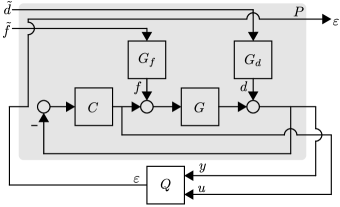
Figure 2: Closed-loop controlled regulator problem in generalized plant form, c.f., Figure 1. The generalized plant is highlighted ( ).

Consider the closed-loop control configuration in Figure 2, with single-input single-output plant $G(s)=\frac{(s+25)(s+15)(s+5)}{(s+40)(s+10)(s+3)}$ and controller $C(s)=15s+25$. The system is subjected to disturbances $d$ and actuator faults $f$, which are weighted by $G_{d}(s)$ and $G_{f}(s)$, respectively. Consider $\tilde{w}:=\begin{bmatrix}\tilde{d}&\tilde{f}\end{bmatrix}^{\top}$, $\tilde{z}:=\varepsilon$, $\tilde{y}:=\begin{bmatrix}y&u\end{bmatrix}^{\top}$, and $\tilde{u}:=\varepsilon$. The transfer function matrix of the generalized plant from $\begin{bmatrix}\tilde{w}&\tilde{u}\end{bmatrix}^{\top}$ to $\begin{bmatrix}\tilde{z}&\tilde{y}\end{bmatrix}^{\top}$, see Figure 2, is given by

$$\begin{bmatrix}\tilde{z}\\ \hline\cr\tilde{y}\end{bmatrix}=\left[\begin{array}[]{cc|l}0&0&I\\ \hline\cr S_{O}G_{d}&S_{O}G_{u}G_{f}&0\\ -S_{I}CG_{d}&-S_{I}CG_{u}G_{f}&0\end{array}\right]\begin{bmatrix}\tilde{w}\\ \hline\cr\tilde{u}\end{bmatrix},$$ (24)

where the input sensitivity $S_{I}=(I+CG)^{-1}$, and the output sensitivity $S_{O}=(I+GC)^{-1}$. The generalized disturbance input is split into $\tilde{w}=\begin{bmatrix}\tilde{w}_{\infty}&\tilde{w}_{-}\end{bmatrix}^{\top}=\begin{bmatrix}\tilde{d}&\tilde{f}\end{bmatrix}^{\top}$. It is aimed to impose $\mathcal{H}_{\infty}$ performance from $\tilde{w}_{\infty}$ to $\tilde{z}$ and impose $\mathcal{H}_{-}$ sensitivity from $\tilde{w}_{-}$ to $\tilde{z}$. Two arbitrary weighting filters are chosen to emphasize the shaping capability of the proposed method. To that end $G_{d}=\frac{s^{4}+62.8s^{3}+1392s^{2}+1.43\cdot{10}^{4}s+4.87\cdot{10}^{4}}{s^{4}+332s^{3}+2724s^{2}+8.10\cdot{10}^{4}s+1.22\cdot{10}^{5}}$ and $G_{f}=\frac{0.92s^{4}+43.25s^{3}+1911s^{2}+5976s+1.75\cdot{10}^{4}}{s^{4}+13.19s^{3}+3966s^{2}+2605s+3.90\cdot{10}^{4}}$.

Consider the multiobjective optimization problem, described by 23, where $\gamma_{0}=1$, $T=\mathcal{F}_{l}(P,Q)=\begin{bmatrix}T_{\tilde{z}\tilde{w}_{\infty}}&T_{\tilde{z}\tilde{w}_{-}}\end{bmatrix}^{\top}=\begin{bmatrix}T_{\varepsilon\tilde{d}}&T_{\varepsilon\tilde{f}}\end{bmatrix}^{\top}$, and the transfer matrices $T_{\tilde{z}\tilde{w}_{\infty}}$ and $T_{\tilde{z}\tilde{w}_{-}}$ admit the realization, described in Section 3.3, and are used to impose the maximum and minimum gain constraint, respectively.

Solving this problem with the synthesis method, described in Section 4.4, yields the optimum $\nu=0.76$. So the ratio $\mathcal{J}=\frac{\nu}{\gamma}=0.76$ and the obtained residual generator $Q$ is depicted in Figure 3. Hence, with this particular residual generator it is guaranteed that there is disturbance suppression $\left\lVert T_{\varepsilon\tilde{d}}\right\rVert_{\infty}<1$ and fault sensitivity $\left\lVert T_{\varepsilon\tilde{f}}\right\rVert_{-}>0.76$, see Figure 4. Additionally, the channels $T_{\varepsilon d}$ and $T_{\varepsilon f}$ are depicted with their found bounds $\gamma G_{d}^{-1}$ and $\nu G_{f}^{-1}$.

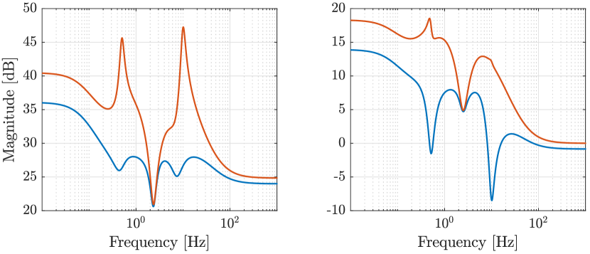
Figure 3: Residual filter $Q:\begin{bmatrix}y&u\end{bmatrix}^{\top}\rightarrow\varepsilon$ with optimal ratio $\mathcal{J}$ ( ). The updated filter $Q_{2}$, with the same $\mathcal{J}$, is shown as ( ).

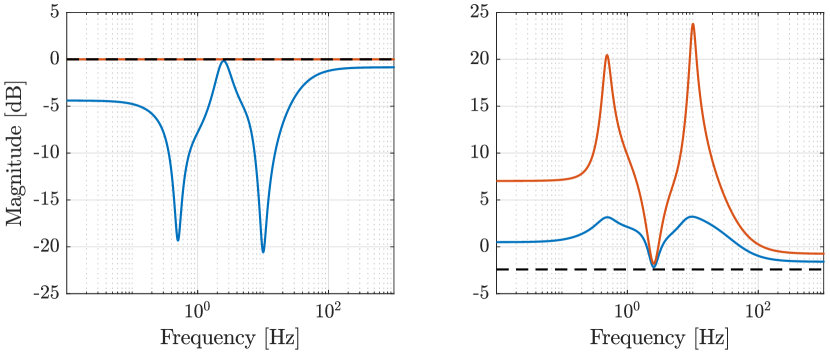
Figure 4: Closed-loop system, i.e., $T:\begin{bmatrix}\tilde{w}_{\infty}&\tilde{w}_{-}\end{bmatrix}^{\top}\rightarrow\varepsilon$, depicted as ( ). The obtained bounds $\gamma$ and $\nu$ are indicated as ( ), showing tight bounds near $\omega=2.5$ Hz. In this region, the fault to disturbance ratio is close to $\mathcal{J}$, whereas at other frequencies, fault sensitivity to disturbance attenuation ratio is higher. The closed-loop system with $Q_{2}$ is shown as ( ).

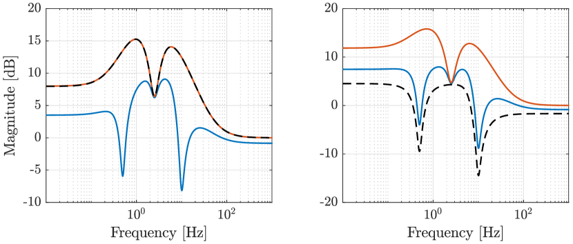
Figure 5: Closed-loop system without weighting filters, i.e., $T_{\varepsilon d}$ and $T_{\varepsilon f}$, depicted as ( ). The obtained bounds $\gamma G_{d}^{-1}$ and $\nu G_{f}^{-1}$ are depicted as ( ). Indeed, a filter $Q$ is found that satisfies the shaped upperbound and lowerbound. The closed-loop system with $Q_{2}$ is shown as ( ).

From Figure 4 and Figure 5 can be concluded that there is still margin to improve the fault sensitivity while simultaneously satisfying $\left\lVert T_{\varepsilon\tilde{d}}\right\rVert_{\infty}<1$. Updating the filter $Q$ with this difference, i.e. $Q_{2}=\tfrac{\gamma G_{d}^{-1}}{T_{\varepsilon d}}Q_{1}$, yields equivalent results to Liu and Zhou (2007). Note that the objective $\mathcal{J}=0.76$ remains equal.

6 Conclusion

In this paper, a new method to solve the $\mathcal{H}_{-}/\mathcal{H}_{\infty}$ problem is presented. In particular, a method is proposed to shape the minimum and maximum singular value of the closed-loop performance channel and its effectiveness is illustrated in the context of fault diagnosis. A bilinear matrix inequality is derived which can directly be implemented in combination with various multiobjective matrix inequalities and applied to synthesize filters for a wide range of control and estimation problems.

7 Acknowledgements

This work is supported by Topconsortia voor Kennis en Innovatie (TKI), and is supported by ASML Research, Veldhoven, The Netherlands.

8 APPENDIX: Synthesis Inequalities

The entries of the maximum gain synthesis LMI are

$$M_{11} =A{\color[rgb]{0,0,0}Y_{1}}+{\color[rgb]{0,0,0}Y_{1}}A^{\top}+B_{2}{\color[rgb]{0,0,0}C_{n}}+{\color[rgb]{0,0,0}C_{n}}^{\top}B_{2}^{\top},$$ (25a)

$$M_{12} =A+{\color[rgb]{0,0,0}A_{n}}^{\top}+B_{2}{\color[rgb]{0,0,0}D_{n}}C_{2},$$ (25b)

$$M_{13} =B_{1,j}+B_{2}{\color[rgb]{0,0,0}D_{n}}D_{21,j},$$ (25c)

$$M_{14} ={\color[rgb]{0,0,0}Y_{1}}C_{1,j}^{\top}+{\color[rgb]{0,0,0}C_{n}}^{\top}D_{12,j}^{\top},$$ (25d)

$$M_{22} ={\color[rgb]{0,0,0}X_{1}}A+A^{\top}{\color[rgb]{0,0,0}X_{1}}+{\color[rgb]{0,0,0}B_{n}}C_{2}+C_{2}^{\top}{\color[rgb]{0,0,0}B_{n}}^{\top},$$ (25e)

$$M_{23} ={\color[rgb]{0,0,0}X_{1}}B_{1,j}+{\color[rgb]{0,0,0}B_{n}}D_{21,j},$$ (25f)

$$M_{24} =C_{1,j}^{\top}+C_{2}^{\top}{\color[rgb]{0,0,0}D_{n}}^{\top}D_{12,j}^{\top},$$ (25g)

$$M_{33} =-{\color[rgb]{0,0,0}\gamma^{2}}I,$$ (25h)

$$M_{34} =D_{11,j}^{\top}+D_{21,j}^{\top}{\color[rgb]{0,0,0}D_{n}}^{\top}D_{12,j}^{\top},$$ (25i)

$$M_{44} =-I.$$ (25j)

The entries of the minimum gain synthesis BMI are

$$\begin{split}N_{11}&=A{\color[rgb]{0,0,0}Y_{1}}+B_{2}{\color[rgb]{0,0,0}C_{n}}+{\color[rgb]{0,0,0}Y_{1}}A^{\top}+{\color[rgb]{0,0,0}C_{n}}^{\top}B_{2}^{\top}\\ &\quad-\left({\color[rgb]{0,0,0}Y_{1}}C_{1,j}^{\top}+{\color[rgb]{0,0,0}C_{n}}^{\top}D_{12,j}^{\top}\right){\color[rgb]{0,0,0}\mathcal{Y}}\\ &\quad-{\color[rgb]{0,0,0}\mathcal{Y}}^{\top}\left(C_{1,j}{\color[rgb]{0,0,0}Y_{1}}+D_{12,j}{\color[rgb]{0,0,0}C_{n}}\right),\end{split}$$ (26a)

$$\begin{split}N_{12}&=A+{\color[rgb]{0,0,0}A_{n}}^{\top}+B_{2}{\color[rgb]{0,0,0}D_{n}}C_{2}\\ &\quad-\left({\color[rgb]{0,0,0}Y_{1}}C_{1,j}^{\top}+{\color[rgb]{0,0,0}C_{n}}^{\top}D_{12,j}^{\top}\right){\color[rgb]{0,0,0}\mathcal{Z}}\\ &\quad-{\color[rgb]{0,0,0}\mathcal{Y}}^{\top}\left(C_{1,j}+D_{12,j}{\color[rgb]{0,0,0}D_{n}}C_{2}\right),\end{split}$$ (26b)

$$\begin{split}N_{13}&=B_{1,j}+B_{2}{\color[rgb]{0,0,0}D_{n}}D_{21,j}\\ &\quad-{\color[rgb]{0,0,0}\mathcal{Y}}^{\top}\left(D_{11,j}+D_{12,j}{\color[rgb]{0,0,0}D_{n}}D_{21,j}\right)\\ &\quad-\left({\color[rgb]{0,0,0}Y_{1}}C_{1,j}^{\top}+{\color[rgb]{0,0,0}C_{n}}^{\top}D_{12,j}^{\top}\right){\color[rgb]{0,0,0}\mathcal{X}},\end{split}$$ (26c)

$$N_{14} ={\color[rgb]{0,0,0}\mathcal{Y}}^{\top},$$ (26d)

$$\begin{split}N_{22}&={\color[rgb]{0,0,0}X_{1}}A+{\color[rgb]{0,0,0}B_{n}}C_{2}+A^{\top}{\color[rgb]{0,0,0}X_{1}}+C_{2}^{\top}{\color[rgb]{0,0,0}B_{n}}^{\top}\\ &\quad-\left(C_{1,j}^{\top}+C_{2}^{\top}{\color[rgb]{0,0,0}D_{n}}^{\top}D_{12,j}^{\top}\right){\color[rgb]{0,0,0}\mathcal{Z}}\\ &\quad-{\color[rgb]{0,0,0}\mathcal{Z}}^{\top}\left(C_{1,j}+D_{12,j}{\color[rgb]{0,0,0}D_{n}}C_{2}\right),\end{split}$$ (26e)

$$\begin{split}N_{23}&={\color[rgb]{0,0,0}X_{1}}B_{1,j}+{\color[rgb]{0,0,0}B_{n}}D_{21,j}\\ &\quad-{\color[rgb]{0,0,0}\mathcal{Z}}^{\top}\left(D_{11,j}+D_{12,j}{\color[rgb]{0,0,0}D_{n}}D_{21,j}\right)\\ &\quad-\left(C_{1,j}^{\top}+C_{2}^{\top}{\color[rgb]{0,0,0}D_{n}}^{\top}D_{12,j}^{\top}\right){\color[rgb]{0,0,0}\mathcal{X}},\end{split}$$ (26f)

$$N_{24} ={\color[rgb]{0,0,0}\mathcal{Z}}^{\top},$$ (26g)

$$N_{33} ={\color[rgb]{0,0,0}\nu^{2}}I-{\color[rgb]{0,0,0}\mathcal{X}}^{\top}\left(D_{11}+D_{12}{\color[rgb]{0,0,0}D_{n}}D_{21}\right)$$ (26h)

$$\quad-\left(D_{11,j}^{\top}+D_{21,j}^{\top}{\color[rgb]{0,0,0}D_{n}}^{\top}D_{12,j}^{\top}\right){\color[rgb]{0,0,0}\mathcal{X}},$$ (26i)

$$N_{34} ={\color[rgb]{0,0,0}\mathcal{X}}^{\top},$$ (26j)

$$N_{44} =-I.$$ (26k)

References

• (1) ApS, MOSEK. (2023). MOSEK Optimization Toolbox for MATLAB.
• Bridgeman and Forbes (2015) Bridgeman, L.J. and Forbes, J.R. (2015). The minimum gain lemma. International Journal of Robust and Nonlinear Control, 25(14), 2515–2531.
• Caverly (2018) Caverly, R.J. (2018). Optimal Output Modification and Robust Control Using Minimum Gain and the Large Gain Theorem. Ph.D. thesis, University of Michigan, Michigan.
• Caverly and Forbes (2018) Caverly, R.J. and Forbes, J.R. (2018). $H_{\infty}$-Optimal Parallel Feedforward Control Using Minimum Gain. IEEE Control Systems Letters, 2(4), 677–682.
• Ding et al. (2000) Ding, S.X., Jeinsch, T., Frank, P.M., and Ding, E.L. (2000). A unified approach to the optimization of fault detection systems. International Journal of Adaptive Control and Signal Processing, 14(7).
• Gahinet and Apkarian (1994) Gahinet, P. and Apkarian, P. (1994). A linear matrix inequality approach to $H_{\infty}$ control. Int. J. Robust Nonlinear Control, 4(4), 421–448.
• Hassibi et al. (1999) Hassibi, A., How, J., and Boyd, S. (1999). A path-following method for solving BMI problems in control. In Proceedings of the 1999 American Control Conference, 1385–1389. IEEE, San Diego, CA, USA.
• Henry (2021) Henry, D. (2021). Theories for design and analysis of robust $H_{\infty}/H_{-}$ fault detectors. J. Franklin Inst., 358(1), 1152–1183.
• Hou and Patton (1996) Hou, M. and Patton, R. (1996). An LMI approach to $H_{-}/H_{\infty}$ fault detection observers. In UKACC International Conference on Control ’96 (Conf. Publ. No. 427), volume 1, 305–310 vol.1..
• Liu and Zhou (2007) Liu, N. and Zhou, K. (2007). Optimal solutions to multi-objective robust fault detection problems. In 2007 46th IEEE Conference on Decision and Control, 981–988.
• Lofberg (2004) Lofberg, J. (2004). YALMIP : A toolbox for modeling and optimization in MATLAB. In 2004 IEEE International Conference on Robotics and Automation, 284–289.
• Sadrnia et al. (1997) Sadrnia, M.A., Patton, R.J., and Chen, J. (1997). Robust $H_{\infty}/\mu$ fault diagnosis observer design. In 1997 European Control Conference (ECC), 1502–1507.
• Scherer et al. (1997) Scherer, C., Gahinet, P., and Chilali, M. (1997). Multiobjective output-feedback control via LMI optimization. IEEE Transactions on Automatic Control, 42(7), 896–911.
• Scherer and Weiland (2020) Scherer, C. and Weiland, S. (2020). Linear Matrix Inequalities in Control.
• Skogestad and Postlethwaite (2001) Skogestad, S. and Postlethwaite, I. (2001). Multivariable Feedback Control Analysis and Design. John Wiley & Sons, second edition edition.
• Stoustrup and H. Niemann (2002) Stoustrup, J. and H. Niemann, H. (2002). Fault estimation - a standard problem approach. Int. J. Robust Nonlinear Control, 12(8), 649–673.
• Wang et al. (2007) Wang, J.L., Yang, G.H., and Liu, J. (2007). An LMI approach to $H_{-}$ index and mixed $H_{-}/H_{\infty}$ fault detection observer design. Automatica, 43(9), 1656–1665.
• Zhong et al. (2003) Zhong, M., Ding, S.X., Lam, J., and Wang, H. (2003). An LMI approach to design robust fault detection filter for uncertain LTI systems. Automatica, 8.