Entropy-split multidimensional summation-by-parts discretization of the Euler and compressible Navier-Stokes equations

Abstract

High-order Hadamard-form entropy stable multidimensional summation-by-parts discretizations of the Euler and compressible Navier-Stokes equations are considerably more expensive than the standard divergence-form discretization. In search of a more efficient entropy stable scheme, we extend the entropy-split method for implementation on unstructured grids and investigate its properties. The main ingredients of the scheme are Harten’s entropy functions, diagonal-$\mathsf{E}$ summation-by-parts operators with diagonal norm matrix, and entropy conservative simultaneous approximation terms (SATs). We show that the scheme is high-order accurate and entropy conservative on periodic curvilinear unstructured grids for the Euler equations. An entropy stable matrix-type interface dissipation operator is constructed, which can be added to the SATs to obtain an entropy stable semi-discretization. Fully-discrete entropy conservation is achieved using a relaxation Runge-Kutta method. Entropy stable viscous SATs, applicable to both the Hadamard-form and entropy-split schemes, are developed for the compressible Navier-Stokes equations. In the absence of heat fluxes, the entropy-split scheme is entropy stable for the compressible Navier-Stokes equations. Local conservation in the vicinity of discontinuities is enforced using an entropy stable hybrid scheme. Several numerical problems involving both smooth and discontinuous solutions are investigated to support the theoretical results. Computational cost comparison studies suggest that the entropy-split scheme offers substantial efficiency benefits relative to Hadamard-form multidimensional SBP-SAT discretizations.

1 Introduction

In recent years, research interest in nonlinearly stable skew-symmetric discretizations of the governing equations of fluid dynamics has been revived [1, 2, 3, 4, 5]. These studies are partly driven by the desire to improve upon some of the theoretical and practical aspects of the high-order Hadamard-form or two-point flux entropy conservative or dissipative scheme [6, 7, 8, 9, 10, 11]. Despite its demonstrated robustness [12, 13, 14, 15, 16, 17], the Hadamard-form entropy conservative scheme is so far incomplete as there are remaining pieces that are actively being researched such as positivity preservation of thermodynamic quantities [18, 19] and entropy stable boundary conditions [20, 21, 22, 23, 15]. The efficiency of the scheme has also been given due attention [24, 25], as its computational cost is larger than that of the divergence-form implementation. Nonlinearly stable skew-symmetric split schemes may potentially allow bypassing some of these issues although at a cost of compromising other coveted properties such as mass conservation, kinetic energy preservation, and robustness. The entropy-split method is an example of nonlinearly stable skew-symmetric schemes, which has been applied in the traditional finite difference fashion [26, 27, 1, 2]. Entropy splitting refers to a skew-symmetric splitting of the flux derivatives of the Euler equations into conservative and nonconservative portions using the symmetrizability and homogeneity properties of the equations [27]. So far, the entropy-split method has not been generalized for discontinuous element-type implementations, which approximate the solution on a mesh consisting of non-overlapping elements supporting solution discontinuities at element interfaces. The principal objective of this paper is to extend the existing skew-symmetric entropy-split scheme to element-type implementations and shed light on the trade-offs between a few of the numerical properties afforded by it in comparison to the Hadamard-form implementation of the Euler and compressible Navier-Stokes equations on unstructured meshes. In particular, the study aims to provide some insights to the following questions: how robust is the entropy-split method compared to the Hadamard-form scheme? how much more efficient is it? how can its loss of conservation be mitigated?

In his seminal paper of 1983, Harten [28] proposed a family of entropy functions that symmetrizes the Euler and compressible Navier-Stokes equations without the heat fluxes. Furthermore, he showed that the fluxes in the Euler equations are homogeneous in the entropy variables corresponding to the proposed entropy functions. Olsson and Oliger [29] used these symmetry and homogeneity results to write the Euler equations in a skew-symmetric entropy-split form and obtained a nonlinear energy estimate under some assumptions. Subsequently, Gerittsen and Olsson [26] designed a split high-order entropy-conserving scheme by discretizing the entropy-split form of the Euler equations using the classical summation-by-parts (SBP) finite difference operators of Strand [30]. Yee et al. [27] investigated various aspects of the entropy-split scheme including the choice of the arbitrary splitting parameter, effects of the splitting on nonlinear stability, and application of characteristic-based filters. Later, Svärd and Mishra [31] constructed entropy stable boundary conditions which extend the entropy stability of the entropy-split scheme to bounded domains. More recently, Sjögreen and Yee [1] showed that the entropy-split scheme is entropy conservative for the Euler equations and demonstrated its robustness in a series of papers [3, 2, 32]. For a more detailed review and recent developments of the entropy-split scheme, see [2] and the references therein.

In this paper, we extend the entropy-split scheme to element-type implementations, which facilitate flexible mesh generation around complex geometries, especially when applied with simplicial elements. The main ingredients of the new scheme are Harten’s entropy functions, diagonal-norm SBP operators [33, 9] with collocated volume and surface nodes, and entropy conservative or dissipative simultaneous approximation terms (SATs) [34], which are coupling terms at element interfaces and boundaries. We show that the scheme is high-order accurate and entropy conservative on periodic general curvilinear unstructured grids for the Euler equations. Generalization of the scheme to bounded domains is not pursued in this article, but it is possible to make this extension using the entropy stable boundary conditions proposed by Svärd and Mishra [31]. If heat fluxes are neglected, then the entropy stability result also applies to the compressible Navier-Stokes equations provided that appropriate viscous SATs are used. To this end, we extend the viscous SATs developed in [35, 36] to systems of equations with a positive semidefinite diffusivity tensor, alleviating the requirement to have a positive definite diffusivity tensor for stability. These viscous SATs are applicable to the entopy-split as well as Hadamard-form discretizations and do not require setting the viscous terms as a system of first-order equations unlike the widely used viscous SATs in the literature [8, 11, 37, 38, 15].

The entropy-split discretization is not conservative in the sense of Lax-Wendroff [39]. Hence, for problems with discontinuous solutions, we introduce a strategy to mitigate the effects of the loss of conservation such as incorrect shock speed. The main idea is to enforce local conservation by using the Hadamard-form discretization near discontinuities while ensuring entropy stability via a seamless coupling between the Hadamard-form and entropy-split schemes. This strategy allows one to benefit from the conservative property of the Hadamard-form discretization in critical areas of the computational domain and the efficiency of the entropy-split scheme elsewhere without compromising entropy stability. A similar strategy of switching between different schemes, but without enforcing entropy stability, has been proposed by other authors, e.g., see [40, 3]. Hou and LeFloch [40] showed that such a strategy of enforcing local conservation guarantees convergence to the weak solution for scalar conservation laws.

High-order dissipation operators have been designed [41, 42, 43] to augment the Hadamard-form entropy conservative scheme with the physical property needed at shock waves. The dissipation operators are usually integrated with the inviscid SATs, producing an entropy dissipative variant of the entropy conservative scheme. In this work, we design a matrix-type interface dissipation operator for the entropy-split and Sjögreen-Yee Hadamard-form [1] discretizations. Finally, the extension from semi-discrete to full entropy conservation or dissipation is achieved by using the fourth-order explicit relaxation Runge-Kutta (RRK4) method of Ranocha et al. [44]. Several benchmark problems involving both smooth and discontinuous solutions are investigated to support our theoretical findings and compare various numerical properties of the entropy-split and Hadamard-form discretizations. We also present efficiency comparisons between these two types of discretizations as applied to problems governed by the Euler and compressible Navier-Stokes equations.

In the next section, we begin by introducing SBP operators and the notation used, followed by a review of the homogeneity and symmetrization of the Euler and compressible Navier-Stokes equations. In Section 3, we present the continuous entropy conservation and stability analysis. Section 4 contains the discrete entropy conservation analysis for the Euler equations, the conservation error analysis of the entropy-split scheme, a strategy to handle discontinuous solutions, and the construction of interface dissipation operators. In Section 5, extension of the entropy-split scheme to the compressible Navier-Stokes equations is discussed and some implementation details are presented in Section 6. Numerical results are presented in Section 7 followed by conclusions in Section 8.

2 Preliminaries

2.1 SBP operators and notation

Spatial discretizations are handled using element-type SBP operators, which play a crucial role in the entropy stability analysis. The spatial domain, $\Omega$, is assumed to be compact and connected, and it is tessellated into $n_{e}$ non-overlapping elements, ${\mathcal{T}}_{h}\coloneqq\{\{\Omega_{k}\}_{k=1}^{n_{e}}:\Omega=\cup_{k=1}^{n_{e}}{\Omega}_{k}\}$. The boundaries of each element are assumed to be piecewise smooth and will be referred to as facets or interfaces, and the union of the facets of element $\Omega_{k}$ is denoted by $\Gamma_{k}\coloneqq\partial\Omega_{k}$. The set of all interior interfaces is denoted by $\Gamma^{I}\coloneqq\{\Gamma_{k}\cap\Gamma_{v}:k,v=1,\dots,n_{e},k\neq v\}$. The set of facets of $\Omega_{k}$ that are also interior facets is denoted by $\Gamma^{I}_{k}\coloneqq\Gamma^{I}\cap\Gamma_{k}$, and $\Gamma\coloneqq\{\partial\Omega\cap\Gamma_{k}:k=1,\dots,n_{e}\}$ delineates the set of all boundary facets. The set of $n_{p}$ volume nodes in element $\Omega_{k}$ is represented by $S_{k}=\{\bm{x}_{j}\}_{j=1}^{n_{p}}$, and $n_{f}$ denotes the number of nodes on facet $\gamma\in\Gamma_{k}$. Scalar functions are written in uppercase script type, e.g., $\mathcal{U}_{k}\in\mathcal{C}^{\infty}({\Omega}_{k})$, and vector-valued functions of dimension $n$ are represented by boldface uppercase script letters, e.g., $\bm{\mathcal{W}}_{k}\in[L^{2}({\Omega}_{k})]^{n}$. The space of polynomials of total degree $p$ is denoted by $\mathbb{P}^{p}({\Omega}_{k})$. Vectors containing function values at a set of grid points are denoted by bold letters, e.g., $\bm{{u}}_{k}\in\mathbb{R}^{n_{p}}$. We define $h\coloneqq\max_{a,b\in S_{k}}\left|\left|a-b\right|\right|_{2}$ as the nominal element size. Matrices are denoted by sans-serif uppercase letters, e.g., $\mathsf{V}\in\mathbb{R}^{{n_{p}}\times{n_{p}}}$; $\bm{1}$ denotes a vector consisting of all ones, $\bm{0}$ denotes a vector or matrix consisting of all zeros. The sizes of $\bm{1}$ and $\bm{0}$ should be clear from context. Finally, $\mathsf{I}_{n}$ represents the identity matrix of size $n\times n$.

SBP operators on a physical element, $\Omega_{k}$, are defined as follows [33].

Definition 1.

The matrix ${\mathsf{D}}_{\bm{x}_{i}k}\in\mathbb{R}^{{n_{p}}\times{n_{p}}}$ is a degree $p$ SBP operator in the $i$-direction approximating the first derivative $\partialderivative{\bm{x}_{i}}$ on the set of nodes ${S}_{k}=\{\bm{x}_{j}\}_{j=1}^{n_{p}}$ if

1. $[{\mathsf{D}}_{\bm{x}_{i}k}\bm{p}]_{j}={\partialderivative{\mathcal{P}}{{x}_{i}}}({\bm{x}_{j}})$ for all $\mathcal{P}\in\mathbb{P}^{p}({\Omega}_{k})$

2. ${\mathsf{D}}_{\bm{x}_{i}k}={\mathsf{H}}^{-1}_{k}{\mathsf{Q}}_{\bm{x}_{i}k}$ where ${\mathsf{H}}_{k}$ is a symmetric positive definite (SPD) matrix, and

3. ${\mathsf{Q}}_{\bm{x}_{i}k}={\mathsf{S}}_{\bm{x}_{i}k}+\frac{1}{2}{\mathsf{E}}_{\bm{x}_{i}k}$ where ${\mathsf{S}}_{\bm{x}_{i}k}=-{\mathsf{S}}_{\bm{x}_{i}k}^{T}$, ${\mathsf{E}}_{\bm{x}_{i}k}={\mathsf{E}}_{\bm{x}_{i}k}^{T}$ and ${\mathsf{E}}_{\bm{x}_{i}k}$ satisfies

   $$\bm{p}^{T}{\mathsf{E}}_{\bm{x}_{i}k}\bm{q}=\int_{{\Gamma}_{k}}\mathcal{P}\mathcal{Q}\;{n}_{{x}_{i}}\differential{\Gamma}$$

   $\forall\mathcal{P},\mathcal{Q}\in\mathbb{P}^{r}({\Omega}_{k})$, where $r\geq p$, and ${n}_{{x}_{i}}$ is the $i$-component of the outward pointing unit normal vector on ${\Gamma}_{k}$.

The third property in Definition 1 implies that $\mathsf{Q}_{{x}_{i}k}+\mathsf{Q}_{{x}_{i}k}^{T}=\mathsf{E}_{{x}_{i}k}$, which is referred to as the SBP property. The SBP operators in Definition 1 contain grid metric terms as they are defined for the physical element $\Omega_{k}$, which may be curved. We make the following assumption regarding the geometric mapping from the reference to physical elements.

Assumption 1.

We assume that there is a bijective and time-independent polynomial mapping of degree $p_{\text{geom}}$ from the reference to the physical elements. Furthermore, we assume that the degree of the mapping is limited to $p_{\text{geom}}\leq p+1$ and $p_{\text{geom}}\leq\lfloor p/2\rfloor+1$ in two and three dimensions, respectively, where $p$ is the degree of the SBP operator.

Assumption 1 ensures that the discrete metric identities are satisfied on curved elements [10, 45]. If a higher degree polynomial mapping is needed to represent a three-dimensional geometry, then one may employ the strategy outlined in [10], which involves solving elementwise quadratic optimization problems. For construction of multidimensional SBP operators, we refer the reader to [33, 46, 9], and see, e.g., [10, 45, 36] for their implementation on curved elements. A more general review of SBP-SAT discretizations can be found in [47, 48].

In this work, we exclusively consider SBP operators with diagonal $\mathsf{H}$ and $\mathsf{E}$ matrices. In the one-dimensional case, we use the Legendre-Gauss-Lobatto (LGL) operators [49, 50, 8, 51] and higher-dimensional cases use the SBP diagonal-$\mathsf{E}$ multidimensional operators [9, 33]. The diagonal of the norm matrix, $\mathsf{H}$, contains strictly positive entries which are weights of a quadrature rule of at least degree $2p-1$. Hence, it approximate an inner product,

$$\bm{p}_{k}^{T}\mathsf{H}_{k}\bm{q}_{k}=\int_{\Omega_{k}}\mathcal{P}\mathcal{Q}\differential{\Omega},\quad\forall\;\mathcal{P}\mathcal{Q}\in\mathbb{P}^{r}({\Omega}_{k}),\quad r\leq 2p-1,$$ (1)

and is used to define the $\mathsf{H}$-norm, $\left|\left|\bm{u}\right|\right|_{\mathsf{H}}^{2}=\bm{u}^{T}\mathsf{H}\bm{u}$. The facet nodes of diagonal-$\mathsf{E}$ SBP operators are collocated with the volume nodes. This implies that an extrapolation operator, $\mathsf{R}_{\gamma k}\in\mathbb{R}^{{n_{f}}\times{n_{p}}}$, that extrapolates the solution at the volume nodes to the facet nodes will simply produce the solution values at the facet nodes. Assuming that a quadrature rule of degree at least $2p$ with strictly positive weights exists on the nodes of facet $\gamma\in\Gamma_{k}$ with its weights contained in the diagonal matrix $\mathsf{B}_{\gamma}\in\mathbb{R}^{{n_{f}}\times{n_{f}}}$, the matrix ${\mathsf{E}}_{\bm{x}_{i}k}$ can be decomposed as [46]

$${\mathsf{E}}_{\bm{x}_{i}k}=\sum_{\gamma\in\Gamma_{k}}{\mathsf{E}}_{\bm{x}_{i}}^{kk},\quad\text{where}\;\;{\mathsf{E}}_{\bm{x}_{i}}^{kk}=\mathsf{R}_{\gamma k}^{T}\mathsf{B}_{\gamma}{\mathsf{N}}_{\bm{x}_{i}\gamma}\mathsf{R}_{\gamma k},$$ (2)

where ${\mathsf{N}}_{\bm{x}_{i}\gamma}\in\mathbb{R}^{{n_{f}}\times{n_{f}}}$ is a diagonal matrix containing the $i$-component of the outward unit normal vector on facet $\gamma$. The facet nodes on adjoining facets of $\Omega_{k}$ and its neighboring element, $\Omega_{v}$, coincide, i.e., only conforming meshes are considered. The coupling terms between $\Omega_{k}$ and $\Omega_{v}$ make use of the following matrices and their relation,

$${\mathsf{E}}_{\bm{x}_{i}}^{kv}=\mathsf{R}_{\gamma k}^{T}\mathsf{B}_{\gamma}{\mathsf{N}}_{\bm{x}_{i}\gamma}\mathsf{R}_{\gamma v}, {\mathsf{E}}_{\bm{x}_{i}}^{vk}=-\mathsf{R}_{\gamma v}^{T}\mathsf{B}_{\gamma}{\mathsf{N}}_{\bm{x}_{i}\gamma}\mathsf{R}_{\gamma k}, {\mathsf{E}}_{\bm{x}_{i}}^{kv}=-({\mathsf{E}}_{\bm{x}_{i}}^{vk})^{T}.$$ (3)

For systems of equations with $n_{c}$ components, the operators defined so far are applied using a Kronecker product with the identity matrix, e.g., $\overline{\mathsf{D}}_{\bm{x}_{i}k}={\mathsf{D}}_{\bm{x}_{i}k}\otimes\mathsf{I}_{n_{c}}$, where the overbar indicates application to systems of equations.

2.2 Governing equations

The $d$-dimensional compressible Navier-Stokes equations can be written as,

$$\dfrac{\partial\bm{\mathcal{U}}}{\partial t}+\sum_{i=1}^{d}\dfrac{\partial}{\partial{x}_{i}}\bm{\mathcal{F}}^{I(i)} =\sum_{i=1}^{d}\dfrac{\partial}{\partial{x}_{i}}\bm{\mathcal{F}}^{V(i)},\quad\bm{x}=[{\color[rgb]{0,0,0}x_{1},x_{2},x_{3}}]^{T}\in\Omega,\quad t\in[0,t_{f}],$$ (4)

$$\mathcal{B}\bm{\mathcal{U}}\left(\bm{x},t\right) =\bm{\mathcal{U}}_{\Gamma},\quad\bm{x}\in\Gamma,$$

$$\bm{\mathcal{U}}\left(\bm{x},0\right) =\bm{\mathcal{U}}_{0},\quad\bm{x}\in\Omega{\color[rgb]{0,0,0},}$$

where $\mathcal{U}(\bm{x},t)$ contains the conservative variables, $\bm{\mathcal{F}}^{I(i)}(\bm{\mathcal{U}})$ and $\bm{\mathcal{F}}^{V(i)}(\mathcal{U},\frac{\partial\bm{\mathcal{U}}}{\partial\bm{x}_{j}})$ are the inviscid (Euler) and viscous fluxes in the $i$-direction, respectively, and $\mathcal{B}$ is a boundary operator. The Euler equations are obtained by nullifying the right-hand side (RHS) of the first line in 4. Assuming a Newtonian fluid, the conservative variables, the inviscid, and the viscous fluxes in three dimensions are given by

$$\bm{\mathcal{U}}=\begin{bmatrix}\rho\\ \rho{\color[rgb]{0,0,0}V_{1}}\\ \rho{\color[rgb]{0,0,0}V_{2}}\\ \rho{\color[rgb]{0,0,0}V_{3}}\\ e\end{bmatrix},\;\;\bm{\mathcal{F}}^{I(i)}=\begin{bmatrix}\rho V_{i}\\ \rho V_{i}V_{1}+\delta_{i1}p\\ \rho V_{i}V_{2}+\delta_{i2}p\\ \rho V_{i}V_{3}+\delta_{i3}p\\ (e+p)V_{i}\end{bmatrix},\;\;\bm{\mathcal{F}}^{V(i)} =\begin{bmatrix}0\\ \tau_{{x}_{i}{\color[rgb]{0,0,0}x_{1}}}\\ \tau_{{x}_{i}{\color[rgb]{0,0,0}x_{2}}}\\ \tau_{{x}_{i}{\color[rgb]{0,0,0}x_{3}}}\\ \Sigma_{j=1}^{d}V_{j}\tau_{{x}_{i}{x}_{j}}\end{bmatrix}+\begin{bmatrix}0\\ 0\\ 0\\ 0\\ \kappa\frac{\partial T}{\partial{x}_{i}}\end{bmatrix},\;\;\tau_{{x}_{i}{x}_{j}}=\mu\left(\dfrac{\partial V_{i}}{\partial{x}_{j}}+\dfrac{\partial V_{j}}{\partial{x}_{i}}-\frac{2}{3}\delta_{ij}\sum_{k=1}^{d}\dfrac{\partial V_{k}}{\partial{x}_{k}}\right){\color[rgb]{0,0,0},}$$ (5)

where $\rho$ is the density, ${\color[rgb]{0,0,0}\bm{V}=[V_{1},V_{2},V_{3}]^{T}}$ contains the $\bm{x}=[{\color[rgb]{0,0,0}x_{1},x_{2},x_{3}}]^{T}$ velocity components, $p$ is the pressure, $e$ is the total energy, $T$ is the temperature, $\mu$ is the dynamic viscosity, $\kappa$ is the heat conductivity, and $\delta_{ij}$ is the Kronecker delta. Assuming thermally and calorically perfect gases, the system is closed by the relation $e={p}/{(\gamma-1)}+{\rho}\bm{V}^{T}\bm{V}/2$, where $\gamma=7/5$ is the ratio of specific heats. The viscous fluxes are written as a sum of the viscous and heat fluxes, which is a suitable form for later discussion.

2.3 Homogeneity

Definition 2.

$\bm{\mathcal{F}}\left(\bm{\mathcal{U}},\bm{\mathcal{V}}\right)$ is a degree $n$ homogeneous function in the argument $\bm{\mathcal{U}}$ if $\bm{\mathcal{F}}\left(\eta\bm{\mathcal{U}},\bm{\mathcal{V}}\right)=\eta^{n}\bm{\mathcal{F}}\left(\bm{\mathcal{U}},\bm{\mathcal{V}}\right)$, $\eta\neq 0$.

The definition of homogeneous functions can be found in several books, e.g., [52], and the following lemma is a restatement of Euler’s homogeneous function theorem, e.g., see [53], in suitable forms for later use. The proof of the lemma is omitted as it follows from elementary application of calculus and Definition 2.

Lemma 1.

Consider a function, $\bm{\mathcal{F}}=\bm{\mathcal{F}}\left(\bm{\mathcal{U}},\bm{\mathcal{V}}\right)$, that is degree $n$ homogeneous in its first argument, and let $\mathsf{A}=\frac{\partial\bm{\mathcal{F}}}{\partial\bm{\mathcal{U}}}$. Then, the the following identity holds,

$$\mathsf{A}\bm{\mathcal{U}} =n\bm{\mathcal{F}},$$ (6)

Furthermore, if $\bm{\mathcal{F}}=\bm{\mathcal{F}}\left(\bm{\mathcal{U}}\right)$, then, in addition to 6, it can be shown that

$$\dfrac{\partial}{\partial x}\left(\mathsf{A}\bm{\mathcal{U}}\right) =n\dfrac{\partial\bm{\mathcal{F}}}{\partial x}=n\mathsf{A}\dfrac{\partial\bm{\mathcal{U}}}{\partial x},$$ (7)

or equivalently,

$$\frac{\partial\mathsf{A}}{\partial x}\bm{\mathcal{U}}=(n-1)\mathsf{A}\frac{\partial\bm{\mathcal{U}}}{\partial x}.$$ (8)

It is well known that the inviscid fluxes are homogeneous functions of degree one in the conservative variables, e.g., see [53]. Similarly, the viscous fluxes are homogeneous functions of degree one in the argument $\frac{\partial\bm{\mathcal{U}}}{\partial{x}_{j}}$ as well as $\frac{\partial\bm{\mathcal{Q}}}{\partial{x}_{j}}$, where $\bm{\mathcal{Q}}=[\rho,{\color[rgb]{0,0,0}V_{1},V_{2},V_{3}},T]^{T}$ is a vector of the primitive variables. It can also be shown that the viscous fluxes are homogeneous functions of degree $-1$ in the argument $\bm{\mathcal{U}}$ but not homogeneous in $\bm{\mathcal{Q}}$. Hence, Lemma 1 implies that

$$\bm{\mathcal{F}}^{I(i)} =\mathsf{A}_{i}\bm{\mathcal{U}}, \mathsf{A}_{i}\coloneqq\dfrac{\partial\bm{\mathcal{F}}^{I(i)}}{\partial\bm{\mathcal{U}}}, \dfrac{\partial\bm{\mathcal{F}}^{I(i)}}{\partial{x}_{i}}=\mathsf{A}_{i}\dfrac{\partial\bm{\mathcal{U}}}{\partial{x}_{i}},$$ (9)

$$\bm{\mathcal{F}}^{V(i)} =\sum_{j=1}^{d}\mathsf{K}_{ij}\dfrac{\partial\bm{\mathcal{U}}}{\partial x_{j}}=\sum_{j=1}^{d}\mathsf{C}_{ij}\dfrac{\partial\bm{\mathcal{Q}}}{\partial x_{j}}, \mathsf{K}_{ij}\coloneqq\dfrac{\partial\bm{\mathcal{F}}^{V(i)}}{\partial\left(\frac{\partial\bm{\mathcal{U}}}{\partial{x}_{j}}\right)}, \mathsf{C}_{ij}\coloneqq\dfrac{\partial\bm{\mathcal{F}}^{V(i)}}{\partial\left(\frac{\partial\bm{\mathcal{Q}}}{\partial{x}_{j}}\right)}.$$ (10)

The compressible Navier-Stokes equations, 4, can therefore be written as [54]

$$\dfrac{\partial\bm{\mathcal{U}}}{\partial t}+\sum_{i=1}^{d}\mathsf{A}_{i}\dfrac{\partial\bm{\mathcal{U}}}{\partial{x}_{i}}=\sum_{i=1}^{d}\dfrac{\partial}{\partial{x}_{i}}\left(\sum_{j=1}^{d}\mathsf{K}_{ij}\dfrac{\partial\bm{\mathcal{U}}}{\partial{x}_{j}}\right).$$ (11)

2.4 Symmetrization

A stability analysis via the energy method requires symmetrization of the inviscid flux Jacobians, $\mathsf{A}_{i}$, and the diffusivity tensor, i.e., the block matrix containing the viscous flux Jacobians, $\mathsf{K}=[\mathsf{K}_{ij}]$. One way to achieve this is through a change of variables. For hyperbolic systems, symmetrization of the flux Jacobians under a change of variables is intimately linked to the existence of an entropy function and the corresponding entropy fluxes; in fact, one implies the other [28]. However, not all entropy functions that symmetrize the inviscid flux Jacobians also symmetrize the diffusivity tensor. Entropy functions that enable symmetrization of both via a change of variables are referred to as generalized entropy functions [55].

The Euler equations are accompanied by a scalar entropy balance equation that describes the second law of thermodynamics; i.e., the physical entropy, $s=\ln(p\rho^{-\gamma})$, in a system does not decrease, or mathematically,

$$\dfrac{{\rm d}}{{\rm d}t}\int_{\Omega}\mathcal{S}\differential{\Omega}+\sum_{i=1}^{d}\int_{\Gamma}\mathcal{G}^{(i)}n_{\bm{x}_{i}}\differential{\Gamma}\leq 0,$$ (12)

where the mathematical entropy function and entropy flux are given, respectively, by

$$\mathcal{S} =-\rho\mathcal{H}(s)/(\gamma-1),$$ (13)

$$\mathcal{G}^{(i)} =V_{i}\mathcal{S},$$ (14)

and $\mathcal{H}$ is any differentiable function such that $\frac{\partial^{2}\mathcal{H}}{\partial\mathcal{S}^{2}}\big{/}\frac{\partial\mathcal{H}}{\partial\mathcal{S}}<1/\gamma$ [28]. Note that due to the negative scaling in the definition of $\mathcal{S}$, the inequality in 12 states that the mathematical entropy in a system does not increase. Furthermore, the inequality becomes an equality if the solution is smooth. The entropy inequality, 12, also applies to the compressible Navier-Stokes equations, but with some restrictions on $\mathcal{S}$. Hughes et al. [54] proved that the only family of generalized entropy functions for the compressible Navier-Stokes equations are those that are affine transformations of $s$, i.e., $\mathcal{H}(s)$ must be linear in $s$. Usually, the generalized entropy function

$$\mathcal{S}_{G}=-\rho s/(\gamma-1)$$ (15)

is used for the Hadamard-form entropy stable discretizations of the compressible Navier-Stokes equations. Entropy-split schemes, however, use a family of entropy functions that was introduced by Harten [28],

$$\mathcal{S}_{H}=-\frac{\gamma+\alpha}{\gamma-1}\rho\exp({\frac{s}{\alpha+\gamma}})=\beta\rho\left({p}{\rho^{-\gamma}}\right)^{\frac{1}{\alpha+\gamma}},$$ (16)

where $\beta=-(\gamma+\alpha)/(\gamma-1)$, and $\alpha$ is an arbitrary parameter satisfying the condition $\alpha>0$ or $\alpha<-\gamma$. It is possible to apply Harten’s entropy functions to construct an Hadamard-form discretization that is entropy conservative or stable for the Euler equations [1].

For the symmetrization of 11, we first introduce the entropy variables defined as

$$\bm{\mathcal{W}}^{T}\coloneqq\dfrac{\partial\mathcal{S}}{\partial\bm{\mathcal{U}}}.$$ (17)

Applying a change of variables, 11 can be rewritten as

$$\tilde{\mathsf{A}}_{0}\dfrac{\partial\bm{\mathcal{W}}}{\partial t}+\sum_{i=1}^{d}\tilde{\mathsf{A}}_{i}\dfrac{\partial\bm{\mathcal{W}}}{\partial{x}_{i}}=\sum_{i=1}^{d}\dfrac{\partial}{\partial{x}_{i}}\left(\sum_{j=1}^{d}\tilde{\mathsf{K}}_{ij}\dfrac{\partial\bm{\mathcal{W}}}{\partial{x}_{j}}\right),$$ (18)

where

$$\tilde{\mathsf{A}}_{0}=\frac{\partial\bm{\mathcal{U}}}{\partial\bm{\mathcal{W}}}, \quad\tilde{\mathsf{A}}_{i}=\mathsf{A}_{i}\tilde{\mathsf{A}}_{0}, \quad\tilde{\mathsf{K}}_{ij}=\mathsf{K}_{ij}\tilde{\mathsf{A}}_{0}.$$ (19)

If $\mathcal{S}=\mathcal{S}_{G}$, then $\tilde{\mathsf{A}}_{0}$, $\tilde{\mathsf{A}}_{i}$, and $\tilde{\mathsf{K}}=[\tilde{\mathsf{K}}_{ij}]$ will be symmetric simultaneously, and we have $\tilde{\mathsf{A}}_{0}\succ 0$ and $\tilde{\mathsf{K}}\succeq 0$, where $\succ$ and $\succeq$ denote symmetric positive definiteness and symmetric positive semidefiniteness, respectively. If, instead, $\mathcal{S}=\mathcal{S}_{H}$, then $\tilde{\mathsf{A}}_{0}\succ 0$ and $\tilde{\mathsf{A}}_{i}=\tilde{\mathsf{A}}_{i}^{T}$, but $\tilde{\mathsf{K}}\not\succeq 0$ unless the heat fluxes in the compressible Navier-Stokes equations are neglected. The positive definiteness of $\tilde{\mathsf{A}}_{0}$ implies that its inverse exists and that there is a bijective mapping between the conservative and entropy variables. Furthermore, the fact that $\tilde{\mathsf{A}}_{0}$ and $\tilde{\mathsf{A}}_{i}$ are symmetric implies that $\bm{\mathcal{U}}$ and $\bm{\mathcal{F}}^{I(i)}$ are Jacobians of scalar functions with respect to the entropy variables, i.e.,

$$\bm{\mathcal{U}}^{T}=\dfrac{\partial\varphi}{\partial\bm{\mathcal{W}}},$$ (20)

$$\left[\bm{\mathcal{F}}^{I(i)}\right]^{T}=\dfrac{\partial\psi^{(i)}}{\partial\bm{\mathcal{W}}},$$ (21)

where the scalar functions $\varphi$ and $\psi^{(i)}$ are called the potential and potential flux functions, respectively, and they satisfy the following identities [56, 57, 28],

$$\varphi =\bm{\mathcal{W}}^{T}\bm{\mathcal{U}}-\mathcal{S},$$ (22)

$$\psi^{(i)} =\bm{\mathcal{W}}^{T}\bm{\mathcal{F}}^{I(i)}-\mathcal{G}^{(i)}.$$ (23)

3 Continuous entropy stability analysis

Olsson and Oliger [29] proposed a splitting of the symmetrized Euler fluxes that allows one to exploit the homogeneity of the fluxes to show entropy conservation. At the heart of the splitting is Harten’s family of entropy functions, which, unlike the symmetrization using $\mathcal{S}_{G}$, transfers the homogeneity of the Euler equations to the symmetrized system. For smooth solutions, the entropy-split Euler equations are written as

$$\dfrac{\partial\bm{\mathcal{U}}}{\partial t}+\frac{\beta}{\beta+1}\sum_{i=1}^{d}\dfrac{\partial\bm{\mathcal{F}}^{I(i)}}{\partial{x}_{i}}+\frac{1}{\beta+1}\sum_{i=1}^{d}\tilde{\mathsf{A}}_{i}\dfrac{\partial\bm{\mathcal{W}}}{\partial{x}_{i}}=\bm{0},$$ (24)

where the relative amount of conservative and nonconservative portions of the splitting is controlled by the arbitrary parameter $\beta$, and the entropy variables are given by

$$\bm{\mathcal{W}}^{T}=\dfrac{\partial\mathcal{S}_{H}}{\partial\bm{\mathcal{U}}}=\frac{\rho}{p}(p\rho^{-\gamma})^{\frac{1}{\alpha+\gamma}}\left[\begin{array}[]{ccccc}-\frac{\alpha}{\gamma-1}\frac{p}{\rho}-\frac{1}{2}\bm{V}^{T}\bm{V},&\bm{V}^{T},&-1\end{array}\right].$$ (25)

Lemma 2.

The Euler fluxes, $\bm{\mathcal{F}}^{I(i)}\left(\bm{\mathcal{W}}\right)$, are homogeneous functions of degree $\beta$ with respect to Harten’s entropy variables, 25, i.e., $\bm{\mathcal{F}}^{I(i)}(\eta\bm{\mathcal{W}})=\eta^{\beta}\bm{\mathcal{F}}^{I(i)}(\bm{\mathcal{W}})$, $\eta\neq 0$.

Proof.

See, e.g., [28, 1]. ∎

The consequence of Lemma 2 in combination with Lemma 1 is that

$$\tilde{\mathsf{A}}_{i}\bm{\mathcal{W}}=\beta\bm{\mathcal{F}}^{I(i)},$$ (26)

which is a crucial relation to show that the entropy-split Euler equations conserve entropy for smooth solutions. Multiplying 24 by $\bm{\mathcal{W}}^{T}$ from the left and integrating, we find

$$\int_{\Omega}\bm{\mathcal{W}}^{T}\dfrac{\partial\bm{\mathcal{U}}}{\partial t}\differential{\Omega}+\frac{\beta}{\beta+1}\sum_{i=1}^{d}\int_{\Omega}\bm{\mathcal{W}}^{T}\dfrac{\partial\bm{\mathcal{F}}^{I(i)}}{\partial{x}_{i}}\differential{\Omega}+\frac{1}{\beta+1}\sum_{i=1}^{d}\int_{\Omega}\bm{\mathcal{W}}^{T}\tilde{\mathsf{A}}_{i}\dfrac{\partial\bm{\mathcal{W}}}{\partial{x}_{i}}\differential{\Omega}=0.$$ (27)

Using $\bm{\mathcal{W}}^{T}\frac{\partial\bm{\mathcal{U}}}{\partial t}=\frac{\partial\mathcal{S}}{\partial t}$, integrating by parts the second term, and simplifying, we have

$$\int_{\Omega}\dfrac{\partial\mathcal{S}}{\partial t}\differential{\Omega}-\frac{\beta}{\beta+1}\sum_{i=1}^{d}\int_{\Omega}\dfrac{\partial\bm{\mathcal{W}}^{T}}{\partial{x}_{i}}\bm{\mathcal{F}}^{I(i)}\differential{\Omega}+\frac{1}{\beta+1}\sum_{i=1}^{d}\int_{\Omega}\bm{\mathcal{W}}^{T}\tilde{\mathsf{A}}_{i}\dfrac{\partial\bm{\mathcal{W}}}{\partial{x}_{i}}\differential{\Omega}+\frac{\beta}{\beta+1}\sum_{i=1}^{d}\int_{\Gamma}\bm{\mathcal{W}}^{T}\bm{\mathcal{F}}^{I(i)}n_{{x}_{i}}\differential{\Gamma}=0,$$ (28)

which after making use of the symmetry of $\tilde{\mathsf{A}}_{i}$ and 26 yields

$$\dfrac{{\rm d}}{{\rm d}t}\int_{\Omega}\mathcal{S}\differential{\Omega}+\frac{\beta}{\beta+1}\sum_{i=1}^{d}\int_{\Gamma}\bm{\mathcal{W}}^{T}\bm{\mathcal{F}}^{I(i)}n_{{x}_{i}}\differential{\Gamma}=0.$$ (29)

In [1], it was found, through a direct symbolic computation, that

$$\frac{\beta}{\beta+1}\bm{\mathcal{W}}^{T}\bm{\mathcal{F}}^{I(i)}=\mathcal{G}^{(i)}.$$ (30)

Substituting 30 into 29 gives the entropy balance stated in 12 for smooth solutions,

$$\dfrac{{\rm d}}{{\rm d}t}\int_{\Omega}\mathcal{S}\differential{\Omega}+\sum_{i=1}^{d}\int_{\Gamma}\mathcal{G}^{(i)}n_{{x}_{i}}\differential{\Gamma}=0,$$ (31)

and in the case of periodic boundary conditions, we find $\derivative{t}\int_{\Omega}\mathcal{S}=0$.

Lemma 3.

For Harten’s family of entropy functions, the following relations hold

$$\mathcal{G}^{(i)} =\beta\psi^{(i)},$$ (32)

$$\mathcal{S} =\beta\varphi.$$ (33)

Proof.

The first identity follows from substitution of 30 into 23 and simplification. The second identity, 33, is obtained by direct computation of the vector product appearing in 22. ∎

Remark 1.

The identities in Lemma 3 imply that for smooth problems governed by the Euler equations, the potential function obtained using Harten’s entropy functions, $\varphi$, is conserved. The identity in 32 is crucial in the design of an entropy-split scheme for element-type discretizations.

When Harten’s entropy function, 16, is used, the entropy balance given in 12 holds for the compressible Navier-Stokes equations if the heat fluxes are neglected. In this case, $\tilde{\mathsf{K}}$ is symmetric positive semidefinite [28]. We consider the RHS of 18; entropy conservation of the LHS is already shown for the entropy-split Euler equations in 31. Multiplying the viscous terms in 18 by the entropy variables, integrating, and applying integration by parts gives

$$\int_{\Omega}\bm{\mathcal{W}}^{T}\sum_{i=1}^{d}\dfrac{\partial}{\partial{x}_{i}}\left(\sum_{j=1}^{d}\tilde{\mathsf{K}}_{ij}\dfrac{\partial\bm{\mathcal{W}}}{\partial{x}_{j}}\right)\differential{\Omega}=-\int_{\Omega}\dfrac{\partial\bm{\mathcal{W}}}{\partial\bm{x}}^{T}\tilde{\mathsf{K}}\dfrac{\partial\bm{\mathcal{W}}}{\partial\bm{x}}\differential{\Omega}+\sum_{i=1}^{d}\sum_{j=1}^{d}\int_{\Gamma}\bm{\mathcal{W}}^{T}\tilde{\mathsf{K}}_{ij}\dfrac{\partial\bm{\mathcal{W}}}{\partial{x}_{j}}\differential{\Gamma},$$ (34)

where $\frac{\partial\bm{\mathcal{W}}}{\partial\bm{x}}^{T}=[\frac{\partial\bm{\mathcal{W}}}{\partial{x}_{1}}^{T},\dots,\frac{\partial\bm{\mathcal{W}}}{\partial{x}_{d}}^{T}]$. Since $\tilde{\mathsf{K}}\succeq 0$, the first term on the RHS of 34 is negative, and if appropriate boundary conditions are used, e.g., periodic, then we have

$$\int_{\Omega}\bm{\mathcal{W}}^{T}\sum_{i=1}^{d}\dfrac{\partial}{\partial{x}_{i}}\left(\sum_{j=1}^{d}\tilde{\mathsf{K}}_{ij}\dfrac{\partial\bm{\mathcal{W}}}{\partial{x}_{j}}\right)\differential{\Omega}\leq 0,$$ (35)

which combined with 31 yields the entropy balance in 12.

Remark 2.

If the generalized entropy function 15 is used for the symmetrization of the compressible Navier-Stokes equations, then $\tilde{\mathsf{K}}\succeq 0$ with the heat fluxes included, and the inviscid and viscous fluxes satisfy 31 and 35, respectively. The analysis for the viscous terms is the same as the above, while the inviscid analysis uses the identity [28]

$$\bm{\mathcal{W}}^{T}\dfrac{\partial\bm{\mathcal{F}}^{I(i)}}{\partial\bm{\mathcal{U}}}=\dfrac{\partial\mathcal{G}^{(i)}}{\partial\bm{\mathcal{U}}}$$ (36)

to arrive at entropy conservation of the un-split form of the equations,

$$\int_{\Omega}\bm{\mathcal{W}}^{T}\left(\dfrac{\partial\bm{\mathcal{U}}}{\partial t}+\sum_{i=1}^{d}\dfrac{\partial\bm{\mathcal{F}}^{I(i)}}{\partial{x}_{i}}\right)\differential{\Omega} =\int_{\Omega}\dfrac{\partial\mathcal{S}}{\partial t}+\sum_{i=1}^{d}\bm{\mathcal{W}}^{T}\dfrac{\partial\bm{\mathcal{F}}^{I(i)}}{\partial\bm{\mathcal{U}}}\dfrac{\partial\bm{\mathcal{U}}}{\partial{x}_{i}}\differential{\Omega}$$

$$=\dfrac{{\rm d}}{{\rm d}t}\int_{\Omega}\mathcal{S}\differential{\Omega}+\sum_{i=1}^{d}\int_{\Gamma}\mathcal{G}^{(i)}n_{{x}_{i}}\differential{\Gamma}=0,$$ (37)

where the divergence theorem is applied to obtain the facet integral in the last equality and smoothness of the solution is assumed.

If Harten’s entropy functions are used, the explicit entries of $\tilde{\mathsf{A}}_{0}$, $\tilde{\mathsf{A}}_{i}$, and $\tilde{\mathsf{K}}$ without the heat fluxes can be found in [28]. If the heat fluxes are considered, which are denoted by $\bm{\mathcal{F}}^{V(i)}_{h}$, then the $n_{c}\times n_{c}$ matrix in the following will have to be added to the diagonal blocks of the diffusivity tensor, $\tilde{\mathsf{K}}_{ii}$, obtained without considering the heat fluxes,

$$\dfrac{\partial\bm{\mathcal{F}}_{h}^{V(i)}}{\partial{x}_{i}}=\dfrac{\partial}{\partial{x}_{i}}\left(\dfrac{\partial\bm{\mathcal{F}}_{T}^{V(i)}}{\partial{x}_{i}}\right)=\dfrac{\partial}{\partial{x}_{i}}\dfrac{\partial\bm{\mathcal{F}}_{T}^{V(i)}}{\partial\bm{\mathcal{W}}}\dfrac{\partial\bm{\mathcal{W}}}{\partial{x}_{i}}=\dfrac{\partial}{\partial{x}_{i}}\left[\begin{array}[]{cccc}0&\dots&&0\\ \vdots&\ddots\\ \\ 0&\dots&&0\\ \kappa\dfrac{\partial T}{\partial\bm{\mathcal{W}}_{1}}&\kappa\dfrac{\partial T}{\partial\bm{\mathcal{W}}_{2}}&\dots&\kappa\dfrac{\partial T}{\partial\bm{\mathcal{W}}_{n_{c}}}\end{array}\right]\dfrac{\partial\bm{\mathcal{W}}}{\partial{x}_{i}},$$ (38)

where $(\bm{\mathcal{F}}_{T}^{V(i)})^{T}=[0,\dots,\kappa T]$ is a vector of size $1\times n_{c}$, and $T$, in terms of the entropy variables, is given by

$$T=\frac{\left(\gamma-1\right)\left[2\bm{\mathcal{W}}_{1}\bm{\mathcal{W}}_{n_{c}}-\Sigma_{i=2}^{n_{c}-1}\bm{\mathcal{W}}_{i}^{2}\right]}{2\alpha R\mathcal{\bm{\mathcal{W}}}_{n_{c}}^{2}}.$$ (39)

Since $T$ is a function of all the entries of $\bm{\mathcal{W}}$, all entries in the last row of $\frac{\partial\bm{\mathcal{F}}_{T}^{V(i)}}{\partial\bm{\mathcal{W}}}$ are nonzero, which destroys the symmetry and positive semidefiniteness of $\tilde{\mathsf{K}}_{ii}$.The gradients of the temperature with respect to the entropy variables can be simplified to give

$$\dfrac{\partial T}{\partial\bm{\mathcal{W}}_{1}} =\frac{\gamma-1}{\alpha R\bm{\mathcal{W}}_{n_{c}}}, \dfrac{\partial T}{\partial\bm{\mathcal{W}}_{i}} =-\frac{\left(\gamma-1\right)V_{i}}{\alpha R\bm{\mathcal{W}}_{n_{c}}}, \dfrac{\partial T}{\partial\bm{\mathcal{W}}_{n_{c}}} =-\frac{T}{\bm{\mathcal{W}}_{n_{c}}}+\frac{\left(\gamma-1\right)\bm{V}^{T}\bm{V}}{2R\bm{\mathcal{W}}_{n_{c}}},\quad i=\left\{2,\dots,n_{c}-1\right\}.$$ (40)

Furthermore, $\bm{\mathcal{W}}_{n_{c}}$ can be written as

$$\bm{\mathcal{W}}_{n_{c}}=-\frac{\rho}{p}\left(p\rho^{-\gamma}\right)^{\frac{1}{\alpha+\gamma}}=-p^{\frac{1-\alpha-\gamma}{\alpha+\gamma}}\rho^{\frac{\alpha}{\alpha+\gamma}}=-\left(RT\right)^{\frac{1-\alpha-\gamma}{\alpha+\gamma}}\rho^{\frac{1-\gamma}{\alpha+\gamma}}.$$ (41)

Assuming $\alpha<-\gamma$ is used, which corresponds to the physically relevant branch of the split parameter $\beta$ [27], and that the density and pressure remain positive, we can see from 41 that the magnitude of $\bm{\mathcal{W}}_{n_{c}}$ increases as $\rho$ increases and when $p$ or $T$ decreases. Hence, 40 suggests that for high density, low pressure or temperature, and low velocity flows, the gradients of the temperature in $\frac{\partial\bm{\mathcal{F}}_{T}^{V(i)}}{\partial\bm{\mathcal{W}}}$ are close to zero. Hence, the impact of the heat fluxes can be minimal in such cases. While it is unclear at what exact conditions the estimate from the viscous terms will bound the estimate from the heat fluxes, it is reasonable to expect that the entropy-split method will produce a robust discretization for many practical problems governed by the compressible Navier-Stokes equations since heat fluxes are rarely a source of difficulty in numerical approximations of the equations.

If the generalized entropy function, 15, is used, then only the last entry in the last row of $\frac{\partial\bm{\mathcal{F}}_{T}^{V(i)}}{\partial\bm{\mathcal{W}}}$ is nonzero as shown in [54], and $\tilde{\mathsf{K}}_{ii}$ remains symmetric positive semidefinite. The explicit entries of $\tilde{\mathsf{A}}_{0}$, $\tilde{\mathsf{A}}_{i}$, and $\tilde{\mathsf{K}}$ for this case can be found in, e.g., [54, 6].

4 Entropy-split discretization of the Euler equations

The spatial discretization of the entropy-split Euler equation on a periodic domain, 24, is handled using element-type SBP operators. Each element is coupled to its neighbors using SATs. On element $\Omega_{k}$, we have the discretization

$$\dfrac{{\rm d}\bm{u}_{k}}{{\rm d}t}+\frac{\beta}{\beta+1}\sum_{i=1}^{d}\overline{\mathsf{D}}_{{x}_{i}k}\bm{f}_{k}^{I(i)}+\frac{1}{\beta+1}\sum_{i=1}^{d}\tilde{\mathsf{A}}_{i}\overline{\mathsf{D}}_{{x}_{i}k}\bm{w}_{k}=\text{SAT}_{k}^{I},$$ (42)

where $\text{SAT}_{k}^{I}$ denotes the inviscid SATs which are given by

$$\text{SAT}_{k}^{I}=\overline{\mathsf{H}}_{k}^{-1}\sum_{i=1}^{d}\overline{\mathsf{E}}_{{x}_{i}k}\bm{f}_{k}^{I(i)}-\frac{1}{2}\overline{\mathsf{H}}_{k}^{-1}\sum_{\gamma\in\Gamma_{k}^{I}}\sum_{i=1}^{d}\left[\overline{\mathsf{E}}_{{x}_{i}}^{kv}\circ\mathsf{F}_{i}\left(\bm{u}_{k},\bm{u}_{v}\right)\right]\bm{1},$$ (43)

where $\circ$ denotes the Hadamard product, and $\mathsf{F}_{i}\left(\bm{u}_{k},\bm{u}_{v}\right)\in\mathbb{R}^{{n_{pk}n_{c}}\times{n_{pv}n_{c}}}$ is a block matrix containing evaluations of the two-point flux function of Sjögreen and Yee [1] at the nodes of $\Omega_{k}$ and $\Omega_{v}$, i.e.,

$$\mathsf{F}_{i}\left(\bm{u}_{k},\bm{u}_{v}\right)=2\left[\begin{array}[]{ccc}\operatorname{diag}\left[\bm{\mathcal{F}}_{i}^{*}\left(\bm{u}_{k,1},\bm{u}_{v,1}\right)\right]&\dots&\operatorname{diag}\left[\bm{\mathcal{F}}_{i}^{*}\left(\bm{u}_{k,1},\bm{u}_{v,n_{pv}}\right)\right]\\ \vdots&\ddots&\vdots\\ \operatorname{diag}\left[\bm{\mathcal{F}}_{i}^{*}\left(\bm{u}_{k,n_{pk}},\bm{u}_{v,1}\right)\right]&\dots&\operatorname{diag}\left[\bm{\mathcal{F}}_{i}^{*}\left(\bm{u}_{k,n_{pk}},\bm{u}_{v,n_{pv}}\right)\right]\end{array}\right],$$ (44)

where $\bm{\mathcal{F}}^{*}_{i}$ is the $i$-direction Sjögreen -Yee two point flux, and $n_{pk}$ and $n_{pv}$ are the number of volume nodes in $\Omega_{k}$ and $\Omega_{v}$, respectively. To define $\bm{\mathcal{F}}^{*}_{i}$, we first introduce the parameter vector [1]

$$\bm{z}=\left[\begin{array}[]{ccc}\frac{\rho}{p}\left(p\rho^{-\gamma}\right)^{\frac{1}{\alpha+\gamma}},&\bm{V}^{T},&p\end{array}\right]^{T},$$ (45)

and the arithmetic and exponential averages defined by

$$\left\{{{u}}\right\} =\frac{1}{2}\left({u}_{k}+{u}_{v}\right),$$ (46)

$$\left\{{{u}^{r-1}}\right\}_{e} =\frac{1}{r}\frac{{u}_{k}^{r}-{u}_{v}^{r}}{{u}_{k}-{u}_{v}},\quad\text{for }r\in\mathbb{R}.$$ (47)

The entries of the Sjögreen-Yee two-point flux function in the $i$-direction are given by [1]

$$\left[\bm{\mathcal{F}}_{i}^{*}\right]_{1} =\frac{\left\{{\bm{z}_{1}\bm{z}_{(i+1)}}\right\}}{\left\{{\bm{z}_{1}^{-\gamma/\alpha}}\right\}\left\{{\bm{z}_{n_{c}}^{(1-\gamma-\alpha)/\alpha}}\right\}_{e}}$$ (48)

$$\left[\bm{\mathcal{F}}_{i}^{*}\right]_{j} =\left[\bm{\mathcal{F}}_{i}^{*}\right]_{1}\left\{{z_{j}}\right\}+\delta_{(i+1)j}\left\{{z_{n_{c}}}\right\},\quad j={2,\dots,n_{c}-1}$$

$$\left[\bm{\mathcal{F}}_{i}^{*}\right]_{n_{c}} =\left[\bm{\mathcal{F}}_{i}^{*}\right]_{1}\left(\frac{\gamma}{\gamma-1}\left\{{\bm{z}_{n_{c}}^{-(\gamma-1)/\alpha}}\right\}\left\{{\bm{z}_{1}^{-(\gamma+\alpha)/\alpha}}\right\}_{e}+\sum_{j=2}^{n_{c}-1}\left\{{z_{j}}\right\}^{2}-\frac{1}{2}\left\{{\sum_{j=2}^{n_{c}-1}z_{j}^{2}}\right\}\right).$$

The two-point flux function satisfies three conditions: consistency, $\bm{\mathcal{F}}_{i}^{*}\left(\bm{\mathcal{U}},\bm{\mathcal{U}}\right)=\bm{\mathcal{F}}^{I(i)}\left(\bm{\mathcal{U}}\right)$, symmetry, $\bm{\mathcal{F}}_{i}^{*}\left(\bm{\mathcal{U}}^{\prime},\bm{\mathcal{U}}^{\prime\prime}\right)=\bm{\mathcal{F}}_{i}^{*}\left(\bm{\mathcal{U}}^{\prime\prime},\bm{\mathcal{U}}^{\prime}\right)$, and Tadmor’s entropy consistency condition [58],

$$\left(\bm{\mathcal{W}}^{\prime\prime}-\bm{\mathcal{W}}^{\prime}\right)^{T}\bm{\mathcal{F}}_{i}^{*}\left(\bm{\mathcal{U}}^{\prime},\bm{\mathcal{U}}^{\prime\prime}\right)=\left(\psi^{(i)}\right)^{\prime\prime}-\left(\psi^{(i)}\right)^{\prime},$$ (49)

where $(\cdot)^{\prime}$ and $(\cdot)^{\prime\prime}$ indicate two states of a variable. For further discussion on the form of $\mathsf{F}_{i}\left(\bm{u}_{k},\bm{u}_{v}\right)$ and its properties, see [10], and a general procedure to construct two-point fluxes can be found in [59].

Remark 3.

Although we have used two point fluxes in the inviscid SATs, they need only be evaluated where $\overline{\mathsf{E}}_{x_{i}}^{kv}$ is nonzero. Since we are using diagonal-$\mathsf{E}$ SBP operators, the number of two-point flux evaluations per facet is equal to the number of single-point flux evaluations. Hence, the implication of using a two-point flux in the SATs on the computational cost is not significant.

4.1 High-order accuracy and consistency

In this section, we show the high-order accuracy of the entropy-split discretization of the Euler equations 42, by virtue of which we show the consistency of the scheme. We first present intermediate results through a series of lemmas.

Lemma 4.

For SBP diagonal-$\mathsf{E}$ operators, the following identity holds,

$$\overline{\mathsf{E}}_{{x}_{i}k}\bm{f}_{k}^{I(i)}-\frac{1}{2}\left[\overline{\mathsf{E}}_{{x}_{i}k}\circ\mathsf{F}_{i}\left(\bm{u}_{k},\bm{u}_{k}\right)\right]\bm{1}=\bm{0}.$$ (50)

Proof.

Since $\overline{\mathsf{E}}_{{x}_{i}k}$ is diagonal, the $m^{th}$ entry of the second vector on the LHS can be written as

$$\frac{1}{2}\left\{\left[\overline{\mathsf{E}}_{{x}_{i}k}\circ\mathsf{F}_{i}\left(\bm{u}_{k},\bm{u}_{k}\right)\right]\bm{1}\right\}_{m}=\frac{1}{2}\left[\overline{\mathsf{E}}_{{x}_{i}k}\right]_{mm}\mathsf{F}_{i}\left(\bm{u}_{k,m},\bm{u}_{k,m}\right)\\ =\left[\overline{\mathsf{E}}_{{x}_{i}k}\right]_{mm}\bm{\mathcal{F}}_{i}^{*}\left(\bm{u}_{k,m},\bm{u}_{k,m}\right)\\ =\left[\overline{\mathsf{E}}_{{x}_{i}k}\right]_{mm}\bm{f}^{(i)}_{k}\left(\bm{u}_{k,m}\right),$$ (51)

where we have used the consistency of $\bm{\mathcal{F}}^{*}_{i}$ in the last equality, and $m=\{1,\dots,n_{c}n_{p}\}$. But we also have that

$$\left[\overline{\mathsf{E}}_{{x}_{i}k}\bm{f}_{k}^{I(i)}\right]_{m}=\left[\overline{\mathsf{E}}_{{x}_{i}k}\right]_{mm}\bm{f}^{(i)}_{k}\left(\bm{u}_{k,m}\right);$$ (52)

thus, the result follows since the difference of the vectors at every entry is zero. ∎

Lemma 4 implies that the inviscid SATs, 43, can also be written in the form

$$\text{SAT}_{k}^{I}=\frac{1}{2}\overline{\mathsf{H}}_{k}^{-1}\sum_{i=1}^{d}\left[\overline{\mathsf{E}}_{{x}_{i}k}\circ\mathsf{F}_{i}\left(\bm{u}_{k},\bm{u}_{k}\right)\right]\bm{1}-\frac{1}{2}\overline{\mathsf{H}}_{k}^{-1}\sum_{\gamma\in\Gamma_{k}^{I}}\sum_{i=1}^{d}\left[\overline{\mathsf{E}}_{{x}_{i}}^{kv}\circ\mathsf{F}_{i}\left(\bm{u}_{k},\bm{u}_{v}\right)\right]\bm{1},$$ (53)

which has an identical structure as the inviscid SATs used in the Hadamard-form discretization of the Euler equations in [10]. As will be shown later, this connection enables us to switch between the entropy-split and the Sjögreen-Yee Hadamard-form discretizations.

Lemma 5.

For sufficiently smooth solutions, the SATs in 43 or 53 vanish, i.e., $\text{SAT}_{k}^{I}=\bm{0}$.

A proof of Lemma 5 for general types of SBP operators can be found in [10, Theorem 2]. For completeness, we have provided a proof applicable to the SBP diagonal-E operators.

Proof.

Since SBP diagonal-$\mathsf{E}$ operators are used, $\mathsf{R}_{\gamma k}$ picks out the function values at the facet nodes. We thus have

$$\left\{\frac{1}{2}\left[\overline{\mathsf{E}}_{{x}_{i}k}^{kk}\circ\mathsf{F}_{i}\left(\bm{u}_{k},\bm{u}_{k}\right)\right]\bm{1}\right\}_{m} =\frac{1}{2}\sum_{j=1}^{n_{pk}}\left(\mathsf{R}_{\gamma k}^{T}\mathsf{B}_{\gamma}\mathsf{N}_{{x}_{i}\gamma}\mathsf{R}_{\gamma k}\right)_{mj}\bm{\mathcal{F}}_{i}^{*}\left(\bm{u}_{k,m},\bm{u}_{k,j}\right)$$

$$=\frac{1}{2}\sum_{n=1}^{n_{f}}\left(\mathsf{R}_{\gamma k}^{T}\mathsf{B}_{\gamma}\mathsf{N}_{{x}_{i}\gamma}\right)_{mn}\sum_{j=1}^{n_{pk}}\left(\mathsf{R}_{\gamma k}\right)_{nj}\bm{\mathcal{F}}_{i}^{*}\left(\bm{u}_{k,m},\bm{u}_{k,j}\right)$$

$$=\frac{1}{2}\sum_{n=1}^{n_{f}}\left(\mathsf{R}_{\gamma k}^{T}\mathsf{B}_{\gamma}\mathsf{N}_{{x}_{i}\gamma}\right)_{mn}\bm{\mathcal{F}}_{i}^{*}\left(\bm{u}_{k,m},\bm{u}_{\gamma k,n}\right),$$

where $m=\left\{1,\dots,n_{pk}\right\}$. Using similar steps, we arrive at

$$\left\{\frac{1}{2}\left[\overline{\mathsf{E}}_{x_{i}}^{kv}\circ\mathsf{F}_{i}\left(\bm{u}_{k},\bm{u}_{v}\right)\right]\bm{1}\right\}_{m}=\frac{1}{2}\sum_{n=1}^{n_{f}}\left(\mathsf{R}_{\gamma k}^{T}\mathsf{B}_{\gamma}\mathsf{N}_{{x}_{i}\gamma}\right)_{mn}\bm{\mathcal{F}}_{i}^{*}\left(\bm{u}_{k,m},\bm{u}_{\gamma v,n}\right),$$

but due to the smoothness of the solution, we have $\bm{u}_{\gamma k}=\bm{u}_{\gamma v}$; hence, the difference of the two vectors vanishes, i.e.,

$$\frac{1}{2}\overline{\mathsf{H}}_{k}^{-1}\left[\overline{\mathsf{E}}_{{x}_{i}k}^{kk}\circ\mathsf{F}_{i}\left(\bm{u}_{k},\bm{u}_{k}\right)\right]\bm{1}-\frac{1}{2}\overline{\mathsf{H}}_{k}^{-1}\left[\overline{\mathsf{E}}_{x_{i}}^{kv}\circ\mathsf{F}_{i}\left(\bm{u}_{k},\bm{u}_{v}\right)\right]\bm{1}=\bm{0},$$

which, after summing over all facets of $\Omega_{k}$, gives the desired result. ∎

Lemma 6.

Assuming $\bm{\mathcal{U}}$ and $\bm{\mathcal{F}}^{I(i)}$ are sufficiently smooth and that Assumption 1 holds, the entropy-split approximation of the derivatives of the Euler fluxes in 42 is design-order accurate, i.e.,

$$\frac{\beta}{\beta+1}\overline{\mathsf{D}}_{{x}_{i}k}\bm{f}_{k}^{I(i)}+\frac{1}{\beta+1}\tilde{\mathsf{A}}_{i}\overline{\mathsf{D}}_{{x}_{i}k}\bm{w}_{k}=\dfrac{\partial\bm{\mathcal{F}}^{I(i)}}{\partial{x}_{i}}+\mathcal{O}\left(h^{p}\right).$$ (54)

Proof.

The accuracy of the derivative operator for a vector containing a restriction of a sufficiently smooth function is shown in [10, Theorem 9], i.e., $\overline{\mathsf{D}}_{\bm{x}_{i}k}\bm{u}_{k}=\frac{\partial\bm{\mathcal{U}}_{k}}{\partial\bm{x}_{i}}+\mathcal{O}(h^{p})$ for all $\bm{\mathcal{U}}_{k}\in\mathcal{C}^{p+1}({\Omega}_{k})$. This implies that

$$\frac{\beta}{\beta+1}\overline{\mathsf{D}}_{{x}_{i}k}\bm{f}_{k}^{I(i)}+\frac{1}{\beta+1}\tilde{\mathsf{A}}_{i}\overline{\mathsf{D}}_{{x}_{i}k}\bm{w}_{k} =\frac{\beta}{\beta+1}\dfrac{\partial\bm{\mathcal{F}}^{I(i)}_{k}}{\partial{x}_{i}}+\frac{1}{\beta+1}\dfrac{\partial\bm{\mathcal{F}}^{I(i)}_{k}}{\partial\bm{\mathcal{W}}}\dfrac{\partial\bm{\mathcal{W}}}{\partial{x}_{i}}+\mathcal{O}\left(h^{p}\right)=\dfrac{\partial\bm{\mathcal{F}}^{I(i)}}{\partial{x}_{i}}+\mathcal{O}\left(h^{p}\right),$$

as desired. ∎

Theorem 1.

The entropy-split discretization of the Euler equations, 42, is consistent and high-order accurate, i.e., for sufficiently smooth solutions, the discretization approximates the Euler equations to the design order of accuracy.

Proof.

The proof follows directly from Lemmas 4, 5, and 6. ∎

4.2 Entropy conservation

For the discrete entropy conservation analysis, we follow similar steps employed in the corresponding continuous entropy conservation analysis in Section 3. We premultiply the entropy-split discretization of the Euler equations, 42, by $\bm{w}_{k}^{T}\overline{\mathsf{H}}_{k}$ to find

$$\bm{w}_{k}^{T}\overline{\mathsf{H}}_{k}\dfrac{{\rm d}\bm{u}_{k}}{{\rm d}t}+\frac{\beta}{\beta+1}\sum_{i=1}^{d}\bm{w}_{k}^{T}\overline{\mathsf{H}}_{k}\overline{\mathsf{D}}_{{x}_{i}k}\bm{f}_{k}^{I(i)} +\frac{1}{\beta+1}\sum_{i=1}^{d}\bm{w}_{k}^{T}\overline{\mathsf{H}}_{k}\tilde{\mathsf{A}}_{i}\overline{\mathsf{D}}_{{x}_{i}k}\bm{w}_{k}$$ (55)

$$=\sum_{\gamma\in\Gamma_{k}^{I}}\sum_{i=1}^{d}\bm{w}_{k}^{T}\overline{\mathsf{E}}_{{x}_{i}k}^{kk}\bm{f}_{k}^{I(i)}-\frac{1}{2}\sum_{\gamma\in\Gamma_{k}^{I}}\sum_{i=1}^{d}\bm{w}_{k}^{T}\left[\overline{\mathsf{E}}_{{x}_{i}}^{kv}\circ\mathsf{F}_{i}\left(\bm{u}_{k},\bm{u}_{v}\right)\right]\bm{1}.$$

We first note that since $\overline{\mathsf{H}}_{k}$ is diagonal, we have $\bm{w}_{k}^{T}\overline{\mathsf{H}}_{k}=\bm{1}^{T}\operatorname{diag}(\bm{w}_{k})\overline{\mathsf{H}}_{k}=\bm{1}^{T}\overline{\mathsf{H}}_{k}\operatorname{diag}(\bm{w}_{k})$ and thus

$$\bm{w}_{k}^{T}\overline{\mathsf{H}}_{k}\dfrac{{\rm d}\bm{u}_{k}}{{\rm d}t}=\bm{1}^{T}\overline{\mathsf{H}}_{k}\dfrac{{\rm d}\bm{s}_{k}}{{\rm d}t}.$$ (56)

In a similar manner, we analyze each term in 55 in a series of lemmas to facilitate the proof of entropy conservation.

Lemma 7.

The discrete facet integrals of the dot product of the entropy variables and the Euler fluxes can be expressed in terms of the potential fluxes, i.e.,

$$\bm{w}_{k}^{T}\overline{\mathsf{E}}_{{x}_{i}k}\bm{f}_{k}^{I(i)} =\left(\beta+1\right)\bm{1}^{T}{\mathsf{E}}_{{x}_{i}k}\bm{\psi}_{k}^{(i)},$$ (57)

$$\bm{w}_{v}^{T}\overline{\mathsf{E}}_{{x}_{i}v}\bm{f}_{v}^{I(i)} =\left(\beta+1\right)\bm{1}^{T}{\mathsf{E}}_{{x}_{i}v}\bm{\psi}_{v}^{(i)}.$$ (58)

Proof.

Using the fact that $\overline{\mathsf{E}}_{{x}_{i}k}$ is diagonal, we have that

$$\bm{w}_{k}^{T}\overline{\mathsf{E}}_{{x}_{i}k}\bm{f}_{k}^{I(i)}=\bm{1}^{T}\operatorname{diag}\left(\bm{w}_{k}\right)\overline{\mathsf{E}}_{{x}_{i}k}\bm{f}_{k}^{I(i)}=\bm{1}^{T}\overline{\mathsf{E}}_{{x}_{i}k}\operatorname{diag}\left(\bm{w}_{k}\right)\bm{f}_{k}^{I(i)}.$$

Identity 30 then gives

$$\bm{w}_{k}^{T}\overline{\mathsf{E}}_{{x}_{i}k}\bm{f}_{k}^{I(i)}=\frac{\beta+1}{\beta}\bm{1}^{T}{\mathsf{E}}_{{x}_{i}k}\bm{g}_{k}^{(i)},$$

which in turn, after application of 32, yields

$$\bm{w}_{k}^{T}\overline{\mathsf{E}}_{{x}_{i}k}\bm{f}_{k}^{I(i)}=\left(\beta+1\right)\bm{1}^{T}{\mathsf{E}}_{{x}_{i}k}\bm{\psi}_{k}^{(i)}.$$

Following similar steps, we find

$$\bm{w}_{v}^{T}\overline{\mathsf{E}}_{{x}_{i}v}\bm{f}_{v}^{I(i)}=\left(\beta+1\right)\bm{1}^{T}{\mathsf{E}}_{{x}_{i}v}\bm{\psi}_{v}^{(i)},$$

which concludes the proof. ∎

Lemma 8.

The discrete volume integral of the dot product of the entropy variables and entropy-split flux derivatives can be written as a discrete facet integral of the potential fluxes, i.e.,

$$\frac{\beta}{\beta+1}\bm{w}_{k}^{T}\overline{\mathsf{H}}_{k}\overline{\mathsf{D}}_{{x}_{i}k}\bm{f}_{k}^{I(i)}+\frac{1}{\beta+1}\bm{w}_{k}^{T}\overline{\mathsf{H}}_{k}\tilde{\mathsf{A}}_{i}\overline{\mathsf{D}}_{{x}_{i}k}\bm{w}_{k}=\beta\bm{1}^{T}{\mathsf{E}}_{{x}_{i}k}\bm{\psi}_{k}^{(i)}.$$ (59)

Proof.

Since the norm matrix is assumed to be diagonal and $\tilde{\mathsf{A}}_{i}$ is block diagonal, we have that

$$\overline{\mathsf{H}}_{k}\tilde{\mathsf{A}}_{i}=\left[\mathsf{H}_{k}\otimes\mathsf{I}_{n_{c}}\right]\tilde{\mathsf{A}}_{i}=\tilde{\mathsf{A}}_{i}\left[\mathsf{H}_{k}\otimes\mathsf{I}_{n_{c}}\right].$$

Moreover, the homogeneity property 26 and the symmetry of $\tilde{\mathsf{A}}_{i}$ yield

$$\bm{w}_{k}^{T}\tilde{\mathsf{A}}_{i}=\bm{w}_{k}^{T}\tilde{\mathsf{A}}_{i}^{T}=\beta\left[\bm{f}_{k}^{I(i)}\right]^{T}.$$

Hence, the second term on the LHS of 59 can be written as

$$\frac{1}{\beta+1}\bm{w}_{k}^{T}\overline{\mathsf{H}}_{k}\tilde{\mathsf{A}}_{i}\overline{\mathsf{D}}_{{x}_{i}k}\bm{w}_{k}=\frac{\beta}{\beta+1}\left[\bm{f}_{k}^{I(i)}\right]^{T}\overline{\mathsf{H}}_{k}\overline{\mathsf{D}}_{{x}_{i}k}\bm{w}_{k}=\frac{\beta}{\beta+1}\bm{w}_{k}^{T}\overline{\mathsf{D}}_{{x}_{i}k}^{T}\overline{\mathsf{H}}_{k}\bm{f}_{k}^{I(i)}.$$

Applying the SBP property, the first term on the LHS of 59 becomes

$$\frac{\beta}{\beta+1}\bm{w}_{k}^{T}\overline{\mathsf{H}}_{k}\overline{\mathsf{D}}_{{x}_{i}k}\bm{f}_{k}^{I(i)} =\frac{\beta}{\beta+1}\bm{w}_{k}^{T}\overline{\mathsf{Q}}_{{x}_{i}k}\bm{f}_{k}^{I(i)}=\frac{\beta}{\beta+1}\bm{w}_{k}^{T}\left[-\overline{\mathsf{Q}}_{{x}_{i}k}^{T}+\overline{\mathsf{E}}_{{x}_{i}k}\right]\bm{f}_{k}^{I(i)}$$

$$=-\frac{\beta}{\beta+1}\bm{w}_{k}^{T}\overline{\mathsf{D}}_{{x}_{i}k}^{T}\overline{\mathsf{H}}_{k}\bm{f}_{k}^{I(i)}+\frac{\beta}{\beta+1}\bm{w}_{k}^{T}\overline{\mathsf{E}}_{{x}_{i}k}\bm{f}_{k}^{I(i)}.$$

Therefore, we obtain

$$\frac{\beta}{\beta+1}\bm{w}_{k}^{T}\overline{\mathsf{H}}_{k}\overline{\mathsf{D}}_{{x}_{i}k}\bm{f}_{k}^{I(i)}+\frac{1}{\beta+1}\bm{w}_{k}^{T}\overline{\mathsf{H}}_{k}\tilde{\mathsf{A}}_{i}\overline{\mathsf{D}}_{{x}_{i}k}\bm{w}_{k}=\frac{\beta}{\beta+1}\bm{w}_{k}^{T}\overline{\mathsf{E}}_{{x}_{i}k}\bm{f}_{k}^{I(i)}=\beta\bm{1}^{T}{\mathsf{E}}_{{x}_{i}k}\bm{\psi}_{k}^{(i)},$$

where we have used Lemma 7 in last equality. ∎

The next lemma and its proof can be found in [10, Lemma 3]. We reproduce the proof here for completeness.

Lemma 9.

At an interface shared by $\Omega_{k}$ and $\Omega_{v}$, we have that

$$\frac{1}{2}\bm{w}_{k}^{T}\left[\overline{\mathsf{E}}_{{x}_{i}}^{kv}\circ\mathsf{F}_{i}\left(\bm{u}_{k},\bm{u}_{v}\right)\right]\bm{1}+\frac{1}{2}\bm{w}_{v}^{T}\left[\overline{\mathsf{E}}_{{x}_{i}}^{vk}\circ\mathsf{F}_{i}\left(\bm{u}_{v},\bm{u}_{k}\right)\right]\bm{1}=\bm{1}^{T}\mathsf{E}_{{x}_{i}}^{kk}\bm{\psi}_{k}^{(i)}+\bm{1}^{T}\mathsf{E}_{{x}_{i}}^{vv}\bm{\psi}_{v}^{(i)}.$$ (60)

Proof.

The LHS of 60 can be written as

$$\frac{1}{2}\bm{w}_{k}^{T}\left[\overline{\mathsf{E}}_{{x}_{i}}^{kv}\circ\mathsf{F}_{i}\left(\bm{u}_{k},\bm{u}_{v}\right)\right]\bm{1}+\frac{1}{2}\bm{w}_{v}^{T}\left[\overline{\mathsf{E}}_{{x}_{i}}^{vk}\circ\mathsf{F}_{i}\left(\bm{u}_{v},\bm{u}_{k}\right)\right]\bm{1} =\frac{1}{2}\bm{w}_{k}^{T}\left[\overline{\mathsf{E}}_{{x}_{i}}^{kv}\circ\mathsf{F}_{i}\left(\bm{u}_{k},\bm{u}_{v}\right)\right]\bm{1}-\frac{1}{2}\bm{w}_{v}^{T}\left[\left(\overline{\mathsf{E}}_{{x}_{i}}^{kv}\right)^{T}\circ\mathsf{F}_{i}\left(\bm{u}_{v},\bm{u}_{k}\right)\right]\bm{1}$$

$$=\sum_{m=1}^{n_{pk}}\sum_{n=1}^{n_{pv}}\left[\bm{w}_{k,m}^{T}\left({\mathsf{E}}_{{x}_{i}}^{kv}\right)_{mn}\bm{\mathcal{F}}_{i}^{*}\left(\bm{u}_{k,m},\bm{u}_{v,n}\right)-\bm{w}_{v,n}^{T}\left({\mathsf{E}}_{{x}_{i}}^{kv}\right)_{mn}\bm{\mathcal{F}}_{i}^{*}\left(\bm{u}_{v,n},\bm{u}_{k,m}\right)\right]$$

$$=\sum_{m=1}^{n_{pk}}\sum_{n=1}^{n_{pv}}\left({\mathsf{E}}_{{x}_{i}}^{kv}\right)_{mn}\left(\bm{w}_{k,m}-\bm{w}_{v,n}\right)^{T}\bm{\mathcal{F}}_{i}^{*}\left(\bm{u}_{k,m},\bm{u}_{v,n}\right)$$

$$=\sum_{m=1}^{n_{pk}}\sum_{n=1}^{n_{pv}}\left({\mathsf{E}}_{{x}_{i}}^{kv}\right)_{mn}\left(\bm{\psi}_{k,m}^{(i)}-\bm{\psi}_{v,n}^{(i)}\right)$$

$$=\bm{1}^{T}\mathsf{R}_{\gamma v}^{T}\mathsf{B}_{\gamma}\mathsf{N}_{\gamma{x}_{i}}\mathsf{R}_{\gamma k}\bm{\psi}_{k}^{(i)}-\bm{1}^{T}\mathsf{R}_{\gamma k}^{T}\mathsf{B}_{\gamma}\mathsf{N}_{\gamma{x}_{i}}\mathsf{R}_{\gamma v}\bm{\psi}_{v}^{(i)}$$

$$=\bm{1}^{T}\mathsf{R}_{\gamma k}^{T}\mathsf{B}_{\gamma}\mathsf{N}_{\gamma{x}_{i}}\mathsf{R}_{\gamma k}\bm{\psi}_{k}^{(i)}-\bm{1}^{T}\mathsf{R}_{\gamma v}^{T}\mathsf{B}_{\gamma}\mathsf{N}_{\gamma{x}_{i}}\mathsf{R}_{\gamma v}\bm{\psi}_{v}^{(i)}$$

$$=\bm{1}^{T}{\mathsf{E}}_{\bm{x}_{i}}^{kk}\bm{\psi}_{k}^{(i)}+\bm{1}^{T}{\mathsf{E}}_{\bm{x}_{i}}^{vv}\bm{\psi}_{v}^{(i)},$$

where we have used ${\mathsf{E}}_{{x}_{i}}^{kv}=-({\mathsf{E}}_{{x}_{i}}^{vk})^{T}$ in the first equality, the symmetry of two-point fluxes in the third equality, Tadmor’s consistency condition, 49, in the fourth equality, and the fact that $\mathsf{R}_{\gamma v}\bm{1}=\mathsf{R}_{\gamma k}\bm{1}$ in the penultimate equality. ∎

We are now ready to present the main result of the paper.

Theorem 2.

On a periodic domain, $\Omega$, the entropy-split SBP-SAT discretization of the Euler equations, 42, with smooth solutions is entropy conservative, i.e.,

$$\sum_{\Omega_{k}\in\mathcal{T}_{h}}\bm{1}^{T}\mathsf{H}_{k}\dfrac{{\rm d}\bm{s}}{{\rm d}t}=0.$$ (61)

Proof.

We start from 55, which is obtained by premultiplying 42 by $\bm{w}_{k}^{T}\overline{\mathsf{H}}_{k}$. We then note that Lemmas 8 and 7 imply that

$$-\frac{\beta}{\beta+1}\bm{w}_{k}^{T}\overline{\mathsf{H}}_{k}\overline{\mathsf{D}}_{{x}_{i}k}\bm{f}_{k}^{I(i)}-\frac{1}{\beta+1}\bm{w}_{k}^{T}\overline{\mathsf{H}}_{k}\tilde{\mathsf{A}}_{i}\overline{\mathsf{D}}_{{x}_{i}k}\bm{w}_{k}+\bm{w}_{k}^{T}\overline{\mathsf{E}}_{{x}_{i}k}\bm{f}_{k}^{I(i)} =-\beta\bm{1}^{T}{\mathsf{E}}_{{x}_{i}k}\psi_{k}^{(i)}+\left(\beta+1\right)\bm{1}^{T}{\mathsf{E}}_{{x}_{i}k}\bm{\psi}_{k}^{(i)}$$

$$=\bm{1}^{T}{\mathsf{E}}_{{x}_{i}k}\psi_{k}^{(i)},$$

which along with 56, allows us to write 55 as

$$\bm{1}^{T}\overline{\mathsf{H}}_{k}\dfrac{{\rm d}\bm{s}_{k}}{{\rm d}t}=\sum_{i=1}^{d}\bm{1}^{T}{\mathsf{E}}_{{x}_{i}k}\psi_{k}^{(i)}-\frac{1}{2}\sum_{\gamma\in\Gamma_{k}^{I}}\sum_{i=1}^{d}\bm{w}_{k}^{T}\left[\overline{\mathsf{E}}_{{x}_{i}}^{kv}\circ\mathsf{F}_{i}\left(\bm{u}_{k},\bm{u}_{v}\right)\right]\bm{1}.$$ (62)

Summing over all elements, and collecting terms by facet, we have

$$\sum_{\Omega_{k}\in\mathcal{T}_{h}}\bm{1}^{T}\overline{\mathsf{H}}_{k}\dfrac{{\rm d}\bm{s}_{k}}{{\rm d}t}=\sum_{\gamma\in\Gamma^{I}}\sum_{i=1}^{d}\left(\bm{1}^{T}{\mathsf{E}}_{{x}_{i}k}^{kk}\bm{\psi}_{k}^{(i)}+\bm{1}^{T}{\mathsf{E}}_{{x}_{i}v}^{vv}\bm{\psi}_{v}^{(i)}\right)-\sum_{\gamma\in\Gamma^{I}}\sum_{i=1}^{d}\left(\frac{1}{2}\bm{w}_{k}^{T}\left[\overline{\mathsf{E}}_{{x}_{i}}^{kv}\circ\mathsf{F}_{i}\left(\bm{u}_{k},\bm{u}_{v}\right)\right]\bm{1}+\frac{1}{2}\bm{w}_{v}^{T}\left[\overline{\mathsf{E}}_{{x}_{i}}^{vk}\circ\mathsf{F}_{i}\left(\bm{u}_{v},\bm{u}_{k}\right)\right]\bm{1}\right).$$

Finally, applying Lemma 9, we obtain

$$\sum_{\Omega_{k}\in\mathcal{T}_{h}}\bm{1}^{T}\overline{\mathsf{H}}_{k}\dfrac{{\rm d}\bm{s}_{k}}{{\rm d}t} =\sum_{\gamma\in\Gamma^{I}}\sum_{i=1}^{d}\left(\bm{1}^{T}{\mathsf{E}}_{{x}_{i}k}^{kk}\bm{\psi}_{k}^{(i)}+\bm{1}^{T}{\mathsf{E}}_{{x}_{i}v}^{vv}\bm{\psi}_{v}^{(i)}\right)-\sum_{\gamma\in\Gamma^{I}}\sum_{i=1}^{d}\left(\bm{1}^{T}\mathsf{E}_{{x}_{i}}^{kk}\bm{\psi}_{k}^{(i)}+\bm{1}^{T}\mathsf{E}_{{x}_{i}}^{vv}\bm{\psi}_{v}^{(i)}\right)=0,$$

as desired. ∎

4.3 Primary conservation error

The entropy-split scheme does not conserve mass, momentum, and energy due to the nonconservative portion of the split Euler flux derivatives. The goal of this subsection is to find an estimate of the primary conservation error for smooth solutions and understand how it behaves with mesh resolution and order of the spatial discretization.

To study the conservation of all components of the vector of conservative variables simultaneously, we first introduce the block identity vector, $\overline{\mathsf{I}}\in\mathbb{R}^{n_{p}n_{c}\times n_{c}}$ defined as

$$\overline{\mathsf{I}} \coloneqq\bm{1}\otimes\mathsf{I}_{n_{c}},$$ (63)

where $\bm{1}$ is of size $n_{p}\times 1$ in this case. We will now present a lemma that will be used to derive the conservation error.

Lemma 10.

[10, Theorem 3] At a shared facet $\gamma\in\{\Gamma_{k}\cap\Gamma_{v}\}$, the following identity holds,

$$\overline{\mathsf{I}}^{T}\left[\overline{\mathsf{E}}_{{x}_{i}}^{kv}\circ\mathsf{F}_{i}\left(\bm{u}_{k},\bm{u}_{v}\right)\right]\bm{1}+\overline{\mathsf{I}}^{T}\left[\overline{\mathsf{E}}_{{x}_{i}}^{vk}\circ\mathsf{F}_{i}\left(\bm{u}_{v},\bm{u}_{k}\right)\right]\bm{1}=\bm{0}.$$ (64)

Proof.

Using $\mathsf{E}_{{x}_{i}}^{kv}=-\left(\mathsf{E}_{{x}_{i}}^{vk}\right)^{T}$ and considering the $j$-th entry of the LHS of 64 at the interface $\gamma$, we have

$$\left\{\bar{\mathsf{I}}^{T}\left[\overline{\mathsf{E}}_{x_{i}}^{kv}\circ\mathsf{F}_{i}\left(\bm{u}_{k},\bm{u}_{v}\right)\right]\bm{1}+\bar{\mathsf{I}}^{T}\left[\overline{\mathsf{E}}_{x_{i}}^{vk}\circ\mathsf{F}_{i}\left(\bm{u}_{v},\bm{u}_{k}\right)\right]\bm{1}\right\}_{j} =\left\{\bar{\mathsf{I}}^{T}\left[\overline{\mathsf{E}}_{x_{i}}^{kv}\circ\mathsf{F}_{i}\left(\bm{u}_{k},\bm{u}_{v}\right)\right]\bm{1}-\bar{\mathsf{I}}^{T}\left[\left(\overline{\mathsf{E}}_{{x}_{i}}^{kv}\right)^{T}\circ\mathsf{F}_{i}\left(\bm{u}_{v},\bm{u}_{k}\right)\right]\bm{1}\right\}_{j}$$

$$=\bm{1}^{T}\left[\mathsf{E}_{x_{i}}^{kv}\circ\mathsf{F}_{i}^{(j)}\left(\bm{u}_{k},\bm{u}_{v}\right)\right]\bm{1}-\bm{1}^{T}\left[\left(\mathsf{E}_{x_{i}}^{kv}\right)^{T}\circ\mathsf{F}_{i}^{(j)}\left(\bm{u}_{k},\bm{u}_{v}\right)^{T}\right]\bm{1}$$

$$=\bm{1}^{T}\left[\mathsf{E}_{x_{i}}^{kv}\circ\mathsf{F}_{i}^{(j)}\left(\bm{u}_{k},\bm{u}_{v}\right)\right]\bm{1}-\bm{1}^{T}\left[\mathsf{E}_{x_{i}}^{kv}\circ\mathsf{F}_{i}^{(j)}\left(\bm{u}_{k},\bm{u}_{v}\right)\right]\bm{1}$$

$$=0,$$

where $j=\left\{1,\dots,n_{c}\right\}$ and $\mathsf{F}_{i}^{(j)}$ is a matrix containing the two-point flux evaluations in $\mathsf{F}_{i}$ corresponding to the $j$-th component of the conservative variables. The symmetry of $\mathsf{F}_{i}^{(j)}$ is used in the second equality, i.e., $\mathsf{F}_{i}^{(j)}(\bm{u}_{v},\bm{u}_{k})=\mathsf{F}_{i}^{(j)}(\bm{u}_{k},\bm{u}_{v})^{T}$, and the property of Hadamard products, $(\mathsf{A}\circ\mathsf{B})^{T}=\mathsf{A}^{T}\circ\mathsf{B}^{T}$, is used in the penultimate equality. ∎

Theorem 3.

For element-wise sufficiently smooth solution and fluxes on a periodic domain, the entropy-split scheme, 42, is conservative up to the design order of the discretization, i.e.,

$$\sum_{\Omega_{k}\in\mathcal{T}_{h}}\overline{\mathsf{I}}^{T}\overline{\mathsf{H}}_{k}\dfrac{{\rm d}\bm{u}_{k}}{{\rm d}t}=\overline{\mathcal{O}}\left(h^{p+1}\right).$$ (65)

Proof.

We start by premultiplying 42 by $\overline{\mathsf{I}}^{T}\overline{\mathsf{H}}_{k}$ to find

$$\overline{\mathsf{I}}^{T}\overline{\mathsf{H}}_{k}\dfrac{{\rm d}\bm{u}_{k}}{{\rm d}t}+\frac{\beta}{\beta+1}\sum_{i=1}^{d}\overline{\mathsf{I}}^{T}\overline{\mathsf{H}}_{k}\overline{\mathsf{D}}_{{x}_{i}k}\bm{f}_{k}^{I(i)}+\frac{1}{\beta+1}\sum_{i=1}^{d}\overline{\mathsf{I}}^{T}\overline{\mathsf{H}}_{k}\tilde{\mathsf{A}}_{i}\overline{\mathsf{D}}_{{x}_{i}k}\bm{w}_{k}=\sum_{i=1}^{d}\overline{\mathsf{I}}^{T}\overline{\mathsf{E}}_{{x}_{i}k}\bm{f}_{k}^{I(i)}-\frac{1}{2}\sum_{\gamma\in\Gamma_{k}^{I}}\sum_{i=1}^{d}\overline{\mathsf{I}}^{T}\left[\overline{\mathsf{E}}_{{x}_{i}}^{kv}\circ\mathsf{F}_{i}\left(\bm{u}_{k},\bm{u}_{v}\right)\right]\bm{1}.$$ (66)

Using the accuracy of the SBP operators, we can write

$$\frac{\beta}{\beta+1}\sum_{i=1}^{d}\overline{\mathsf{I}}^{T}\overline{\mathsf{H}}_{k}\overline{\mathsf{D}}_{{x}_{i}k}\bm{f}_{k}^{I(i)}+\frac{1}{\beta+1}\sum_{i=1}^{d}\overline{\mathsf{I}}^{T}\overline{\mathsf{H}}_{k}\tilde{\mathsf{A}}_{i}\overline{\mathsf{D}}_{{x}_{i}k}\bm{w}_{k} =\frac{\beta}{\beta+1}\sum_{i=1}^{d}\int_{\Omega_{k}}\dfrac{\partial\bm{\mathcal{F}}_{k}^{I(i)}}{\partial{x}_{i}}\differential{\Omega}+\frac{1}{\beta+1}\sum_{i=1}^{d}\int_{\Omega_{k}}\tilde{\mathsf{A}}_{i}\dfrac{\partial\bm{\mathcal{W}}}{\partial{x}_{i}}\differential\Omega+\mathcal{O}\left(h^{p+1}\right)$$

$$=\sum_{i=1}^{d}\int_{\Omega_{k}}\dfrac{\partial\bm{\mathcal{F}}_{k}^{I(i)}}{\partial{x}_{i}}\differential{\Omega}+\mathcal{O}\left(h^{p+1}\right)$$

$$=\sum_{i=1}^{d}\int_{\Gamma_{k}}\bm{\mathcal{F}}_{k}^{I(i)}\bm{n}_{x_{i}}\differential{\Gamma}+\mathcal{O}\left(h^{p+1}\right)$$

$$=\sum_{i=1}^{d}\overline{\mathsf{I}}^{T}\overline{\mathsf{E}}_{{x}_{i}k}\bm{f}_{k}^{I(i)}+\mathcal{O}\left(h^{p+1}\right).$$

Hence, 66 simplifies to

$$\overline{\mathsf{I}}^{T}\overline{\mathsf{H}}_{k}\dfrac{{\rm d}\bm{u}_{k}}{{\rm d}t}=-\frac{1}{2}\sum_{\gamma\in\Gamma_{k}^{I}}\sum_{i=1}^{d}\overline{\mathsf{I}}^{T}\left[\overline{\mathsf{E}}_{{x}_{i}}^{kv}\circ\mathsf{F}_{i}\left(\bm{u}_{k},\bm{u}_{v}\right)\right]\bm{1}+\mathcal{O}\left(h^{p+1}\right).$$

Summing over all elements and collecting terms by facet, we find

$$\sum_{\Omega_{k}\in\mathcal{T}_{h}}\bm{1}^{T}\mathsf{H}_{k}\dfrac{{\rm d}\bm{u}_{k}}{{\rm d}t} =-\frac{1}{2}\sum_{\gamma\in\Gamma^{I}}\sum_{i=1}^{d}\left(\overline{\mathsf{I}}^{T}\left[\overline{\mathsf{E}}_{{x}_{i}}^{kv}\circ\mathsf{F}_{i}\left(\bm{u}_{k},\bm{u}_{v}\right)\right]\bm{1}+\overline{\mathsf{I}}^{T}\left[\overline{\mathsf{E}}_{{x}_{i}}^{vk}\circ\mathsf{F}_{i}\left(\bm{u}_{v},\bm{u}_{k}\right)\right]\bm{1}\right)+\mathcal{O}\left(h^{p+1}\right),$$

which, after applying Lemma 10, gives the desired result. ∎

Remark 4.

The term on the LHS of 65 is a volume functional. It is well known that, for smooth enough problems, if the discretization is adjoint (dual) consistent, then certain types of functionals superconverge, e.g., see [60, 61, 62, 63, 64, 65, 36].

The implication of Theorem 3 is that if the solution and fluxes are sufficiently smooth on each element, then the primary conservation error vanishes with mesh refinement or with increasing order of the discretization. However, for problems with solution discontinuities, a different strategy must be sought, as the theorem no longer applies unless discontinuities are aligned with element interfaces. The next section discusses a strategy to handle precisely this issue.

4.4 Entropy conservative hybrid scheme

According to the Lax-Wendroff theorem [39], conservation is sufficient to ensure convergence to a weak solution, provided that the numerical scheme for hyperbolic systems of equations is convergent. The entropy-split scheme is not conservative; hence, convergence to a weak solution is not guaranteed. However, Hou and LeFloch [40] showed that for scalar conservation laws, local conservation is sufficient to ensure convergence to the right weak solutions. Accordingly, they proposed a hybrid scheme that applies a nonconservative method for smooth portions and a conservative method near discontinuities as a remedy. A similar approach has been applied to systems of conservation laws in [3] where the entropy-split scheme is replaced by a conservative method near shocks, which enables convergence to the correct weak solution but at the cost of losing entropy stability.

In this work, we enforce local conservation in critical portions of the computational domain by switching between the entropy-split and the Sjögreen-Yee Hadamard-form discretizations while maintaining entropy conservation. This strategy allows to exploit both the conservation property of the Hadamard-form scheme and efficiency of the entropy-split scheme. The next theorem stipulates that the resulting hybrid scheme is entropy conservative.

Theorem 4.

The Hadamard-form entropy conservative discretization based on the Sjögreen-Yee two-point fluxes [1] can be applied on a single element or a group of elements without destroying the entropy conservation property of the entropy-split scheme, 42. Local conservation is achieved on the elements where the Hadamard-form discretization is applied. Furthermore, the discretization on a single or group of elements may be switched between the Hadamard-form and entropy-split discretizations at different timesteps without loss of entropy conservation of the resulting hybrid scheme.

Proof.

The result is a consequence of the shared structure of the inviscid SATs of the Hadamard-form and entropy-split schemes as well as the shared family of entropy functions used to construct the Sjögreen-Yee two-point fluxes and the entropy-split schemes. The Hadamard-form discretization of the Euler equations can be written as [10, 45]

$$\dfrac{{\rm d}\bm{u}_{k}}{{\rm d}t}+\sum_{i=1}^{d}\left[\overline{\mathsf{D}}_{{x}_{i}k}\circ\mathsf{F}_{i}\left(\bm{u}_{k},\bm{u}_{k}\right)\right]\bm{1}=\frac{1}{2}\overline{\mathsf{H}}_{k}^{-1}\sum_{i=1}^{d}\left[\overline{\mathsf{E}}_{{x}_{i}k}\circ\mathsf{F}_{i}\left(\bm{u}_{k},\bm{u}_{k}\right)\right]\bm{1}-\frac{1}{2}\overline{\mathsf{H}}_{k}^{-1}\sum_{\gamma\in\Gamma_{k}^{I}}\sum_{i=1}^{d}\left[\overline{\mathsf{E}}_{{x}_{i}}^{kv}\circ\mathsf{F}_{i}\left(\bm{u}_{k},\bm{u}_{v}\right)\right]\bm{1}.$$ (67)

Note that the first term on the RHS of 67 is equal to the first SAT term in 42 due to Lemma 4. Premultiplying 67 by $\bm{w}_{k}^{T}\overline{\mathsf{H}}_{k}$ and using the identity $\overline{\mathsf{S}}_{{x}_{i}}=\overline{\mathsf{Q}}_{{x}_{i}}-\frac{1}{2}\overline{\mathsf{E}}_{{x}_{i}}$, we find

$$\bm{1}^{T}\overline{\mathsf{H}}_{k}\dfrac{{\rm d}\bm{s}_{k}}{{\rm d}t}+\sum_{i=1}^{d}\bm{w}_{k}^{T}\left[\overline{\mathsf{S}}_{{x}_{i}k}\circ\mathsf{F}_{i}\left(\bm{u}_{k},\bm{u}_{k}\right)\right]\bm{1}=-\frac{1}{2}\sum_{\gamma\in\Gamma_{k}^{I}}\sum_{i=1}^{d}\bm{w}_{k}^{T}\left[\overline{\mathsf{E}}_{{x}_{i}}^{kv}\circ\mathsf{F}_{i}\left(\bm{u}_{k},\bm{u}_{v}\right)\right]\bm{1}.$$ (68)

Using properties of the two-point flux function, it is possible to show that (e.g., see [10])

$$\bm{w}_{k}^{T}\left[\overline{\mathsf{S}}_{\bm{x}_{i}k}\circ\mathsf{F}_{i}\left(\bm{u}_{k},\bm{u}_{k}\right)\right]\bm{1}=-\bm{1}^{T}\mathsf{E}_{{x}_{i}k}\bm{\psi}_{k}^{(i)}.$$

Substituting the above in 68 and rearranging gives

$$\bm{1}^{T}\overline{\mathsf{H}}_{k}\dfrac{{\rm d}\bm{s}_{k}}{{\rm d}t}=\sum_{i=1}^{d}\bm{1}^{T}\mathsf{E}_{{x}_{i}k}\bm{\psi}_{k}^{(i)}-\frac{1}{2}\sum_{\gamma\in\Gamma_{k}^{I}}\sum_{i=1}^{d}\bm{w}_{k}^{T}\left[\overline{\mathsf{E}}_{{x}_{i}}^{kv}\circ\mathsf{F}_{i}\left(\bm{u}_{k},\bm{u}_{v}\right)\right]\bm{1}.$$

Comparing the last equality with 62, we conclude that the term

$$\left[\overline{\mathsf{D}}_{{x}_{i}k}\circ\mathsf{F}_{i}\left(\bm{u}_{k},\bm{u}_{k}\right)\right]\bm{1}$$

in 67 and the split flux derivative,

$$\frac{\beta}{\beta+1}\overline{\mathsf{D}}_{{x}_{i}k}\bm{f}_{k}^{I(i)}+\frac{1}{\beta+1}\tilde{\mathsf{A}}_{i}\overline{\mathsf{D}}_{{x}_{i}k}\bm{w}_{k},$$

in 42 can be used interchangeably on any element in the domain at any timestep without compromising the entropy conservation property of the scheme. The local conservation of the Hadamard-form discretization follows from the elementwise conservation result in [10, Theorem 3]. ∎

Although not pursued in this work, in practice, the hybrid discretization should be coupled with a shock wave detection mechanism as in [3, 2], where a shock detector is used to switch between a primary conservative scheme and the entropy-split method. Automatic switching between the Sjögreen-Yee Hadamard-form and entropy-split discretizations using a shock detector is essential to efficiently handle discontinuous solutions and enhance flexibility of the hybrid scheme.

4.5 Interface dissipation

Thermodynamic entropy increases for irreversible processes; thus, the mathematical entropy should be dissipated for flows with shock waves. Interface dissipation is added to the entropy-split, 42, Hadamard-form, 67, and hybrid discretizations to produce entropy stable variants of the schemes. Following [41], we consider the matrix-form interface dissipation term,

$$-\frac{1}{2}\overline{\mathsf{H}}_{k}^{-1}\overline{\mathsf{R}}_{\gamma k}^{T}\overline{\mathsf{B}}_{\gamma}\hat{\mathsf{X}}\left|\Lambda_{n}\right|\hat{\mathsf{S}}\hat{\mathsf{X}}^{T}\left(\bm{w}_{\gamma k}-\bm{w}_{\gamma v}\right),$$ (69)

which is added to the inviscid SAT terms in 42 and 67. The hat $\left(\hat{\cdot}\right)$ indicates that a quantity is computed at a certain intermediate state between the states $\bm{w}_{\gamma k}=\overline{\mathsf{R}}_{\gamma k}\bm{w}_{k}$ and $\bm{w}_{\gamma v}=\overline{\mathsf{R}}_{\gamma v}\bm{w}_{v}$ at a shared interface $\gamma$ of $\Omega_{k}$ and $\Omega_{v}$. The dissipation term, 69, is modeled after a dissipation operator involving the jump in conservative variables,

$$-\frac{1}{2}\overline{\mathsf{H}}_{k}^{-1}\overline{\mathsf{R}}_{\gamma k}^{T}\overline{\mathsf{B}}_{\gamma}\hat{\mathsf{X}}\left|\Lambda_{n}\right|\hat{\mathsf{X}}^{-1}\left(\bm{u}_{\gamma k}-\bm{u}_{\gamma v}\right).$$ (70)

Computing $[\tilde{\mathsf{A}}_{0}]_{jj}=[\frac{\partial\bm{\mathcal{U}}}{\partial\bm{\mathcal{W}}}]_{j}$, for $j\in\{1,\dots,n_{f}\}$, at the same intermediate state as $\hat{\mathsf{X}}$, we have

$$-\frac{1}{2}\overline{\mathsf{H}}_{k}^{-1}\overline{\mathsf{R}}_{\gamma k}^{T}\overline{\mathsf{B}}_{\gamma}\hat{\mathsf{X}}\left|\Lambda_{n}\right|\hat{\mathsf{X}}^{-1}\left(\bm{u}_{\gamma k}-\bm{u}_{\gamma v}\right)_{j}\approx-\frac{1}{2}\overline{\mathsf{H}}_{k}^{-1}\overline{\mathsf{R}}_{\gamma k}^{T}\overline{\mathsf{B}}_{\gamma}\hat{\mathsf{X}}\left|\Lambda_{n}\right|\hat{\mathsf{X}}^{-1}\hat{\tilde{\mathsf{A}}}_{0}\left(\bm{w}_{\gamma k}-\bm{w}_{\gamma v}\right).$$ (71)

Applying the eigenvector scaling theorem of Barth [66], there exists a diagonal positive definite scaling matrix, $\hat{\mathsf{S}}$, such that $\hat{\tilde{\mathsf{A}}}_{0}=\hat{\mathsf{X}}\hat{\mathsf{S}}\hat{\mathsf{X}}^{T}$. It follows that

$$-\frac{1}{2}\overline{\mathsf{H}}_{k}^{-1}\overline{\mathsf{R}}_{\gamma k}^{T}\overline{\mathsf{B}}_{\gamma}\hat{\mathsf{X}}\left|\Lambda_{n}\right|\hat{\mathsf{X}}^{-1}\left(\bm{u}_{\gamma k}-\bm{u}_{\gamma v}\right)_{j}\approx-\frac{1}{2}\overline{\mathsf{H}}_{k}^{-1}\overline{\mathsf{R}}_{\gamma k}^{T}\overline{\mathsf{B}}_{\gamma}\hat{\mathsf{X}}\left|\Lambda_{n}\right|\hat{\mathsf{S}}\hat{\mathsf{X}}^{T}\left(\bm{w}_{\gamma k}-\bm{w}_{\gamma v}\right).$$ (72)

If an appropriate intermediate state is used, 69 produces an entropy stable scheme when used with an entropy conservative discretization. We note that since $\overline{\mathsf{B}}_{\gamma}=\mathsf{B}_{\gamma}\otimes\mathsf{I}_{n_{c}}$ is diagonal and $\hat{\mathsf{X}}\in\mathbb{R}^{{n_{c}n_{f}}\times{n_{c}n_{f}}}$ is a block diagonal matrix with blocks of size $n_{c}\times n_{c}$, we have the commutativity property $\overline{\mathsf{B}}_{\gamma}\hat{\mathsf{X}}=\hat{\mathsf{X}}\overline{\mathsf{B}}_{\gamma}$, which is crucial to show that 69 is entropy dissipative. In contrast, the dissipation based on the jump of the conservative variables, 70, does not guarantee entropy stability. The intermediate states in this work are chosen such that the interface dissipation term, 69, is consistent in the sense that in the limit of infinite mesh resolution we obtain $\differential{\bm{\mathcal{U}}}=\mathsf{X}\mathsf{S}\mathsf{X}^{T}\differential{\bm{\mathcal{W}}}$ for smooth solutions. We used the symbolic manipulation software Maxima [67] to find intermediate states that satisfy this consistency condition.

The intermediate states of the primitive variables are computed in terms of the parameter vector, 45, as

$$\hat{\rho} =\frac{\left\{{\bm{z}_{1}}\right\}}{\left\{{\bm{z}_{1}^{-\gamma/\alpha}}\right\}\left\{{\bm{z}_{n_{c}}^{(1-\gamma-\alpha)/\alpha}}\right\}_{e}},$$ (73)

$$\hat{V}_{i} =\frac{\left\{{\bm{z}_{1}\bm{z}_{(i+1)}}\right\}}{\left\{{\bm{z}_{1}}\right\}},\quad i=\left\{1,\dots,d\right\},$$ (74)

$$\hat{p} =\left\{{\bm{z}_{n_{c}}}\right\},$$ (75)

where the arithmetic and exponential averages are defined in 46 and 47, respectively. The scaling matrix $\hat{\mathsf{S}}\in\mathbb{R}^{{n_{c}n_{f}}\times{n_{c}n_{f}}}$ is a block diagonal matrix with diagonal blocks of size $n_{c}\times n_{c}$ given by

$$[\hat{\mathsf{S}}]_{jj}=\operatorname{diag}\left(\frac{\hat{\theta}_{j}}{2\gamma},\frac{\left(\gamma-1\right)\left(\gamma+\alpha\right)\hat{\theta}_{j}}{\gamma\alpha},\hat{\eta}_{j},\dots,\hat{\eta}_{j},\frac{\hat{\theta}_{j}}{2\gamma}\right),\quad j\in\{1,\dots,n_{f}\},$$ (76)

where if $d\geq 2$, then $[\hat{\mathsf{S}}]_{jj}$ contains $\hat{\eta}_{j}$ from the third up to the $(d+1)$-st diagonal entry, and

$$\hat{\theta}_{j} =\left[\frac{\hat{\rho}}{\hat{p}\left\{{\bm{z}_{1}^{-\gamma/\alpha}}\right\}\left\{{\bm{z}_{n_{c}}^{(1-\gamma-\alpha)/\alpha}}\right\}_{e}}\right]_{j},$$ (77)

$$\hat{\eta}_{j} =\left[\frac{1}{\left\{{\bm{z}_{1}}\right\}\left\{{\bm{z}_{1}^{-(\gamma+\alpha)/\alpha}}\right\}_{e}\left\{{\bm{z}_{n_{c}}^{(1-\gamma-\alpha)/\alpha}}\right\}_{e}}\right]_{j}.$$ (78)

Dropping the facet node indices from the fluid dynamics variables for convenience, the diagonal blocks of the absolute values of the eigenvalues in 69 are given by

$$[\left|\Lambda_{n}\right|]_{jj}=\operatorname{diag}\left(\left|\hat{\bm{V}}\cdot\bm{n}-\hat{a}\right|,\left|\hat{\bm{V}}\cdot\bm{n}\right|,\left|\hat{\bm{V}}\cdot\bm{n}\right|,\left|\hat{\bm{V}}\cdot\bm{n}\right|,\left|\hat{\bm{V}}\cdot\bm{n}+\hat{a}\right|\right),\quad j\in\{1,\dots,n_{f}\},$$ (79)

where $\hat{\bm{V}}=\left[\hat{V}_{1},\dots,\hat{V}_{d}\right]^{T}$, $\bm{n}=\left[n_{\bm{x}_{1}},\dots,n_{\bm{x}_{d}}\right]^{T}$, and $\hat{a}=\sqrt{\gamma\hat{p}/\hat{\rho}}$ . Finally, $\hat{\mathsf{X}}$ contains the right eigenvectors of the normal flux Jacobian computed at the intermediate states, and for the $d=3$ case, its diagonal blocks are given by [68]

$$[\hat{\mathsf{X}}]_{jj}=\left[\begin{array}[]{ccccc}1&1&0&0&1\\ \hat{{\color[rgb]{0,0,0}V}}_{1}-\hat{a}n_{{\color[rgb]{0,0,0}x_{1}}}&\hat{{\color[rgb]{0,0,0}V}}_{1}&n_{{\color[rgb]{0,0,0}x_{2}}}&-n_{{\color[rgb]{0,0,0}x_{3}}}&\hat{{\color[rgb]{0,0,0}V}}_{1}+\hat{a}n_{{\color[rgb]{0,0,0}x_{1}}}\\ \hat{{\color[rgb]{0,0,0}V}}_{2}-\hat{a}n_{{\color[rgb]{0,0,0}x_{2}}}&\hat{{\color[rgb]{0,0,0}V}}_{2}&-n_{{\color[rgb]{0,0,0}x_{1}}}&0&\hat{{\color[rgb]{0,0,0}V}}_{2}+\hat{a}n_{{\color[rgb]{0,0,0}x_{2}}}\\ \hat{{\color[rgb]{0,0,0}V}}_{3}-\hat{a}n_{{\color[rgb]{0,0,0}x_{3}}}&\hat{{\color[rgb]{0,0,0}V}}_{3}&0&n_{{\color[rgb]{0,0,0}x_{1}}}&\hat{{\color[rgb]{0,0,0}V}}_{3}+\hat{a}n_{{\color[rgb]{0,0,0}x_{3}}}\\ \hat{H}-\hat{a}\hat{\bm{V}}\cdot\bm{n}&\frac{1}{2}\hat{\bm{V}}\cdot\hat{\bm{V}}&\hat{{\color[rgb]{0,0,0}V}}_{1}n_{{\color[rgb]{0,0,0}x_{2}}}-\hat{{\color[rgb]{0,0,0}V}}_{2}n_{{\color[rgb]{0,0,0}x_{1}}}&\hat{{\color[rgb]{0,0,0}V}}_{3}n_{{\color[rgb]{0,0,0}x_{1}}}-\hat{{\color[rgb]{0,0,0}V}}_{1}n_{{\color[rgb]{0,0,0}x_{3}}}&\hat{H}+\hat{a}\hat{\bm{V}}\cdot\bm{n}\end{array}\right],\quad j\in\{1,\dots,n_{f}\},$$ (80)

where $\hat{H}=\frac{\hat{a}^{2}}{\gamma-1}+\frac{1}{2}\hat{\bm{V}}\cdot\hat{\bm{V}}$. For $d<3$, $[\hat{\mathsf{X}}]_{jj}$ is obtained by eliminating the rows and columns corresponding to the extra dimension, e.g., if $d=2$, then the fourth row and column are eliminated.

The dissipation operator 69 can be applied with the entropy-split, Sjögreen-Yee Hadamard-form, or the hybrid entropy conservative schemes to obtain an entropy dissipative discretization. We note that in [42, 43], it was shown that it is important to satisfy a discrete version of the dissipation term consistency condition, i.e.,

$$\left(\bm{u}_{\gamma k}-\bm{u}_{\gamma v}\right)=\hat{\mathsf{X}}\hat{\mathsf{S}}\hat{\mathsf{X}}^{T}\left(\bm{w}_{\gamma k}-\bm{w}_{\gamma v}\right),$$ (81)

to avoid numerical problems that may arise in certain flow configurations that involve very large jumps or Mach numbers. The intermediate states presented in this work are not designed to satisfy this discrete consistency condition; hence, they may cause numerical issues in some special cases. A discretely consistent dissipation operator may improve robustness of the entropy dissipative schemes, but this line of research is out of the scope of this paper.

5 Extension to the compressible Navier-Stokes equations

Harten’s family of entropy functions do not symmetrize the diffusivity tensor in the presence of heat fluxes, as discussed in Section 3. Nonetheless, we will extend the entropy-split scheme to the compressible Navier-Stokes equations and implement it for various problems to understand some of its properties. We assume that $\tilde{\mathsf{K}}$ is symmetric positive semidefinite, which is true for Hadamard-form discretizations that are based on the entropy function 15 and the entropy-split scheme without heat fluxes. When Harten’s family of entropy functions, 16, is used and the heat fluxes are neglected, the $\text{LDL}^{T}$ decomposition of $\tilde{\mathsf{K}}$ in the three dimensional case gives

$$\text{D}=\operatorname{diag}\left(\left[\begin{array}[]{ccccccccccccccc}0&\frac{4}{3}\delta&\delta&\delta&0&0&0&\delta&\delta&0&0&0&0&0&0\end{array}\right]\right),$$ (82)

where $\delta=p^{\frac{3\gamma+\alpha-2}{(\gamma-1)(\alpha+\gamma)}}\rho^{-\frac{\gamma\left(3\gamma+\alpha-2\right)}{(\gamma-1)(\alpha+\gamma)}}$, affirming that $\tilde{\mathsf{K}}\succeq 0$ provided that pressure and density remain positive.

Assuming $\tilde{\mathsf{K}}\succeq 0$, an entropy stable entropy-split or Hadamard-form discretization of the compressible Navier-Stokes equations can be designed by adding the terms

$$\sum_{i=1}^{d}\sum_{j=1}^{d}\overline{\mathsf{D}}_{{x}_{i}k}\tilde{\mathsf{K}}_{ij,k}\overline{\mathsf{D}}_{{x}_{j}k}\bm{w}_{k}+\text{SAT}_{k}^{V}$$ (83)

to the RHS of 42 or 67, respectively, where $\text{SAT}_{k}^{V}$ denotes the viscous SATs [35, 36],

$$\text{SAT}_{k}^{V}=-\overline{\mathsf{H}}_{k}^{-1}\sum_{\gamma\in\Gamma_{k}^{I}}\left[\begin{array}[]{cc}\overline{\mathsf{R}}_{\gamma k}^{T}&\overline{\mathsf{D}}_{\gamma k}^{T}\end{array}\right]\left[\begin{array}[]{cc}\overline{\mathsf{T}}_{\gamma k}^{(1)}&\overline{\mathsf{T}}_{\gamma k}^{(3)}\\ \overline{\mathsf{T}}_{\gamma k}^{(2)}&[{\bm{0}}]\end{array}\right]\left[\begin{array}[]{c}\overline{\mathsf{R}}_{\gamma k}\bm{w}_{k}-\overline{\mathsf{R}}_{\gamma v}\bm{w}_{v}\\ \overline{\mathsf{D}}_{\gamma k}\bm{w}_{k}+\overline{\mathsf{D}}_{\gamma v}\bm{w}_{v}\end{array}\right],$$ (84)

$\overline{\mathsf{D}}_{\gamma k}$ and $\overline{\mathsf{D}}_{\gamma v}$ are facet derivative matrices given by

$$\overline{\mathsf{D}}_{\gamma k}=\sum_{i=1}^{d}\sum_{j=1}^{d}\overline{\mathsf{N}}_{{x}_{i}\gamma}\overline{\mathsf{R}}_{\gamma k}\tilde{\mathsf{K}}_{ij,k}\overline{\mathsf{D}}_{{x}_{j}k},\qquad\overline{\mathsf{D}}_{\gamma v}=-\sum_{i=1}^{d}\sum_{j=1}^{d}\overline{\mathsf{N}}_{{x}_{i}\gamma}\overline{\mathsf{R}}_{\gamma v}\tilde{\mathsf{K}}_{ij,v}\overline{\mathsf{D}}_{{x}_{j}v},$$ (85)

and $\overline{\mathsf{T}}_{\gamma k}^{(j)}\in\mathbb{R}^{n_{c}n_{pk}\times n_{c}n_{pk}}$, $j=\{1,\dots,3\}$, are symmetric penalty coefficient matrices. The viscous SATs, 84, couple immediate neighboring elements only, and generalize many known discontinuous Galerkin fluxes for elliptic problems (see, e.g., [69]) such as the second method of Bassi and Rebay (BR2), [70], the symmetric interior penalty Galerkin method (SIPG) [71], the non-symmetric interior penalty Galerkin method (NIPG) [72], the Baumann-Oden method (BO) [73], the Carpenter-Nordström-Gottlieb method (CNG) [74], and the compact discontinuous Galerkin (CDG) method [75]. The viscous SATs can also be extended to include methods that couple second neighbor elements such as the first method of Bassi and Rebay (BR1) [76] and the local discontinuous Galerkin (LDG) method [77]. In this work, we do not consider SATs that couple second neighbor elements, as the BR1 and LDG methods are equivalent to the BR2 and CDG methods, respectively, when used with diagonal-$\mathsf{E}$ multidimensional SBP operators [36].

Our task now is to find penalty coefficients such that

$$\sum_{i=1}^{d}\sum_{j=1}^{d}\bm{w}_{k}^{T}\overline{\mathsf{H}}_{k}\overline{\mathsf{D}}_{{x}_{i}k}\tilde{\mathsf{K}}_{ij,k}\overline{\mathsf{D}}_{{x}_{j}k}\bm{w}_{k}+\bm{w}_{k}^{T}\overline{\mathsf{H}}_{k}\text{SAT}_{k}^{V}\leq 0,$$ (86)

so that 83 dissipates entropy when added to 42 or 67. The main difficulty in using existing results presented in [35, 36] is the positive semidefiniteness of the diffusivity tensor, $\tilde{\mathsf{K}}\succeq 0$, as opposed to being symmetric positive definite, which is the assumption used to develop viscous SATs in the mentioned studies. The goal of the next subsection is to extend the results in [35, 36] to systems of equations with a symmetric positive semidefinite diffusivity tensor.

5.1 Entropy stable viscous SATs

To study the entropy stability of the viscous terms, we first need to write the sum of 86 over all elements in terms of facet contributions. This requires that we split the viscous tensor as $\tilde{\mathsf{K}}=\tilde{\mathsf{K}}^{\frac{1}{2}}\tilde{\mathsf{K}}^{\frac{1}{2}}$, which is possible due to the following lemma, the proof of which can be found in [78].

Lemma 11.

[78, Theorem 7.2.6] Let $\mathsf{A}\in\mathbb{R}^{n\times n}$ be symmetric positive semidefinite, and let $k\in\left\{2,3,\dots\right\}$, then

1. there is a unique symmetric positive semidefinite matrix $\mathsf{B}$ such that $\mathsf{B}^{k}=\mathsf{A}$,

2. $\mathsf{B}$ commutes with any matrix that commutes with $\mathsf{A}$.

As a consequence of Lemma 11 and the assumption $\tilde{\mathsf{K}}\succeq 0$, there exists a unique symmetric positive semidefinite matrix, $\tilde{\mathsf{K}}^{\frac{1}{2}}\succeq 0$, such that $(\tilde{\mathsf{K}}^{\frac{1}{2}})^{2}=\tilde{\mathsf{K}}$. Furthermore, defining

$$\overline{\overline{\mathsf{H}}}_{k}=\mathsf{I}_{d}\otimes\overline{\mathsf{H}}_{k}=\mathsf{I}_{d}\otimes\mathsf{H}_{k}\otimes\mathsf{I}_{nc},$$ (87)

and using the fact that $\mathsf{H}_{k}$ is diagonal and $\tilde{\mathsf{K}}_{ij,k}$ is block diagonal, it is possible to show that $\tilde{\mathsf{K}}_{k}$ commutes with $\overline{\overline{\mathsf{H}}}_{k}$, i.e., $\overline{\overline{\mathsf{H}}}_{k}\tilde{\mathsf{K}}_{k}=\tilde{\mathsf{K}}_{k}\overline{\overline{\mathsf{H}}}_{k}$. Hence, the second statement in Lemma 11 guarantees that $\overline{\overline{\mathsf{H}}}_{k}\tilde{\mathsf{K}}_{k}^{\frac{1}{2}}=\tilde{\mathsf{K}}_{k}^{\frac{1}{2}}\overline{\overline{\mathsf{H}}}_{k}$, which is a critical property needed to write 86 as a sum of surface contributions.

Lemma 12.

Assuming that $\tilde{\mathsf{K}}$ is symmetric positive semidefinite, the sum of the viscous terms, 86, over all elements can be written as a sum of surface contributions, i.e.,

$$\sum_{\Omega_{k}\in\mathcal{T}_{h}}\sum_{i=1}^{d}\sum_{j=1}^{d}\bm{w}_{k}^{T}\overline{\mathsf{H}}_{k}\overline{\mathsf{D}}_{{{x}_{i}}k} \tilde{\mathsf{K}}_{ij}\overline{\mathsf{D}}_{{x}_{j}k}\bm{w}_{k}+\sum_{\Omega_{k}\in\mathcal{T}_{h}}\bm{w}_{k}^{T}\overline{\mathsf{H}}_{k}\text{SAT}_{k}^{V}$$ (88)

$$=-\sum_{\gamma\in\Gamma^{I}}\begin{bmatrix}\overline{\mathsf{R}}_{\gamma k}\bm{w}_{k}\\ \overline{\mathsf{R}}_{\gamma v}\bm{w}_{v}\\ \mathsf{P}_{k}\bm{w}_{k}\\ \mathsf{P}_{v}\bm{w}_{v}\end{bmatrix}^{T}\begin{bmatrix}\overline{\mathsf{T}}_{\gamma k}^{(1)}&-\overline{\mathsf{T}}_{\gamma k}^{(1)}&\left(\overline{\mathsf{T}}_{\gamma k}^{(3)}-\overline{\mathsf{B}}_{\gamma}\right)\mathsf{C}_{\gamma k}&\overline{\mathsf{T}}_{\gamma k}^{(3)}\mathsf{C}_{\gamma v}\\ -\overline{\mathsf{T}}_{\gamma v}^{(1)}&\overline{\mathsf{T}}_{\gamma v}^{(1)}&\overline{\mathsf{T}}_{\gamma v}^{(3)}\mathsf{C}_{\gamma k}&\left(\overline{\mathsf{T}}_{\gamma v}^{(3)}-\overline{\mathsf{B}}_{\gamma}\right)\mathsf{C}_{\gamma v}\\ \mathsf{C}_{\gamma k}^{T}\overline{\mathsf{T}}_{\gamma k}^{(2)}&-\mathsf{C}_{\gamma k}^{T}\overline{\mathsf{T}}_{\gamma k}^{(2)}&\alpha_{\gamma k}\overline{\overline{\mathsf{H}}}_{k}&\bm{0}\\ -\mathsf{C}_{\gamma v}^{T}\overline{\mathsf{T}}_{\gamma v}^{(2)}&\mathsf{C}_{\gamma v}^{T}\overline{\mathsf{T}}_{\gamma v}^{(2)}&\bm{0}&\alpha_{\gamma v}\overline{\overline{\mathsf{H}}}_{v}\end{bmatrix}\begin{bmatrix}\overline{\mathsf{R}}_{\gamma k}\bm{w}_{k}\\ \overline{\mathsf{R}}_{\gamma v}\bm{w}_{v}\\ \mathsf{P}_{k}\bm{w}_{k}\\ \mathsf{P}_{v}\bm{w}_{v}\end{bmatrix},$$

where $\sum_{\gamma\in\Gamma_{k}}\alpha_{\gamma k}=1$ and $\sum_{\gamma\in\Gamma_{v}}\alpha_{\gamma v}=1$ are facet weight parameters and, in three dimensions,

$$\mathsf{P}_{k} =\tilde{\mathsf{K}}_{k}^{\frac{1}{2}}\begin{bmatrix}\overline{\mathsf{D}}_{xk}\\ \overline{\mathsf{D}}_{yk}\\ \overline{\mathsf{D}}_{zk}\end{bmatrix}, \mathsf{P}_{v} =\tilde{\mathsf{K}}_{v}^{\frac{1}{2}}\begin{bmatrix}\overline{\mathsf{D}}_{xv}\\ \overline{\mathsf{D}}_{yv}\\ \overline{\mathsf{D}}_{zv}\end{bmatrix}, \mathsf{C}_{\gamma k}^{T} =\left[\tilde{\mathsf{K}}_{k}^{\frac{1}{2}}\right]^{T}\begin{bmatrix}\overline{\mathsf{R}}_{\gamma k}^{T}\overline{\mathsf{N}}_{{\color[rgb]{0,0,0}x_{1}},\gamma}\\ \overline{\mathsf{R}}_{\gamma k}^{T}\overline{\mathsf{N}}_{{\color[rgb]{0,0,0}x_{2}},\gamma}\\ \overline{\mathsf{R}}_{\gamma k}^{T}\overline{\mathsf{N}}_{{\color[rgb]{0,0,0}x_{3}},\gamma}\end{bmatrix}, \mathsf{C}_{\gamma v}^{T} =-\left[\tilde{\mathsf{K}}_{v}^{\frac{1}{2}}\right]^{T}\begin{bmatrix}\overline{\mathsf{R}}_{\gamma v}^{T}\overline{\mathsf{N}}_{{\color[rgb]{0,0,0}x_{1}},\gamma}\\ \overline{\mathsf{R}}_{\gamma v}^{T}\overline{\mathsf{N}}_{{\color[rgb]{0,0,0}x_{2}},\gamma}\\ \overline{\mathsf{R}}_{\gamma v}^{T}\overline{\mathsf{N}}_{{\color[rgb]{0,0,0}x_{3}},\gamma}\end{bmatrix}.$$

Proof.

Using the SBP property and definition of the facet derivative, 85, the viscous volume term can be written as

$$\sum_{i=1}^{d}\sum_{j=1}^{d}\bm{w}_{k}^{T}\overline{\mathsf{H}}_{k}\overline{\mathsf{D}}_{{x}_{i}k}\tilde{\mathsf{K}}_{ij,k}\overline{\mathsf{D}}_{{x}_{j}k}\bm{w}_{k} =-\sum_{i=1}^{d}\sum_{j=1}^{d}\bm{w}_{k}^{T}\overline{\mathsf{D}}_{{x}_{i}k}^{T}\overline{\mathsf{H}}_{k}\tilde{\mathsf{K}}_{ij,k}\overline{\mathsf{D}}_{{x}_{j}k}\bm{w}_{k}+\sum_{i=1}^{d}\sum_{j=1}^{d}\bm{w}_{k}^{T}\overline{\mathsf{E}}_{{x}_{i}k}\tilde{\mathsf{K}}_{ij,k}\overline{\mathsf{D}}_{{x}_{j}k}\bm{w}_{k}$$

$$=-\sum_{i=1}^{d}\sum_{j=1}^{d}\bm{w}_{k}^{T}\overline{\mathsf{D}}_{{x}_{i}k}^{T}\overline{\mathsf{H}}_{k}\tilde{\mathsf{K}}_{ij,k}\overline{\mathsf{D}}_{{x}_{j}k}\bm{w}_{k}+\sum_{\gamma\in\Gamma_{k}}\sum_{i=1}^{d}\sum_{j=1}^{d}\bm{w}_{k}^{T}\overline{\mathsf{R}}_{\gamma k}^{T}\overline{\mathsf{B}}_{\gamma}\overline{\mathsf{N}}_{{x}_{i}k}\overline{\mathsf{R}}_{\gamma k}\tilde{\mathsf{K}}_{ij,k}\overline{\mathsf{D}}_{{x}_{j}k}\bm{w}_{k}$$

$$=-\sum_{i=1}^{d}\sum_{j=1}^{d}\bm{w}_{k}^{T}\overline{\mathsf{D}}_{{x}_{i}k}^{T}\overline{\mathsf{H}}_{k}\tilde{\mathsf{K}}_{ij,k}\overline{\mathsf{D}}_{{x}_{j}k}\bm{w}_{k}+\sum_{\gamma\in\Gamma_{k}}\bm{w}_{k}^{T}\overline{\mathsf{R}}_{\gamma k}^{T}\overline{\mathsf{B}}_{\gamma}\overline{\mathsf{D}}_{\gamma k}\bm{w}_{k}.$$

Applying Lemma 11, the first term on the RHS of the last line can be written as

$$-\sum_{i=1}^{d}\sum_{j=1}^{d}\bm{w}_{k}^{T}\overline{\mathsf{D}}_{{x}_{i}k}^{T}\overline{\mathsf{H}}_{k}\tilde{\mathsf{K}}_{ij,k}\overline{\mathsf{D}}_{{x}_{j}k}\bm{w}_{k} =-\begin{bmatrix}\overline{\mathsf{D}}_{xk}\bm{w}_{k}\\ \overline{\mathsf{D}}_{yk}\bm{w}_{k}\\ \overline{\mathsf{D}}_{zk}\bm{w}_{k}\end{bmatrix}^{T}\overline{\overline{\mathsf{H}}}_{k}\tilde{\mathsf{K}}_{k}\begin{bmatrix}\overline{\mathsf{D}}_{xk}\bm{w}_{k}\\ \overline{\mathsf{D}}_{yk}\bm{w}_{k}\\ \overline{\mathsf{D}}_{zk}\bm{w}_{k}\end{bmatrix}=-\left[\begin{array}[]{c}\overline{\mathsf{D}}_{xk}\bm{w}_{k}\\ \overline{\mathsf{D}}_{yk}\bm{w}_{k}\\ \overline{\mathsf{D}}_{zk}\bm{w}_{k}\end{array}\right]^{T}\tilde{\mathsf{K}}_{k}^{\frac{1}{2}}\overline{\overline{\mathsf{H}}}_{k}\tilde{\mathsf{K}}_{k}^{\frac{1}{2}}\begin{bmatrix}\overline{\mathsf{D}}_{xk}\bm{w}_{k}\\ \overline{\mathsf{D}}_{yk}\bm{w}_{k}\\ \overline{\mathsf{D}}_{zk}\bm{w}_{k}\end{bmatrix}=-\bm{w}_{k}^{T}\mathsf{P}_{k}^{T}\overline{\overline{\mathsf{H}}}_{k}\mathsf{P}_{k}\bm{w}_{k},$$

hence we have

$$\sum_{i=1}^{d}\sum_{j=1}^{d}\bm{w}_{k}^{T}\overline{\mathsf{H}}_{k}\overline{\mathsf{D}}_{{x}_{i}k}\tilde{\mathsf{K}}_{ij,k}\overline{\mathsf{D}}_{{x}_{j}k}\bm{w}_{k}=-\bm{w}_{k}^{T}\mathsf{P}_{k}^{T}\overline{\overline{\mathsf{H}}}_{k}\mathsf{P}_{k}\bm{w}_{k}+\sum_{\gamma\in\Gamma_{k}}\bm{w}_{k}^{T}\overline{\mathsf{R}}_{\gamma k}^{T}\overline{\mathsf{B}}_{\gamma}\overline{\mathsf{D}}_{\gamma k}\bm{w}_{k},$$ (89)

and a similar result holds for the viscous volume term of element $\Omega_{v}$. We also have that

$$\bm{w}_{k}^{T}\overline{\mathsf{R}}_{\gamma k}^{T}\overline{\mathsf{T}}_{\gamma k}^{(3)}\overline{\mathsf{D}}_{\gamma k}\bm{w}_{k} =\sum_{i=1}^{d}\sum_{j=1}^{d}\bm{w}_{k}^{T}\overline{\mathsf{R}}_{\gamma k}^{T}\overline{\mathsf{T}}_{\gamma k}^{(3)}\overline{\mathsf{N}}_{{x}_{i}\gamma}\overline{\mathsf{R}}_{\gamma k}\tilde{\mathsf{K}}_{ij,k}\overline{\mathsf{D}}_{{x}_{j}k}\bm{w}_{k}=\bm{w}_{k}^{T}\overline{\mathsf{R}}_{\gamma k}^{T}\overline{\mathsf{T}}_{\gamma k}^{(3)}\begin{bmatrix}\overline{\mathsf{R}}_{\gamma k}^{T}\overline{\mathsf{N}}_{{\color[rgb]{0,0,0}x_{1}},\gamma}\\ \overline{\mathsf{R}}_{\gamma k}^{T}\overline{\mathsf{N}}_{{\color[rgb]{0,0,0}x_{2}},\gamma}\\ \overline{\mathsf{R}}_{\gamma k}^{T}\overline{\mathsf{N}}_{{\color[rgb]{0,0,0}x_{3}},\gamma}\end{bmatrix}^{T}\tilde{\mathsf{K}}_{k}^{\frac{1}{2}}\tilde{\mathsf{K}}_{k}^{\frac{1}{2}}\begin{bmatrix}\overline{\mathsf{D}}_{xk}\bm{w}_{k}\\ \overline{\mathsf{D}}_{yk}\bm{w}_{k}\\ \overline{\mathsf{D}}_{zk}\bm{w}_{k}\end{bmatrix}$$

$$=\bm{w}_{k}^{T}\overline{\mathsf{R}}_{\gamma k}^{T}\overline{\mathsf{T}}_{\gamma k}^{(3)}\mathsf{C}_{\gamma k}\mathsf{P}_{k}\bm{w}_{k}$$ (90)

Similarly, we can write

$$\bm{w}_{k}^{T}\overline{\mathsf{D}}_{\gamma k}^{T}\overline{\mathsf{T}}_{\gamma k}^{(2)}\overline{\mathsf{R}}_{\gamma k}\bm{w}_{k}=\bm{w}_{k}^{T}\mathsf{P}_{k}^{T}\mathsf{C}_{\gamma k}^{T}\overline{\mathsf{T}}_{\gamma k}^{(2)}\overline{\mathsf{R}}_{\gamma k}\bm{w}_{k}.$$ (91)

Finally, substituting 89, 90, and 91 into the LHS of 88, writing the result as sums over interfaces and rearranging gives the RHS of 88. ∎

Lemma 12 allows us to write the viscous terms in a form suitable for entropy stability analyses. In fact, the conditions obtained in [35, 36] for the coefficient matrices to produce an energy stable discretization of scalar diffusion problems also apply for the compressible Navier-Stokes equations upon modifying the coefficient matrices for systems of equations. Starting from 88, the entropy stability analyses for the viscous portion of the compressible Navier-Stokes equations follow similar steps as in [35, 36]; hence, we present the following theorem without a proof.

Theorem 5.

Let Assumption 1 hold, the viscous SAT coefficient matrices, $\overline{\mathsf{T}}_{\gamma k}^{(j)}$, $j\in\{1,\dots,3\}$, be symmetric, and the diffusivity tensor be symmetric positive semidefinite, $\tilde{\mathsf{K}}\succeq 0$. Then, the entropy-split and Hadamard-form SBP-SAT discretizations of the compressible Navier-Stokes equations are entropy stable if

$$\overline{\mathsf{T}}_{\gamma k}^{(3)}+\overline{\mathsf{T}}_{\gamma k}^{(2)}-\overline{\mathsf{B}}_{\gamma} =\overline{\mathsf{T}}_{\gamma v}^{(3)}+\overline{\mathsf{T}}_{\gamma v}^{(2)}-\overline{\mathsf{B}}_{\gamma}=\bm{0}, \overline{\mathsf{T}}_{\gamma v}^{(3)}-\overline{\mathsf{T}}_{\gamma k}^{(2)} =\overline{\mathsf{T}}_{\gamma k}^{(3)}-\overline{\mathsf{T}}_{\gamma v}^{(2)}=\bm{0}, \overline{\mathsf{T}}_{\gamma k}^{(1)}=\overline{\mathsf{T}}_{\gamma v}^{(1)} \succeq 0.$$ (92)

Furthermore, the viscous SATs in 83 are conservative if

$$\overline{\mathsf{T}}_{\gamma k}^{(1)}=\overline{\mathsf{T}}_{\gamma v}^{(1)},\qquad\overline{\mathsf{T}}_{\gamma k}^{(3)}+\overline{\mathsf{T}}_{\gamma v}^{(3)} =\overline{\mathsf{B}}_{\gamma}.$$ (93)

Alternatively, if instead of the conditions in 92, $\overline{\mathsf{T}}_{\gamma k}^{(2)}+\overline{\mathsf{T}}_{\gamma v}^{(2)}=-\overline{\mathsf{B}}_{\gamma}$, $\overline{\mathsf{T}}_{\gamma k}^{(3)}-\overline{\mathsf{T}}_{\gamma v}^{(2)}=\overline{\mathsf{B}}_{\gamma}$, and 93 hold, then the SBP-SAT discretization of the compressible Navier-Stokes equations is entropy stable provided that

$$\overline{\mathsf{T}}_{\gamma k}^{(1)}-\left(\frac{1}{\alpha_{\gamma k}}\overline{\mathsf{T}}_{\gamma k}^{(2)}\mathsf{C}_{\gamma k}\overline{\overline{\mathsf{H}}}_{k}^{-1}\mathsf{C}_{\gamma k}^{T}\overline{\mathsf{T}}_{\gamma k}^{(2)}+\frac{1}{\alpha_{\gamma v}}\overline{\mathsf{T}}_{\gamma v}^{(2)}\mathsf{C}_{\gamma v}\overline{\overline{\mathsf{H}}}_{v}^{-1}\mathsf{C}_{\gamma v}^{T}\overline{\mathsf{T}}_{\gamma v}^{(2)}\right)\succeq 0.$$ (94)

We note that the proof of the conservation conditions given in 93 follows directly from the conservation analysis in [36]. Furthermore, the conditions $\overline{\mathsf{T}}_{\gamma k}^{(2)}+\overline{\mathsf{T}}_{\gamma v}^{(2)}=-\overline{\mathsf{B}}_{\gamma}$ and $\overline{\mathsf{T}}_{\gamma k}^{(3)}-\overline{\mathsf{T}}_{\gamma v}^{(2)}=\overline{\mathsf{B}}_{\gamma}$ are satisfied by many types of adjoint consistent viscous SATs, including the BR2 SAT for which

$$\overline{\mathsf{T}}_{\gamma k}^{(1)}=\frac{1}{4}\overline{\mathsf{B}}_{\gamma}\left(\frac{1}{\alpha_{\gamma k}}\mathsf{C}_{\gamma k}\overline{\overline{\mathsf{H}}}_{k}^{-1}\mathsf{C}_{\gamma k}^{T}+\frac{1}{\alpha_{\gamma v}}\mathsf{C}_{\gamma v}\overline{\overline{\mathsf{H}}}_{v}^{-1}\mathsf{C}_{\gamma v}^{T}\right)\overline{\mathsf{B}}_{\gamma},\qquad\overline{\mathsf{T}}_{\gamma k}^{(2)}=-\overline{\mathsf{T}}_{\gamma k}^{(3)}=-\frac{1}{2}\overline{\mathsf{B}}_{\gamma}.$$ (95)

Computing the coefficient $\overline{\mathsf{T}}_{\gamma k}^{(1)}$ for the BR2 SAT is expensive; hence, the SIPG method has been proposed as an alternative in [35]. These SATs are adjoint consistent and lead to functional superconvergence for scalar diffusion problems. A less expensive but adjoint inconsistent alternative is the Baumann-Oden SAT given by

$$\overline{\mathsf{T}}_{\gamma k}^{(1)} =\overline{\mathsf{T}}_{\gamma v}^{(1)}=\bm{0},\qquad \overline{\mathsf{T}}_{\gamma k}^{(3)} =\overline{\mathsf{T}}_{\gamma v}^{(3)}=\overline{\mathsf{T}}_{\gamma k}^{(2)}=\overline{\mathsf{T}}_{\gamma v}^{(2)}=\frac{1}{2}\overline{\mathsf{B}}_{\gamma}.$$ (96)

In addition to its efficiency, the BO SAT possesses interesting properties such as smaller spectral radius and condition number for scalar diffusion problems [36]. Hence, we will use the BO SAT for the numerical experiments in this work. Furthermore, we set the facet weight parameters to a constant, $\alpha_{\gamma k}=\alpha_{\gamma v}=1/n_{f}$, where $n_{f}$ is the number of facets of the element. Penalty coefficients matrices corresponding to many other types of viscous SATs are reported in [36]. We remind the reader that Theorem 5 does not imply entropy stability of the entropy-split or Sjögreen-Yee Hadamard-form discretizations of the compressible Navier-Stokes equations unless heat fluxes are neglected. For Hadamard-form discretizations based on the generalized entropy function, 15, however, Theorem 5 guarantees entropy stability.

6 Some implementation details

6.1 Fully entropy conservative or dissipative scheme

To extend the entropy conservation or stability of the entropy-split and Hadamard-form semi-discrete schemes presented in the previous sections to the time dimension, we use the explicit fourth-order relaxation Runge-Kutta method [44, 79, 80, 81, 82, 83]. A fully entropy conservative or stable scheme is obtained by solving a scalar nonlinear equation at every timestep such that the entropy remains conserved or bounded in time, i.e., we solve for the parameter $\gamma_{n}$ such that

$$\bm{1}^{T}\mathsf{H}_{g}\bm{s}\left(\bm{u}_{n}+\gamma_{n}\Delta t\sum_{i=1}^{s}\bm{b}_{i}\bm{r}_{i}\right)-\bm{1}^{T}\mathsf{H}_{g}\bm{s}(\bm{u}_{n})-\gamma_{n}\Delta t\sum_{i=1}^{s}\bm{b}_{i}\bm{w}_{i}^{T}\mathsf{H}_{g}\bm{r}_{i}\leq 0,$$ (97)

where $\bm{r}$ is the global residual vector from the spatial discretization, $\bm{u}$ and $\bm{w}$ are the global conservative and entropy variable vectors, respectively, $\mathsf{H}_{g}$ is the global norm matrix, $\bm{s}(\cdot)$ indicates the evaluation of the global entropy function vector at the state in the parentheses, $\bm{b}$ is a vector of the RK4 quadrature weights of the last stage, the subscript $n$ indicates the current timestep, $s$ is the number of stages, and $\Delta t$ is the timestep. The global vectors are obtained by concatenating the corresponding local (elementwise) vectors. For entropy conservative schemes, the inequality in 97 is replaced by an equality. We solve 97 for $\gamma_{n}$ to machine precision using the bisection method, and update the solution as

$$\bm{u}_{n+1}=\bm{u}_{n}+\gamma_{n}\Delta t\sum_{i=1}^{s}\bm{b}_{i}\bm{r}_{i}.$$ (98)

6.2 Efficient forms of the Hadamard-form and entropy-split entropy stable discretizations

Using the SBP property, it is possible to write the Hadamard-form scheme, 67, for the compressible Navier-Stokes equations in the weak-form [45, 10]

$$\dfrac{{\rm d}\bm{u}_{k}}{{\rm d}t}+\overline{\mathsf{H}}_{k}^{-1}\sum_{i=1}^{d}\left[\overline{\mathsf{S}}_{{x}_{i}k}\circ\mathsf{F}_{i}\left(\bm{u}_{k},\bm{u}_{k}\right)\right]\bm{1} =-\frac{1}{2}\overline{\mathsf{H}}_{k}^{-1}\sum_{\gamma\in\Gamma_{k}^{I}}\sum_{i=1}^{d}\bm{w}_{k}^{T}\left[\overline{\mathsf{E}}_{{x}_{i}}^{kv}\circ\mathsf{F}_{i}\left(\bm{u}_{k},\bm{u}_{v}\right)\right]\bm{1}$$ (99)

$$\quad+\sum_{i=1}^{d}\sum_{j=1}^{d}\overline{\mathsf{D}}_{{x}_{i}k}\tilde{\mathsf{K}}_{ij,k}\overline{\mathsf{D}}_{{x}_{j}k}\bm{w}_{k}+\text{SAT}_{k}^{V},$$

where the viscous SATs are given in 84. The weak-form is more efficient for implementation than the strong-form discretization, 67, as one of the inviscid SAT terms is added as a volume term once per element instead of $n_{f}$ times. Note that writing the viscous terms in a weak-form does not offer efficiency benefits. Using the SBP property, $\overline{\mathsf{Q}}_{\bm{x}_{i}k}+\overline{\mathsf{Q}}_{\bm{x}_{i}k}^{T}=\overline{\mathsf{E}}_{\bm{x}_{i}k}$, it is straightforward to show that the entropy-split scheme, 42, for the compressible Navier-Stokes equations can also be written in a more efficient, but algebraically equivalent, form as

$$\dfrac{{\rm d}\bm{u}_{k}}{{\rm d}t}-\overline{\mathsf{H}}_{k}^{-1}\sum_{i=1}^{d}\left[\frac{1}{\beta+1}\overline{\mathsf{Q}}_{{x}_{i}k}+\overline{\mathsf{Q}}_{{x}_{i}k}^{T}\right]\bm{f}_{k}^{I(i)}+\frac{1}{\beta+1}\sum_{i=1}^{d}\tilde{\mathsf{A}}_{i}\overline{\mathsf{D}}_{{x}_{i}k}\bm{w}_{k} =-\frac{1}{2}\overline{\mathsf{H}}_{k}^{-1}\sum_{\gamma\in\Gamma^{I}}\sum_{i=1}^{d}\left[\overline{\mathsf{E}}_{{x}_{i}}^{kv}\circ\mathsf{F}_{i}\left(\bm{u}_{k},\bm{u}_{v}\right)\right]\bm{1}$$ (100)

$$\quad+\sum_{i=1}^{d}\sum_{j=1}^{d}\overline{\mathsf{D}}_{{x}_{i}k}\tilde{\mathsf{K}}_{ij,k}\overline{\mathsf{D}}_{{x}_{j}k}\bm{w}_{k}+\text{SAT}_{k}^{V}.$$

For the numerical experiments in this work, we use the more efficient forms of the Hadamard-form and entropy-split entropy stable discretizations given in 99 and 100.

6.3 Efficiency considerations

As outlined in the introduction, one of the goals of this paper is to understand the efficiency benefits of the entropy-split scheme compared to the Hadamard-form discretizations of the Euler and compressible Navier-Stokes equations on unstructured grids. To this end, we implement both schemes in a single framework such that only the computation of the inviscid flux derivatives are handled in separate subroutines. Furthermore, we compare the times taken to compute the various components of the spatial discretizations separately, e.g., the time taken by the volume and facet terms or the inviscid and viscous SATs is broken down by subroutine. The efficiency comparison excludes the time required to construct the SBP operators or advance the state in time as the focus is on the effects of splitting the inviscid fluxes versus using the Hadamard form. All efficiency comparisons are performed in serial and in double precision on the compute nodes of the Niagara supercomputer at the SciNet HPC consortium. Details of the computer architecture can be found in [84]. All of the numerical experiments are conducted using the Automated PDE Solver (APS) of the Aerospace Computational Engineering Lab at the University of Toronto. APS is written in C++, and was compiled with the optimization level -O3.

We have implemented many of the recommendations provided in [24] to improve the efficiency of the Hadamard-form scheme. These include using the weak-form, computing only the upper triangular entries of $\mathsf{F}_{i}$ (making use of its symmetry and the fact that the diagonal entries of the skew symmetric matrix in 99, $\overline{\mathsf{Q}}_{{x}_{i}k}-\frac{1}{2}\overline{\mathsf{E}}_{{x}_{i}k}=\overline{\mathsf{S}}_{{x}_{i}k}$, are zero), computing the SATs only once per facet, and inlining repeatedly called functions. Unlike [24], the current study uses multidimensional SBP operators; hence, we do not have a tensor-product structure that can be exploited for efficiency, which has a significant impact on the performance of the schemes considered. Assuming an equal number of nodes per element, say $n_{p}=(p+1)^{d}$, the number of function calls to compute $\mathsf{F}_{i}$ is asymptotically $(p+1)^{d-1}$ times more expensive for multidimensional operators compared to tensor-product operators. Similarly, the number of floating point operations without flux evaluation to compute $\overline{\mathsf{S}}_{\bm{x}_{i}k}\circ\mathsf{F}_{i}\left(\bm{u}_{k},\bm{u}_{k}\right)$ is $(p+1)^{d-1}$ times more expensive when using multidimensional operators. Hence, in three dimensions the difference in computational cost can be in orders of magnitude even for modest values of $p$. One might think that the number nodes of multidimensional diagonal-$\mathsf{E}$ operators is much fewer compared to the number of nodes of tensor-product elements of equal degree, but currently available diagonal-$\mathsf{E}$ operators have a comparable number of nodes as tensor-product elements, at least for relatively low degrees. For example, in 3D, the $p=3$ multidimensional SBP diagonal-$\mathsf{E}$ operator has $69$ nodes which is larger than the $64$ nodes on the same degree LGL tensor-product element, and the $p=4$ operator has $99$ nodes while the corresponding tensor-product element has $125$. It might be possible to construct SBP diagonal-$\mathsf{E}$ operators with substantially fewer nodes; we hope to investigate this in the future. Other types of SBP operators, e.g., SBP-$\Omega$, have fewer nodes, but it is not straightforward to construct entropy conservative entropy-split schemes on non-diagonal $\mathsf{E}$ operators.

6.4 Robustness

The stability and accuracy of the entropy-split scheme depends on the value of the arbitrary split parameter, $\beta$, as reported in many studies, e.g., see [27, 85, 1, 2]. Since $\beta$ is problem dependent, the entropy-split scheme is, by definition, less robust than the Hadamard-form entropy stable scheme with two-point fluxes based on the generalized entropy function, 15. In general, $\beta$ values between $1.5<\beta<2.5$ are recommended [1], although lower or higher values have also been used frequently in the literature. Unless stated otherwise, we set $\beta=2.5$ for all our numerical experiments, which is a value used in many studies, e.g., [3, 2], and that we found to work well for the test cases considered. A thorough study of the $\beta$-sensitivity of the benchmark problems is out of the scope of the present article, but some studies in this regard can be found in [27].

As discussed earlier, another downside of the entropy-split scheme is that it is not provably entropy stable for the compressible Navier-Stokes equations unless heat fluxes are neglected. However, the method might provide improved stability properties at least for certain types of problems. Mapping the applicability of the entropy-split schemes to types of common fluid dynamics problems is left for future studies. Finally, even though we have developed a hybrid scheme that can be used to locally enforce conservation for problems with discontinuities, it is not clear whether there are other detrimental consequence of the loss of conservation for other types of problems. In conclusion, more investigation is required to fully understand and apply the entropy-split scheme for a wide variety of problems. That being said, however, we show, via numerical examples, that the entropy-split scheme has the potential to be almost as robust as Hadamard-form multidimensional SBP-SAT discretizations, but with substantially less computational cost.

7 Numerical results

We apply the entropy-split scheme to a number of benchmark test cases and investigate its properties. In figures and tables, the following acronyms are used: “ES” for the entropy-split scheme, “EH” for the hybrid method, and “IR” for the Ismail-Roe Hadamard-form discretization [41]. Unless specified otherwise, time integration is handled using the fourth-order relaxation Runge-Kutta method [44].

7.1 The Sod shock tube problem

We consider the Sod shock tube problem [86], which is governed by the Euler equations, on $\Omega=[0,1]$ with the following initial conditions,

$$\rho_{L} =1,\quad u_{L} =0,\quad p_{L} =1,\quad \text{if }x \leq 0.5,$$

$$\rho_{R} =0.125,\quad u_{R} =0,\quad p_{R} =0.1,\quad \text{if }x >0.5.$$

The problem is run until $t_{f}=0.2$ and the Courant-Friedrichs-Lewy (CFL) number is set to 0.3. The timestep is taken to be the minimum of the timesteps computed for each element as

$$\Delta t=\text{CFL}\frac{{h_{\min}}}{|\lambda|_{\max}},$$ (101)

where $\absolutevalue{\lambda}_{\max}=\max({\color[rgb]{0,0,0}[\sqrt{\bm{V}\cdot\bm{V}}+\sqrt{\gamma p/\rho}]_{1},\dots,[\sqrt{\bm{V}\cdot\bm{V}}+\sqrt{\gamma p/\rho}]_{n_{pk}}})$ and $h_{\min}=\min_{a,b\in S_{k}}\left|\left|a-b\right|\right|_{2}$. The selected timestep is used to compute the relaxation parameter, $\gamma_{n}$, and march the solution in time according to 98. This test case is well-suited to study the effect of the loss of conservation of the entropy-split scheme by comparing the location of the moving contact and shock discontinuities against the analytical solution, which is calculated using an iterative procedure (e.g., see [87]). Since the exact solution is accessible, we apply the hybrid scheme to a maximum of three closest elements to the contact and shock discontinuities at all times. The matrix-form interface dissipation operator developed in Section 4.5 is applied for both the entropy-split and hybrid schemes.

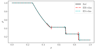
(a) $p=2$, $n_{e}=200$

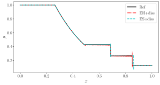
(b) $p=5$, $n_{e}=800$

Figure 1: Density profile for the Sod shock tube problem at $t=0.2$ using the locally conservative hybrid scheme and the nonconservative entropy-split scheme.

Fig. 1 shows that the hybrid scheme captures the correct shock speed while the entropy-split method does not. It is evident from Fig. 1(b) that the entropy-split solution does not converge to the reference solution by refining the mesh or increasing the order of discretization. The numerical solutions oscillate as no limiting or explicit shock capturing methods are employed. Fig. 2(a) shows that both the entropy-split and hybrid schemes conserve entropy for problems with shock waves in the absence of interface dissipation. It can also be concluded from the figure that the amount of dissipation added using the interface dissipation operator, 69, is close to the exact entropy dissipation for this problem. The change in entropy is computed as

$$\Delta s_{t}=\frac{s_{t}-s_{0}}{\absolutevalue{s_{0}}},$$ (102)

where $s_{t}$ and $s_{0}$ are the entropy values at time $t$ and $t=0$ computed as $s=\bm{1}^{T}\mathsf{H}_{g}\bm{s}$. Fig. 2(b) shows that the $\gamma_{n}$ parameter of the RRK method is close to unity for both schemes with or without dissipation.

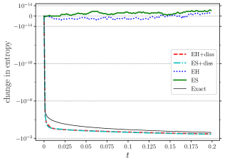
(a) $p=1$, $n_{e}=200$

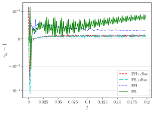
(b) $p=1$, $n_{e}=200$

Figure 2: Change in entropy for the Sod shock tube problem at $t=0.2$ using the hybrid and entropy-split schemes with and without dissipation.

7.2 The Shu-Osher shock tube problem

To further demonstrate that the hybrid scheme captures discontinuities accurately, we solve the Shu-Osher sine wave problem [88], which simulates a normal shock wave propagating into a medium with small sinusoidal density perturbations. The problem is governed by the Euler equations, and the initial conditions are

$$\rho_{L} =3.857143,\quad u_{L} =2.629369,\quad p_{L} =10.33333,\quad \text{if }x \leq-4,$$

$$\rho_{R} =1+0.2\sin(5x),\quad u_{R} =0,\quad p_{R} =1,\quad \text{if }x >-4.$$

The domain is $\Omega=[-5,5]$, the final time is $t_{f}=1.8$, and the CFL value is set to $0.1$. The timestep computation and solution updates are handled in the same manner as for the Sod shock tube problem. For this problem, the Sjögreen-Yee two point flux is applied on all elements between the left and right most shock waves, whose locations are determined from numerical solutions obtained using conservative schemes. At $t=0$, for instance, the conservative scheme is applied on a single or two elements at $x=-4$, while at $t=1.8$ it is applied on elements between $x=-2.8$ and $x=2.5$, covering the region of the domain in which discontinuities are present. The idea is to apply the two-point flux scheme only at critical portions of the domain where discrete conservation is indispensable. Since the exact solution for this problem is not known, we use the $p=3$ Ismail-Roe Hadamard-form discretization with $n_{e}=10000$ to compute the reference solution. A matrix-type dissipation operator of [41] is applied with the IR discretization, while the entropy-split and hybrid schemes use the dissipation operator presented in Section 4.5.

From the density profile depicted in Fig. 3, it is clear that the hybrid scheme captures the small and large shock waves accurately. The entropy-split scheme fails to do so as expected. Increasing the mesh resolution or polynomial degree improves the solution accuracy of the hybrid scheme as illustrated in Fig. 4. Similar to the Sod shock tube problem, the numerical solution is oscillatory as no limiting or shock capturing method is applied.

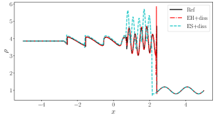
(a) $p=2$, $n_{e}=400$

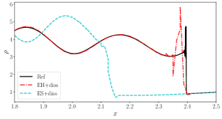
(b) $p=2$, $n_{e}=400$, closeup

Figure 3: Density profile for the Shu-Osher shock tube problem at $t=1.8$ using the locally conservative hybrid scheme and the nonconservative entropy-split scheme.

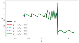
(a) hybrid scheme

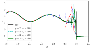
(b) hybrid scheme, closeup

Figure 4: Density profile for the Shu-Osher shock tube problem at $t=1.8$ using the locally conservative hybrid scheme.

7.3 The isentropic vortex problem

The isentropic vortex problem is a smooth problem governed by the Euler equations. Both the 2D and 3D versions of the problem are used to study accuracy, primary conservation, entropy conservation, and efficiency of the proposed scheme. The analytical solution for the 2D case on the domain $\Omega=\left[0,20\right]\times\left[-5,5\right]$ is given as [89, 45],

$$\rho =\left(1-\frac{\alpha^{2}\left(\gamma-1\right)}{16\gamma\pi}\exp\left(2\left(1-r^{2}\right)\right)\right)^{\frac{1}{\gamma-1}}, p =\rho^{\gamma},$$ (103)

$$u =1-\frac{\alpha}{2\pi}\left({\color[rgb]{0,0,0}x_{2}}-y_{c}\right)\exp\left(1-r^{2}\right), v =\frac{\alpha}{2\pi}\left({\color[rgb]{0,0,0}x_{1}}-\left(x_{c}+t\right)\right)\exp\left(1-r^{2}\right),$$

where $r^{2}=\left({\color[rgb]{0,0,0}x_{1}}-x_{c}+t\right)^{2}+\left({\color[rgb]{0,0,0}x_{2}}-y_{c}\right)^{2}$, $\alpha=3$ is the vortex strength, $\left(x_{c},y_{c}\right)=\left(5,0\right)$ is the center of the vortex at $t=0$, and $\gamma=7/5$. The grids are curved using the perturbation [25]

$${\color[rgb]{0,0,0}x_{1}} =\hat{{\color[rgb]{0,0,0}x}}_{1}+\frac{1}{8}\cos\left(\frac{\pi}{20}\left(\hat{x}_{1}-10\right)\right)\cos\left(\frac{3\pi}{10}\hat{{\color[rgb]{0,0,0}x}}_{2}\right), {\color[rgb]{0,0,0}x_{2}} =\hat{{\color[rgb]{0,0,0}x}}_{2}+\frac{1}{8}\sin\left(\frac{\pi}{5}\left({\color[rgb]{0,0,0}x_{1}}-10\right)\right)\cos\left(\frac{\pi}{10}\hat{{\color[rgb]{0,0,0}x}}_{2}\right),$$ (104)

where $(\hat{\cdot})$ denotes the coordinate of a node before perturbation. In 3D, we use the analytical solution [90, 45],

$$\rho =\left(1-\frac{2}{25}\left(\gamma-1\right)\exp\left(1-\left({\color[rgb]{0,0,0}x_{2}}-t\right)^{2}-{\color[rgb]{0,0,0}x}_{1}^{2}\right)\right)^{\frac{1}{\gamma-1}}, e =\frac{\rho^{\gamma}}{\gamma(\gamma-1)}+\frac{\rho}{2}\left({\color[rgb]{0,0,0}V_{1}}^{2}+{\color[rgb]{0,0,0}V_{2}}^{2}+{\color[rgb]{0,0,0}V_{3}}^{2}\right),$$ (105)

$${\color[rgb]{0,0,0}V_{1}} =-\frac{2}{5}\left({\color[rgb]{0,0,0}x_{2}}-t\right)\exp\left(\frac{1}{2}\left[1-\left({\color[rgb]{0,0,0}x_{1}}-t\right)^{2}-{\color[rgb]{0,0,0}x}_{1}^{2}\right]\right), {\color[rgb]{0,0,0}V_{2}} =1+\frac{2}{5}{\color[rgb]{0,0,0}x_{1}}\exp\left(\frac{1}{2}\left[1-\left({\color[rgb]{0,0,0}x_{2}}-t\right)^{2}-{\color[rgb]{0,0,0}x}_{1}^{2}\right]\right), {\color[rgb]{0,0,0}V_{3}} =0.$$

The domain is $\Omega=\left[-10,10\right]^{3}$, and the grids are curved according to the perturbation

$${x}_{i}=\hat{{x}}_{i}+0.05\sin\left(\frac{\pi\hat{{x}}_{i}}{2}\right),\quad\forall i\in\{1,2,3\}.$$ (106)

7.3.1 Accuracy

The high-order accuracy of the entropy-split scheme is validated by running the 2D and 3D isentropic vortex problems on a sequence of curved meshes. In 2D, curved triangular elements are used which are obtained by subdividing rectangular elements into two and applying the perturbation given in 104. Similarly, in 3D, curved tetrahedral elements are obtained by subdividing hexahedral elements into six tetrahedra and applying the perturbation given in 106. We followed the procedure outlined in [45] to compute the $L^{2}$ error, i.e., interpolate the solution from the SBP nodes to a quadrature rule of degree $3p+1$, integrate the square of the solution error, sum the result over all elements, and take the square root of the sum. Given solution errors on two meshes, the convergence rates are computed as $\log(\text{error}_{2}/\text{error}_{1})/\log(h_{2}/h_{1})$, where $h_{i}={(\text{vol.}/n_{e,i})}^{1/d}$ and vol. is either the area or volume of the domain.

The solution convergence results for the 2D problem at $t_{f}=2$ and the 3D case at $t_{f}=1$ are presented in Tables 1 and 2, respectively. CFL values of $0.1$ and $0.25$ are used for the 2D and 3D cases, respectively. For comparison, we have also included the corresponding errors and convergence rates of the Ismail-Roe Hadamard-form discretization. It can be seen from the tables that convergence rates between $p$ and $p+1$ are observed for all cases. In the 2D case, the entropy conservative schemes exhibit an even-odd convergence rate behavior, where the even degree operators converge at rates greater than $p+0.5$ while the odd degree operators converge close to a suboptimal rate of $p$. This behavior has been reported previously, e.g., see [51, 91, 92, 93]. Adding dissipation improves the solution convergence rates for all cases and decreases the solution errors significantly. The solution errors of the entropy-split and Ismail-Roe Hadamard-form schemes are very close, with the latter having slightly lower errors for almost all cases.

Table 1: Grid convergence study for the 2D isentropic vortex problem on curvilinear grids at $t_{f}=2$.

$p$	$n_{e}$	Entropy-split				IR Hadamard-form
		conservative		dissipative		conservative		dissipative
		$L^{2}$ error	rate	$L^{2}$ error	rate	$L^{2}$ error	rate	$L^{2}$ error	rate
$1$	$60^{2}\times 2$	2.7515e-01	–	1.4652e-01	–	2.8223e-01	–	1.5185e-01	–
	$80^{2}\times 2$	2.1770e-01	0.81	8.7858e-02	1.77	2.2491e-01	0.78	9.0908e-02	1.78
	$100^{2}\times 2$	1.7857e-01	0.88	5.8532e-02	1.82	1.8452e-01	0.88	6.0450e-02	1.82
	$120^{2}\times 2$	1.5189e-01	0.88	4.1900e-02	1.83	1.5668e-01	0.89	4.3219e-02	1.84
$2$	$60^{2}\times 2$	1.8342e-02	–	1.0346e-02	–	1.7201e-02	–	1.0074e-02	–
	$80^{2}\times 2$	8.6064e-03	2.63	4.7957e-03	2.67	7.9423e-03	2.68	4.5671e-03	2.74
	$100^{2}\times 2$	4.6965e-03	2.71	2.5913e-03	2.75	4.3051e-03	2.74	2.4300e-03	2.82
	$120^{2}\times 2$	2.8214e-03	2.79	1.5550e-03	2.80	2.5832e-03	2.80	1.4428e-03	2.85
$3$	$60^{2}\times 2$	1.8747e-03	–	8.0180e-04	–	1.9087e-03	–	7.5947e-04	–
	$80^{2}\times 2$	7.3938e-04	3.23	2.8758e-04	3.56	7.6724e-04	3.16	2.7114e-04	3.58
	$100^{2}\times 2$	3.6119e-04	3.21	1.3091e-04	3.52	3.7775e-04	3.17	1.2265e-04	3.55
	$120^{2}\times 2$	1.9582e-04	3.35	6.8669e-05	3.53	2.0658e-04	3.31	6.3942e-05	3.57
$4$	$60^{2}\times 2$	1.6301e-04	–	6.9849e-05	–	1.4134e-04	–	6.7207e-05	–
	$80^{2}\times 2$	4.4338e-05	4.52	1.7623e-05	4.78	3.8150e-05	4.55	1.6995e-05	4.77
	$100^{2}\times 2$	1.6038e-05	4.55	6.0291e-06	4.80	1.3538e-05	4.64	5.8206e-06	4.80
	$120^{2}\times 2$	6.8290e-06	4.68	2.5207e-06	4.78	5.7351e-06	4.71	2.4313e-06	4.78

Table 2: Grid convergence study for the 3D isentropic vortex problem on curvilinear grids at $t_{f}=1$.

$p$	$n_{e}$	Entropy-split				IR Hadamard-form
		conservative		dissipative		conservative		dissipative
		$L^{2}$ error	rate	$L^{2}$ error	rate	$L^{2}$ error	rate	$L^{2}$ error	rate
$1$	$15^{3}\times 6$	1.1982e+00	–	1.2204e+00	–	1.2120e+00	–	1.2298e+00	–
	$20^{3}\times 6$	7.5842e-01	1.58	7.4754e-01	1.70	7.5699e-01	1.63	7.4465e-01	1.74
	$25^{3}\times 6$	5.2297e-01	1.66	4.9881e-01	1.81	5.2184e-01	1.66	4.9923e-01	1.79
	$30^{3}\times 6$	3.7637e-01	1.80	3.5070e-01	1.93	3.7653e-01	1.79	3.5056e-01,	1.93
$2$	$15^{3}\times 6$	3.7061e-01	–	3.3001e-01	–	3.6917e-01	–	3.2805e-01	–
	$20^{3}\times 6$	1.7847e-01	2.54	1.5410e-01	2.64	1.7721e-01	2.55	1.5354e-01	2.63
	$25^{3}\times 6$	9.4926e-02	2.82	8.1664e-02	2.84	9.3071e-02	2.88	8.0866e-02	2.87
	$30^{3}\times 6$	5.9186e-02	2.59	4.9042e-02	2.79	5.7696e-02	2.62	4.8443e-02	2.81
$3$	$15^{3}\times 6$	1.2425e-01	–	9.5332e-02	–	1.1558e-01	–	9.3329e-02	–
	$20^{3}\times 6$	4.6054e-02	3.45	3.7759e-02	3.21	4.4596e-02	3.31	3.6779e-02	3.23
	$25^{3}\times 6$	2.2157e-02	3.27	1.6972e-02	3.58	2.1349e-02	3.30	1.6885e-02	3.48
	$30^{3}\times 6$	1.1566e-02	3.56	8.5225e-03	3.77	1.0965e-02	3.65	8.3907e-03	3.83
$4$	$15^{3}\times 6$	3.8613e-02	–	2.7985e-02	–	3.5419e-02	–	2.7259e-02	–
	$20^{3}\times 6$	1.2417e-02	3.94	8.4335e-03	4.16	1.1120e-02	4.02	7.9801e-03	4.27
	$25^{3}\times 6$	4.7588e-03	4.29	2.9824e-03	4.65	4.1733e-03	4.39	2.7874e-03	4.71
	$30^{3}\times 6$	2.0922e-03	4.50	1.2713e-03	4.67	1.8952e-03	4.32	1.2137e-03	4.56

7.3.2 Primary conservation

We investigate the convergence of the primary conservation error with mesh refinement for the entropy-split scheme, where the conservation error is computed as

$$\text{error}=\frac{\absolutevalue{\left[\sum_{\Omega_{k}\in\mathcal{T}_{h}}\overline{\mathsf{I}}^{T}\overline{\mathsf{H}}_{k}\bm{u}_{k}\right]_{t=t_{f}}-\left[\sum_{\Omega_{k}\in\mathcal{T}_{h}}\overline{\mathsf{I}}^{T}\overline{\mathsf{H}}_{k}\bm{u}_{k}\right]_{t=0}}}{\absolutevalue{\left[\sum_{\Omega_{k}\in\mathcal{T}_{h}}\overline{\mathsf{I}}^{T}\overline{\mathsf{H}}_{k}\bm{u}_{k}\right]_{t=0}}}.$$

The entropy-split scheme is not conservative, but the conservation errors in mass, momentum, and energy decrease quickly with mesh refinement for smooth solutions. The convergence of mass and energy conservation errors for the 2D and 3D entropy-split discretizations of the isentropic vortex problems is reported in Table 3. We observe superconvergence rates close to or greater than $2p$ for both quantities in almost all cases, which is in accordance with Remark 4. This is an encouraging property of the entropy-split scheme as it allows the loss of conservation to be mitigated with modest mesh refinement compared to what would have been needed if the convergence rate was limited to $p+1$. Although not reported, we have observed similar superconvergence behavior for the conservation of momentum in each direction.

Table 3: Mass and energy conservation grid convergence study for the isentropic vortex problems.

$p$	2D ES scheme					3D ES scheme
	$n_{e}$	mass		energy		$n_{e}$	mass		energy
		error	rate	error	rate		error	rate	error	rate
$1$	$60^{2}\times 2$	6.0705e-06	–	1.1264e-05	–	$15^{3}\times 6$	3.8546e-06	–	8.3150e-06	–
	$80^{2}\times 2$	1.7304e-06	4.36	1.5949e-06	6.80	$20^{3}\times 6$	1.5919e-06	3.07	3.0643e-06	3.47
	$100^{2}\times 2$	2.7436e-07	8.25	1.3462e-06	0.76	$25^{3}\times 6$	1.0567e-06	1.84	2.0954e-06	1.70
	$120^{2}\times 2$	1.6641e-07	2.74	1.9304e-06	$-1.98^{\dagger}$	$30^{3}\times 6$	7.1835e-07	2.12	1.3534e-06	2.40
$2$	$60^{2}\times 2$	1.3948e-07	–	3.1346e-07	–	$15^{3}\times 6$	1.1523e-06	–	2.1950e-06	–
	$80^{2}\times 2$	2.9296e-08	5.42	7.2323e-08	5.10	$20^{3}\times 6$	4.8005e-07	3.04	9.1724e-07	3.03
	$100^{2}\times 2$	9.1568e-09	5.21	2.4679e-08	4.82	$25^{3}\times 6$	2.0123e-07	3.90	3.8547e-07	3.89
	$120^{2}\times 2$	3.4885e-09	5.29	1.0153e-08	4.87	$30^{3}\times 6$	8.7548e-08	4.56	1.6570e-07	4.63
$3$	$60^{2}\times 2$	2.8481e-09	–	6.0358e-09	–	$15^{3}\times 6$	2.9194e-07	–	4.8042e-07	–
	$80^{2}\times 2$	4.9214e-10	6.10	1.0529e-09	6.07	$20^{3}\times 6$	6.4213e-08	5.26	4.8042e-07	4.93
	$100^{2}\times 2$	1.3194e-10	5.90	2.8771e-10	5.81	$25^{3}\times 6$	1.5399e-08	6.40	4.8042e-07	6.76
	$120^{2}\times 2$	4.1898e-11	6.29	9.3279e-11	6.18	$30^{3}\times 6$	5.1313e-09	6.03	4.8042e-07	5.96
$4$	$60^{2}\times 2$	3.3298e-11	–	6.9952e-11	–	$15^{3}\times 6$	5.8265e-08	–	4.8042e-07	–
	$80^{2}\times 2$	2.6775e-12	8.76	5.5775e-12	8.79	$20^{3}\times 6$	6.9086e-09	7.41	4.8042e-07	7.49
	$100^{2}\times 2$	3.8784e-13	8.66	7.9809e-13	8.71	$25^{3}\times 6$	1.2298e-09	7.73	2.0520e-09	7.81
	$120^{2}\times 2$	8.4176e-14	8.38	1.5320e-13	9.05	$30^{3}\times 6$	2.4543e-10	8.84	4.0164e-10	8.95

• ^†Upon further mesh refinement, the convergence rate of the error in energy conservation is found to be approximately $2$.

7.3.3 Long-time entropy conservation and error behavior

To study the long-time entropy conservation and error behavior of the entropy-split discretization, we run the 2D isentropic vortex problem until $t_{f}=1000$, which corresponds to $50$ revolutions of the vortex. For this case, the CFL is set to $0.5$ and a coarse mesh with a total of $n_{e}=800$ curved elements is used. The results are shown in Fig. 5. The entropy is conserved for all cases until the end of the simulation or termination due to instabilities. For $\beta=2.5$, the odd degree cases run until the final time, while the even degree cases crash before the end of the simulation. Reducing the CFL value by an order of magnitude did not resolve the issue. The cause of instability is not clear, but it seems to be associated with the value of $\beta$. Figs. 5(c) and 5(d) show that for $\beta=2$, all cases run until the end of the simulation except for the $p=1$ case, which suggests that further research is required to choose the values of $\beta$ systematically. When interface dissipation is added, all cases run until the end of the simulation for both $\beta=2.5$ and $\beta=2$ cases. We have also tested the long-time entropy conservation and error behavior of the Ismail-Roe Hadamard-form discretization. We found that the scheme conserves entropy until the final time, and no instability is encountered for all cases. Furthermore, we note that the error values are comparable to those obtained with the entropy-split scheme.

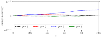
(a) $\beta=2.5$

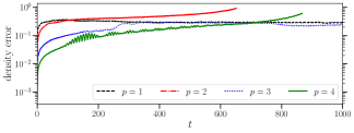
(b) $\beta=2.5$

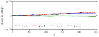
(c) $\beta=2$

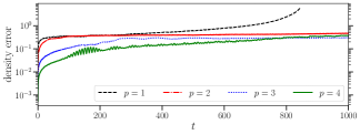
(d) $\beta=2$

Figure 5: Long time entropy conservation and error behavior of the entropy-split method applied for the two dimensional isentropic vortex problem using $n_{e}=800$ curved elements and $\text{CFL}=0.5$.

7.3.4 Efficiency

One of the appealing aspects of the entropy-split scheme is its efficiency. As described in Section 6.3, for implementations with multidimensional SBP operators, the cost of computing the entropy-split discretization of the inviscid flux derivatives is lower than the corresponding cost of the Hadamard-form scheme. The efficiency depends on factors such as the type of operators used, the use of tensor-product structure, the SATs, code optimization, and many other implementation details. We have attempted to make fair comparisons between the methods by running both the entropy-split and Hadamard form implementations within a single code base; only the computation of the inviscid flux derivatives is handled with different subroutines. A number of optimization techniques recommended in [24] for the Hadamard-form scheme are applied (see, Section 6.3), and similar level of optimization is applied for the entropy-split scheme.

The 3D isentropic vortex problem discretized with multidimensional diagonal-$\mathsf{E}$ operators is used for the efficiency comparison. Only the costs of computing the spatial residuals are compared, and other implementation specific computational costs such as operator construction and time marching are not included. Furthermore, only serial performance is reported. The problem is run for $50$ timesteps with $n_{e}=750$, and the average performance of each scheme over five runs normalized by the average runtime of the Ismail-Roe Hadamard-form scheme is illustrated in Fig. 6. It can be seen from the figure that as the degree of operators increases the computational cost of the Hadamard-form implementation increases quickly, while the entropy-split scheme scales well for implementations with high-order operators. For the degree three and four cases, the computational cost of the spatial residual terms with the entropy-split scheme is about $2$ and $3$ times less expensive, respectively, compared to the Ismail-Roe Hadamard-form implementation.

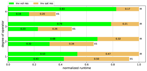
Figure 6: Efficiency comparisons of the entropy-split scheme and the Ismail-Roe Hadamard-form discretization of the 3D isentropic vortex problem.

7.4 Manufactured solution for the compressible Navier-Stokes equations

The method of manufactured solutions is used to test the accuracy of the entropy-split discretization of the compressible Navier-Stokes equations. To this end, we use the manufactured solution [94]

$$\rho =2.0+0.1\sin(\pi\left(\Sigma_{i=1}^{d}\bm{x}_{i}-0.6t\right)), \quad V_{i} =1, \quad p =(\gamma-1)(\rho^{2}-0.5\rho\bm{V}^{T}\bm{V}),\quad i=\{1,\dots,d\},$$

defined on the periodic domain $\Omega=[-1,1]^{d}$. The domain is discretized with SBP diagonal-$\mathsf{E}$ elements which are curved according to the mapping [95]

$$\bm{x}_{i} =\hat{\bm{x}}_{i}+\frac{1}{8}\cos\left(\frac{\pi}{2}\hat{\bm{x}}_{i}\right)\prod_{j=1,j\neq i}^{d}\sin\left(\pi\hat{\bm{x}}_{j}\right),\quad i=\{1,\dots,d\}.$$ (107)

The source terms are obtained by substituting the manufactured solution into the compressible Navier-Stokes equations, 4, and solving for the difference of the left and right hand sides. A constant viscosity, $\mu=0.01$, is used, the gas constant and Prandtl number are set to $R=1$ and $Pr=0.71$, respectively. The BO SAT coefficients given in 96 are used to couple the viscous terms at element interfaces. No interface dissipation is added with either the inviscid or viscous SATs.

Both the 2D and 3D cases are run for $1000$ timesteps until the final time, $t_{f}=0.001$. Table 4 shows the $L^{2}$ solution error and convergence rates obtained with the entropy-split and Ismail-Roe Hadamard-form discretizations. We observe convergence rates of approximately $p+1$ for all cases. Furthermore, the error values obtained with the two schemes are comparable.

Table 4: Grid convergence study for the manufactured solution of the compressible Navier-Stokes equations at $t_{f}=0.001$.

$p$	2D					3D
	$n_{e}$	ES scheme		IR scheme		$n_{e}$	ES scheme		IR scheme
		$L^{2}$ error	rate	$L^{2}$ error	rate		$L^{2}$ error	rate	$L^{2}$ error	rate
$1$	$20^{2}\times 2$	2.8996e-03	–	2.8992e-03	–	$6^{3}\times 6$	1.5492e-01	–	1.5492e-01	–
	$30^{2}\times 2$	1.2991e-03	1.98	1.2988e-03	1.98	$9^{3}\times 6$	7.2321e-02	1.87	7.2323e-02	1.87
	$40^{2}\times 2$	7.3772e-04	1.96	7.3744e-04	1.96	$12^{3}\times 6$	4.1432e-02	1.93	4.1434e-02	1.93
	$50^{2}\times 2$	4.7759e-04	1.94	4.7732e-04	1.94	$15^{3}\times 6$	2.6749e-02	1.96	2.6751e-02	1.96
$2$	$20^{2}\times 2$	9.7812e-05	–	9.7827e-05	–	$6^{3}\times 6$	3.4847e-02	–	3.4845e-02	–
	$30^{2}\times 2$	2.8970e-05	3.00	2.8966e-05	3.00	$9^{3}\times 6$	1.1110e-02	2.81	1.1110e-02	2.81
	$40^{2}\times 2$	1.2199e-05	3.00	1.2192e-05	3.00	$12^{3}\times 6$	4.8167e-03	2.90	4.8179e-03	2.90
	$50^{2}\times 2$	6.2329e-06	3.00	6.2266e-06	3.00	$15^{3}\times 6$	2.4989e-03	2.94	2.5002e-03	2.93
$3$	$20^{2}\times 2$	2.4811e-06	–	2.4811e-06	–	$6^{3}\times 6$	7.0398e-03	–	7.0223e-03	–
	$30^{2}\times 2$	4.9958e-07	3.95	4.9848e-07	3.96	$9^{3}\times 6$	1.5260e-03	3.77	1.5209e-03	3.77
	$40^{2}\times 2$	1.6181e-07	3.91	1.6099e-07	3.92	$12^{3}\times 6$	5.0177e-04	3.86	4.9936e-04	3.87
	$50^{2}\times 2$	6.8144e-08	3.87	6.7564e-08	3.89	$15^{3}\times 6$	2.0991e-04	3.90	2.0852e-04	3.91
$4$	$20^{2}\times 2$	5.8660e-08	–	5.7522e-08	–	$6^{3}\times 6$	1.3981e-03	–	1.3417e-03	–
	$30^{2}\times 2$	8.0093e-09	4.91	7.6089e-09	4.98	$9^{3}\times 6$	2.1934e-04	4.56	2.0216e-04	4.66
	$40^{2}\times 2$	1.9966e-09	4.82	1.8194e-09	4.97	$12^{3}\times 6$	5.6838e-05	4.69	5.0252e-05	4.83
	$50^{2}\times 2$	6.9568e-10	4.72	6.0473e-10	4.93	$15^{3}\times 6$	1.9956e-05	4.69	1.6842e-05	4.89

7.5 Viscous Taylor-Green vortex

The Taylor-Green vortex problem is a challenging test case frequently used to study the accuracy and robustness of high-order numerical methods. For many schemes, the simulation of stretching large scale eddies breaking down into smaller eddies which are eventually dissipated due to viscosity requires a careful application of artificial dissipation or other ad-hoc stabilization techniques. Maintaining a balance between the amount of dissipation required for stability and the amount that can be added without compromising accuracy is challenging. Entropy stable high-order methods offer enhanced stability properties that eliminate the need to use ad-hoc stabilization methods. Our goal is to investigate whether the entropy-split scheme, despite not being provably entropy stable for the compressible Navier-Stokes equations, remains practically stable for the under-resolved Taylor-Green vortex problem, and whether it provides an accurate solution for a well-resolved case. We also present how the efficiency of the entropy-split scheme for viscous flows compares with that of the Hadamard-form discretization.

The viscous Taylor-Green vortex problem is defined on the domain $\Omega=\left[-\pi,\pi\right]^{3}$ with the initial conditions [96]

$${\color[rgb]{0,0,0}V_{1}} =u_{0}\sin\left(\frac{{\color[rgb]{0,0,0}x_{1}}}{L}\right)\cos\left(\frac{{\color[rgb]{0,0,0}x_{2}}}{L}\right)\cos\left(\frac{{\color[rgb]{0,0,0}x_{3}}}{L}\right), \quad p =p_{0}+\frac{\rho_{0}u_{0}^{2}}{16}\left[\cos\left(\frac{2{\color[rgb]{0,0,0}x_{1}}}{L}\right)+\cos\left(\frac{2{\color[rgb]{0,0,0}x_{2}}}{L}\right)\right]\left[\cos\left(\frac{2{\color[rgb]{0,0,0}x_{3}}}{L}\right)+2\right], \quad\rho =\frac{p}{RT_{0}},$$

$${\color[rgb]{0,0,0}V_{2}} =-u_{0}\cos\left(\frac{{\color[rgb]{0,0,0}x_{1}}}{L}\right)\sin\left(\frac{{\color[rgb]{0,0,0}x_{2}}}{L}\right)\cos\left(\frac{{\color[rgb]{0,0,0}x_{3}}}{L}\right), \quad{\color[rgb]{0,0,0}V_{3}} =0,$$

where $u_{0}=\rho_{0}=R=L=1$, $T_{0}=p_{0}/(R\rho_{0})$, $M=u_{0}/\sqrt{\gamma RT_{0}}=0.1$ is the Mach number, and $p_{0}=\rho_{0}u_{0}^{2}/(\gamma M^{2})$. The Reynolds number is $Re=\rho_{0}u_{0}L/\mu_{0}=\{100,200\}$, where $\mu_{0}$ is a constant viscosity, and the Prandtl number is set to $Pr=0.71$. The scaled kinetic energy is computed as

$$E_{k}=\frac{1}{\rho_{0}\left|\Omega\right|}\int_{\Omega}\rho\frac{\bm{V}\cdot\bm{V}}{2}\differential{\Omega},$$ (108)

where $\left|\Omega\right|=8\pi^{3}$, and the kinetic energy dissipation rate is given by

$$\varepsilon=-\dfrac{{\rm d}E_{k}}{{\rm d}t},$$ (109)

which is computed using the fifth-order classical SBP derivative operator.

The problem is solved on tetrahedral meshes with approximately $64^{3}$ and $128^{3}$ degrees of freedom (DOF) for $Re=100$ and $Re=200$ cases, respectively. The standard RK4 method is used for time marching. Despite not being provably entropy stable for the compressible Navier-Stokes equations, the entropy-split scheme remains stable when applied to this challenging test case, including at larger Reynolds numbers, e.g., $Re=1600$. Fig. 7 shows that the kinetic energy dissipation rates obtained using the entropy-split scheme match the DNS results of Brachet et al. [97] reasonably well. For larger values of Reynolds number, the DOFs required to resolve the flow accurately using the SBP diagonal-$\mathsf{E}$ tetrahedral elements increases quickly. A further investigation on the accuracy of the operators is left for future research.

An efficiency comparison of the entropy-split and Ismail-Roe Hadamard-form discretizations for the viscous Taylor-Green vortex is depicted in Fig. 8. Again, the normalized average serial performance over five runs, each consisting of 20 timesteps with $n_{e}=750$ elements, is reported. While the entropy-split scheme is more efficient than the Ismail-Roe Hadamard-form scheme, the efficiency benefit is not as significant as it is for the Euler equations due to the dominant cost of the viscous terms. However, it is evident from the figure that the proportional cost of the viscous terms is decreasing with increasing operator degree. Hence, for very high degree operators, the efficiency benefit of the entropy-split scheme can be substantial for the compressible Navier-Stokes equations.

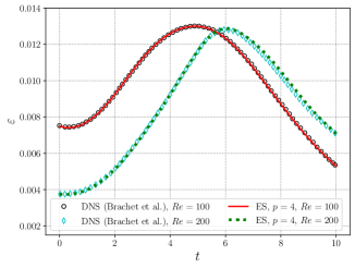
Figure 7: Kinetic energy dissipation rate of the viscous Taylor-Green vortex problem solved with the entropy-split scheme using approximately $64^{3}$ and $128^{3}$ DOFs for the $Re=100$ and $Re=200$ cases, respectively.

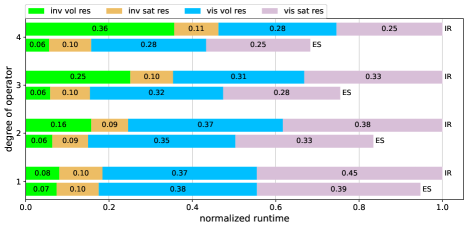
Figure 8: Efficiency comparisons of the entropy-split and Ismail-Roe Hadamard-form discretizations of the viscous Taylor-Green vortex problem.

8 Conclusions

The entropy-split scheme is extended to element-type implementations using diagonal-norm diagonal-$\mathsf{E}$ multidimensional SBP operators and entropy conservative SATs. We show that the scheme is high order accurate and entropy conservative on periodic curvilinear grids for the Euler equations. Its entropy stability does not extend to the compressible Navier-Stokes equations unless heat fluxes are neglected. Neglecting heat fluxes and applying appropriate viscous SATs, however, we show that the entropy-split scheme is entropy stable for the compressible Navier-Stokes equations. The viscous SATs are also applicable to existing Hadamard-form discretizations, and they are extensions of the SATs presented in [35, 36] to systems of equations with a symmetric positive semidefinite diffusivity tensor.

The entropy-split scheme is inherently not conservative in the sense of Lax-Wendroff. To mitigate the effects of this loss of conservation, an entropy stable hybrid scheme consisting of the entropy-split and Sjögreen-Yee Hadamard-form discretizations is proposed. The hybrid scheme is locally conservative, and numerical results show that it converges to the correct weak solution. A matrix-form interface dissipation operator is designed to provide entropy dissipation for the hybrid, entropy-split, and Sjögreen-Yee Hadamard-form schemes.

The high-order accuracy of the entropy-split scheme is verified using problems governed by the Euler and Navier-Stokes equations. We found that the solutions to the problems considered converge at rates between $p$ and $p+1$ under mesh refinement. Furthermore, for the entropy-split scheme, the primary conservation errors superconverge at rates close to $2p$. For long time simulations of the isentropic vortex problem, we observed that the stability of the entropy-split scheme depends on the value of the arbitrary splitting parameter $\beta$. However, the stability issues disappear if interface matrix-dissipation is applied. Despite not being entropy stable for the Navier-Stokes equations, no practical instability is observed with the entropy-split scheme when applied to the challenging viscous Taylor-Green vortex problem. In practice, the entropy-split scheme is applied with the heat fluxes included, and despite not being provably entropy stable in this case, the method is likely to be more robust than the standard divergence form discretization for many problems, as the heat fluxes are rarely the source of difficulties in numerical simulations. In general, however, it can be concluded that the entropy-split scheme is less robust than the Ismail-Roe Hadamard-form scheme due to the problem dependent $\beta$ parameter, and further research is required to mitigate this robustness issue.

Finally, efficiency comparison tests show that the computational costs of the spatial residual terms of the Euler equations with the entropy-split scheme using the degree three and four SBP diagonal-$\mathsf{E}$ tetrahedral elements are, respectively, about two and three times smaller than the corresponding costs with the Ismail-Roe Hadamard form scheme. The efficiency benefit for the Navier-Stokes equations is not as large due to the dominant cost of the viscous terms. However, based on the observation that the proportional cost of the viscous terms is decreasing for increasing operator degree, the efficiency benefit of the entropy-split method for the Navier-Stokes equations compared to the Hadamard-form scheme can be substantial for very high order discretizations.

Declaration of competing interest

The authors declare that they have no known competing financial interests or personal relationships that could have appeared to influence the work reported in this paper.

References

- Sjögreen and Yee [2019] B. Sjögreen, H. Yee, Entropy stable method for the Euler equations revisited: central differencing via entropy splitting and SBP, Journal of Scientific Computing 81 (2019) 1359–1385.
- Yee and Sjögreen [2023] H. Yee, B. Sjögreen, Recent advancement of entropy split methods for compressible gas dynamics and MHD, Applied Mathematics and Computation 439 (2023) 127545.
- Sjögreen and Yee [2021] B. Sjögreen, H. Yee, Construction of conservative numerical fluxes for the entropy split method, Communications on Applied Mathematics and Computation (2021) 1–26.
- Nordström [2022a] J. Nordström, Nonlinear and linearised primal and dual initial boundary value problems: When are they bounded? How are they connected?, Journal of Computational Physics 455 (2022a) 111001.
- Nordström [2022b] J. Nordström, A skew-symmetric energy and entropy stable formulation of the compressible Euler equations, Journal of Computational Physics 470 (2022b) 111573.
- Fisher and Carpenter [2013] T. C. Fisher, M. H. Carpenter, High-order entropy stable finite difference schemes for nonlinear conservation laws: Finite domains, Journal of Computational Physics 252 (2013) 518–557.
- Fisher et al. [2013] T. C. Fisher, M. H. Carpenter, J. Nordström, N. K. Yamaleev, C. Swanson, Discretely conservative finite-difference formulations for nonlinear conservation laws in split form: Theory and boundary conditions, Journal of Computational Physics 234 (2013) 353–375.
- Carpenter et al. [2014] M. H. Carpenter, T. C. Fisher, E. J. Nielsen, S. H. Frankel, Entropy stable spectral collocation schemes for the Navier–Stokes equations: Discontinuous interfaces, SIAM Journal on Scientific Computing 36 (2014) B835–B867.
- Chen and Shu [2017] T. Chen, C.-W. Shu, Entropy stable high order discontinuous Galerkin methods with suitable quadrature rules for hyperbolic conservation laws, Journal of Computational Physics 345 (2017) 427–461.
- Crean et al. [2018] J. Crean, J. E. Hicken, D. C. Del Rey Fernández, D. W. Zingg, M. H. Carpenter, Entropy-stable summation-by-parts discretization of the Euler equations on general curved elements, Journal of Computational Physics 356 (2018) 410–438.
- Parsani et al. [2015] M. Parsani, M. H. Carpenter, E. J. Nielsen, Entropy stable discontinuous interfaces coupling for the three-dimensional compressible Navier-Stokes equations., J. Comput. Physics 290 (2015) 132–138.
- Rojas et al. [2021] D. Rojas, R. Boukharfane, L. Dalcin, D. C. Del Rey Fernández, H. Ranocha, D. E. Keyes, M. Parsani, On the robustness and performance of entropy stable collocated discontinuous Galerkin methods, Journal of Computational Physics 426 (2021) 109891.
- Parsani et al. [2021] M. Parsani, R. Boukharfane, I. R. Nolasco, D. C. Del Rey Fernández, S. Zampini, B. Hadri, L. Dalcin, High-order accurate entropy-stable discontinuous collocated Galerkin methods with the summation-by-parts property for compressible CFD frameworks: Scalable SSDC algorithms and flow solver, Journal of Computational Physics 424 (2021) 109844.
- Chan et al. [2022a] J. Chan, H. Ranocha, A. M. Rueda-Ramírez, G. Gassner, T. Warburton, On the entropy projection and the robustness of high order entropy stable discontinuous Galerkin schemes for under-resolved flows, Frontiers in Physics (2022a) 356.
- Chan et al. [2022b] J. Chan, Y. Lin, T. Warburton, Entropy stable modal discontinuous Galerkin schemes and wall boundary conditions for the compressible Navier-Stokes equations, Journal of Computational Physics 448 (2022b) 110723.
- Parsani et al. [2021] M. Parsani, R. Boukharfane, I. E. Reyna Nolasco, L. Dalcin, D. E. Keyes, Simulation of turbulent flows using a fully discrete explicit hp-nonconforming entropy stable solver of any order on unstructured grids, in: AIAA Scitech 2021 Forum, AIAA 2021-0495, 2021.
- Bergmann et al. [2020] M. Bergmann, C. Morsbach, G. Ashcroft, Assessment of split form nodal discontinuous Galerkin schemes for the les of a low pressure turbine profile, in: ERCOFTAC Workshop Direct and Large Eddy Simulation, Springer, 2020, pp. 365–371.
- Yamaleev and Upperman [2022] N. K. Yamaleev, J. Upperman, Positivity-preserving entropy stable schemes for the 1-d compressible Navier-Stokes equations: High-order flux limiting, Journal of Computational Physics 466 (2022) 111354.
- Lin et al. [2023] Y. Lin, J. Chan, I. Tomas, A positivity preserving strategy for entropy stable discontinuous Galerkin discretizations of the compressible Euler and Navier-Stokes equations, Journal of Computational Physics 475 (2023) 111850.
- Parsani et al. [2015] M. Parsani, M. H. Carpenter, E. J. Nielsen, Entropy stable wall boundary conditions for the three-dimensional compressible Navier–Stokes equations, Journal of Computational Physics 292 (2015) 88–113.
- Svard et al. [2018] M. Svard, M. H. Carpenter, M. Parsani, Entropy stability and the no-slip wall boundary condition, SIAM Journal on Numerical Analysis 56 (2018) 256–273.
- Dalcin et al. [2019] L. Dalcin, D. Rojas, S. Zampini, D. C. Del Rey Fernández, M. H. Carpenter, M. Parsani, Conservative and entropy stable solid wall boundary conditions for the compressible Navier–Stokes equations: Adiabatic wall and heat entropy transfer, Journal of Computational Physics 397 (2019) 108775.
- Svärd [2021] M. Svärd, Entropy stable boundary conditions for the Euler equations, Journal of Computational Physics 426 (2021) 109947.
- Ranocha et al. [2023] H. Ranocha, M. Schlottke-Lakemper, J. Chan, A. M. Rueda-Ramírez, A. R. Winters, F. Hindenlang, G. J. Gassner, Efficient implementation of modern entropy stable and kinetic energy preserving discontinuous Galerkin methods for conservation laws, ACM Trans. Math. Softw. (2023). Just Accepted.
- Chan et al. [2019] J. Chan, D. C. Del Rey Fernández, M. H. Carpenter, Efficient entropy stable Gauss collocation methods, SIAM Journal on Scientific Computing 41 (2019) A2938–A2966.
- Gerritsen and Olsson [1996] M. Gerritsen, P. Olsson, Designing an efficient solution strategy for fluid flows: 1. A stable high order finite difference scheme and sharp shock resolution for the Euler equations, Journal of Computational Physics 129 (1996) 245–262.
- Yee et al. [2000] H. C. Yee, M. Vinokur, M. J. Djomehri, Entropy splitting and numerical dissipation, Journal of Computational Physics 162 (2000) 33–81.
- Harten [1983] A. Harten, On the symmetric form of systems of conservation laws with entropy, Journal of computational physics 49 (1983).
- Olsson and Oliger [1994] P. Olsson, J. Oliger, Energy and maximum norm estimates for nonlinear conservation laws, Technical Report, 1994.
- Strand [1994] B. Strand, Summation by parts for finite difference approximations for d/dx, Journal of Computational Physics 110 (1994) 47–67.
- Svärd and Mishra [2012] M. Svärd, S. Mishra, Entropy stable schemes for initial-boundary-value conservation laws, Zeitschrift für angewandte Mathematik und Physik 63 (2012) 985–1003.
- Sjögreen and Yee [2018] B. Sjögreen, H. Yee, High order entropy conservative central schemes for wide ranges of compressible gas dynamics and MHD flows, Journal of Computational Physics 364 (2018) 153–185.
- Hicken et al. [2016] J. E. Hicken, D. C. Del Rey Fernández, D. W. Zingg, Multidimensional summation-by-parts operators: General theory and application to simplex elements, SIAM Journal on Scientific Computing 38 (2016) A1935–A1958.
- Carpenter et al. [1994] M. H. Carpenter, D. Gottlieb, S. Abarbanel, Time-stable boundary conditions for finite-difference schemes solving hyperbolic systems: methodology and application to high-order compact schemes, Journal of Computational Physics 111 (1994) 220–236.
- Yan et al. [2018] J. Yan, J. Crean, J. E. Hicken, Interior penalties for summation-by-parts discretizations of linear second-order differential equations, Journal of Scientific Computing 75 (2018) 1385–1414.
- Worku and Zingg [2021] Z. A. Worku, D. W. Zingg, Simultaneous approximation terms and functional accuracy for diffusion problems discretized with multidimensional summation-by-parts operators, Journal of Computational Physics 445 (2021) 110634.
- Gassner et al. [2018] G. J. Gassner, A. R. Winters, F. J. Hindenlang, D. A. Kopriva, The BR1 scheme is stable for the compressible Navier–Stokes equations, Journal of Scientific Computing 77 (2018) 154–200.
- Chen and Shu [2020] T. Chen, C.-W. Shu, Review of entropy stable discontinuous Galerkin methods for systems of conservation laws on unstructured simplex meshes, CSIAM Transactions on Applied Mathematics 1 (2020) 1–52.
- Lax and Wendroff [1960] P. Lax, B. Wendroff, Systems of conservation laws, Communications on Pure and Applied Mathematics 13 (1960) 217–237.
- Hou and LeFloch [1994] T. Y. Hou, P. G. LeFloch, Why nonconservative schemes converge to wrong solutions: error analysis, Mathematics of computation 62 (1994) 497–530.
- Ismail and Roe [2009] F. Ismail, P. L. Roe, Affordable, entropy-consistent Euler flux functions II: Entropy production at shocks, Journal of Computational Physics 228 (2009) 5410–5436.
- Derigs et al. [2017] D. Derigs, A. R. Winters, G. J. Gassner, S. Walch, A novel averaging technique for discrete entropy-stable dissipation operators for ideal MHD, Journal of Computational Physics 330 (2017) 624–632.
- Winters et al. [2017] A. R. Winters, D. Derigs, G. J. Gassner, S. Walch, A uniquely defined entropy stable matrix dissipation operator for high Mach number ideal MHD and compressible Euler simulations, Journal of Computational Physics 332 (2017) 274–289.
- Ranocha et al. [2020] H. Ranocha, M. Sayyari, L. Dalcin, M. Parsani, D. I. Ketcheson, Relaxation Runge–Kutta methods: Fully discrete explicit entropy-stable schemes for the compressible Euler and Navier–Stokes equations, SIAM Journal on Scientific Computing 42 (2020) A612–A638.
- Shadpey and Zingg [2020] S. Shadpey, D. W. Zingg, Entropy-stable multidimensional summation-by-parts discretizations on hp-adaptive curvilinear grids for hyperbolic conservation laws, Journal of Scientific Computing 82 (2020) 70.
- Del Rey Fernández et al. [2018] D. C. Del Rey Fernández, J. E. Hicken, D. W. Zingg, Simultaneous approximation terms for multi-dimensional summation-by-parts operators, Journal of Scientific Computing 75 (2018) 83–110.
- Del Rey Fernández et al. [2014] D. C. Del Rey Fernández, J. E. Hicken, D. W. Zingg, Review of summation-by-parts operators with simultaneous approximation terms for the numerical solution of partial differential equations, Computers & Fluids 95 (2014) 171–196.
- Svärd and Nordström [2014] M. Svärd, J. Nordström, Review of summation-by-parts schemes for initial–boundary-value problems, Journal of Computational Physics 268 (2014) 17–38.
- Gassner [2013] G. J. Gassner, A skew-symmetric discontinuous Galerkin spectral element discretization and its relation to SBP-SAT finite difference methods, SIAM Journal on Scientific Computing 35 (2013) A1233–A1253.
- Del Rey Fernández et al. [2014] D. C. Del Rey Fernández, P. D. Boom, D. W. Zingg, A generalized framework for nodal first derivative summation-by-parts operators, Journal of Computational Physics 266 (2014) 214–239.
- Carpenter et al. [2015] M. H. Carpenter, M. Parsani, T. C. Fisher, E. J. Nielsen, Entropy stable staggered grid spectral collocation for the Burgers’ and compressible Navier-Stokes equations, NASA TM-2015-218990 (2015).
- Gokcen and Reddy [1996] N. A. Gokcen, R. G. Reddy, Thermodynamics, Springer Science & Business Media, 1996.
- Lomax et al. [2013] H. Lomax, T. H. Pulliam, D. W. Zingg, Fundamentals of computational fluid dynamics, Springer Science & Business Media, 2013.
- Hughes et al. [1986] T. J. Hughes, L. P. Franca, M. Mallet, A new finite element formulation for computational fluid dynamics: I. Symmetric forms of the compressible Euler and Navier-Stokes equations and the second law of thermodynamics, Computer methods in applied mechanics and engineering 54 (1986) 223–234.
- Hauke et al. [2006] G. Hauke, A. Landaberea, I. Garmendia, J. Canales, On the thermodynamics, stability and hierarchy of entropy functions in fluid flow, Computer Methods in Applied Mechanics and Engineering 195 (2006) 4473–4489.
- Godunov [1961] S. K. Godunov, An interesting class of quasilinear systems, in: Dokl. Acad. Nauk SSSR, volume 139, 1961, pp. 521–523.
- Mock [1980] M. S. Mock, Systems of conservation laws of mixed type, Journal of Differential equations 37 (1980) 70–88.
- Tadmor [1987] E. Tadmor, The numerical viscosity of entropy stable schemes for systems of conservation laws. I, Mathematics of Computation 49 (1987) 91–103.
- Ranocha [2018] H. Ranocha, Comparison of some entropy conservative numerical fluxes for the Euler equations, Journal of Scientific Computing 76 (2018) 216–242.
- Hicken and Zingg [2011] J. E. Hicken, D. W. Zingg, Superconvergent functional estimates from summation-by-parts finite-difference discretizations, SIAM Journal on Scientific Computing 33 (2011) 893–922.
- Hicken and Zingg [2014] J. E. Hicken, D. W. Zingg, Dual consistency and functional accuracy: a finite-difference perspective, Journal of Computational Physics 256 (2014) 161–182.
- Hicken [2012] J. E. Hicken, Output error estimation for summation-by-parts finite-difference schemes, Journal of Computational Physics 231 (2012) 3828–3848.
- Hartmann and Leicht [2014] R. Hartmann, T. Leicht, Higher order and adaptive DG methods for compressible flows, In: Deconinck H, ed. VKI LS 2014-03: 37th Advanced VKI CFD Lecture Series: Recent Developments in Higher Order Methods and Industrial Application in Aeronautics, Dec. 9-12, 2013. Rhode-Saint-Genese, Belgium: Von Karman Institute for Fluid Dynamics (2014).
- Craig Penner and Zingg [2020] D. A. Craig Penner, D. W. Zingg, Superconvergent functional estimates from tensor-product generalized summation-by-parts discretizations in curvilinear coordinates, Journal of Scientific Computing 82 (2020) 41.
- Craig Penner and Zingg [2022] D. A. Craig Penner, D. W. Zingg, Accurate high-order tensor-product generalized summation-by-parts discretizations of hyperbolic conservation laws: general curved domains and functional superconvergence, Journal of Scientific Computing 93 (2022) 1–37.
- Barth [1999] T. J. Barth, Numerical methods for gasdynamic systems on unstructured meshes, in: An introduction to recent developments in theory and numerics for conservation laws, Springer, 1999, pp. 195–285.
- max [2022] Maxima, a computer algebra system. version 5.46.0, 2022. URL: https://maxima.sourceforge.io/.
- Rohde [2001] A. Rohde, Eigenvalues and eigenvectors of the Euler equations in general geometries, in: 15th AIAA Computational Fluid Dynamics Conference, AIAA 2001-2609, 2001.
- Arnold et al. [2002] D. N. Arnold, F. Brezzi, B. Cockburn, L. D. Marini, Unified analysis of discontinuous Galerkin methods for elliptic problems, SIAM Journal on Numerical Analysis 39 (2002) 1749–1779.
- Bassi et al. [1997] F. Bassi, S. Rebay, G. Mariotti, S. Pedinotti, M. Savini, A high-order accurate discontinuous finite element method for inviscid and viscous turbomachinery flows, in: R. Decuypere, G. Dibelius (Eds.), Proceedings of the 2nd European Conference on Turbomachinery, Fluid Dynamics and Thermodynamics, Technologisch Instituut, Antwerpen, Belgium, 1997, pp. 99–109.
- Douglas and Dupont [1976] J. Douglas, T. Dupont, Interior penalty procedures for elliptic and parabolic Galerkin methods, in: R. Glowinski, J. L. Lions (Eds.), Computing Methods in Applied Sciences, Springer, Berlin, Heidelberg, 1976, pp. 207–216.
- Rivière et al. [1999] B. Rivière, M. F. Wheeler, V. Girault, Improved energy estimates for interior penalty, constrained and discontinuous Galerkin methods for elliptic problems. part i, Computational Geosciences 3 (1999) 337–360.
- Baumann and Oden [1999] C. E. Baumann, J. T. Oden, A discontinuous hp finite element method for convection–diffusion problems, Computer Methods in Applied Mechanics and Engineering 175 (1999) 311–341.
- Carpenter et al. [1999] M. H. Carpenter, J. Nordström, D. Gottlieb, A stable and conservative interface treatment of arbitrary spatial accuracy, Journal of Computational Physics 148 (1999) 341–365.
- Peraire and Persson [2008] J. Peraire, P.-O. Persson, The compact discontinuous Galerkin (CDG) method for elliptic problems, SIAM Journal on Scientific Computing 30 (2008) 1806–1824.
- Bassi and Rebay [1997] F. Bassi, S. Rebay, A high-order accurate discontinuous finite element method for the numerical solution of the compressible Navier–Stokes equations, Journal of Computational Physics 131 (1997) 267–279.
- Cockburn and Shu [1998] B. Cockburn, C.-W. Shu, The local discontinuous Galerkin method for time-dependent convection-diffusion systems, SIAM Journal on Numerical Analysis 35 (1998) 2440–2463.
- Horn and Johnson [2013] R. A. Horn, C. R. Johnson, Matrix analysis, Cambridge university press, 2013.
- Ketcheson [2019] D. I. Ketcheson, Relaxation Runge–Kutta methods: Conservation and stability for inner-product norms, SIAM Journal on Numerical Analysis 57 (2019) 2850–2870.
- Ranocha et al. [2020] H. Ranocha, L. Dalcin, M. Parsani, Fully discrete explicit locally entropy-stable schemes for the compressible Euler and Navier–Stokes equations, Computers & Mathematics with Applications 80 (2020) 1343–1359.
- Dekker and Verwer [1984] K. Dekker, J. G. Verwer, Stability of Runge–Kutta methods for stiff nonlinear differential equations, volume 2 of CWI Monogr., North-Holland, Amsterdam, 1984.
- Del Buono and Mastroserio [2002] N. Del Buono, C. Mastroserio, Explicit methods based on a class of four stage fourth order Runge–Kutta methods for preserving quadratic laws, Journal of computational and applied mathematics 140 (2002) 231–243.
- Calvo et al. [2006] M. Calvo, D. Hernández-Abreu, J. I. Montijano, L. Rández, On the preservation of invariants by explicit Runge–Kutta methods, SIAM Journal on Scientific Computing 28 (2006) 868–885.
- Ponce et al. [2019] M. Ponce, R. van Zon, S. Northrup, D. Gruner, J. Chen, F. Ertinaz, A. Fedoseev, L. Groer, F. Mao, B. C. Mundim, et al., Deploying a top-100 supercomputer for large parallel workloads: The Niagara supercomputer, in: Proceedings of the Practice and Experience in Advanced Research Computing on Rise of the Machines (learning), 2019, pp. 1–8.
- Sandham et al. [2002] N. D. Sandham, Q. Li, H. C. Yee, Entropy splitting for high-order numerical simulation of compressible turbulence, Journal of Computational Physics 178 (2002) 307–322.
- Sod [1978] G. A. Sod, A survey of several finite difference methods for systems of nonlinear hyperbolic conservation laws, Journal of computational physics 27 (1978) 1–31.
- Pulliam and Zingg [2014] T. H. Pulliam, D. W. Zingg, Fundamental algorithms in computational fluid dynamics, Springer, 2014.
- Shu and Osher [1989] C.-W. Shu, S. Osher, Efficient implementation of essentially non-oscillatory shock-capturing schemes, II, in: Upwind and High-Resolution Schemes, Springer, 1989, pp. 328–374.
- Erlebacher et al. [1997] G. Erlebacher, M. Y. Hussaini, C.-W. Shu, Interaction of a shock with a longitudinal vortex, Journal of Fluid Mechanics 337 (1997) 129–153.
- Williams and Jameson [2013] D. M. Williams, A. Jameson, Nodal points and the nonlinear stability of high-order methods for unsteady flow problems on tetrahedral meshes, in: 21st AIAA Computational Fluid Dynamics Conference, AIAA 2013-2830, 2013.
- Parsani et al. [2016] M. Parsani, M. H. Carpenter, T. C. Fisher, E. J. Nielsen, Entropy stable staggered grid discontinuous spectral collocation methods of any order for the compressible Navier–Stokes equations, SIAM Journal on Scientific Computing 38 (2016) A3129–A3162.
- Carpenter et al. [2016] M. H. Carpenter, M. Parsani, E. J. Nielsen, T. C. Fisher, Towards an entropy stable spectral element framework for computational fluid dynamics, in: 54th AIAA Aerospace Sciences Meeting, AIAA 2016-1058, 2016.
- Chan [2018] J. Chan, On discretely entropy conservative and entropy stable discontinuous Galerkin methods, Journal of Computational Physics 362 (2018) 346–374.
- Schnücke et al. [2020] G. Schnücke, N. Krais, T. Bolemann, G. J. Gassner, Entropy stable discontinuous Galerkin schemes on moving meshes for hyperbolic conservation laws, Journal of Scientific Computing 82 (2020) 1–42.
- Chan [2019] J. Chan, Skew-symmetric entropy stable modal discontinuous Galerkin formulations, Journal of Scientific Computing 81 (2019) 459–485.
- DeBonis [2013] J. DeBonis, Solutions of the Taylor-Green vortex problem using high-resolution explicit finite difference methods, in: 51st AIAA aerospace sciences meeting including the new horizons forum and aerospace exposition, AIAA 2013-0382, 2013.
- Brachet et al. [1983] M. E. Brachet, D. I. Meiron, S. A. Orszag, B. Nickel, R. H. Morf, U. Frisch, Small-scale structure of the Taylor–Green vortex, Journal of Fluid Mechanics 130 (1983) 411–452.