On Formulations for Modeling Pressurized Cracks
Within Phase-Field Methods for Fracture

Abstract

Over the past few decades, the phase-field method for fracture has seen widespread appeal due to the many benefits associated with its ability to regularize a sharp crack geometry. Along the way, several different models for including the effects of pressure loads on the crack faces have been developed. This work investigates the performance of these models and compares them to a relatively new formulation for incorporating crack-face pressure loads. It is shown how the new formulation can be obtained either by modifying the trial space in the traditional variational principle or by postulating a new functional that is dependent on the rates of the primary variables. The key differences between the new formulation and existing models for pressurized cracks in a phase-field setting are highlighted. Model-based simulations developed with discretized versions of the new formulation and existing models are then used to illustrate the advantages and differences. In order to analyze the results, a domain form of the J-integral is developed for diffuse cracks subjected to pressure loads. Results are presented for a one-dimensional cohesive crack, steady crack growth, and crack nucleation from a pressurized enclosure.

[inst1]organization=Duke University,addressline=Department of Mechanical Engineering and Materials Science, city=Durham, postcode=27708, state=NC, country=United States

[inst2]organization=Argonne National Laboratory,addressline=Applied Materials Division, city=Lemont, postcode=60439, state=IL, country=United States

1 Introduction

The propagation of pressurized fractures is a physical phenomena of interest or concern in many different fields of engineering. Some examples include hydraulic fracture (fracking) treatments in the oil and gas industry [1, 2], pressure vessel rupture [3], fracture in concrete dams [4] and fuel fracture in nuclear reactors [5, 6]. Therefore, predictive simulation tools for this phenomena have been intensively studied in recent years. One of these tools is the phase-field method for fracture [7]. Initially developed for traction-free cracks, the method has since been extended to account for pressure loading on the surfaces of cracks, as in [8, 9, 10, 11, 12]. These various formulations exhibit real differences in terms of their structure and form when it comes to how the pressure loads are incorporated. The objective of this work is to examine the impact of the various choices, and to compare them to a relatively new formulation for pressurized crack surfaces in a phase-field for fracture context [13]. The main contributions of this work are: (a) to show that established formulations for pressure-driven fracture in the phase-field context have limitations when cohesive processes are involved; (b) to demonstrate that the new formulation, derived from variational principles, can address these limitations and be easily combined with phase-field models of cohesive fracture; and (c) to illustrate the advantages and disadvantages of the various models in terms of accuracy in obtaining various quantities of interest.

Phase-field methods for fracture regularize sharp crack representations through the use of a scalar phase or damage field whose evolution is governed by minimization principles. Such methods first appeared, in different forms, in the works of Bourdin et al. [7] and Karma et al. [14]. The model introduced in Bourdin et al. [7] was obtained by a regularization of the variational formulation of fracture developed in Francfort and Marigo [15], using ideas from Ambrosio and Tortorelli [16]. It has been widely adopted in the mechanics community and extended for use in a variety of fracture mechanics problems, such as ductile failure [17, 18, 19, 20, 21], hydraulic fracture [22, 23, 24, 25, 19], dessication problems [26, 27, 28, 29], dynamic fracture[30, 31, 32, 33, 34, 35, 36], fracture in biomaterials [37, 38, 39, 40, 41] and many more. Some recent reviews can be found in [42, 43, 44].

With regard to the use of the phase-field method for hydraulic fracture problems, one challenge concerns how best to incorporate surface loads that result from pressures on crack faces that are diffuse. One approach is to regularize the resulting surface tractions with an approach that is very similar to how the crack surface energy is regularized. Early work along these lines focused on crack surfaces loaded by constant pressures, as in Bourdin et al. [8] and Wheeler et al.[9]. Since these early developments, these models have been used extensively for the study of pressurized fractures, for example in [45, 46, 47, 48]. They were also extended and modified to account for fluid flow inside the fractures and poroelasticity in the surrounding medium [19, 24, 23, 22, 25, 49, 50]. The reader is referred to the recent review by Heider [51] for additional works on phase-field methods for hydraulic fracture. The various models all employ some form of “indicator function” that assists in the regularization of the surface load itself. Despite several different indicator functions being proposed, the implication of the particular choice of indicator on the accuracy of the models has yet to be thoroughly examined.

In this manuscript, a new formulation for the study of pressurized fractures, first proposed in the thesis of Hu [13] is also examined. In particular, it is studied in combination with a cohesive version of the phase-field for fracture method, which was proposed in the recent works of [52, 53, 54]. This facilitates the study of pressurized fracture in quasi-brittle materials and reduces the sensitivity of the effective strength to the regularization length. To ensure that the cohesive fracture behavior is preserved, the implicit traction-separation law is evaluated for a simple one-dimensional problem and shown to be insensitive to the applied pressure with the new formulation. Fracture initiation and propagation examples are also examined to highlight advantages and limitations of the model.

As part of the analysis conducted to evaluate the various formulations, the J-integral is used to verify the extent to which mode-I crack propagation occurs when the energy release rate reaches the critical fracture energy. The contour form of the J-integral and its modifications for some common cases of phase-field fracture has been examined by others, see e.g. the work of [55], [56] and [57]. In the case of pressurized cracks, the contour version of the J-integral is not path independent. Many prior works have focused on developing domain forms of the J-integral for sharp cracks that are domain independent [58, 59]. In this work, a domain form of the J-integral that is suitable for pressurized phase-field cracks is developed for the first time.

The paper is organized as follows. In Section 2, a simple model for pressure-induced fracturing is presented and the new phase-field formulation is derived in two different ways. Section 3 provides the derivation of the domain form of the J-Integral for pressurized phase-field cracks. In Section 4, the discretization scheme using finite elements is presented. Then, in Section 5 some fundamental examples involving crack nucleation and propagation are used to illustrate the performance of the various models and choices of indicator functions. Finally, some concluding remarks and directions for future work are discussed in the last section.

2 Model

The formulation for treating pressurized cracks in a phase-field setting, first introduced by Hu [13], can be derived in two different ways. In what follows, it is first derived based on energy minimization in quasi-static conditions in subsection 2.1. This illustrates the main difference in the underlying hypothesis for this new model compared to the widely used formulations of [8] and [10], for example. A second derivation based on a maximum dissipation principle is then provided in subsection 2.2.

The following assumptions are invoked for both derivations. A linear elastic body $\Omega\in\mathbb{R}^{n}$ ($n=2$ or $3$), containing cracks denoted by $\Gamma$ is considered (Figure 1). The boundary $\partial\Omega$ is partitioned as $\partial\Omega=\partial\Omega_{D}\cup\partial\Omega_{N}$, where $\partial\Omega_{D}$ represents the portion of the boundary where displacements are prescribed and $\partial\Omega_{N}$ the portion where tractions are applied. Deformations and rotations are assumed to be small, so that a small-strain formulation is appropriate. For simplicity, body forces are neglected.

2.1 Quasi-static derivation

Figure 1: Generic body containing cracks loaded in pressure.

The quasi-static derivation of the formulation begins by considering the potential energy of a body with cracks which are internally loaded with a pressure $p$. Crack propagation is associated with a critical fracture energy density, $G_{c}$. The total potential energy is given by

$$U(\boldsymbol{\epsilon}(\textbf{u}))=\int\limits_{\Omega}\psi_{e}(\boldsymbol{\epsilon}(\textbf{u}))\ \text{dV}+\int\limits_{\Gamma}G_{c}\,\text{dA}\\ -\int\limits_{\Gamma}p\textbf{n}\cdot\textbf{u}\ \text{dA}-\int\limits_{\partial\Omega_{N}}\textbf{t}\cdot\textbf{u}\ \text{dA},$$ (1)

in which u are the displacements, $\boldsymbol{\epsilon}(\textbf{u})=\nabla^{s}\textbf{u}$ denotes the infinitesimal strain, $\psi_{e}$ the strain energy density, t the externally applied tractions and n the unit normals of the crack set $\Gamma$ (oriented outwards from $\Omega$).

In a phase-field for fracture setting, the crack surface $\Gamma$ is regularized with the aid of a scalar phase (or damage) field $d({\bf{x}})\in[0,1]$. In this work, $d=0$ represents intact material (away from the crack surface) and $d=1$ fully-damaged material (inside the crack). The damage field is employed in the approximation of the surface integrals in (1) as volume integrals. For the energy associated with fracture, several common formulations are encapsulated by the approximation

$$\int\limits_{\Gamma}G_{c}\,dA\approx\int\limits_{\Omega}\dfrac{G_{c}}{c_{0}\ell}\bigg{(}\alpha(d)+\ell^{2}\nabla d\cdot\nabla d\bigg{)}\ \text{dV},$$ (2)

where $\alpha(d)$ denotes a local dissipation term, $\ell$ is the regularization length, and $c_{0}$ is a normalization constant given by $c_{0}=4\int_{0}^{1}\sqrt{\alpha(s)}ds$.

Such a regularization implies that the distinct crack surface $\Gamma$ is no longer defined. As such, the second integral on the right of (1) also needs to be approximated as a volume integral in some manner. This is effected with the use of an indicator function $I(d)$. The surface integral involving the pressure is then approximated as

$$\int\limits_{\Gamma}p\textbf{n}\cdot{\textbf{u}}\text{dA}\approx\int\limits_{\Omega}p\left(-\frac{\nabla d}{\|\nabla d\|}\right)\cdot{\textbf{u}}\|\nabla I(d)\|\text{dV}.$$ (3)

Note that the crack surface normal n is approximated as $-{\nabla d}/{\|\nabla d\|}$, whereas the differential surface element dA becomes $\|\nabla I\|\text{dV}$. The indicator function must satisfy $I(0)=0$, $I(1)=1$ and be monotonically increasing. In Bourdin et al. [8], $I(d)=d$ was firstly proposed. Wheeler et al. [9] provide a derivation that avoids an explicit approximation of the normal, such as (3), but is in fact equivalent to using the indicator function $I(d)=2d-d^{2}$. In Peco et al. [11] and Jiang et al. [12], $I(d)=d^{2}$ is used, with the motivation that $I^{\prime}(0)=0$ is required to avoid the effects of pressure in undamaged areas.

Combining the approximation in (3) with the traditional phase-field approximation of fracture based on the Ambrosio-Tortorelli functional [7] and applying the chain rule, the regularized counterpart of (1) is given by

$$U(\boldsymbol{\epsilon},d)=\int\limits_{\Omega}\psi_{e}(\boldsymbol{\epsilon},d)\ \text{dV}+\int\limits_{\Omega}p\nabla d\cdot\textbf{u}\ I^{\prime}(d)\text{dV}\\ +\int\limits_{\Omega}\dfrac{G_{c}}{c_{0}\ell}\bigg{(}\alpha(d)+\ell^{2}\nabla d\cdot\nabla d\bigg{)}\ \text{dV}-\int\limits_{\partial\Omega_{N}}\textbf{t}\cdot\textbf{u}\ \text{dA},$$ (4)

where the explicit dependence of the strain on the displacements has been dropped.

Often, the strain energy density is split and part of it is degraded with the damage, i.e.

$$\psi_{e}(\boldsymbol{\epsilon}(\textbf{u}),d)=g(d)\psi^{+}_{e}(\boldsymbol{\epsilon}(\textbf{u}))+\psi_{e}^{-}(\boldsymbol{\epsilon}(\textbf{u})),$$ (5)

where $g(d)$ denotes the degradation function, and $\psi_{e}^{+}(\boldsymbol{\epsilon}(\textbf{u}))$ and $\psi_{e}^{-}(\boldsymbol{\epsilon}(\textbf{u}))$ denote the “active” and “inactive” parts of the energy. The above form encapsulates most of the strain decompositions used in the literature [60],[61] to introduce asymmetry in the fracture behavior in tension and compresssion.

Typically, a minimization principle is applied to (4) to extract the governing equations for the displacements u and the damage $d$. According to this principle, a pair (u, $d$) is a valid state if and only if all neighboring states ($\textbf{u}+\delta\textbf{u}$, $d+\delta d$) have a greater potential energy. In the case of pressurized cracks, a subtle consideration leads to the formulation proposed herein. Consider the two scenarios indicated in Figure 2. In the situation depicted in Figure 2(b), the pressure load (applied in the areas colored in blue), is assumed to accompany any crack propagation. Therefore, in an energetic analysis, the virtual crack extension $da$ is assumed pressurized. By contrast, in Figure 2(a), the pressure load is assumed to remain confined to the original crack geometry during propagation. As a result, the virtual crack extension $da$ is not subject to any surface load.

In terms of the resulting formulation, the difference between the two scenarios shown in Figure 2 translate into the question of whether or not the damage variation $\delta d$ should enter the pressure work contribution (3).

For the family of formulations that were developed based on the early work of [8] and [9], the scenario depicted in Figure 2(b) is assumed as a consequence of including the damage variation $\delta d$ in (3). The proposed model in this work, by contrast, assumes the case indicated by Figure 2(a). Although these competing views are expected to give rise to negligible differences in results in the limit as $da\rightarrow 0$, in practice the two formulations do give rise to slightly different sets of governing equations. As we will demonstrate in the numerical examples in Section 5, in practice these differences can translate into fairly significant differences in the results.

(a)

(b)

Figure 2: (a) Unloaded virtual crack. (b) Pressure loaded virtual crack;

In what follows, the formulation associated with Figure 2(a) will be referred to as the Unloaded Virtual Crack formulation, or UVC for short. In the UVC, the variation of the pressure work is simply,

$$\delta\left(\int\limits_{\Omega}p\nabla d\cdot\textbf{u}\ I^{\prime}(d)\text{dV}\right)=\int\limits_{\Omega}p\nabla d\cdot\delta\textbf{u}\ I^{\prime}(d)\text{dV}.$$ (6)

the variation of the potential energy $\delta U$ can then be written as,

$$\delta U(\boldsymbol{\epsilon},d)=\int\limits_{\Omega}\dfrac{\partial\psi_{e}}{\partial\boldsymbol{\epsilon}}:\delta\boldsymbol{\epsilon}\ \text{dV}+\int\limits_{\Omega}p\nabla d\cdot\delta\textbf{u}I^{\prime}(d)\ \text{dV}\\ -\int\limits_{\partial\Omega_{N}}\textbf{t}\cdot\delta\textbf{u}\ \text{dA}+\int\limits_{\Omega}g^{\prime}(d)\psi_{e}^{+}(\boldsymbol{\epsilon})\delta d\ \text{dV}\\ +\int\limits_{\Omega}\dfrac{G_{c}}{c_{0}\ell}\bigg{(}\alpha^{\prime}(d)\delta d+2\ell^{2}\nabla d\cdot\nabla\delta d\bigg{)}\ \text{dV},$$ (7)

and, with the help of the divergence theorem,

$$\delta U(\boldsymbol{\epsilon},d)=\int\limits_{\Omega}\biggl{(}-\nabla\cdot\dfrac{\partial\psi_{e}}{\partial\boldsymbol{\epsilon}}+pI^{\prime}(d)\nabla d\biggr{)}\cdot\delta\textbf{u}\ \text{dV}\\ +\int\limits_{\partial\Omega_{N}}\biggl{(}\dfrac{\partial\psi_{e}}{\partial\boldsymbol{\epsilon}}\cdot\textbf{n}-\textbf{t}\biggr{)}\cdot\delta\textbf{u}\ \text{dA}\\ +\int\limits_{\Omega}\left(g^{\prime}(d)\psi_{e}^{+}(\boldsymbol{\epsilon})+\dfrac{G_{c}}{c_{0}\ell}\alpha^{\prime}(d)-\nabla\cdot\dfrac{2G_{c}\ell}{c_{0}}\nabla d\right)\delta d\ \text{dV}\\ +\int\limits_{\partial\Omega}\dfrac{2G_{c}\ell}{c_{0}}(\textbf{n}\cdot\nabla d)\delta d\ \text{dA}.$$ (8)

The local minimization principle requires the variation of the potential energy $\delta U$ to be non-negative for any admissible state $\textbf{u},d$. In other words, $\delta U(\boldsymbol{\epsilon},d)\geq 0$, giving rise to the following equation and boundary condition for u, since the variation of the displacement field $\delta\textbf{u}$ is arbitrary:

$$-\nabla\cdot\boldsymbol{\sigma}+pI^{\prime}(d)\nabla d=0\text{ on }\Omega,$$ (9)

$$\boldsymbol{\sigma}\cdot\textbf{n}-\textbf{t}=0\text{ on }\partial\Omega_{N}.$$ (10)

In the above, $\boldsymbol{\sigma}$ denotes the Cauchy stress, defined as $\boldsymbol{\sigma}=\dfrac{\partial\psi_{e}}{\partial\boldsymbol{\epsilon}}$.

For the damage variable, it is assumed that the process is irreversible, such that $\dot{d}\geq 0$. As such, only positive variations in the damage are admissible, and $\delta U(\boldsymbol{\epsilon},d)\geq 0$ implies

$$g^{\prime}(d)\psi_{e}^{+}(\boldsymbol{\epsilon})+\dfrac{G_{c}}{c_{0}\ell}\alpha^{\prime}(d)-\nabla\cdot\dfrac{2G_{c}\ell}{c_{0}}\nabla d\geq 0\text{ on }\Omega,$$ (11)

$$\dfrac{2G_{c}\ell}{c_{0}}\textbf{n}\cdot\nabla d\geq 0\text{ on }\partial\Omega.$$ (12)

Equations (11) and (12) are identical to those of the standard phase-field model for traction-free cracks. This is the main difference between the new formulation and existing ones derived from [8] or [9], for example, in which the governing equation for the damage field contains additional terms to account for the pressure loads on the virtual cracks. In what follows, we refer to that as the Loaded Virtual Crack formulation, or LVC. In the boxes below, the governing equations for the UVC are compared to those of the LVC.

$$-\nabla\cdot\boldsymbol{\sigma}+pI^{\prime}(d)\nabla d=0\text{ on }\Omega,$$ (13) $$\boldsymbol{\sigma}\cdot\textbf{n}-\textbf{t}=0\text{ on }\partial\Omega_{N}.$$ (14) $$g^{\prime}(d)\psi_{e}^{+}(\boldsymbol{\epsilon})+\dfrac{G_{c}}{c_{0}\ell}\alpha^{\prime}(d)-\nabla\cdot\dfrac{2G_{c}\ell}{c_{0}}\nabla d\geq 0\text{ on }\Omega,$$ (15) $$\dfrac{2G_{c}\ell}{c_{0}}\textbf{n}\cdot\nabla d\geq 0\text{ on }\partial\Omega.$$ (16) $$-\nabla\cdot\boldsymbol{\sigma}+pI^{\prime}(d)\nabla d=0\text{ on }\Omega,$$ (17) $$\boldsymbol{\sigma}\cdot\textbf{n}-\textbf{t}=0\text{ on }\partial\Omega_{N}.$$ (18) $$g^{\prime}(d)\psi_{e}^{+}(\boldsymbol{\epsilon})+\dfrac{G_{c}}{c_{0}\ell}\alpha^{\prime}(d)-\nabla\cdot\dfrac{2G_{c}\ell}{c_{0}}\nabla d\\ -\nabla\cdot[p\textbf{u}\ I^{\prime}(d)]+p\nabla d\cdot\textbf{u}I^{\prime\prime}(d)\geq 0\text{ on }\Omega,$$ (19) $$\textbf{n}\cdot\left(\dfrac{2G_{c}\ell}{c_{0}}\nabla d+pI^{\prime}(d)\textbf{u}\right)\geq 0\text{ on }\partial\Omega.$$ (20)

It is readily apparent that the governing equations for the displacements are identical in the UVC and the LVC. The main difference is in the absence of the additional pressure-dependent terms in the evolution for the damage field and the accompanying boundary condition.

In A, an analytical study of the energy release rate of a crack propagating under an arbitrary pressure load $p(x)$ is provided, under the assumptions of the UVC formulation and linear elastic fracture mechanics. The results of the study show that it is possible to recover the classic relationship between the energy release rate and the stress intensity factor with the UVC formulation. This ensures the consistency of the proposed formulation (LABEL:uvc) with many theoretical works [62, 63, 64, 65, 66] in the field of hydraulic fracture, where the stress intensity factor is used as the propagation criteria.

2.2 Derivation using the maximum dissipation principle

In this subsection, an alternative approach to derive the (LABEL:uvc) formulation is presented. It is based on the construction of a total potential functional which depends on the rates of the internal variables $\dot{\boldsymbol{\epsilon}},\dot{d}$ and accounts for the work of the pressure load as an external dissipation mechanism. This approach is described in more detail in [21] and [13], where it is used to derive a variationally consistent phase-field model for ductile fracture.

The total potential is postulated as

$$L(\dot{\boldsymbol{\epsilon}},\dot{d})=\int\limits_{\Omega}\dot{u}(\dot{\boldsymbol{\epsilon}},\dot{d})\text{dV}-\mathcal{P}^{ext},$$ (21)

where $u$ is the material internal energy, which relates to the Helmholtz free-energy $\psi$ through $\dot{u}=\dot{\psi}+\dot{T}s$, where $T$ is the temperature and $s$ the entropy. In this work, only isothermal processes are considered, therefore, $\dot{u}=\dot{\psi}$. The term $\mathcal{P}^{ext}$ denotes the external power expenditure. If cracks were represented by internal boundaries $\Gamma$ instead of a damage field, one could write,

$$\mathcal{P}^{ext}=\int\limits_{\partial\Omega\cup\Gamma}\textbf{t}\cdot\dot{\textbf{u}}\text{dA}=\int\limits_{\partial\Omega}\textbf{t}\cdot\dot{\textbf{u}}+\int\limits_{\Gamma}p\textbf{n}\cdot\dot{\textbf{u}}\text{dA}.$$ (22)

However, in a regularized setting this integral over $\Gamma$ is once again transformed into a volume integral over $\Omega$, as in (3),

$$\int\limits_{\Gamma}p\textbf{n}\cdot\dot{\textbf{u}}\text{dA}\approx\int\limits_{\Omega}p\left(-\frac{\nabla d}{\|\nabla d\|}\right)\cdot\dot{\textbf{u}}\|\nabla I(d)\|\text{dV}\\ =-\int\limits_{\Omega}p\nabla d\cdot\dot{\textbf{u}}I^{\prime}(d)\text{dV}.$$ (23)

Recalling the equivalence between the internal energy and the Helmholtz free-energy, the Coleman-Noll procedure can be applied and, in combination with (22) and (23), leads to the following expression for $L$ as a function of $\psi$:

$$L(\dot{\boldsymbol{\epsilon}},\dot{d})=\\ \int\limits_{\Omega}\left(\dfrac{\partial\psi}{\partial\boldsymbol{\epsilon}}:\dot{\boldsymbol{\epsilon}}+\dfrac{\partial\psi}{\partial d}\dot{d}+\dfrac{\partial\psi}{\partial\nabla d}\cdot{\nabla\dot{d}}+p\nabla d\cdot\dot{\textbf{u}}I^{\prime}(d)\right)\text{dV}\\ -\int\limits_{\partial\Omega}\textbf{t}\cdot\dot{\textbf{u}}\text{dA}.$$ (24)

The evolution process is postulated to follow the minimizers of this total potential, with the supplemental conditions that damage is an irreversible process and that the displacements u are prescribed over a subset $\partial\Omega_{D}$ of the boundary. In other words,

$$\dot{\boldsymbol{\epsilon}},\dot{d}=\underset{\dot{\boldsymbol{\epsilon}},\dot{d}}{{\operatorname{argmin}}}\ L(\dot{\boldsymbol{\epsilon}},\dot{d})\text{,\ \ subject to }\dot{d}\geq 0\text{ and }\textbf{u}=\textbf{g}\text{ on }\partial\Omega_{D}.$$ (25)

Using the Euler-Lagrange equations, the following general evolution equations can then be obtained in terms of the free-energy function $\psi$:

$$\nabla\cdot\dfrac{\partial\psi}{\partial\boldsymbol{\epsilon}}-pI^{\prime}(d)\nabla d=0\text{ on }\Omega,$$ (26)

$$\nabla\cdot\dfrac{\partial\psi}{\partial\nabla d}-\dfrac{\partial\psi}{\partial d}\geq 0\text{ on }\Omega,$$ (27)

with the boundary conditions

$$\dfrac{\partial\psi}{\partial\boldsymbol{\epsilon}}\cdot\textbf{n}-\textbf{t}=0\text{ on }\partial\Omega\setminus\partial\Omega_{D}$$ (28)

$$\textbf{n}\cdot\dfrac{\partial\psi}{\partial\nabla d}\geq 0\text{ on }\partial\Omega.$$ (29)

To be consistent with the derivation in subsection 2.1, the Helmholtz free-energy is postulated as,

$$\psi(\boldsymbol{\epsilon},d)=\psi_{e}(\boldsymbol{\epsilon},d)+\dfrac{G_{c}}{c_{0}\ell}\bigg{(}\alpha(d)+\ell^{2}\nabla d\cdot\nabla d\bigg{)},$$ (30)

following the regularization based on the Ambrosio-Tortorelli functional. In this case, the general equations (26)-(29) take the form

$$-\nabla\cdot\boldsymbol{\sigma}+pI^{\prime}(d)\nabla d=0\text{ on }\Omega,$$ (31)

$$g^{\prime}(d)\psi_{e}^{+}(\boldsymbol{\epsilon})+\dfrac{G_{c}}{c_{0}\ell}\alpha^{\prime}(d)-\nabla\cdot\dfrac{2G_{c}\ell}{c_{0}}\nabla d\geq 0\text{ on }\Omega,$$ (32)

with the boundary conditions

$$\boldsymbol{\sigma}\cdot\textbf{n}-\textbf{t}=0\text{ on }\partial\Omega_{N},$$ (33)

$$\textbf{n}\cdot\nabla d\geq 0\text{ on }\partial\Omega.$$ (34)

By inspection, (31)-(34) are identical to (9)-(12).

2.3 Constitutive choices of the phase-field formulation

In the previous subsection, the proposed model for pressurized cracks was developed for a general phase-field regularization of the variational approach to fracture [15], with a free-energy of the form

$$\psi(\boldsymbol{\epsilon},d)=\underbrace{g(d)\psi_{e}^{+}(\boldsymbol{\epsilon})+\psi_{e}^{-}(\boldsymbol{\epsilon})}_{\psi_{e}}+\underbrace{\frac{G_{c}}{c_{0}\ell}\bigg{(}\alpha(d)+\ell^{2}\nabla d\cdot\nabla d\bigg{)}}_{\psi_{f}}.$$ (35)

In what follows, the constitutive choices used in the example problems provided in Section 5 are described.

2.3.1 Elastic energy and decomposition

First, in terms of the solid bulk response, an elastic energy of the type (5) is assumed. When the material is undamaged, it reduces to a purely linear elastic energy, that is,

$$\psi_{e}(\boldsymbol{\epsilon}(\textbf{u}),0)=\psi_{e}^{+}(\boldsymbol{\epsilon}(\textbf{u}),0)+\psi_{e}^{-}(\boldsymbol{\epsilon}(\textbf{u}),0)=\dfrac{1}{2}\boldsymbol{\epsilon}(\textbf{u}):\mathbb{C}:\boldsymbol{\epsilon}(\textbf{u}),$$ (36)

where $\mathbb{C}$ is the elasticity tensor.

When damage is present, a decomposition of the energy is often assumed. In many cases, when the applied load to a fracturing body is predominately tensile, the “no-split” case given by,

$$\psi_{e}^{-}(\boldsymbol{\epsilon}(\textbf{u}),d)=0\rightarrow\psi_{e}(\boldsymbol{\epsilon}(\textbf{u}),d)=\dfrac{1}{2}g(d)\boldsymbol{\epsilon}(\textbf{u}):\mathbb{C}:\boldsymbol{\epsilon}(\textbf{u}),$$ (37)

is capable of correctly predicting the material response, while leading to a simpler set of governing equations. However, in a wide-range of scenarios, compressive forces are present, and an energy split is needed to prevent crack formation in zones of high compression, as well as to allow for transmission of compressive forces across fractured faces.

In Section 5, one of the example problems will employ the spectral split of Miehe et al. [61], given by

$$\psi_{e}^{+}(\boldsymbol{\epsilon}(\textbf{u}),d)=\dfrac{1}{2}\lambda\left<\text{Tr }\boldsymbol{\epsilon}\right>_{+}^{2}+\mu\boldsymbol{\epsilon}^{+}:\boldsymbol{\epsilon}^{+}\text{, and }$$ (38)

$$\psi_{e}^{-}(\boldsymbol{\epsilon}(\textbf{u}),d)=\dfrac{1}{2}\lambda\left<\text{Tr }\boldsymbol{\epsilon}\right>_{-}^{2}+\mu\boldsymbol{\epsilon}^{-}:\boldsymbol{\epsilon}^{-}.$$ (39)

Here, $\left<\cdot\right>_{+}$ and $\left<\cdot\right>_{-}$ denote the positive and negative parts of a number respectively, while $\boldsymbol{\epsilon}^{+}$ and $\boldsymbol{\epsilon}^{-}$ are the positive and negative parts of an additive decomposition of the strain tensor based on the signs of its eigenvalues. A more detailed description, including the derivation of the stiffness matrix in this case, is provided by Jiang et al. [67].

2.3.2 Brittle fracture

The first and more traditional phase-field model with an energy of the type (35) was proposed in [7]. It was developed to approximate the brittle fracture process of linear elastic materials in the limit of vanishing $\ell$. In its original form, the degradation function

$$g(d)=\xi+(1-\xi)(1-d)^{2},$$ (40)

is used in combination with a quadratic local dissipation $\alpha(d)=d^{2}$, in what is now called the AT-2 formulation. However, the use of, $\alpha(d)=d$, (widely referred as the AT-1) comes with the advantage of a purely elastic response before the onset of damage and a compactly supported damage field. Therefore, it will be employed in the example in Section 5 where brittle fracture is investigated. The parameter $\xi>0$ in (40) is a small residual stiffness used to avoid a loss of ellipticity in simulations with fully damaged material.

2.3.3 Cohesive fracture

The phase-field model for cohesive fracture was first proposed by Lorentz et al [52, 68]. In this model, the use of a quasi-quadratic degradation function, given by

$$g(d)=\xi+(1-\xi)\dfrac{(1-d)^{2}}{(1-d)^{2}+md(1+pd)},$$ (41)

is combined with a linear local dissipation function $\alpha(d)=d$. The parameter $m$ is defined as $m=\dfrac{G_{c}}{c_{0}\ell\psi_{c}}$, where $\psi_{c}$ is the nucleation energy, below which no damage is expected to form. The parameter $p$ is a shape parameter that can be used to adjust the traction-separation response. In this work, $p=1$ is used.

3 A J-Integral for pressurized cracks in a phase-field setting

This Section presents a modified J-integral, capable of retrieving $G$ in the case of pressurized cracks in a phase-field for fracture setting. The resulting integral is then re-cast into a domain-independent form that is more amenable to finite-element calculations.

A common form of the J-integral, derived for phase-field fracture and applicable to traction-free cracks is given by [55, 56]

$$J=\textbf{r}\cdot\int\limits_{\zeta}\biggl{(}\psi(\boldsymbol{\epsilon},d)\mathbb{I}-\nabla\textbf{u}^{T}\boldsymbol{\sigma}-\nabla d\otimes\boldsymbol{\omega}\biggr{)}\textbf{n}\text{ds},$$ (42)

where $\psi(\boldsymbol{\epsilon},d)$ is given by equation (35). In the above, the vector r denotes the crack propagation direction, $\zeta$ is a closed path around the crack tip, $\mathbb{I}$ is the second-order identity tensor, n is the normal to the closed path $\zeta$ and $\boldsymbol{\omega}=\partial\psi/\partial\nabla d=(G_{c}\ell/c_{0})\nabla d$. Compared to the original form of the J-integral proposed by Rice [69, 70], this expression contains additional terms to account for the phase-field parameter $d$.

Importantly, Sicsic and Marigo [55] show that, under certain conditions, the standard form of the J-integral widely employed for sharp cracks, viz.

$$J=\textbf{r}\cdot\int\limits_{\zeta}\biggl{(}\psi_{e}(\boldsymbol{\epsilon},d)\mathbb{I}-\nabla\textbf{u}^{T}\boldsymbol{\sigma}\biggr{)}\textbf{n}\text{ds},$$ (43)

can be used in a regularized phase-field setting. These conditions are:

1. : The regularization length is sufficiently small, so that a separation of scales between the solution in the damage band and the outer solution can be achieved;

2. : The path $\zeta$ intersects the crack plane at a ninety-degree angle;

3. : The path $\zeta$ intersects the crack plane sufficiently far from the crack tip, so that the damage field only varies in a direction perpendicular to the crack plane.

In what follows, these same conditions are assumed, as they facilitate a simpler derivation of a modified J-Integral capable of retrieving the energy release rate even in the presence of pressure loads on the crack faces. The main result of this section can then be stated in the following way.

(a)

(b)

Figure 3: (a) The contour paths $\zeta_{in}$ and $\zeta_{out}$ and subdomain $\Lambda$, in the vicinity of a regularized crack.; (b) Color contour plot indicating the assumed variation in the function $q$.

Claim: Consider a domain $\Omega\in\mathbb{R}^{2}$ with a straight phase-field crack and two closed, non-intersecting paths $\zeta_{in}$ and $\zeta_{out}$ around the crack tip, enclosing an area $\Lambda$ as shown in Figure 3(a). Let $q(x)$ be a sufficently smooth function satisfying $q=1$ on $\zeta_{in}$ and $q=0$ on $\zeta_{out}$. Further, assume that $q=1$ for all points inside $\zeta_{in}$ and $q=0$ for all points outside $\zeta_{out}$, as shown in Figure 3(b). Finally, assume that the fracture is loaded by a constant pressure $p$, and that one of the formulations described in Section 2 holds. Then, if conditions H1, H2 and H3 hold for $\zeta_{in}$ and $\zeta_{out}$, the energy release rate can be approximated by the integral

$$J=\textbf{r}\cdot\int\limits_{\Lambda}\biggl{(}\psi_{e}(\boldsymbol{\epsilon},d)\mathbb{I}-p\nabla d\cdot\textbf{u}I^{\prime}(d)\mathbb{I}-\nabla\textbf{u}^{T}\boldsymbol{\sigma}\biggr{)}\cdot\nabla q\ \text{dA},$$ (44)

with an error that vanishes as $\ell\rightarrow 0$. The proof can be established in three steps, as detailed below.

Proof: Define $\textbf{T}_{p}=\psi_{e}(\boldsymbol{\epsilon},d)\mathbb{I}-p\nabla d\cdot\textbf{u}I^{\prime}(d)\mathbb{I}-\nabla\textbf{u}^{T}\boldsymbol{\sigma}$. Using the divergence theorem, one can show that

$$\int\limits_{\Lambda}\nabla\cdot(q\textbf{T}_{p})\text{dA}=\int\limits_{\zeta_{in}\cup\zeta_{out}}q\textbf{T}_{p}\cdot\textbf{n}\ \text{ds}=0-\int\limits_{\zeta_{in}}\textbf{T}_{p}\cdot\textbf{n}\ \text{ds},$$ (45)

because $q$ vanishes on $\zeta_{out}$ and the normal n to $\zeta_{in}$ points inward to $\Lambda$, as shown in Figure 3(a). Multiplying both sides by the crack direction r and applying the chain rule yields

$$-\textbf{r}\cdot\int\limits_{\Lambda}\biggl{(}\textbf{T}_{p}\cdot\nabla q+q\nabla\cdot\textbf{T}_{p}\biggr{)}\text{dA}=\textbf{r}\cdot\int\limits_{\zeta_{in}}\textbf{T}_{p}\cdot\textbf{n}\ \text{ds},$$ (46)

which completes the first step of the proof.

The second step consists of showing that the term $R=\textbf{r}\cdot\int\limits_{\Lambda}q\nabla\cdot\textbf{T}_{p}\ \text{dA}$ is zero. Expanding the expression for $\textbf{T}_{p}$ and using the chain rule yields

$$R=\textbf{r}\cdot\int\limits_{\Lambda}q\nabla\cdot\biggl{(}\psi_{e}(\boldsymbol{\epsilon},d)\mathbb{I}-p\nabla d\cdot\textbf{u}I^{\prime}(d)\mathbb{I}-\nabla\textbf{u}^{T}\boldsymbol{\sigma}\biggr{)}\ \text{dA}=\\ \int\limits_{\Lambda}q\biggl{(}\dfrac{\partial\psi_{e}(\boldsymbol{\epsilon},d)}{\partial\nabla^{s}\textbf{u}}\cdot(\nabla(\nabla^{s}\textbf{u})\textbf{r})+\dfrac{\partial\psi_{e}(\boldsymbol{\epsilon},d)}{\partial d}\nabla d\cdot\textbf{r}\\ -(\nabla\cdot\boldsymbol{\sigma})\cdot(\nabla\textbf{u}\textbf{r})-\boldsymbol{\sigma}(\nabla(\nabla\textbf{u})\textbf{r})-p\nabla d\cdot(\nabla\textbf{u}\textbf{r})I^{\prime}(d)\\ -p\textbf{u}\nabla(I^{\prime}(d)\nabla d)\textbf{r}\biggr{)}\ \text{dA}.$$ (47)

Re-arranging some terms, one can write,

$$R=\int\limits_{\Lambda}q\biggl{[}\biggl{(}\dfrac{\partial\psi_{e}(\boldsymbol{\epsilon},d)}{\partial\nabla^{s}\textbf{u}}-\boldsymbol{\sigma}\biggr{)}\cdot(\nabla(\nabla^{s}\textbf{u})\textbf{r})\\ -\biggl{(}\nabla\cdot\boldsymbol{\sigma}-pI^{\prime}(d)\nabla d\biggr{)}\cdot(\nabla\textbf{u}\textbf{r})+\dfrac{\partial\psi_{e}(\boldsymbol{\epsilon},d)}{\partial d}\nabla d\cdot\textbf{r}\\ -p\textbf{u}\nabla(I^{\prime}(d)\nabla d)\textbf{r}\biggr{]}\ \text{dA}.$$ (48)

For any elastic material, the definition of stress implies $\boldsymbol{\sigma}=\dfrac{\partial\psi_{e}(\boldsymbol{\epsilon},d)}{\partial\nabla^{s}\textbf{u}}$, and due to equation (26), $\nabla\cdot\boldsymbol{\sigma}-p\nabla d=0$, so, the expression above reduces to

$$R=\int\limits_{\Lambda}q\biggl{(}\dfrac{\partial\psi_{e}(\boldsymbol{\epsilon},d)}{\partial d}\nabla d\cdot\textbf{r}-p\textbf{u}\nabla(I^{\prime}(d)\nabla d)\textbf{r}\biggr{)}\ \text{dA}.$$ (49)

Assuming a separation of scales, the domain $\Lambda$ can be separated into two regions: (i) $\Lambda_{band}$, which consists of the intersection between $\Lambda$ and the support of the damage field representing the crack and (ii) $\Lambda_{outer}$, which denotes the remainder of $\Lambda$, outside of the damage band. In the asymptotic limit as $\ell\rightarrow 0$, the material in $\Lambda_{outer}$ behaves as purely elastic. Within $\Lambda_{outer}$, one has $d\approx\nabla d\approx 0$, and therefore,

$$R_{outer}=\int\limits_{\Lambda_{outer}}q\biggl{(}\dfrac{\partial\psi_{e}(\boldsymbol{\epsilon},d)}{\partial d}\nabla d\cdot\textbf{r}-p\textbf{u}\nabla(I^{\prime}(d)\nabla d)\textbf{r}\biggr{)}\ \text{dA}\approx 0.$$ (50)

For the $\Lambda_{band}$ region, by condition H3, $\nabla d$ is purely perpendicular to the crack direction, so, $\nabla d\cdot\textbf{r}\approx 0$. Therefore,

$$R_{band}=\int\limits_{\Lambda_{band}}q\biggl{(}\dfrac{\partial\psi_{e}(\boldsymbol{\epsilon},d)}{\partial d}\nabla d\cdot\textbf{r}-p\textbf{u}\nabla(I^{\prime}(d)\nabla d)\textbf{r}\biggr{)}\ \text{dA}\approx 0.$$ (51)

Since $\Lambda=\Lambda_{band}\cup\Lambda_{outer}$, we must have

$$R=R_{outer}+R_{band}\approx 0.$$ (52)

This completes the second step.

The final step of the proof begins by invoking the separation of scales to decompose the contour integral in (46) via

$$\textbf{r}\cdot\int\limits_{\zeta_{in}}\textbf{T}_{p}\cdot\textbf{n}\ \text{ds}=\textbf{r}\cdot\biggl{(}\int\limits_{\zeta^{band}_{in}}\textbf{T}_{p}\cdot\textbf{n}\ \text{ds}+\int\limits_{\zeta^{outer}_{in}}\textbf{T}_{p}\cdot\textbf{n}\ \text{ds}\biggr{)}.$$ (53)

On the $\zeta^{outer}_{in}$ portion of the path, damage effects can be neglected and the integral simplifies to the standard (sharp) J-Integral. In the case of a uniformly pressurized crack [71], this gives

$$\int\limits_{\zeta^{outer}_{in}}\textbf{T}_{p}\cdot\textbf{n}\ \text{ds}=G-pw,$$ (54)

where $w$ denotes the crack aperture at the intersection of the crack and the contour $\zeta_{in}$.

The other portion of the integral can be re-written as

$$\textbf{r}\cdot\int\limits_{\zeta^{band}_{in}}\textbf{T}_{p}\cdot\textbf{n}\ \text{ds}=\\ \textbf{r}\cdot\int\limits_{-B}^{B}(\psi_{e}\mathbb{I}-\nabla\textbf{u}^{T}\boldsymbol{\sigma})\cdot\textbf{n}dx-\textbf{r}\cdot\int\limits_{-B}^{B}p(\nabla d\cdot\textbf{u}I^{\prime}(d))\cdot\textbf{n}dx,$$ (55)

where $B$ is the half-length of the damage band and condition H2 is used to transform the integral over $\zeta^{band}_{in}$ to a simple real integral from $-B$ to $B$. Here, both r and n are unit vectors that point in opposite directions, and therefore, $\textbf{r}\cdot\textbf{n}=-1$, so,

$$\textbf{r}\cdot\int\limits_{\zeta^{band}_{in}}\textbf{T}_{p}\cdot\textbf{n}\ \text{ds}=\int\limits_{-B}^{B}(\psi_{e}\mathbb{I}-\nabla\textbf{u}^{T}\boldsymbol{\sigma})dx+p\int\limits_{-B}^{B}(\nabla d\cdot\textbf{u}I^{\prime}(d))dx.$$ (56)

Following [8], the second integral on the right approaches the crack aperture $w$ as the regularization length decreases, while the first integrand on the right is bounded [55], and therefore this term is $O(B)$, so,

$$\textbf{r}\cdot\int\limits_{\zeta^{band}_{in}}\textbf{T}_{p}\cdot\textbf{n}\ \text{ds}=O(B)+pw=O(\ell)+pw,$$ (57)

since the damage band half-length $B$ scales with the regularization length $\ell$. One can now go back to (53), and substitute (54) and (57) to obtain,

$$\textbf{r}\cdot\int\limits_{\zeta_{in}}\textbf{T}_{p}\cdot\textbf{n}\ \text{ds}=G+pw-pw+O(\ell).$$ (58)

Finally, combining (46), (52) and (58), one obtains

$$-\textbf{r}\cdot\int\limits_{\Lambda}\textbf{T}_{p}\cdot\nabla q\ \text{dA}=G+O(\ell),$$ (59)

which concludes the proof.

4 Finite Element Implementation

In this Section, the details of the finite element discretization used to obtain approximations to the solution of the proposed model (LABEL:uvc) are described. For analogous equations for the model (LABEL:lvc), the reader is referred to [12].

First, the strong form of the governing equations, derived from the general free-energy (35) using the KKT[72, 73] conditions is presented.

Linear momentum balance: $\displaystyle\nabla\cdot\boldsymbol{\sigma}-p\nabla d+\textbf{b}=0,\hskip 56.9055pt\forall x\in\Omega,$ (60) $\displaystyle\boldsymbol{\sigma}=\frac{\partial\psi_{e}}{\partial\boldsymbol{\epsilon}},\hskip 108.12054pt\forall x\in\Omega,$ (61) $\displaystyle\boldsymbol{\sigma}\cdot\textbf{n}=\textbf{t},\hskip 119.50148pt\partial_{t}\Omega,$ (62) $\displaystyle\textbf{u}=\textbf{u}_{g},\hskip 125.19194pt\partial_{u}\Omega,$ (63) Fracture evolution: $\displaystyle\dot{d}\left(\nabla\cdot\frac{2G_{c}\ell}{c_{0}}\nabla d-\frac{G_{c}}{c_{0}\ell}\alpha^{\prime}(d)-g^{\prime}(d)\psi_{e}^{+}(\boldsymbol{\epsilon})\right)=0,\forall x\in\Omega,$ (64) $\displaystyle\nabla\cdot\frac{2G_{c}\ell}{c_{0}}\nabla d-\frac{G_{c}}{c_{0}\ell}\alpha^{\prime}(d)-g^{\prime}(d)\psi_{e}^{+}(\boldsymbol{\epsilon})\leq 0,\forall x\in\Omega,$ (65) $\displaystyle\dot{d}\geq 0,\hskip 125.19194pt\forall x\in\Omega,$ (66) $\displaystyle\nabla d\cdot\textbf{n}_{0}=0,\hskip 108.12054pt\partial\Omega,$ (67) $\displaystyle d(0,\textbf{x})=d_{0},\hskip 110.96556pt\Omega.$ (68)

For the derivation of an equivalent weak form, trial spaces for u and $d$ are first defined. Although the derivation is confined to quasi-static loadings, the spaces are indexed by a discrete load step parameter $t$. The trial spaces are given by

$$\boldsymbol{\mathcal{U}}_{t} =\{\textbf{u}\in\mathcal{H}^{1}(\Omega)^{d}\mid\textbf{u}=\overline{\textbf{u}}_{t}\text{ on }\partial_{u}\Omega\},$$ (69)

$$\mathcal{D}_{t} =\{d\in\mathcal{H}^{1}(\Omega)\mid d_{t-1}(x)\leq d_{t}(x)\leq 1,\ \forall x\in\Omega\},$$ (70)

and the accompanying weighting spaces $\boldsymbol{\mathcal{V}}$ and $\mathcal{C}$ are

$$\boldsymbol{\mathcal{V}} =\{\textbf{w}\in\mathcal{H}^{1}(\Omega)^{d}\mid\textbf{w}=\boldsymbol{0}\text{ on }\partial_{u}\Omega\},$$ (71)

$$\mathcal{C} =\{c\in\mathcal{H}^{1}(\Omega)\mid c(x)\geq 0,\ \forall x\in\Omega\}.$$ (72)

The condition of monotonicity in the space $\mathcal{D}_{t}$ is used to prevent damage healing and is the weak enforcement of the condition $\dot{d}\geq 0$, in a time discrete setting. Denoting the inner product in $\mathcal{H}^{1}(\Omega)$ and $\mathcal{H}^{1}(\Omega)^{d}$ by $\left(\cdot,\cdot\right)$ and it’s restriction in the boundary by $\left<\cdot,\cdot\right>$, the weak form of the problem can be written as

Find $\textbf{u}\in\boldsymbol{\mathcal{U}}_{t}$ and $d\in\mathcal{D}_{t}$, such that $\forall\textbf{w}\in\boldsymbol{\mathcal{V}}$ and $\forall c\in\mathcal{C}$, $$\left(\nabla\textbf{w},\boldsymbol{\sigma}\right)-\left(\textbf{w},p\nabla d\right)-\left(\textbf{w},\textbf{b}\right)-\left<\textbf{w},\textbf{t}\right>_{\partial_{t}\Omega}=0,$$ (73) $$\frac{2\ell}{c_{0}}\left(\nabla c,G_{c}\nabla d\right)+\frac{1}{c_{0}\ell}\left(c,G_{c}\alpha^{\prime}(d)\right)\\ +\left(c,g^{\prime}(d)\psi_{e}^{+}(\boldsymbol{\epsilon}(\textbf{u}))\right)=0,$$ (74) with the initial damage condition, $\displaystyle\left(c,d(0,\textbf{x})-d_{0}\right)$ $\displaystyle=0.$ (75)

Observe that (74) is an equality rather than an inequality, such as (65). This reflects a view ahead, toward discretization, where in the present work the irreversibility constraint is enforced with an active-set strategy. The active set strategy effectively partitions the domain into active (where $\dot{d}=0$) and inactive (where $\dot{d}>0$) parts. Only the inactive part requires a discretization of the damage condition (65), where it is indeed treated as an equality. A detailed description of this constrained optimization algorithm is given by Heister et al. in [74], and some additional details pertinent to phase-field for fracture discretizations can be found in Hu et al. [75].

Finally, these function spaces can be discretized over a finite element mesh, that give rise to the discrete function spaces $\boldsymbol{\mathcal{U}}^{h}_{t}\subset\boldsymbol{\mathcal{U}}_{t}$, $\boldsymbol{\mathcal{V}}^{h}\subset\boldsymbol{\mathcal{V}}$, $\mathcal{D}^{h}_{t}\subset\mathcal{D}_{t}$, $\mathcal{C}^{h}\subset\mathcal{C}$. These are then used to construct the discrete form of the problem using the Galerkin method:

Find $\textbf{u}^{h}\in\boldsymbol{\mathcal{U}}^{h}_{t}$ and $d^{h}\in\mathcal{D}^{h}_{t}$, such that $\forall\textbf{w}^{h}\in\boldsymbol{\mathcal{V}}^{h}$ and $\forall q^{h}\in\mathcal{C}^{h}$, $$\left(\nabla\textbf{w}^{h},\boldsymbol{\sigma}^{h}\right)-\left(\textbf{w}^{h},p\nabla d^{h}\right)-\left(\textbf{w}^{h},\textbf{b}\right)-\left<\textbf{w}^{h},\textbf{t}\right>_{\partial_{t}\Omega}=0,$$ (76) $$\frac{2\ell}{c_{0}}\left(\nabla c^{h},G_{c}\nabla d^{h}\right)+\frac{1}{c_{0}\ell}\left(c^{h},G_{c}\alpha^{\prime}(d^{h})\right)\\ +\left(c^{h},g^{\prime}(d^{h})\psi_{e}^{+}(\boldsymbol{\epsilon}(\textbf{u}^{h}))\right)=0,$$ (77) with the initial damage condition, $\displaystyle\left(c^{h},d^{h}(0,\textbf{x})-d_{0}\right)$ $\displaystyle=0.$ (78)

In this work, bilinear finite elements are used to approximate the damage and displacement fields.

The coupling between the two discrete equations 76 and 77 is handled by an alternating minimization scheme. A detailed description of this scheme is given in [75]. This solution scheme is implemented using RACCOON [76], a parallel finite element code specializing in phase-field fracture problems. RACCOON is built upon the MOOSE framework [77, 78] developed and maintained by Idaho National Laboratory.

5 Results

We now present results for a set of problems that highlight the advantages, as well as some limitations, of the various models for pressurized cracks in a phase-field for fracture setting. In the first problem, the cohesive fracture of an uniaxial specimen in a pressurized environment is analyzed. We then consider the problem of crack nucleation from a pressurized hole in a media subjected to far-field, biaxial compression.

Finally, a crack propagation example is studied to verify that in the limit of a vanishing regularization length Griffith-like behavior is recovered with the new model. In all cases, plane-strain conditions are assumed to hold.

In the course of explaining the results obtained with the cohesive phase-field model, it will be useful to characterize the effective cohesive strength $\sigma_{c}$ of the material. To that end we will rely on the following relationship between the cohesive strength and the nucleation energy:

$$\sigma_{c}=\sqrt{\dfrac{2E\psi_{c}}{(1-\nu^{2})}},$$ (79)

where $E$ denotes Young’s modulus and $\nu$ Poisson’s ratio. This equation results from the analysis of a one-dimensional system subjected to uniaxial loading [53], and should be viewed as an approximation to the cohesive strength in more general loading conditions.

5.1 Uniaxial bar under traction in a pressurized environment

We consider the fracture behavior of a cohesive material with pressure loading on the crack faces. The example is intended to examine the extent to which the pressure loading can artificially influence the apparent traction-separation law on the crack surface.

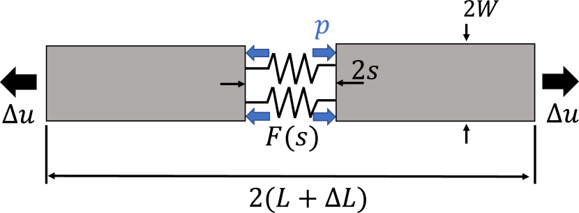
Figure 4: Uniaxial cohesive bar.

Table 1: Material properties for uniaxial bar

	Value	Unit
Young’s modulus (E)	4.0$\times 10^{5}$	MPa
Poisson’s ratio ($\nu$)	0.2	–
Nucleation energy ($\psi_{c}$)	5.6$\times 10^{-5}$	$\text{mJ mm}^{-3}$
Critical fracture energy ($G_{c}$)	0.12	$\text{mJ mm}^{-2}$
Residual stiffness ($\xi$)	1.0$\times 10^{-8}$	–

The problem consists of a bar under a displacement controlled load in a pressurized chamber, as shown in Figure 4. The bar is assumed to be made of a linear elastic material that undergoes cohesive fracture, with a traction-separation law $F(s)$.

The bar has an undeformed length $2L=400$ mm and width $2W=2$ mm. The material properties are given in Table 1. Symmetry boundary conditions are invoked to reduce the computational domain to the top-right quarter of the bar. The applied load is modeled as a displacement boundary condition on the right end of the domain. The mesh consists of rectangular elements of size $h$ along the length direction and size 1 mm in the width direction. The initial applied displacement increment is $\Delta u=5\times 10^{-4}$ mm. The displacement increment is adaptively refined when convergence is not obtained within a fixed set of iterations. A more detailed description of the adaptive stepping procedure is provided in [77, 78, 79].

Damage localization is triggered by introducing an small initial defect ($d=\mathcal{O}(\epsilon)$) on the left side of the domain. In what follows, results are reported using $\ell=L/20=10$ mm and $h=\ell/10=1$ mm. This choice of regularization length and mesh spacing was found to yield spatially-converged results. Different values of pressure, ranging from $0$ to $\sigma_{c}/3$ are considered.

The problem is simulated using discretized versions of both the LABEL:uvc and (LABEL:lvc) formulations.

For the indicator function $I(d)$, results are reported for: (1) $I(d)=d$, used for example in [8]; (2) $I(d)=d^{2}$, used in [12] and (3) $I(d)=2d-d^{2}$, used in [9]. The effective traction-separation laws extracted from the set of simulations are shown in Figure 5. To generate these curves, the traction is computed as the internal force measured in the center of the bar. The separation $s$ is the opening of the crack, calculated as $s=-\int\limits_{-\infty}^{\infty}\textbf{u}\cdot\nabla I(d)\text{dx}$ [8].

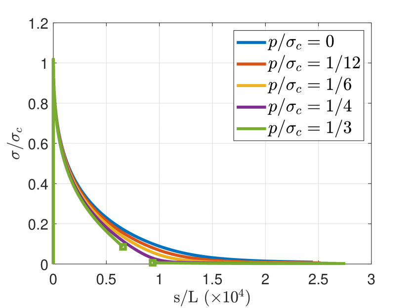
(a)

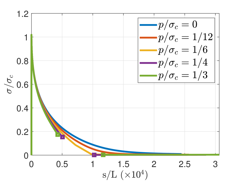
(b)

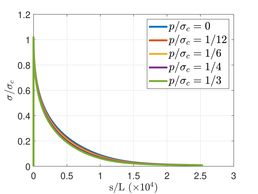
(c)

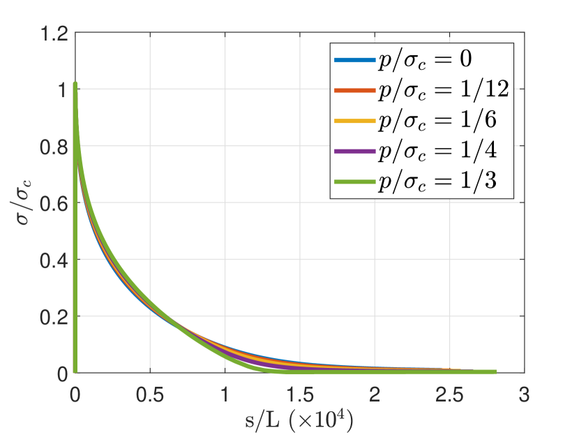
(d)

Figure 5: Traction-separation curves for pressurized uniaxial cohesive bar problem, obtained with various phase-field models: (a) (LABEL:lvc) with linear indicator function; (b) (LABEL:lvc) with quadratic indicator function; (c) (LABEL:lvc) with $2d-d^{2}$ indicator function; and (d) Proposed approach (LABEL:uvc) with linear indicator function.

The results for the various models are shown in Figure 5, with tractions and pressures normalized by the critical stress $\sigma_{c}$ from (79). As shown in Figure 5, the proposed model (LABEL:uvc) exhibits minimal sensitivity to the pressure magnitude in the traction-separation behavior. By contrast, with the (LABEL:lvc) formulation, only the case with $I(d)=2d-d^{2}$ exhibits comparable results. In the other two cases (Figures 5(a) and 5(b)), the apparent traction-separation law shows a spurious dependence to the applied pressure. This is evident in the variations in the results as well as the presence of jumps in the aperture at sufficiently high pressures. The latter occur due to an instability of the partially damaged solutions as $d$ approaches 1. More precisely, shortly after the damage at the center of the bar reaches $d\approx 0.8$, it jumps to $d=1$, which in turns lead to a jump in the aperture. This jump is indicated via the squares that appear on selected curves in Figures 5(a) and 5(b). The use of smaller displacement increments was not observed to significantly impact these results. By contrast, such instabilities were not observed for the simulations reported in Figures 5(c) and 5(d).

5.2 Crack nucleation from a pressurized hole

Consider a square plate of dimensions $L\times L$, with a circular hole in the center subjected to an internal pressure $p$, as shown in Figure 6(a). This problem is motivated by oil and gas wellbore systems. Far field stresses $\sigma_{V}$ and $\sigma_{H}$ are applied as tractions on the boundaries as shown. The pressure is increased until it reaches a “breakdown pressure” $p_{b}$. When that happens, cracks initiate in the direction parallel to the maximum in-situ stress. Assuming $\sigma_{H}>\sigma_{V}$, this is expected to occur along a horizontal axis passing through the center of the hole. In this work, the pressure in the hole is assumed to follow the crack faces as the fracture grows into the interior of the domain.

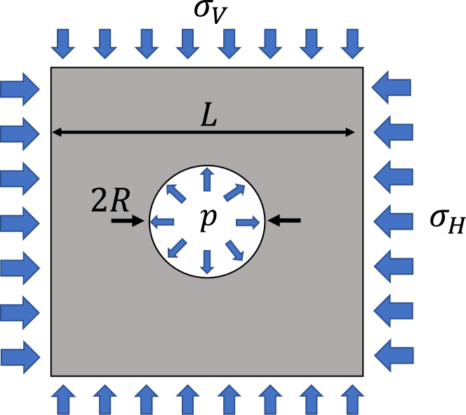
(a)

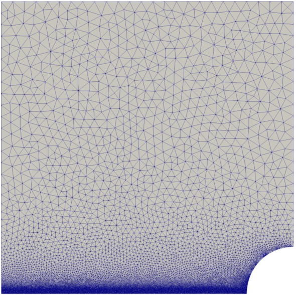
(b)

Figure 6: (a) Problem schematic; (b) Mesh used in the computations, exploiting symmetry.

Table 2: Material properties, geometric parameters and applied loads for crack initiation problem

	Value	Unit
Young’s modulus (E)	19.0$\times 10^{3}$	MPa
Poisson’s ratio ($\nu$)	0.2	–
Nucleation energy ($\psi_{c}$)	7.96$\times 10^{-4}$	$\text{mJ mm}^{-3}$
Critical fracture energy ($G_{c}$)	7.70$\times 10^{-2}$	$\text{mJ mm}^{-2}$
Cavity radius ($R$)	400	mm
Specimen length ($L$)	5.0$\times 10^{3}$	mm
Horizontal stress ($\sigma_{H}$)	5.0	MPa
Vertical stress ($\sigma_{V}$)	2.5	MPa

The material properties selected for this problem, along with the dimensions and loading parameters are listed in Table 2. The material properties are taken to be representative of a Bebertal sandstone, as inspired by the experiments of [80].

The symmetry of the problem is exploited to reduce the computational domain to the top-left quarter. An unstructured triangular mesh is used, with local refinement along the $x$-axis, as shown in Figure 6(b). The element size in the refined area is $10$mm, whereas the phase-field regularization length is $\ell=40$mm. For the results reported in this section, the phase-field model employs the cohesive formulation[52, 53] using the degradation function (41) and the spectral split of [61].

Intuitively, the magnitude of the pressure load required to initiate fracture in this problem is expected to be independent of whether or not the pressure follows the crack evolution. After initiation, the pressure effects become important and the fracture propagates unstably. Due to this unstable behavior, it is very difficult to numerically capture the crack path after the pressure $p_{b}$ is reached. In order to have a glimpse into what this path looks like, a viscous term $\eta\dot{d}$ is added to the phase-field equation, as in [61], with $\eta=10^{-3}\ \text{mJ}\cdot\text{mm}^{-3}\cdot$s.

It bears emphasis that the equations (9) and (11) indicate that, in the absence of any damage, the proposed model for pressurized cracks reduces to the standard phase-field fracture model for traction-free cracks. Therefore, one should expect the proposed model to capture fracture initiation properly in this scenario. On the other hand, for the (LABEL:lvc) formulation, this only occurs if the indicator function satisfies $I^{\prime}(0)=0$. Among the many works which use the (LABEL:lvc) formulation, only a few such as [12, 11] used an indicator function satisfying this condition. In [12], the authors were indeed able to predict fracture initiation from pressurized holes. To highlight the implications of having $I^{\prime}(0)\neq 0$ in the model (LABEL:lvc), the results for this problem will also be presented using the (LABEL:lvc) formulation with the indicator function $I(d)=d$.

The final damage patterns obtained using the (LABEL:uvc) formulation and the (LABEL:lvc) formulation are shown in Figure 7. With the (LABEL:uvc) formulation, damage localizes along the midplane when the hoop stress is approximately 85% of $\sigma_{c}$. This is not unexpected, as the expression (79) is based on a one-dimensional state of stress and strain which differs significantly from the state near the corner of the hole. The same comparison is not performed for the simulation using the model (LABEL:lvc), since damage forms only on the boundary in the first steps leading to spurious rigid body motion.

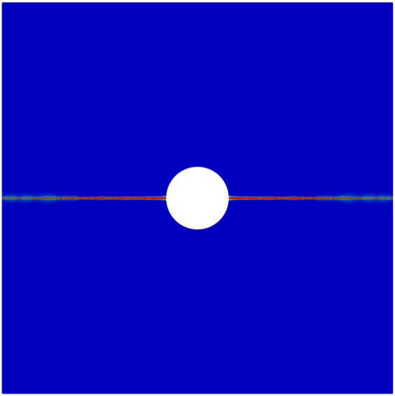
(a)

(b)

Figure 7: (a) Final crack pattern using proposed model; (b) Damage field using the model from [8].

The main takeaway is that the proposed model (LABEL:uvc) allows one to study crack nucleation and subsequent propagation under a pressure load, whereas formulation (LABEL:lvc) leads to spurious damage formation if $I^{\prime}(0)\neq 0$. The presence of the term $p\nabla\cdot\textbf{u}I^{\prime}(d)$ in the damage equation (19) drives crack formation in areas which are not stressed. For this specific problem, this issue can be circumvented using for example $I(d)=d^{2}$, as shown in [12], but this option introduces a spurious dependence of the cohesive response of the material on the applied pressure, as indicated in the last section (Figure 5(b)).

5.3 Stable propagation of a pre-existing crack

Consider a strip of material with a pressurized crack, as shown in Figure 8(a). The rectangular strip has a width $W$, height $H$ and a crack with initial size $a$ (values provided in Table 3), and is loaded by the “surfing” boundary condition $\widetilde{U_{y}}(x,y,t)$ on its top and bottom surfaces [57]. The boundary condition is given by

$$\widetilde{U_{y}}(x,y,t)=U_{y}(x-Vt,y),$$ (80)

where

$$U_{y}(x,y)=\hat{U}_{y}(r,\theta)=\dfrac{\sqrt{G_{c}E^{\prime}}}{2\mu}\sqrt{\dfrac{r}{2\pi}}(\kappa-\cos\theta)\sin\dfrac{\theta}{2},$$ (81)

and where $r$ and $\theta$ are polar coordinates with respect to the origin, taken to be the midpoint of the left edge of the domain. The constant $V>0$ is the target crack speed, prescribed by moving the boundary condition following (80). The Kolosov constant is defined as $\kappa=3-4\nu$ in plane strain and the shear modulus $\mu=E/(2+2\nu)$. The pressure $p$ applied to the crack faces as the crack evolves is given by

$$p=\dfrac{1}{2}\sqrt{\dfrac{G_{c}E^{\prime}}{\pi a}},$$ (82)

in which $a$ denotes the initial crack length. This value corresponds to half the critical pressure for an infinite plate with a pressurized crack of size $a$. This magnitude ensures that the applied pressure is considerably large, but not so large as to drive the problem beyond the stable propagation regime.

To calculate the energy release rate, the domain form of the J-integral (44) developed in Section 3 is used. The function $q$ is constructed by taking advantage of the finite element interpolation. In essence, the domain for the J-integral is taken to be a single rectangular region of dimensions $a\times H/2$, centered on the initial crack tip. The value of $q$ for all nodes outside of this region is set to $0$, while $q=1$ for all nodes inside. Using the finite element interpolation, this gives rise to a $q$ function whose value changes continuously from $0$ to $1$ on the elements cut by the rectangular path. This function is illustrated in Figure 8(b).

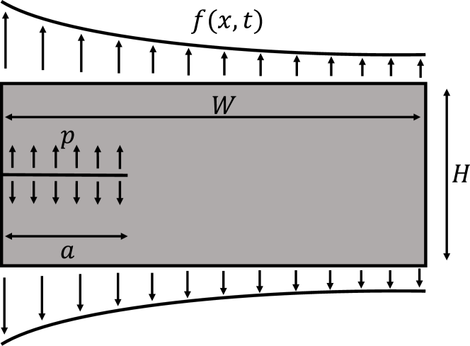
(a)

(b)

Figure 8: (a) Geometry and boundary conditions for pressurized crack propagation problem; (b) J-Integral domain function $q$.

Table 3: Parameters used for pressurized crack propagation problem

	Value	Unit
Young’s modulus (E)	3.0$\times 10^{4}$	MPa
Poisson’s ratio ($\nu$)	0.2	–
Critical fracture energy ($G_{c}$)	0.12	$\text{mJ mm}^{-2}$
Initial crack length ($a$)	1.6	m
Specimen width ($W$)	8.0	m
Specimen height ($H$)	4.0	m
Target crack speed ($V$)	0.4	m/s

In order to verify that Griffith’s law is approached as $\ell\rightarrow 0$, simulations are performed for this problem using a sequence of decreasing regularization lengths, ranging from $\ell=a/20$ to $\ell=a/160$. The mesh is locally refined along the $x$-axis, where the element size is set to $h=\ell/4$. The symmetry of the problem is exploited and only the response in the top half of the domain is simulated.

In terms of constitutive choices of the phase-field model, the AT-1 formulation is employed without any decomposition of the strain.

As in the previous examples, this problem is analyzed using the formulations (LABEL:lvc) and (LABEL:uvc), and the following choices of indicator function $I(d)$:

• $I(d)=d$

• $I(d)=d^{2}$

• $I(d)=2d-d^{2}$

To evaluate how well the models approach Griffith’s law, the ratio between the energy release rate measured by the J-Integral and the effective critical fracture energy $G^{eff}_{c}=(1+2h/c_{0}\ell)G_{c}$ is plotted in Figures 9 and 10. In all figures, the time is scaled by a characteristic time $\tau$, defined as $\tau=a/V$. The results using the traditional (LABEL:lvc) formulation are presented in Figure 9. They indicate convergence towards $J/G^{eff}_{c}$ = 1 as the regularization length is reduced, especially when the indicator function $I(d)=d$ is used. This is expected given the results obtained in [8]. Nevertheless, these results serve to verify the implementation of the J-Integral presented in Section 3. They also provide an estimate for how small the regularization length has to be in order to achieve a certain level of accuracy with these types of phase-field models.

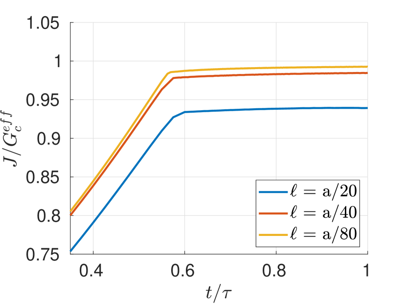
(a)

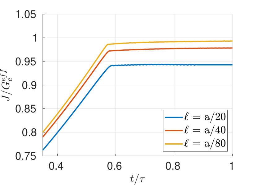
(b)

(c)

Figure 9: Reference results with the LABEL:lvc formulation. Curves with $\ell=a/160$ are not shown, as they are almost identical to the ones with $\ell=a/80$. (a) $I(d)=d$; (b) $I(d)=d^{2}$; (c) $I(d)=2d-d^{2}$

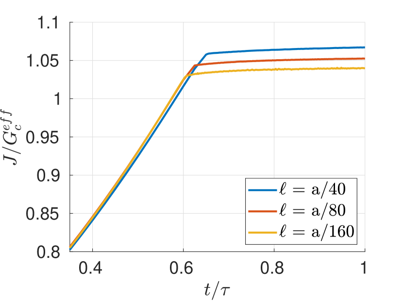
(a)

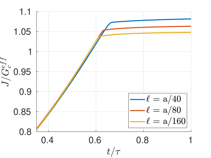
(b)

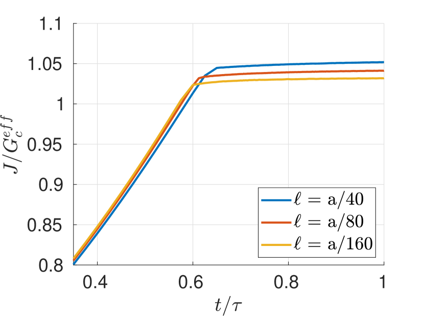
(c)

Figure 10: Results with the proposed formulation (LABEL:uvc) (a) $I(d)=d$; (b) $I(d)=d^{2}$; (c) $I(d)=2d-d^{2}$

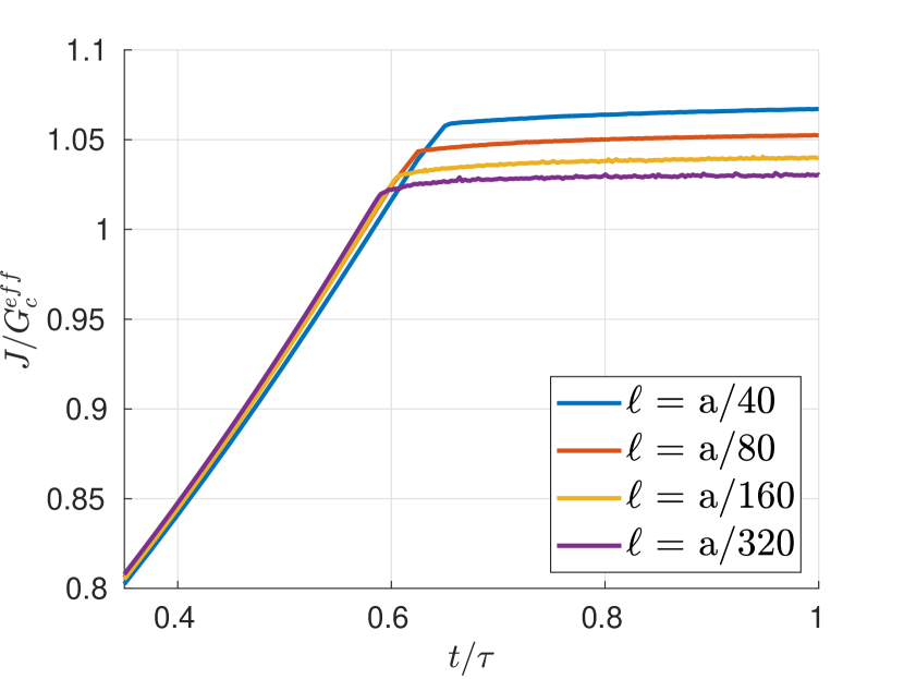
Figure 11: Convergence of the proposed formulation with $I(d)=d$.

$\ell/a$	Error	$\text{Error}_{k+1}/\text{Error}_{k}$
1/40	0.067	–
1/80	0.052	0.78
1/160	0.040	0.77
1/320	0.031	0.77

Table 4: Absolute error in $J$ vs. $G_{c}^{eff}$ for the pressurized crack propagation problem, as a function of regularization length.

For the case of proposed formulation (LABEL:uvc), the results shown in Figure 10 indicate a slower convergence towards a $J/G^{eff}_{c}=1$ response. In contrast with the (LABEL:lvc) formulation, the curves converge from above, and therefore, the fracture toughness is slightly overestimated when larger regularization lengths are used. Nevertheless, they all seem to approach a Griffith-like response in the limit $\ell\rightarrow 0$. In Figure 11, an even finer result, using (LABEL:uvc) with $I(d)=d$ and $\ell=a/320$ is added, to ensure that the convergence rates indicated in Figure 10 persist. In Table 4, the relative errors are provided, indicating a convergence rate of approximately $0.4$ with respect to $\ell$.

One potential explanation for the slower convergence rate is related to the different assumptions regarding the trial cracks, as discussed in Section 2. Although the different assumptions converge to the same propagation rule in the limit of an infinitesimal crack increment, in the discretized case, the minimal crack increment is finite and related to the mesh spacing $h$ and regularization length $\ell$. In this case, a slightly different propagation behavior, resulting in slower convergence rates towards $J/G^{eff}_{c}=1$ is not surprising.

6 Concluding Remarks

This manuscript examines various models for phase-field fracture incorporating pressure loads on diffuse crack faces. This includes the analysis of a new formulation that can be obtained by considering the presence of the pressure load in the virtual extension of a crack, or alternatively through a careful accounting in the minimization procedure. The new formulation is referred to as the “unloaded virtual crack formulation”(LABEL:uvc). In order to verify the accuracy of the various models for propagating cracks, a new form of the J-Integral for pressurized cracks in the phase-field context is derived.

The (LABEL:uvc) formulation proposed herein allows for a unified treatment of crack nucleation and propagation in scenarios involving either brittle or cohesive fracture, and provides for better accuracy in some problems compared to existing formulations of the (LABEL:lvc) type. As it allows for the use of the same governing equation for the damage parameter, its computational implementation within existing phase-field solvers is also simpler. In future work, its applicability to problems involving plastic deformation and strength-based fracture nucleation will be studied. In addition to that, modifications to accelerate the convergence of the model with respect to the phase-field parameter $\ell$ will also be considered.

7 Acknowledgments

The partial support of A. Costa and J.E. Dolbow by the National Science Foundation, through grant CMMI-1933367 to Duke University, is gratefully acknowledged. T. Hu gratefully acknowledges the support of Argonne National Laboratory. Argonne National Laboratory is managed and operated by UChicago Argonne LLC. for the U.S. Department of Energy under Contract No. DE-AC02-06CH11357.

Appendix A Equivalence to SIF condition

In this appendix, the energy release rate for a single, straight crack under an arbitrary pressure load $p(x)$ is computed, assuming that infinitesimal crack increments are traction free, as shown in Figure 2(a). Griffith’s criteria states that propagation should happen whenever this energy release rate, which will be denoted by $G$, reaches $G_{c}$. This will give rise to a condition for propagation based on the pressure distribution $p(x)$, the crack size $a$ and Young’s modulus $E^{\prime}$. The purpose of the following derivation is to demonstrate that this condition is equivalent to the stress intensity factor criteria [81].

Initially, consider the Sneddon-Lowengrub solution for the aperture of a pressure loaded crack in an infinite plate, under plane strain conditions,

$$w(x)=\dfrac{4a}{\pi E^{\prime}}\int^{1}_{0}p(sa)Z(x/a,s)\text{d}s$$ (83)

where

$$Z(r,s)=\log\left|\dfrac{\sqrt{1-r^{2}}+\sqrt{1-s^{2}}}{\sqrt{1-r^{2}}-\sqrt{1-s^{2}}}\right|$$ (84)

is a convolution kernel. The work done by the pressure load is then,

$$W_{p}=\int_{-a}^{a}pw\text{d}x=\int_{-a}^{a}p(y)\dfrac{4a}{\pi E^{\prime}}\int^{1}_{0}p(sa)Z(x/a,s)\text{d}s\text{d}y.$$ (85)

Clayperon’s theorem [82] states that the potential energy is negative half of the work exerted in the boundary, which, in this case is only $W_{p}$. Hence

$$U=-\dfrac{1}{2}W_{p}=-\dfrac{1}{2}\int_{-a}^{a}pw\text{d}x\\ =-\dfrac{4a^{2}}{\pi E^{\prime}}\int_{0}^{1}p(ar)\int^{1}_{0}p(sa)Z(r,s)\text{d}s\text{d}r.$$ (86)

Let’s write the energy release rate, assuming that the pressure field doesn’t vary as the crack advances by a small amount $\text{d}a$. That is,

$$p^{a+\text{d}a}(x)=\begin{cases}p^{a}(x),&\text{if}\ x\leq a\\ 0,&\text{if}\ a\leq x\leq a+\text{d}a\end{cases}$$ (87)

$$dU=U(a+\text{d}a,p^{a+\text{d}a})-U(a+\text{d}a,p^{a}),$$ (88)

$$dU=\\ -\dfrac{4}{\pi E^{\prime}}\int_{0}^{a+\text{d}a}p^{a+\text{d}a}(x)\int_{0}^{a+\text{d}a}p^{a+\text{d}a}(y)Z(\frac{x}{a+\text{d}a},\frac{y}{a+\text{d}a})\text{d}y\text{d}x\\ +\dfrac{4}{\pi E^{\prime}}\int_{0}^{a}p^{a}(x)\int_{0}^{a}p^{a}(y)Z(x/a,y/a)\text{d}y\text{d}x.$$ (89)

Using the definition of $p^{a+\text{d}a}$ given above,

$$dU=-\frac{4}{\pi E^{\prime}}\times\\ \int_{0}^{a}p^{a}(x)\int_{0}^{a}p^{a}(y)\left(Z(\frac{x}{a+\text{d}a},\frac{y}{a+\text{d}a})-Z(x/a,y/a)\right)\text{d}y\text{d}x.$$

By symmetry, both tips of the crack propagate with the same energy release rate, so, one can write,

$$2G=-\dfrac{dU}{\text{d}a}=\dfrac{4}{\pi E^{\prime}}\times\dfrac{1}{\text{d}a}\times\\ \int_{0}^{a}p^{a}(x)\int_{0}^{a}p^{a}(y)\left(Z(\frac{x}{a+\text{d}a},\frac{y}{a+\text{d}a})-Z(x/a,y/a)\right)\text{d}y\text{d}x.$$

The term between parenthesis can be re-written as,

$$Z(\frac{x}{a+\text{d}a},\frac{y}{a+\text{d}a})-Z(x/a,y/a)=\\ \log\left|\dfrac{\sqrt{(a+\text{d}a)^{2}-x^{2}}+\sqrt{(a+\text{d}a)^{2}-y^{2}}}{\sqrt{(a+\text{d}a)^{2}-x^{2}}-\sqrt{(a+\text{d}a)^{2}-y^{2}}}\right|\\ -\log\left|\dfrac{\sqrt{a^{2}-x^{2}}+\sqrt{a^{2}-y^{2}}}{\sqrt{a^{2}-x^{2}}-\sqrt{a^{2}-y^{2}}}\right|\\ =\log\left|\dfrac{\sqrt{(a+\text{d}a)^{2}-x^{2}}+\sqrt{(a+\text{d}a)^{2}-y^{2}}}{\sqrt{a^{2}-x^{2}}+\sqrt{a^{2}-y^{2}}}\right|\\ -\log\left|\dfrac{\sqrt{(a+\text{d}a)^{2}-x^{2}}-\sqrt{(a+\text{d}a)^{2}-y^{2}}}{\sqrt{a^{2}-x^{2}}-\sqrt{a^{2}-y^{2}}}\right|.$$ (90)

The second term contains a singularity, which can be removed if one re-writes it as,

$$\log\left|\dfrac{\sqrt{(a+\text{d}a)^{2}-x^{2}}-\sqrt{(a+\text{d}a)^{2}-y^{2}}}{\sqrt{a^{2}-x^{2}}-\sqrt{a^{2}-y^{2}}}\right|=\\ \log\biggl{|}\dfrac{\sqrt{(a+\text{d}a)^{2}-x^{2}}-\sqrt{(a+\text{d}a)^{2}-y^{2}}}{\sqrt{a^{2}-x^{2}}-\sqrt{a^{2}-y^{2}}}\\ \times\dfrac{\sqrt{(a+\text{d}a)^{2}-x^{2}}+\sqrt{(a+\text{d}a)^{2}-y^{2}}}{\sqrt{a^{2}-x^{2}}+\sqrt{a^{2}-y^{2}}}\\ \times\dfrac{\sqrt{a^{2}-x^{2}}+\sqrt{a^{2}-y^{2}}}{\sqrt{(a+\text{d}a)^{2}-x^{2}}+\sqrt{(a+\text{d}a)^{2}-y^{2}}}\biggr{|}\\ =\log\biggl{|}\dfrac{(a+\text{d}a)^{2}-x^{2}-(a+\text{d}a)^{2}+y^{2}}{a^{2}-x^{2}-a^{2}+y^{2}}\\ \times\dfrac{\sqrt{a^{2}-x^{2}}+\sqrt{a^{2}-y^{2}}}{\sqrt{(a+\text{d}a)^{2}-x^{2}}+\sqrt{(a+\text{d}a)^{2}-y^{2}}}\biggr{|}\\ =-\log\left|\dfrac{\sqrt{(a+\text{d}a)^{2}-x^{2}}+\sqrt{(a+\text{d}a)^{2}-y^{2}}}{\sqrt{a^{2}-x^{2}}+\sqrt{a^{2}-y^{2}}}\right|.$$ (91)

This expression can be plugged back into (90) to obtain,

$$Z(\frac{x}{a+\text{d}a},\frac{y}{a+\text{d}a})-Z(x/a,y/a)=\\ \log\left|\dfrac{\sqrt{(a+\text{d}a)^{2}-x^{2}}+\sqrt{(a+\text{d}a)^{2}-y^{2}}}{\sqrt{(a+\text{d}a)^{2}-x^{2}}-\sqrt{(a+\text{d}a)^{2}-y^{2}}}\right|\\ -\log\left|\dfrac{\sqrt{a^{2}-x^{2}}+\sqrt{a^{2}-y^{2}}}{\sqrt{a^{2}-x^{2}}-\sqrt{a^{2}-y^{2}}}\right|\\ =2\log\left|\dfrac{\sqrt{(a+\text{d}a)^{2}-x^{2}}+\sqrt{(a+\text{d}a)^{2}-y^{2}}}{\sqrt{a^{2}-x^{2}}+\sqrt{a^{2}-y^{2}}}\right|.$$ (92)

Hence,

$$\dfrac{1}{\text{d}a}\left(Z(\frac{x}{a+\text{d}a},\frac{y}{a+\text{d}a})-Z(x/a,y/a)\right)\\ =\dfrac{2}{\text{d}a}\log\left|\dfrac{\sqrt{(a+\text{d}a)^{2}-x^{2}}+\sqrt{(a+\text{d}a)^{2}-y^{2}}}{\sqrt{a^{2}-x^{2}}+\sqrt{a^{2}-y^{2}}}\right|.$$ (93)

Now, the terms in the numerator can be expanded with a Taylor series,

$$\sqrt{(a+\text{d}a)^{2}-x^{2}}=\sqrt{a^{2}-x^{2}}+\dfrac{a}{\sqrt{a^{2}-x^{2}}}\text{d}a+O(\text{d}a^{2}),$$ (94)

leading to,

$$\dfrac{1}{\text{d}a}\left(Z(\frac{x}{a+\text{d}a},\frac{y}{a+\text{d}a})-Z(x/a,y/a)\right)=\\ \dfrac{2}{\text{d}a}\log\Biggl{|}\dfrac{\sqrt{a^{2}-x^{2}}+\dfrac{a}{\sqrt{a^{2}-x^{2}}}\text{d}a+O(\text{d}a^{2})}{\sqrt{a^{2}-x^{2}}+\sqrt{a^{2}-y^{2}}}\\ +\dfrac{\sqrt{a^{2}-y^{2}}+\dfrac{a}{\sqrt{a^{2}-y^{2}}}\text{d}a+O(\text{d}a^{2})}{\sqrt{a^{2}-x^{2}}+\sqrt{a^{2}-y^{2}}}\Biggr{|},$$ (95)

which, after using a Taylor expansion, simplifies to,

$$\dfrac{1}{\text{d}a}\left(Z(\frac{x}{a+\text{d}a},\frac{y}{a+\text{d}a})-Z(x/a,y/a)\right)\\ =\dfrac{2a}{\sqrt{a^{2}-x^{2}}\sqrt{a^{2}-y^{2}}}+O(\text{d}a).$$ (96)

Now, we can finally go back to the energy release rate,

$$2G=-\dfrac{dU}{\text{d}a}\\ =\dfrac{4}{\pi E^{\prime}}\int_{0}^{a}p^{a}(x)\int_{0}^{a}p^{a}(y)\dfrac{2a}{\sqrt{a^{2}-x^{2}}\sqrt{a^{2}-y^{2}}}\text{d}y\text{d}x\\ =\dfrac{8a}{\pi E^{\prime}}\int_{0}^{1}\dfrac{p^{a}(ar)}{\sqrt{1-r^{2}}}\int_{0}^{1}\dfrac{p^{a}(as)}{\sqrt{1-s^{2}}}\text{d}s\text{d}r\\ =\dfrac{8a}{\pi E^{\prime}}\left(\int_{0}^{1}\dfrac{p^{a}(as)}{\sqrt{1-s^{2}}}\text{d}s\right)^{2}.$$ (97)

From [83], the stress intensity factor under these same conditions is,

$$K_{I}=2\sqrt{\dfrac{a}{\pi}}\left(\int_{0}^{1}\dfrac{p^{a}(as)}{\sqrt{1-s^{2}}}\text{d}s\right)$$ (98)

From a simple inspection, one can see that $G=K_{I}^{2}/E^{\prime}$, which guarantees the equivalence of the energy release rate criteria under the assumption in Figure 2(a) and the stress intensity factor condition. If instead, one assumes that the pressure load in the vicinity of a propagating crack behaves as in Figure 2(b), this equivalence between the energetic criteria and the stress intensity factor may be violated.

References

- [1] Q. Li, H. Xing, J. Liu, X. Liu, A review on hydraulic fracturing of unconventional reservoir, Petroleum 1 (1) (2015) 8–15.
- [2] R. Mair, M. Bickle, D. Goodman, B. Koppelman, J. Roberts, R. Selley, Z. Shipton, H. Thomas, A. Walker, E. Woods, et al., Shale gas extraction in the UK: a review of hydraulic fracturing, technical report (2012).
- [3] A. Shinmura, V. E. Saouma, Fluid fracture interaction in pressurized reinforced concrete vessels, Materials and Structures 30 (2) (1997) 72–80.
- [4] Y. Wang, J. Jia, Experimental study on the influence of hydraulic fracturing on high concrete gravity dams, Engineering Structures 132 (2017) 508–517.
- [5] N. Capps, C. Jensen, F. Cappia, J. Harp, K. Terrani, N. Woolstenhulme, D. Wachs, A critical review of high burnup fuel fragmentation, relocation, and dispersal under loss-of-coolant accident conditions, Journal of Nuclear Materials 546 (2021) 152750.
- [6] J. Turnbull, S. Yagnik, M. Hirai, D. Staicu, C. Walker, An assessment of the fuel pulverization threshold during LOCA-type temperature transients, Nuclear Science and Engineering 179 (4) (2015) 477–485.
- [7] B. Bourdin, G. A. Francfort, J.-J. Marigo, Numerical experiments in revisited brittle fracture, Journal of the Mechanics and Physics of Solids 48 (4) (2000) 797–826.
- [8] B. Bourdin, C. P. Chukwudozie, K. Yoshioka, et al., A variational approach to the numerical simulation of hydraulic fracturing, in: SPE Annual Technical Conference and Exhibition, Society of Petroleum Engineers, 2012.
- [9] M. F. Wheeler, T. Wick, W. Wollner, An augmented-lagrangian method for the phase-field approach for pressurized fractures, Computer Methods in Applied Mechanics and Engineering 271 (2014) 69–85.
- [10] A. Mikelić, M. F. Wheeler, T. Wick, A quasi-static phase-field approach to pressurized fractures, Nonlinearity 28 (5) (2015) 1371.
- [11] C. Peco, W. Chen, Y. Liu, M. Bandi, J. E. Dolbow, E. Fried, Influence of surface tension in the surfactant-driven fracture of closely-packed particulate monolayers, Soft Matter 13 (35) (2017) 5832–5841.
- [12] W. Jiang, T. Hu, L. K. Aagesen, S. Biswas, K. A. Gamble, A phase-field model of quasi-brittle fracture for pressurized cracks: Application to UO2 high-burnup microstructure fragmentation, Theoretical and Applied Fracture Mechanics 119 (2022) 103348.
- [13] T. Hu, A variational framework for phase-field fracture modeling with applications to fragmentation, desiccation, ductile failure, and spallation, Ph.D. thesis, Duke University (2021).
- [14] A. Karma, D. A. Kessler, H. Levine, Phase-field model of mode iii dynamic fracture, Physical Review Letters 87 (4) (2001) 045501.
- [15] G. A. Francfort, J.-J. Marigo, Revisiting brittle fracture as an energy minimization problem, Journal of the Mechanics and Physics of Solids 46 (8) (1998) 1319–1342.
- [16] L. Ambrosio, V. M. Tortorelli, Approximation of functional depending on jumps by elliptic functional via t-convergence, Communications on Pure and Applied Mathematics 43 (8) (1990) 999–1036.
- [17] R. Alessi, J.-J. Marigo, S. Vidoli, Gradient damage models coupled with plasticity and nucleation of cohesive cracks, Archive for Rational Mechanics and Analysis 214 (2) (2014) 575–615.
- [18] M. Ambati, T. Gerasimov, L. De Lorenzis, Phase-field modeling of ductile fracture, Computational Mechanics 55 (5) (2015) 1017–1040.
- [19] C. Miehe, S. Mauthe, Phase field modeling of fracture in multi-physics problems. part iii. crack driving forces in hydro-poro-elasticity and hydraulic fracturing of fluid-saturated porous media, Computer Methods in Applied Mechanics and Engineering 304 (2016) 619–655.
- [20] M. J. Borden, T. J. Hughes, C. M. Landis, A. Anvari, I. J. Lee, A phase-field formulation for fracture in ductile materials: Finite deformation balance law derivation, plastic degradation, and stress triaxiality effects, Computer Methods in Applied Mechanics and Engineering 312 (2016) 130–166.
- [21] T. Hu, B. Talamini, A. J. Stershic, M. R. Tupek, J. E. Dolbow, A variational phase-field model for ductile fracture with coalescence dissipation, Computational Mechanics 68 (2) (2021) 311–335.
- [22] Z. A. Wilson, C. M. Landis, Phase-field modeling of hydraulic fracture, Journal of the Mechanics and Physics of Solids 96 (2016) 264–290.
- [23] C. Chukwudozie, B. Bourdin, K. Yoshioka, A variational phase-field model for hydraulic fracturing in porous media, Computer Methods in Applied Mechanics and Engineering 347 (2019) 957–982.
- [24] A. Mikelić, M. F. Wheeler, T. Wick, Phase-field modeling of a fluid-driven fracture in a poroelastic medium, Computational Geosciences 19 (6) (2015) 1171–1195.
- [25] D. Santillán, R. Juanes, L. Cueto-Felgueroso, Phase field model of hydraulic fracturing in poroelastic media: Fracture propagation, arrest, and branching under fluid injection and extraction, Journal of Geophysical Research: Solid Earth 123 (3) (2018) 2127–2155.
- [26] C. Maurini, B. Bourdin, G. Gauthier, V. Lazarus, Crack patterns obtained by unidirectional drying of a colloidal suspension in a capillary tube: experiments and numerical simulations using a two-dimensional variational approach, International Journal of Fracture 184 (1-2) (2013) 75–91.
- [27] Y. Heider, W. Sun, A phase field framework for capillary-induced fracture in unsaturated porous media: Drying-induced vs. hydraulic cracking, Computer Methods in Applied Mechanics and Engineering 359 (2020) 112647.
- [28] T. Cajuhi, L. Sanavia, L. De Lorenzis, Phase-field modeling of fracture in variably saturated porous media, Computational Mechanics 61 (3) (2018) 299–318.
- [29] H. Tianchen, J. Guilleminot, J. Dolbow, A phase-field model of fracture with frictionless contact and random fracture properties: Application to thin-film fracture and soil desiccation, Computer Methods in Applied Mechanics and Engineering 368 (2020).
- [30] B. Bourdin, C. J. Larsen, C. L. Richardson, A time-discrete model for dynamic fracture based on crack regularization, International Journal of Fracture 168 (2) (2011) 133–143.
- [31] M. J. Borden, C. V. Verhoosel, M. A. Scott, T. J. Hughes, C. M. Landis, A phase-field description of dynamic brittle fracture, Computer Methods in Applied Mechanics and Engineering 217 (2012) 77–95.
- [32] M. Hofacker, C. Miehe, A phase field model of dynamic fracture: Robust field updates for the analysis of complex crack patterns, International Journal for Numerical Methods in Engineering 93 (3) (2013) 276–301.
- [33] A. Schlüter, A. Willenbücher, C. Kuhn, R. Müller, Phase field approximation of dynamic brittle fracture, Computational Mechanics 54 (5) (2014) 1141–1161.
- [34] T. Li, J.-J. Marigo, D. Guilbaud, S. Potapov, Gradient damage modeling of brittle fracture in an explicit dynamics context, International Journal for Numerical Methods in Engineering 108 (11) (2016) 1381–1405.
- [35] D. Kamensky, G. Moutsanidis, Y. Bazilevs, Hyperbolic phase field modeling of brittle fracture: Part i—theory and simulations, Journal of the Mechanics and Physics of Solids 121 (2018) 81–98.
- [36] G. Moutsanidis, D. Kamensky, J. Chen, Y. Bazilevs, Hyperbolic phase field modeling of brittle fracture: Part ii—immersed iga–rkpm coupling for air-blast–structure interaction, Journal of the Mechanics and Physics of Solids 121 (2018) 114–132.
- [37] C. Wu, J. Fang, Z. Zhang, A. Entezari, G. Sun, M. V. Swain, Q. Li, Fracture modeling of brittle biomaterials by the phase-field method, Engineering Fracture Mechanics 224 (2020) 106752.
- [38] A. Raina, C. Miehe, A phase-field model for fracture in biological tissues, Biomechanics and modeling in mechanobiology 15 (3) (2016) 479–496.
- [39] S. Nagaraja, K. Leichsenring, M. Ambati, L. De Lorenzis, M. Böl, On a phase-field approach to model fracture of small intestine walls, Acta Biomaterialia 130 (2021) 317–331.
- [40] O. Gültekin, H. Dal, G. A. Holzapfel, A phase-field approach to model fracture of arterial walls: theory and finite element analysis, Computer Methods in Applied Mechanics and Engineering 312 (2016) 542–566.
- [41] O. Gültekin, H. Dal, G. A. Holzapfel, Numerical aspects of anisotropic failure in soft biological tissues favor energy-based criteria: A rate-dependent anisotropic crack phase-field model, Computer Methods in Applied Mechanics and Engineering 331 (2018) 23–52.
- [42] M. Ambati, T. Gerasimov, L. De Lorenzis, A review on phase-field models of brittle fracture and a new fast hybrid formulation, Computational Mechanics 55 (2) (2015) 383–405.
- [43] J.-Y. Wu, V. P. Nguyen, C. T. Nguyen, D. Sutula, S. Sinaie, S. P. Bordas, Phase-field modeling of fracture, in: Advances in Applied Mechanics, Vol. 53, Elsevier, 2020, pp. 1–183.
- [44] G. Francfort, Variational fracture: twenty years after, International Journal of Fracture (2021) 1–11.
- [45] E. Tanné, B. Bourdin, K. Yoshioka, On the loss of symmetry in toughness dominated hydraulic fractures, International Journal of Fracture 237 (1-2) (2022) 189–202.
- [46] P. Zulian, A. Kopaničáková, M. G. C. Nestola, A. Fink, N. A. Fadel, J. VandeVondele, R. Krause, Large scale simulation of pressure induced phase-field fracture propagation using utopia, CCF transactions on high performance computing 3 (4) (2021) 407–426.
- [47] K. Yoshioka, F. Parisio, D. Naumov, R. Lu, O. Kolditz, T. Nagel, Comparative verification of discrete and smeared numerical approaches for the simulation of hydraulic fracturing, GEM-International Journal on Geomathematics 10 (1) (2019) 13.
- [48] K. Yoshioka, D. Naumov, O. Kolditz, On crack opening computation in variational phase-field models for fracture, Computer Methods in Applied Mechanics and Engineering 369 (2020) 113210.
- [49] Y. Heider, B. Markert, A phase-field modeling approach of hydraulic fracture in saturated porous media, Mechanics Research Communications 80 (2017) 38–46.
- [50] H. Li, H. Lei, Z. Yang, J. Wu, X. Zhang, S. Li, A hydro-mechanical-damage fully coupled cohesive phase field model for complicated fracking simulations in poroelastic media, Computer Methods in Applied Mechanics and Engineering 399 (2022) 115451.
- [51] Y. Heider, A review on phase-field modeling of hydraulic fracturing, Engineering Fracture Mechanics 253 (2021) 107881.
- [52] E. Lorentz, S. Cuvilliez, K. Kazymyrenko, Convergence of a gradient damage model toward a cohesive zone model, Comptes Rendus Mécanique 339 (1) (2011) 20–26.
- [53] R. J. Geelen, Y. Liu, T. Hu, M. R. Tupek, J. E. Dolbow, A phase-field formulation for dynamic cohesive fracture, Computer Methods in Applied Mechanics and Engineering 348 (2019) 680–711.
- [54] J.-Y. Wu, A unified phase-field theory for the mechanics of damage and quasi-brittle failure, Journal of the Mechanics and Physics of Solids 103 (2017) 72–99.
- [55] P. Sicsic, J.-J. Marigo, From gradient damage laws to griffith’s theory of crack propagation, Journal of Elasticity 113 (1) (2013) 55–74.
- [56] R. Ballarini, G. Royer-Carfagni, Closed-path j-integral analysis of bridged and phase-field cracks, Journal of Applied Mechanics 83 (6) (2016).
- [57] M. Hossain, C.-J. Hsueh, B. Bourdin, K. Bhattacharya, Effective toughness of heterogeneous media, Journal of the Mechanics and Physics of Solids 71 (2014) 15–32.
- [58] F. Z. Li, C. F. Shih, A. Needleman, A comparison of methods for calculating energy release rates, Engineering Fracture Mechanics 21 (2) (1985) 405–421.
- [59] C. Shih, B. Moran, T. Nakamura, Energy release rate along a three-dimensional crack front in a thermally stressed body, International Journal of Fracture 30 (2) (1986) 79–102.
- [60] H. Amor, J.-J. Marigo, C. Maurini, Regularized formulation of the variational brittle fracture with unilateral contact: Numerical experiments, Journal of the Mechanics and Physics of Solids 57 (8) (2009) 1209–1229.
- [61] C. Miehe, M. Hofacker, F. Welschinger, A phase field model for rate-independent crack propagation: Robust algorithmic implementation based on operator splits, Computer Methods in Applied Mechanics and Engineering 199 (45-48) (2010) 2765–2778.
- [62] E. Detournay, Mechanics of hydraulic fractures, Annual Review of Fluid Mechanics 48 (2016) 311–339.
- [63] D. Garagash, E. Detournay, The tip region of a fluid-driven fracture in an elastic medium, Journal of Applied Mechanics 67 (1) (2000) 183–192.
- [64] E. Detournay, Propagation regimes of fluid-driven fractures in impermeable rocks, International Journal of Geomechanics 4 (1) (2004) 35–45.
- [65] D. I. Garagash, E. Detournay, Plane-strain propagation of a fluid-driven fracture: small toughness solution, Journal of Applied Mechanics 72 (6) (2005) 916–928.
- [66] A. P. Bunger, E. Detournay, D. I. Garagash, Toughness-dominated hydraulic fracture with leak-off, International Journal of Fracture 134 (2) (2005) 175–190.
- [67] W. Jiang, T. Hu, L. K. Aagesen, Y. Zhang, Three-dimensional phase-field modeling of porosity dependent intergranular fracture in UO2, Computational Materials Science 171 (2020) 109269.
- [68] E. Lorentz, V. Godard, Gradient damage models: Toward full-scale computations, Computer Methods in Applied Mechanics and Engineering 200 (21-22) (2011) 1927–1944.
- [69] J. R. Rice, et al., Mathematical analysis in the mechanics of fracture, Fracture: an advanced treatise 2 (1968) 191–311.
- [70] J. R. Rice, A path independent integral and the approximate analysis of strain concentration by notches and cracks, Journal of Applied Mechanics 35 (2) (1968) 379–386.
- [71] A. Karlsson, J. Backlund, J-integral at loaded crack surfaces, International Journal of Fracture 14 (1978) 311–318.
- [72] W. Karush, Minima of functions of several variables with inequalities as side constraints, M. Sc. Dissertation. Dept. of Mathematics, Univ. of Chicago (1939).
- [73] H. W. Kuhn, A. W. Tucker, Nonlinear Programming, in: Proceedings of the Second Berkeley Symposium on Mathematical Statistics and Probability, University of California Press, 1951, pp. 481–492.
- [74] T. Heister, M. F. Wheeler, T. Wick, A primal-dual active set method and predictor-corrector mesh adaptivity for computing fracture propagation using a phase-field approach, Computer Methods in Applied Mechanics and Engineering 290 (2015) 466–495.
- [75] T. Hu, J. Guilleminot, J. E. Dolbow, A phase-field model of fracture with frictionless contact and random fracture properties: Application to thin-film fracture and soil desiccation, Computer Methods in Applied Mechanics and Engineering 368 (2020) 113106.
-
[76]
T. Hu, RACCOON - a
parallel finite-element code specialized in phase-field for fracture (2020).
URL https://hugary1995.github.io/raccoon/index.html - [77] D. Gaston, C. Newman, G. Hansen, D. Lebrun-Grandie, Moose: A parallel computational framework for coupled systems of nonlinear equations, Nuclear Engineering and Design 239 (10) (2009) 1768–1778.
- [78] C. J. Permann, D. R. Gaston, D. Andrš, R. W. Carlsen, F. Kong, A. D. Lindsay, J. M. Miller, J. W. Peterson, A. E. Slaughter, R. H. Stogner, et al., Moose: Enabling massively parallel multiphysics simulation, SoftwareX 11 (2020) 100430.
- [79] A. D. Lindsay, D. R. Gaston, C. J. Permann, J. M. Miller, D. Andrš, A. E. Slaughter, F. Kong, J. Hansel, R. W. Carlsen, C. Icenhour, et al., 2.0-moose: Enabling massively parallel multiphysics simulation, SoftwareX 20 (2022) 101202.
- [80] F. Stoeckhert, M. Molenda, S. Brenne, M. Alber, Fracture propagation in sandstone and slate–laboratory experiments, acoustic emissions and fracture mechanics, Journal of Rock Mechanics and Geotechnical Engineering 7 (3) (2015) 237–249.
- [81] G. R. Irwin, Analysis of Stresses and Strains Near the End of a Crack Traversing a Plate, Journal of Applied Mechanics 24 (3) (1957) 361–364.
- [82] R. Fosdick, L. Truskinovsky, About Clapeyron’s Theorem in Linear Elasticity, Journal of Elasticity 72 (2003) 145–172.
- [83] Z. P. Bazant, J. Planas, Fracture and size effect in concrete and other quasibrittle materials, Routledge, 2019.