Measuring the Variance of the Macquart Relation in z-DM Modeling

Abstract

The Macquart relation describes the correlation between the dispersion measure (DM) of fast radio bursts (FRBs) and the redshift $z$ of their host galaxies. The scatter of the Macquart relation is sensitive to the distribution of baryons in the intergalactic medium (IGM) including those ejected from galactic halos through feedback processes. The width of the distribution in DMs from the cosmic web (${\rm DM}_{\rm cosmic}$) is parameterized by a fluctuation parameter $F$, which is related to the cosmic DM variance by $\sigma_{\rm DM}=Fz^{-0.5}$. In this work, we present a new measurement of $F$ using 78 FRBs of which 21 have been localized to host galaxies. Our analysis simultaneously fits for the Hubble constant $H_{0}$ and the DM distribution due to the FRB host galaxy. We find that the fluctuation parameter is degenerate with these parameters, most notably $H_{0}$, and use a uniform prior on $H_{0}$ to measure $\log_{10}F>-0.89$  at the $3\sigma$ confidence interval and a new constraint on the Hubble constant $H_{0}=85.3_{-8.1}^{+9.4}\,{\rm km\,s^{-1}\,Mpc^{-1}}$. Using a synthetic sample of 100 localized FRBs, the constraint on the fluctuation parameter is improved by a factor of $\sim 2$. Comparing our $F$ measurement to simulated predictions from cosmological simulation (IllustrisTNG), we find agreement between $0.4<z<2$. However, at $z<0.4$, the simulations underpredict $F$ which we attribute to the rapidly changing extragalactic DM excess distribution at low redshift.

1 Introduction

In galaxy formation models, AGN and stellar feedback have provided mechanisms for regulating star formation and evacuating gas out of low-mass halo (Cen & Ostriker, 2006; Davé et al., 2011). In simulations without baryonic outflows, galaxies simply produce too many stars and have higher than observed star formation rates (Davé et al., 2011). These outflow processes are also critical in understanding how the IGM becomes enriched and how the galaxies and the IGM co-evolve.

Not only is understanding the nature of feedback crucial in reproducing realistic galaxy properties in cosmological-baryonic simulations but also in understanding the channels where these “missing” baryons may have left halos and are prevented from re-accretion. Gas accretion onto galaxies from cold gas filaments is exceptionally efficient. Baryonic feedback is a preventative process that not only enriches the IGM but also removes baryons and restricts accretion from the IGM (Kereš et al., 2005). For example, in the Simba suite of cosmological hydrodynamic simulations, feedback from AGN jets can cause 80% of baryons in halos to be evacuated by $z=0$ (Davé et al., 2019; Appleby et al., 2021; Sorini et al., 2022).

A comparison of simulation suites shows that different feedback prescriptions can eject baryons at various distances beyond the halo boundary—feeding gas into the reservoir of diffuse baryons (e.g. Ayromlou et al., 2023). Thus, to constrain the strength of AGN and stellar feedback processes, one must be able to constrain the distribution of baryons in the IGM to discriminate between these feedback models.

Determining the distribution of these ejected baryons is difficult. Emission and absorption lines from baryons in the IGM are extremely difficult to detect due to their high temperatures and low densities (Fukugita et al., 1998; Cen & Ostriker, 2006; Shull et al., 2012; McQuinn, 2014). However, the advent of fast radio bursts (FRBs) presents a new opportunity to probe the intergalactic distribution of baryons and provide a novel approach to measuring feedback strength (McQuinn, 2014; Muñoz & Loeb, 2018).

FRBs are sensitive to the line-of-sight free electron density where the integrated free electron density yields the dispersion measure (DM) of the signal (Lorimer et al., 2007). A redshift can be estimated if the spatial localization of the FRB overlaps with a galaxy with a known redshift (assuming the FRB progenitor indeed lies within that galaxy; Aggarwal et al., 2021). This FRB redshift-extragalactic dispersion measure (z-${\rm DM}_{\rm EG}$) correlation known as the Macquart relation (Macquart et al., 2020) is sensitive to cosmological properties of the universe (e.g. James et al., 2022a). By using a sophisticated FRB observational model that can account for observational biases, intergalactic gas distribution, burst width, and DM, it is possible to use FRB surveys to infer the distribution of baryons in the universe (McQuinn, 2014; James et al., 2022a; Lee et al., 2022).

Halos with weaker feedback retain their baryons more effectively leading to halos with higher ${\rm DM}_{\rm EG}$  contributions and voids with lower ${\rm DM}_{\rm EG}$  contributions (McQuinn, 2014). An FRB can travel either through extremely low DM voids or pass through extremely high DM halos suddenly, leading to enhanced scatter in the $z$-DM_EG  distribution. On the other hand, halos with stronger feedback will cause the $z$-DM_EG  distribution to show less scatter. Feedback processes are able to more effectively relocate halo baryons into the IGM, causing inter-halo voids to have higher DM. This leads to a more homogeneous universe. The goal of this work is to forecast and measure a precise galactic feedback prescription as determined by a sample of FRBs.

This paper is organized as follows: Section 2 outlines the modeling of the $z-{\rm DM}$  distribution and how the fluctuation parameter $F$ influences observations of the FRB distribution; Section 3.1 presents our measurements on the fluctuation parameter $F$ and the fits on other parameters used in the $z$-DM_EG  model; Section 3.2 details our forecast on $F$ by sampling 100 synthetic FRBs and finding the probability distribution functions of our model parameters based on the synthetic survey; Section 4 discusses our results in the context of constraining cosmic feedback strength, parameter degeneracies, and compares our measurements to simulations.

2 Methods

2.1 Basic Formalism

This work makes use of the FRB code zdm developed by James et al. (2022a) to model observables of FRB populations. The model assumes that the DM measurement of an FRB can be decomposed as ${\rm DM}_{\rm FRB}={\rm DM}_{\rm ISM}+{\rm DM}_{\rm halo}+{\rm DM}_{\rm EG}$, where ${\rm DM}_{\rm ISM}$  and ${\rm DM}_{\rm halo}$  are the DM contributions due to the Milky Way’s interstellar medium (modeled using NE2001; Cordes & Lazio, 2002a) and diffuse ionized gas in the Galaxy’s halo (Prochaska & Zheng, 2019; Cook et al., 2023; Ravi et al., 2023). The ${\rm DM}_{\rm EG}$ term is the extragalactic DM contribution and is decomposed into ${\rm DM}_{\rm EG}={\rm DM}_{\rm cosmic}+{\rm DM}_{\rm host}$ where ${\rm DM}_{\rm cosmic}={\rm DM}_{\rm IGM}+{\rm DM}_{\rm halo,EG}$ is the contribution due to baryons in the IGM and intersecting halos in the line-of-sight, and ${\rm DM}_{\rm host}$  is the contribution due to the host galaxy of the FRB signal. The contribution from the host (${\rm DM}_{\rm host}$) is modeled as a log-normal distribution with a width of $\exp(\mu)$ and a logarithmic scatter of ${\sigma}_{\rm host}$  where $\mu$ and ${\sigma}_{\rm host}$ are free parameters of the model.

The width of the $z$-DM_EG  distribution at a fixed redshift is characterized in part by the probability distribution of measuring the ${\rm DM}_{\rm cosmic}$ of an FRB above or below $\langle{\rm DM}_{\rm cosmic}\rangle$. This distribution is described by $p_{\rm cosmic}(\Delta)$, where $\Delta\equiv{\rm DM}_{\rm cosmic}/\langle{\rm DM}_{\rm cosmic}\rangle$:

$$p_{\rm cosmic}(\Delta)=A\Delta^{-\beta}\exp(-\frac{(\Delta^{-\alpha}-C_{0})^{2}}{2\alpha^{2}\sigma_{\rm DM}^{2}}),$$ (1)

where $\alpha\simeq 3$ and $\beta\simeq 3$ are the inner and outer slopes of the gas profile density of intervening halos (based on numerical simulations from Macquart et al., 2020), $C_{0}$ shifts the distribution such that $\langle\Delta\rangle=1$, and $\sigma_{\rm DM}$ represents the spread of the distribution (Macquart et al., 2020). This non-Gaussian probability distribution function is motivated by theoretical treatments of the IGM and galaxy halos (Macquart et al., 2020). For example, in the limit where $\sigma_{\rm DM}$ is small, the distribution becomes Gaussian to capture the Gaussianity of large-scale structures. This is physically motivated as halo gas is more diffuse in this limit and thus contributions to the variance due to halo gas are insignificant. In the limit where $\sigma_{\rm DM}$ is large, the halo gas contribution becomes significant (Macquart et al., 2020).

Owing to the approximately Poisson nature of intersecting halos, one expects $\sigma_{\rm DM}\propto z^{-1/2}$ (Macquart et al., 2020) and one is motivated to introduce a fluctuation parameter $F$

$$\sigma_{\rm DM}(\Delta)=Fz^{-0.5}\;\;\;,$$ (2)

As the fluctuation parameter increases, i.e. $F\sim 1$, the spread of ${\rm DM}_{\rm cosmic}$ increases. Figure 1 shows $p({\rm DM}|z)$ for two extreme values of $F$ and the resultant, substantial changes to the width of the ${\rm DM}_{\rm EG}$ distribution at any given redshift.

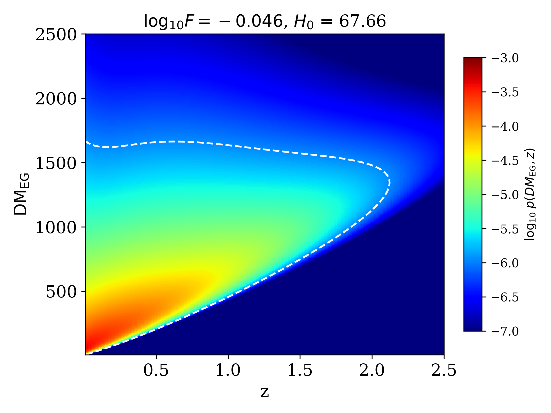
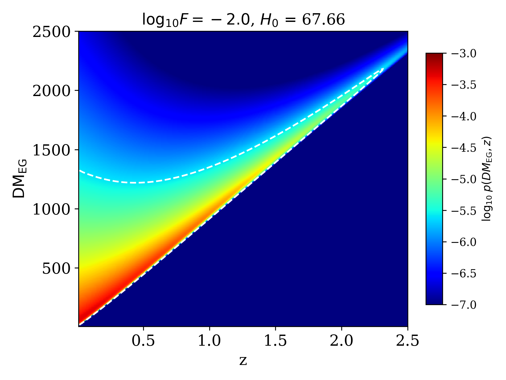
Figure 1: Upper panel: The $p({\rm DM_{\rm EG}}|z)$  distribution which admits a high fluctuation parameter (low galactic feedback efficiency). Lower panel: The $p({\rm DM_{\rm EG}}|z)$  distribution which admits a low fluctuation parameter (high galactic feedback efficiency). The white dashed-line indicates the 95 percentile contour. Note that the distribution primarily falls below the mean due to the rare population of high DM FRBs that result from intersections with the host galaxy and/or very massive galaxy halos along the LOS.

The variance in ${\rm DM}_{\rm EG}$, however, is influenced by both ${\sigma}_{\rm host}$ and $F$. However, at high redshift, the contribution to the variance of ${\rm DM}_{\rm EG}$ due to ${\sigma}_{\rm host}$ may decrease relative to the contributions by ${\rm DM}_{\rm cosmic}$ and, inherently, $F$. In James et al. (2022b), their work assumes that uncertainties attributed to the fixed value of $F$ can be aggregated into uncertainties in ${\sigma}_{\rm host}$; however, at high redshift, the assumption breaks down as the uncertainty in $F$ becomes larger than the true constraint in ${\sigma}_{\rm host}$.

Although Macquart et al. (2020) restrict their fitting of the fluctuation parameter to $F\in[0.09,0.32]$ based on semi-analytic models, we sample a wide range of $F\in[0,1]$. We opt for a logarithmic sampling of the fluctuation parameter to efficiently sample this domain: $\log_{10}F\in[-2,0]$.

The additional parameters used in the model include $H_{0}$ (acceleration of the Universe’s expansion), the ${\rm DM}_{\rm EG}$  contribution due to the FRB host galaxy, and other parameters that govern the FRB luminosity function and redshift distribution. The model assumes that the ${\rm DM}_{\rm EG}$  contribution from the FRB host galaxy can be modeled as a log-normal distribution with a mean of $\mu_{\rm host}$ (or ${\rm DM}_{\rm host}$) and a spread of $\sigma_{\rm host}$.

In terms of the luminosity function, the maximum burst energy is given as $E_{\rm max}$, and the integral slope of the FRB luminosity function is controlled by $\gamma$. The volumetric burst rate ($\Phi$) is controlled by the parameter $n_{\rm sfr}$ assuming a star-formation rate: $\Phi\propto{\rm SFR(z)}^{n_{\rm sfr}}$. Additionally, $\alpha$ is the spectral index that sets a frequency-dependent FRB rate as $\Phi(z,\nu)=\Phi(z)\nu^{\alpha}$ (James et al., 2022b).

2.2 Measuring $F$ Using FRB Survey Data

To measure the fluctuation parameter, we perform a simultaneous fit of the parameters in the zdm model implemented by James et al. (2022b). We obtain the probability distributions of each parameter by a brute-force grid search based on the ranges specified in Table 2, and calculating the likelihoods for each permutation of parameter values.

We fit these parameters using both the FRB sample used in James et al. (2022b) and newly detected or analyzed FRBs (see Table 1) which were collected from the Parkes and ASKAP telescopes. Of this sample of 78 measured FRBs, 57 FRBs do not have measured redshifts. Constraining the redshift of an FRB greatly increases the statistical power as a single FRB with a redshift can have the same constraining power as roughly 20 FRBs without redshifts (James et al., 2022b). Thus our inclusion of seven new CRAFT/ICS FRBs detected over three frequency ranges (four with host redshifts), and our identification of the host galaxy of FRB20211203C at $z=0.344$, provides a significant increase in statistical precision.

There is a slight bias in this sample, as we include FRB20220610A, which has an energy exceeding the previously estimated turnover $E_{\rm max}$ by a factor of 3.5–10, depending on the assumed spectral behavior (Ryder et al., 2022). FRB20210912A has a lower DM of 1234.5 ${\rm pc\,cm^{-3}}$, but it does not have an identified redshift, perhaps due to the distance to its host galaxy (Marnoch et al., in prep). Therefore, the inclusion of some data is redshift-dependent. Given that our sample is statistically limited, we assume the resulting bias to be small compared to the gain in precision.

In contrast to the James et al. (2022b) analysis, we hold model parameters that are not degenerate with $F$ to their fiducial values. These parameters were determined to be non-degenerate with $F$ running the model using a low-resolution grid search on synthetic data to determine if $F$ correlated with any of the other model parameters. From this preliminary analysis, we fix the following parameters that were found to be non-degenerate with $F$: $\alpha$, $\gamma$, $E_{\rm max}$, and $n_{\rm sfr}$. On the other hand, we expect the fluctuation parameter to be degenerate with the other model parameters. In particular, we expect the Hubble constant $H_{0}$–—the cosmological parameter that quantifies the expansion of the universe–—to be degenerate with the fluctuation parameter $F$.

We examine this degeneracy further in Figure 2 which shows the 95 percentile contours for $p({\rm DM}|z)$ for two models with very different $F$ and $H_{0}$ values. One notes that the lower contours (${\rm DM}_{\rm EG}\lesssim 720,\,z\lesssim 1.3$) of both realizations look nearly identical. Although the contours differ above the mean, the bulk of the constraining power on $F$ is in the lower contour or “DM cliff”. Therefore, we anticipate $F$ and $H_{0}$ to be highly correlated.

The distribution at the low DM end of $p({\rm DM_{\rm EG}}|z)$  exhibits a sharp cut-off and provides strong constraints on $H_{0}$ since there is a minimum imparted ${\rm DM}_{\rm cosmic}$  from voids and is not impeded by the ${\rm DM}_{\rm EG}$  contributions from large-scale structures like filaments or halos. And while the contours do have modest differences at high $z$, high ${\rm DM}_{\rm EG}$, these can be difficult to distinguish from host galaxy contributions to ${\rm DM}_{\rm EG}$.

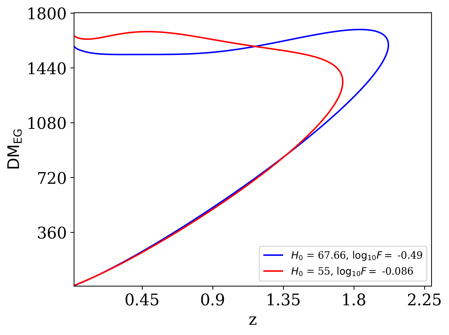
Figure 2: $95^{\rm th}$ percentile contours of two $p({\rm DM_{\rm EG}}|z)$  distributions with different prescriptions on the Hubble constant $H_{0}$ and the fluctuation parameter $F$. Note that the lower contours (“the DM cliff”) of both models are nearly identical to each other. Since the DM cliff places a stronger constraint on $H_{0}$ and $F$ than the upper contour, we expect a high degree of degeneracy between $H_{0}$ and $F$. The units of ${\rm DM}_{\rm EG}$  are in pc cm^-3 and the units of $H_{0}$ are $\rm km\,s^{-1}\,Mpc^{-1}$.

Table 1: New FRB detections detected in 2022 used in addition to the FRB surveys used in James et al. (2022b). The FRB name, SNR-maximizing DM, ${\rm DM}_{\rm ISM}$ estimated using the NE2001 model of Cordes & Lazio (2002b), central frequency of observation $\nu$, measured signal-to-noise ratio SNR, redshift $z$, and original reference. Where redshifts are not given, this is because (a): no voltage data were dumped, preventing radio localization; (b) optical follow-up observations are not yet complete; (c) Substantial Galactic extinction has challenged follow-up optical observations; (d) the host galaxy appears too distant to accurately measure a redshift.

Name	DM	${\rm DM}_{\rm ISM}$	$\nu$	SNR	$z$	Ref.
	(${\rm pc\,cm^{-3}}$)	(${\rm pc\,cm^{-3}}$)	(MHz)
CRAFT/ICS $900\,{\rm MHz}$
20211203C	636.2	63.4	920.5	14.2	0.344	Shannon et al. (in prep.)
20220501C	449.5	30.6	863.5	16.1	0.381
20220725A	290.4	30.7	920.5	12.7	0.1926
CRAFT/ICS $1.3\,{\rm GHz}$
20220531A	727.0	70.0	1271.5	9.7	–	Shannon et al. (in prep.)
20220610A	1458.1	31.0		29.8	1.016	Ryder et al. (2022)
20220918A	656.8	40.7		26.4	–	Shannon et al. (in prep.)
CRAFT/ICS $1.6\,{\rm GHz}$
20220105A	583.0	22.0	1632.5	9.8	0.2785	Shannon et al. (in prep.)
20221106A	344.0	34.8	1631.5	35.1	–

2.3 Forecasting the fluctuation parameter $F$ using Synthetic FRBs

Table 2: z-DM grid parameters

Parameter	Unit	Fiducial	Min	Max	N
$H_{0}$	km s-1 Mpc-1	67.4	60.0	80.0	21
$\log F$	-	0.32	-1.7	0	30
${\mu}_{\rm host}$	$\log{\rm pc\,cm^{-3}}$	2.16	1.7	2.5	10
${\sigma}_{\rm host}$	$\log{\rm pc\,cm^{-3}}$	0.51	0.2	0.9	10
$\log_{10}E_{\rm max}$	$\log{\rm erg}$	41.84	–	–	–
$n_{\rm sfr}$	-	1.77	–	–	–
$\alpha$	-	1.54	–	–	–
$\gamma$	-	-1.16	–	–	–

Note. — This table indicates the parameters of the high-resolution grid run. Non-degenerate parameters are held to the fiducial values. $N$ is the number of cells between the minimum and maximum parameter values.

Future radio surveys are expected to widely increase the number of sub-arcsecond localized FRBs. Thus, the constraining power on $F$ will greatly increase. To explore this scenario we generate a forecast on the fluctuation parameter by replicating our analysis using a synthetic FRB survey. A sample of 100 localized synthetic FRBs was drawn assuming the distribution of FRBs followed the fiducial $z-{\rm DM}$ distribution (Table 2). With this synthetic survey, we calculate the associated 4D likelihood matrix and make a forecast on the fluctuation parameter by adopting different priors on $H_{0}$.

3 Results

3.1 Parameter Likelihoods from FRB Surveys

In Figure 3, we present the 1D PDFs of each parameter determined from the 78 FRBs collected from the ASKAP and Parkes Radio Telescopes. In comparison to James et al. (2022b), there is a significant loss of constraining power on $H_{0}$ by including $F$ as a free parameter. We measure a Hubble constant to be $85.3_{-8.1}^{+9.4}$  which is 1.5 times more uncertain than the $H_{0}$ measurement in James et al. (2022b). We attribute the uncertainty to the degeneracy between $H_{0}$ and $F$ as indicated by the strong anti-correlation in Figures 2 and 5.

To understand how our survey data at different frequencies contribute to the constraining power on $H_{0}$ and $F$, we replicate the survey contribution determination from James et al. (2022b) which provides the 1D parameter likelihood across different FRB surveys with the Murriyang (Parkes) and Australian Square Kilometre Array (ASKAP). Figure 4 shows the 1D PDFs of $H_{0}$ and $\log_{10}F$ across the different surveys used in this analysis. We observe that the CRAFT 1.3 GHz and 900 MHz surveys tend to have stronger constraining power as they contain more FRBs with measured distances (10 and 7 redshifts respectively) than the rest of the surveys.

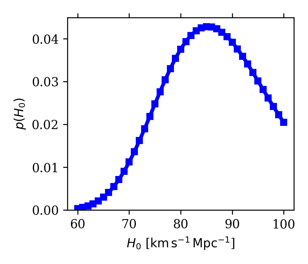
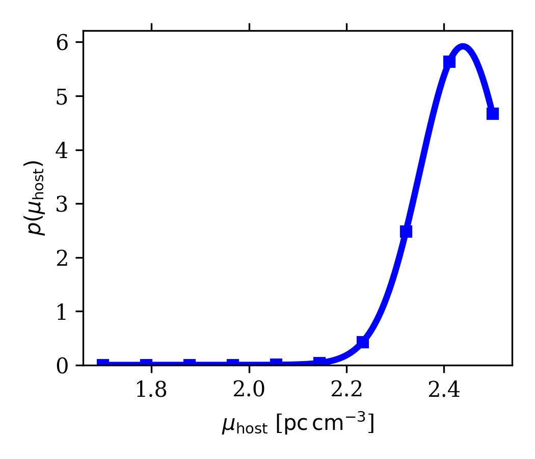
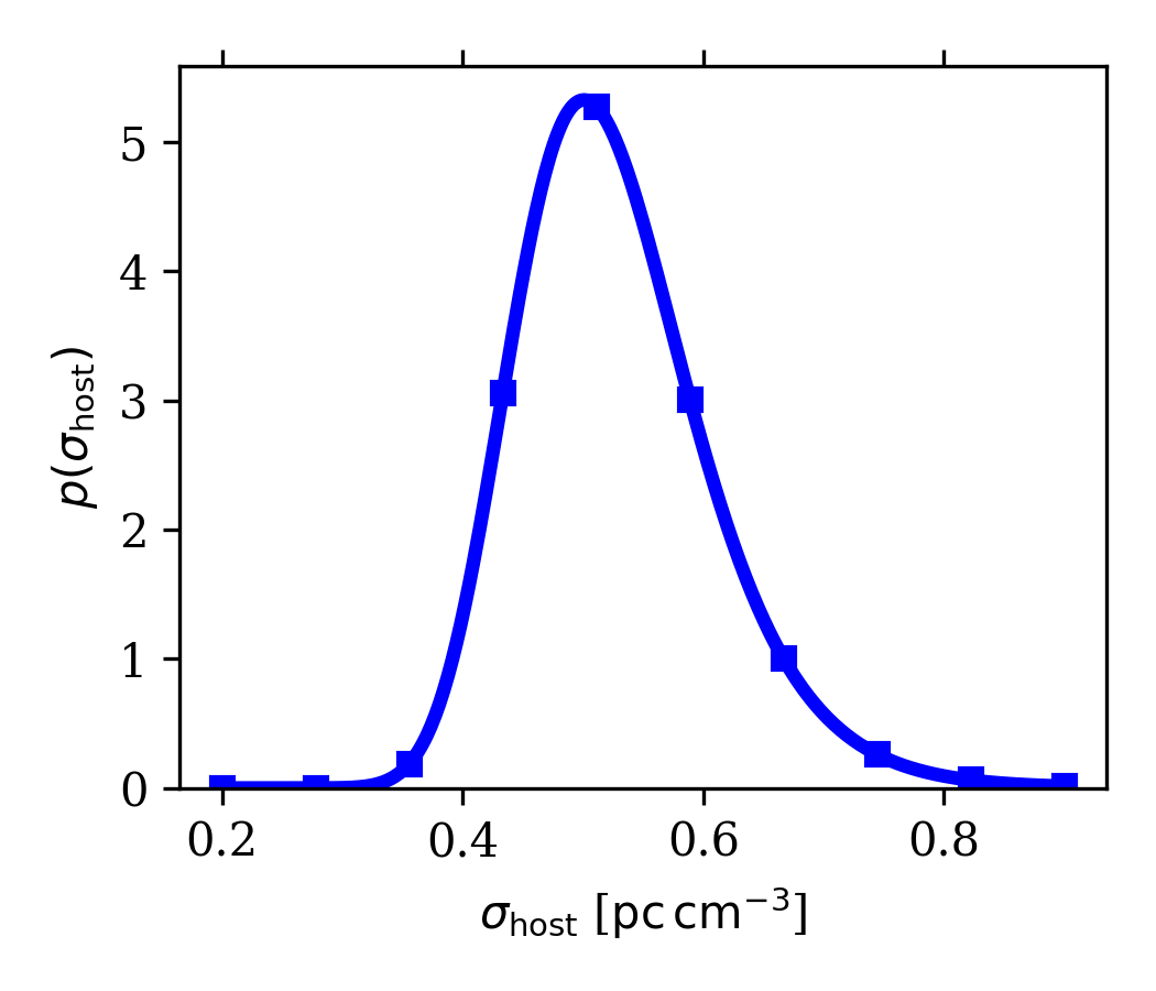
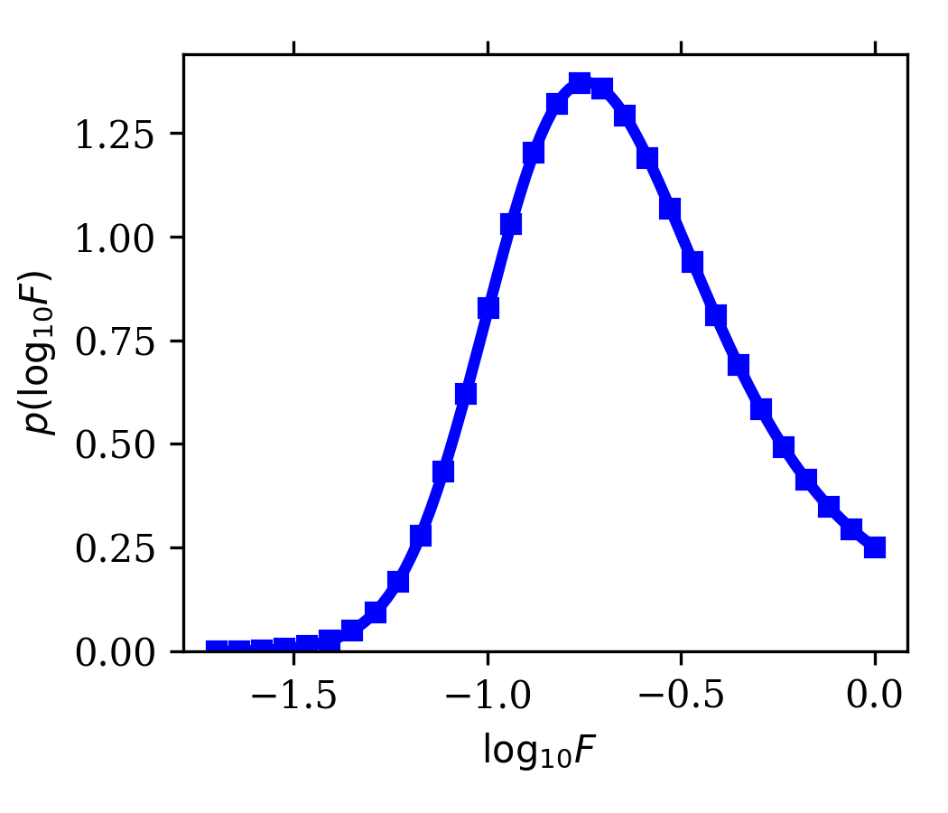
Figure 3: The calculated 1D likelihood functions using 78 FRBs (21 FRBs with redshifts). $F$ is measured to be $\log_{10}F=-0.75_{-0.25}^{+0.33}$ with no priors on $H_{0}$. There is a loss of constraining power on $H_{0}$ compared to the measurement by James et al. (2022b) when allowing the $F$ parameter to vary.

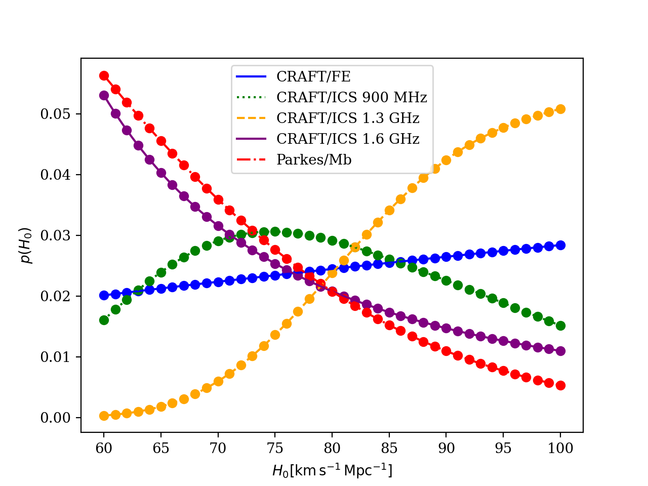
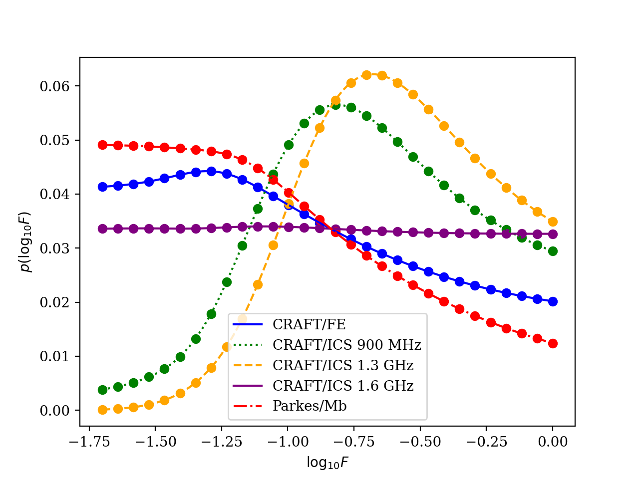
Figure 4: Upper panel: 1D likelihood functions of $H_{0}$ based on different FRB surveys used in this work. Compared to the survey contribution constraints (see Figure 7 in James et al., 2022b), the constraining power of each survey is diminished. Lower panel: Same as upper panel for likelihood functions of $\log_{10}F$. The CRAFT/ICS 900 MHz and 1.3 GHz surveys provide the most constraining power on $F$ and $H_{0}$ as they contain more redshifts than the other surveys.

In Figure 5, we present the 2D likelihoods of each parameter against $F$. We observe correlations between $F$ and the FRB host galaxy parameters (${\mu}_{\rm host}$, ${\sigma}_{\rm host}$), which we expect to be degenerate given that they both influence the variance of $\langle{\rm DM}_{\rm cosmic}\rangle$. As expected from Figure 2, the degeneracy in the lower bound (or cliff) of the $z$-DM_EG  distribution results in the strong anti-correlation of $H_{0}$ and $F$, resulting in a loss of constraining power on $H_{0}$ when allowing $F$ to vary.

Our initial simultaneous fit does not implement any priors on the model parameters. As motivated by the $H_{0}$-$F$ degeneracy in Figure 2, we determine the 1D likelihoods of $\log_{10}F$ by limiting our grid to different values of $H_{0}$. We consider a uniform prior on $H_{0}$ between 67.4 and 73.04 ${\rm km\,s^{-1}\,Mpc^{-1}}$—the lower bound is motivated by the $H_{0}$ constraint from Planck Collaboration et al. (2020), and the upper bound is motivated by cosmological constraints using type-1a supernovae (SNe) from Riess et al. (2022).

In Figure 6, we present the 1D likelihood of the fluctuation parameter assuming different priors on $H_{0}$. Assuming a uniform prior between the CMB and SNe-derived values of $H_{0}$, we measure the fluctuation parameter to be $\log_{10}F=-0.48^{+0.26}_{-0.18}$ within $1\sigma$ ($\log_{10}F=\log_{10}F>-0.89$ with 99.7% confidence). We present all measurements of the $F$ parameter with different priors on $H_{0}$ in Table 3.

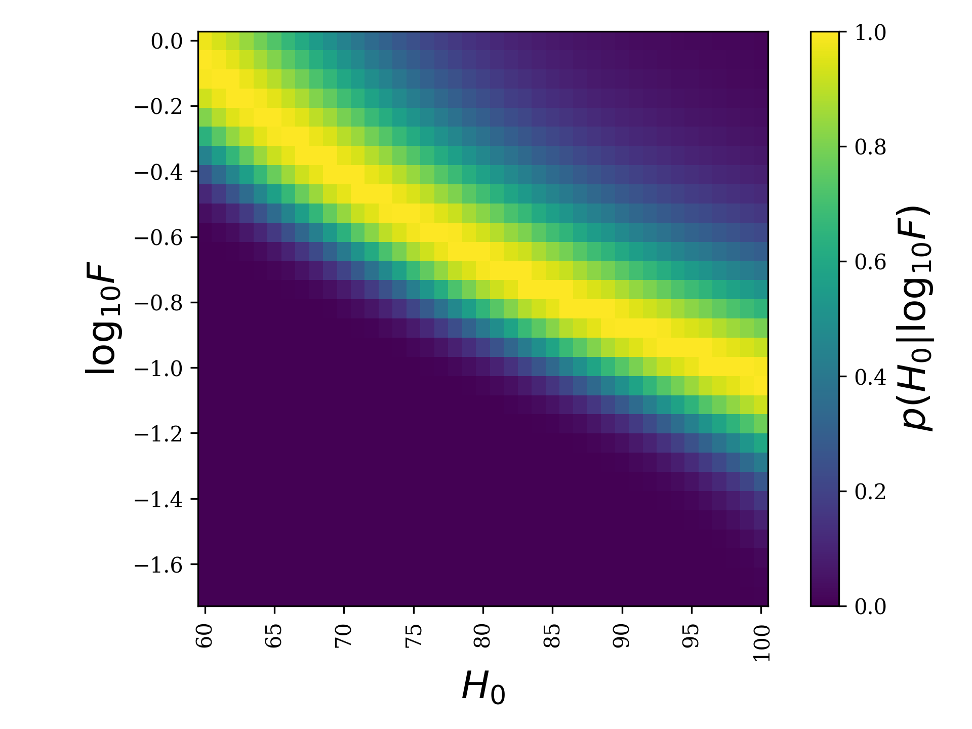
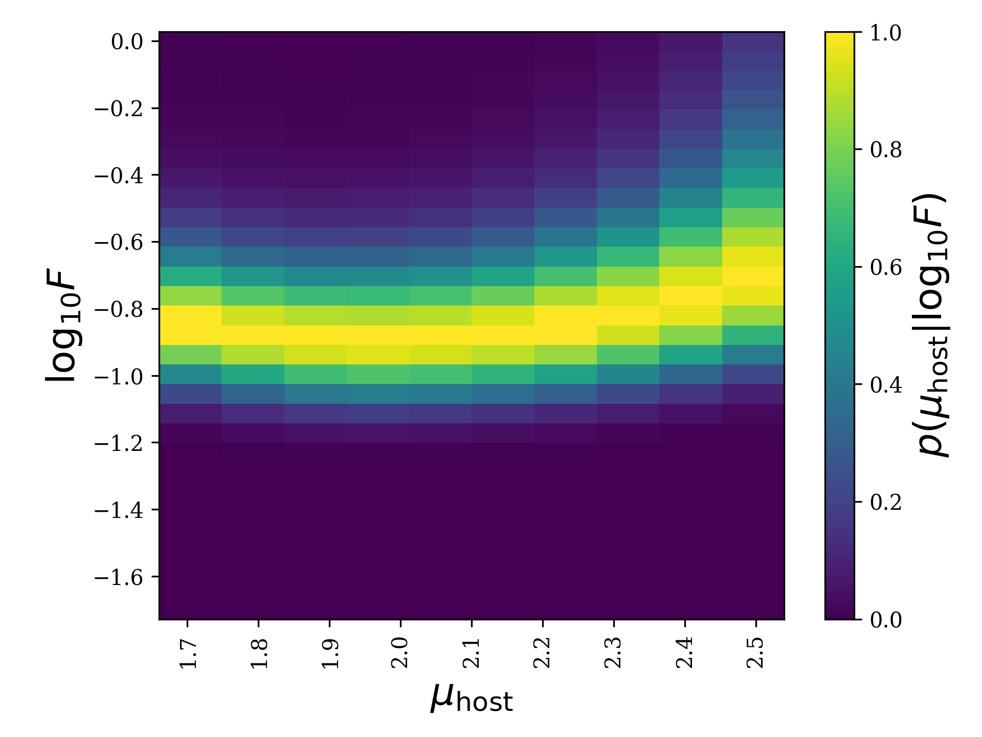
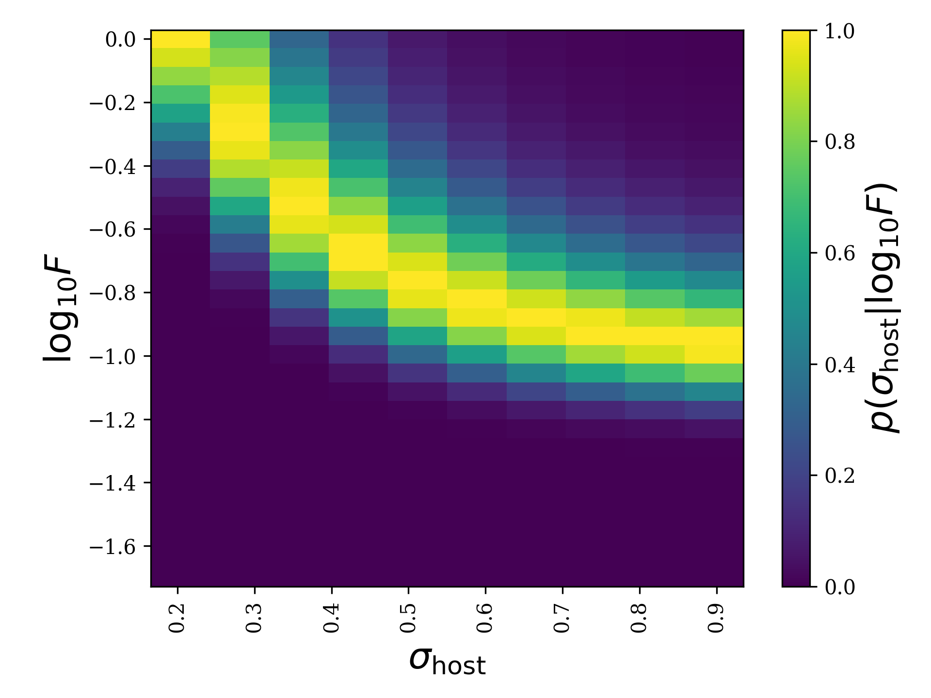
Figure 5: The 2D likelihood functions for each parameter compared against $\log_{10}F$ derived from 78 FRBs (21 FRBs with redshifts). There is a strong anti-correlation between $F$ and $H_{0}$. Additionally, we observe strong correlations between $F$ and the host galaxy ${\rm DM}_{\rm EG}$  contribution (${\mu}_{\rm host},{\sigma}_{\rm host}$).

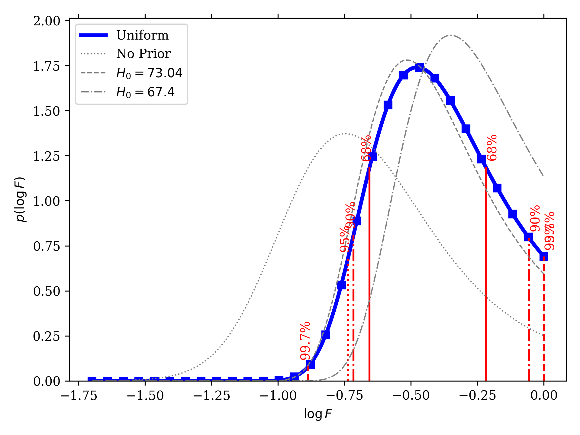
Figure 6: 1D survey likelihoods of $\log_{10}F$ assuming different priors on $H_{0}$. The dotted gray line is the original 1D likelihood without any priors on $H_{0}$. The blue line is the likelihood which adopts a uniform prior on $H_{0}\in[67.4,73.04]$. The dashed gray line is the likelihood adopting $H_{0}=67.0\,{\rm kms^{-1}Mpc^{-1}}$. The dash-dotted gray line is the likelihood adopting $H_{0}=73.0\,{\rm kms^{-1}Mpc^{-1}}$. Adopting a prior on $H_{0}$ or fixing the values of $H_{0}$ greatly improves the constraint on $F$.

Table 3: Measurements of the $F$ Parameter

Survey	No Prior	Uniform $H_{0}$ Prior	CMB $H_{0}$	SNe $H_{0}$
Observed	$-0.75_{-0.25}^{+0.33}$	$-0.48^{+0.26}_{-0.18}$	$-0.35_{-0.15}^{+0.23}$	$-0.52_{-0.17}^{+0.26}$
Synthetic	$-0.58_{-0.15}^{+0.15}$	$-0.60_{-0.10}^{+0.09}$	$-0.52_{-0.06}^{+0.07}$	$-0.67_{-0.06}^{+0.06}$

Note. — This table lists the measurements of the $F$ parameter from the observational FRB survey (76 localized FRBs with 16 redshifts) and the synthetic CRACO survey (100 localized FRBs; all with redshifts). The measurements are presented without a prior, a uniform prior between the CMB ($H_{0}=67.0\,{\rm km\,s^{-1}\,Mpc^{-1}}$) and SNe ($H_{0}=73.0\,{\rm km\,s^{-1}\,Mpc^{-1}}$) with their respective Gaussian errors on each side, and fixing $H_{0}$ to the CMB or SNe estimates.

3.2 Parameter Likelihoods from Synthetic Surveys

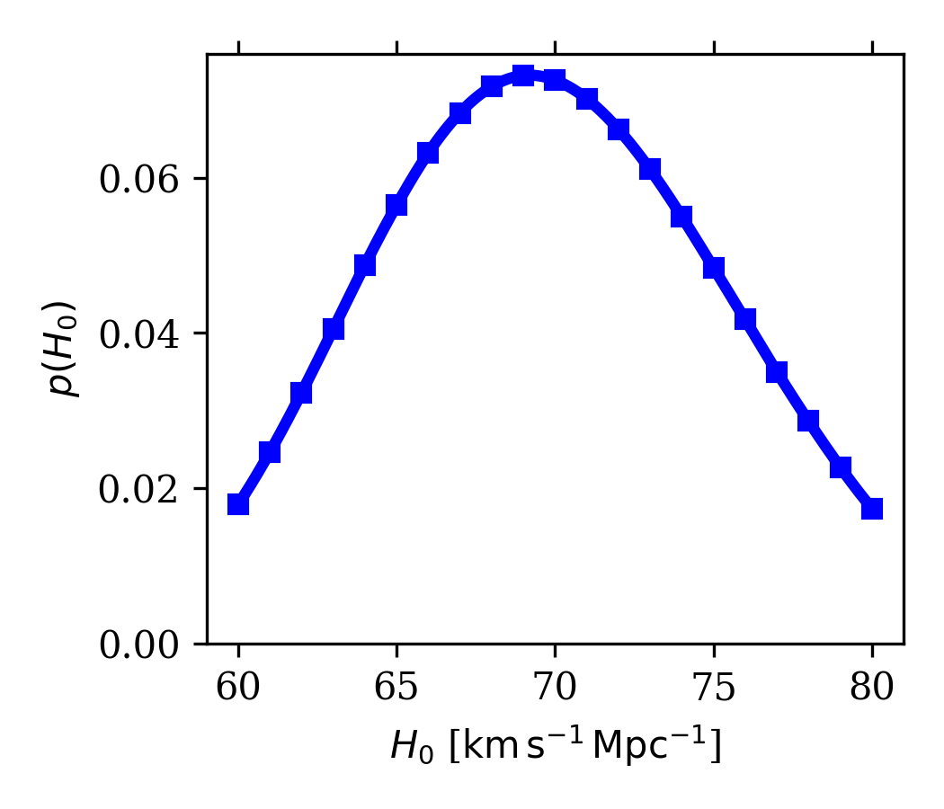
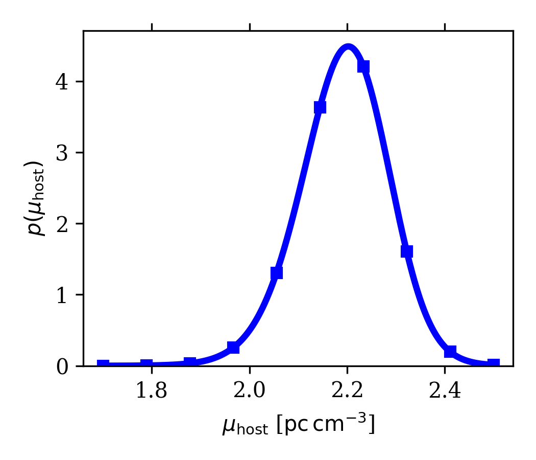
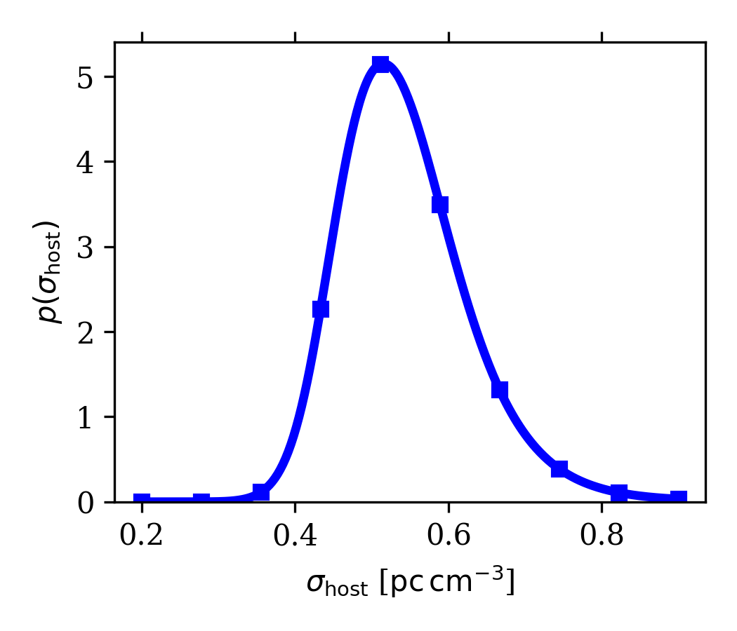
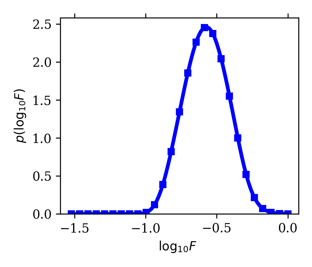
Figure 7: The 1D likelihood functions for each parameter using 100 synthetic FRBs. The constraint on $F$ is enhanced as the uncertainty due to sample size is reduced. Similarly, the constraint on $H_{0}$ is improved compared to the observational fit with only 21 redshifts.

We use a synthetic sample of 100 localized CRACO FRBs to investigate the improvement in constraining power on both $F$ and $H_{0}$. In Figure 7, we present the PDFs of each parameter in the grid. We observe that the constraint on $H_{0}$ has significantly improved by a factor of 1.7 and is more Gaussian than the previous run with $69.2_{-4.9}^{+5.5}$. Assuming a survey of 100 localized FRBs, the best measurement we can make on $H_{0}$ if we adopt a Gaussian prior on $\log_{10}F$ (assuming $1\sigma$ corresponds to a 20% error in the measurement) is $67.6_{-3.4}^{+3.5}\,{\rm km\,s^{-1}\,Mpc^{-1}}$ (see Table 4).

In Figure 8 we show posterior estimates for $\log_{10}F$ using different priors (see Table 3). Using the uniform prior, we obtain a forecast on the fluctuation parameter of $\log_{10}F=-0.60_{-0.18}^{+0.19}$ within $2\sigma$. We note that when compared to Figure 3, there is a definitive upper limit on the fluctuation parameter rather than only a lower limit. Incorporating the uniform prior enhances the constraint on $F$ by a factor of $\sim 1.5$, and fixing the value of $H_{0}$ can increase the constraint by a factor of $2.5$.

Figure 8: Same as Figure 6 but based on fits to the synthetic FRB sample. Assuming a uniform prior between CMB and SNe values of $H_{0}$ equipped with their associated Gaussian errors on both sides, we find $\log_{10}F=-0.60_{-0.10}^{+0.09}$. Fixing the value of $H_{0}$ also greatly enhances the constraint on $F$ by a factor of $>1.5$.

Table 4: Measurements of $H_{0}$

Survey	No Prior	Gaussian Prior
Observed	$85.3_{-8.1}^{+9.4}$	-
Synthetic	$69.2_{-4.9}^{+5.5}$	$67.6_{-3.4}^{+3.5}$

Note. — This table lists the measurements of $H_{0}$ from the observational FRB survey (76 localized FRBs with 16 redshifts) and the synthetic CRACO survey (100 localized FRBs; all with redshifts). The measurements are presented without a prior on $F$ and a Gaussian prior on $F$ centered at $\log_{10}F\simeq-0.49$ with $\sigma\simeq 0.1$ (20% error on $F$).

4 Discussion

4.1 Measurement of the fluctuation parameter

Our principle result from the population analysis of 78  FRBs (21 with redshifts) is a lower limit on $F$ which is $\log_{10}F=-0.48^{+0.26}_{-0.18}$ ($\log_{10}F>-0.89$  at 99.7% confidence). This measurement is motivated by James et al. (2022b), where they noted that for future localization of FRBs beyond $z\gtrsim 1$, $F$ may need to be fitted explicitly. We note that this observation is only made when adopting a prior between the CMB and SNe values of $H_{0}$.

4.2 Fluctuation Parameter Degeneracies

Our findings indicate a strong degeneracy between the Hubble constant $H_{0}$ and the fluctuation parameter $F$ when simultaneously fitting both within the z-DM modeling framework adopted by James et al. (2022a) which uses $F=0.32$ which falls within the accepted range of our measurement.

Aside from the degeneracy between $F$ and $H_{0}$, we would like to call attention to the possible degeneracy between $F$ and $\sigma_{8}$–the RMS amplitude of the matter density field when smoothed with an $8h^{-1}$ Mpc filter. In the case of w feedback ($F\rightarrow 1$), more mass would be concentrated within cosmic filaments, increasing the variance of a fixed-mass filter (i.e., $\sigma_{8}$). We expect these two parameters to be inversely coupled. A preliminary analysis varying $\sigma_{8}$ in the CAMELS IllustrisTNG cosmological simulations does show a positive correlation between $F$ and $\sigma_{8}$ (Medlock et al. in prep.).

4.3 Forecasting enhanced constraints on $F$

Using a sample of 100 synthetic FRBs (see Figure 8), we are able to constrain both upper and lower limits on the fluctuation parameter out to $3\sigma$. Since we are only able to effectively constrain a lower limit on $F$, we compare the lower-sided half-maximum widths. We find the left-sided half-maximum width of the synthetic distribution is half the width of the current measured distribution. We expect this constraint to only improve with more localizations, which will be easily facilitated with next-generation all-sky radio observatories.

Additionally, it is of interest to see how this method compares to other ways of measuring the baryon distribution in the IGM. For example, an alternative method to constrain AGN and stellar feedback focuses on small-scale deviations in the matter power spectrum (van Daalen et al., 2020). As baryonic feedback significantly influences the mass distribution at smaller scales (higher $k$), probes of the gas density at those scales (thermal Sunyaev-Zel’dovich effect) can measure the intergalactic baryon distribution (Pandey et al., 2023).

4.4 Comparing with Fluctuation Parameter in IllustrisTNG

In a work by Zhang et al. (2021) to highlight the utility of FRBs in probing the IGM, they generated thousands of FRB sightlines in IllustrisTNG and fitted the observed extragalactic DM excess $p_{\rm cosmic}(\Delta)$. They provide the fitted parameters as well as the dispersion in the $z$-DM_EG  distribution $\sigma_{\rm DM}$. We convert these values into the fluctuation parameter $F$ by assuming $\sigma_{\rm DM}=Fz^{-0.5}$.

In Figure 9, we present these derived $\log_{10}F$ values as a function of redshift compared to our measured values. Between $0.4<z<2$, our measurements are in fine agreement. However, we observe that the fluctuation parameter in Illustris appears to be higher at $z\lesssim 0.4$ and lower when $z>2$.

From the redshift-dependent ${\rm DM}_{\rm IGM}$ distributions derived from IllustrisTNG (figure 2 from Zhang et al. (2021)), distributions between $0.1<z<0.4$ are wider and the modes of each distribution are spread further apart. This may explain why the IllustrisTNG fluctuation parameter is higher than our measurement as the ${\rm DM}_{\rm IGM}$ distribution functions have larger variance at those redshifts.

To make a proper comparison between our work and Zhang et al. (2021), it may be necessary to introduce a free parameter for the redshift evolution of $\sigma_{\rm DM}$ instead of simply fixing the redshift exponent to $-1/2$ (Equation 2).

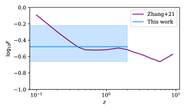
Figure 9: Fluctuation parameters derived from this work, the fiducial value from James et al. (2022b), and the IllustrisTNG values from Zhang et al. (2021). Our measurement on $F$ agrees with the simulated $F$ parameter between $0.4<z<2$.

5 Conclusions

In this work, we have implemented variance in ${\rm DM}_{\rm cosmic}$ as a free parameter in a forward model of the $z$-DM_EG  distribution of FRBs. With this adapted model and a survey of 78 ASKAP and Parkes FRBs, we constrain a value for the fluctuation parameter, explore degeneracies within the model, and generate a forecast of the constraint on the fluctuation parameter with a synthetic survey of 100 localized FRBs. The conclusions we draw from this analysis are:

• Incorporating survey data of 78 (21 with redshifts) FRBs yields a firm lower limit on $F$. We place the lower limit on $F$ as measured by the survey sample to be $\log_{10}F>-0.89$ at 99.7% confidence. The 900 MHz and 1.3 GHz surveys dominate this constraint due to their higher number of localizations to host galaxies and their associated redshifts.

• Forward modeling the FRB data from Parkes and ASKAP, the fluctuation parameter is degenerate with the Hubble constant $H_{0}$.

• We forecast that 100 localized FRBs are sufficient to constrain both an upper and lower limit on the fluctuation parameter. With the greater count of localizations, the half-maximum width of the distribution decreases by $\approx 50\%$.

• Extrapolation of the fluctuation parameter from IllustrisTNG shows agreement between $0.4<z<2.0$. Zhang et al. (2021) measure a higher fluctuation parameter at low redshift ($z<0.4$) and a lower fluctuation parameter beyond $z>2$. The former result is likely to be an effect of the rapidly evolving ${\rm DM}_{\rm IGM}$ distribution at low redshift.

Next-generation radio observatories will significantly improve the constraint on the fluctuation parameter. For example, the Deep Synoptic Array 2000 (DSA-2000) is expected to localize on the order of 10,000 FRBs each year — enough FRBs to sufficiently characterize the baryonic contents of the IGM (Hallinan et al., 2019; Ravi et al., 2019).

Additionally, the FRB Line-of-sight Ionization Measurement From Lightcone AAOmega Mapping (FLIMFLAM) survey is an upcoming spectroscopic survey that seeks to map the intervening cosmic structures and diffuse cosmic baryons in front of localized FRBs (Lee et al., 2022). These FRB foreground data taken in the Southern hemisphere will be used in conjunction with ASKAP FRB measurements to improve the constraints on the intergalactic baryon distribution (Lee et al., 2022).

These expansions in FRB surveys with localizations are expected to greatly improve the constraints on the fluctuation parameter. With these improved constraints on $F$, one may leverage this novel observable for investigating feedback and cosmological prescriptions in simulations.

Combining the $F$ parameter with other observables like the thermal SZ effect that trace the intergalactic baryon distribution, there is ample opportunity to better inform subgrid feedback models (Muñoz & Loeb, 2018; Pandey et al., 2023).

References

- Aggarwal et al. (2021) Aggarwal, K., Budavári, T., Deller, A. T., et al. 2021, ApJ, 911, 95, doi: 10.3847/1538-4357/abe8d2
- Appleby et al. (2021) Appleby, S., Davé, R., Sorini, D., Storey-Fisher, K., & Smith, B. 2021, MNRAS, 507, 2383, doi: 10.1093/mnras/stab2310
- Ayromlou et al. (2023) Ayromlou, M., Kauffmann, G., Anand, A., & White, S. D. M. 2023, MNRAS, 519, 1913, doi: 10.1093/mnras/stac3637
- Cen & Ostriker (2006) Cen, R., & Ostriker, J. P. 2006, ApJ, 650, 560, doi: 10.1086/506505
- Cook et al. (2023) Cook, A. M., Bhardwaj, M., Gaensler, B. M., et al. 2023, ApJ, 946, 58, doi: 10.3847/1538-4357/acbbd0
- Cordes & Lazio (2002a) Cordes, J. M., & Lazio, T. J. W. 2002a, arXiv e-prints, astro. https://arxiv.org/abs/astro-ph/0207156
- Cordes & Lazio (2002b) —. 2002b, ArXiv Astrophysics e-prints
- Davé et al. (2019) Davé, R., Anglés-Alcázar, D., Narayanan, D., et al. 2019, MNRAS, 486, 2827, doi: 10.1093/mnras/stz937
- Davé et al. (2011) Davé, R., Oppenheimer, B. D., & Finlator, K. 2011, MNRAS, 415, 11, doi: 10.1111/j.1365-2966.2011.18680.x
- Fukugita et al. (1998) Fukugita, M., Hogan, C. J., & Peebles, P. J. E. 1998, ApJ, 503, 518, doi: 10.1086/306025
- Hallinan et al. (2019) Hallinan, G., Ravi, V., Weinreb, S., et al. 2019, in Bulletin of the American Astronomical Society, Vol. 51, 255, doi: 10.48550/arXiv.1907.07648
- James et al. (2022a) James, C. W., Prochaska, J. X., Macquart, J. P., et al. 2022a, MNRAS, 509, 4775, doi: 10.1093/mnras/stab3051
- James et al. (2022b) James, C. W., Ghosh, E. M., Prochaska, J. X., et al. 2022b, MNRAS, 516, 4862, doi: 10.1093/mnras/stac2524
- Kereš et al. (2005) Kereš, D., Katz, N., Weinberg, D. H., & Davé, R. 2005, MNRAS, 363, 2, doi: 10.1111/j.1365-2966.2005.09451.x
- Lee et al. (2022) Lee, K.-G., Ata, M., Khrykin, I. S., et al. 2022, ApJ, 928, 9, doi: 10.3847/1538-4357/ac4f62
- Lorimer et al. (2007) Lorimer, D. R., Bailes, M., McLaughlin, M. A., Narkevic, D. J., & Crawford, F. 2007, Science, 318, 777, doi: 10.1126/science.1147532
- Macquart et al. (2020) Macquart, J. P., Prochaska, J. X., McQuinn, M., et al. 2020, Nature, 581, 391, doi: 10.1038/s41586-020-2300-2
- McQuinn (2014) McQuinn, M. 2014, ApJ, 780, L33, doi: 10.1088/2041-8205/780/2/L33
- Muñoz & Loeb (2018) Muñoz, J. B., & Loeb, A. 2018, Phys. Rev. D, 98, 103518, doi: 10.1103/PhysRevD.98.103518
- Pandey et al. (2023) Pandey, S., Lehman, K., Baxter, E. J., et al. 2023, arXiv e-prints, arXiv:2301.02186, doi: 10.48550/arXiv.2301.02186
- Planck Collaboration et al. (2020) Planck Collaboration, Aghanim, N., Akrami, Y., et al. 2020, A&A, 641, A6, doi: 10.1051/0004-6361/201833910
- Prochaska & Zheng (2019) Prochaska, J. X., & Zheng, Y. 2019, MNRAS, 485, 648, doi: 10.1093/mnras/stz261
- Ravi et al. (2019) Ravi, V., Battaglia, N., Burke-Spolaor, S., et al. 2019, BAAS, 51, 420, doi: 10.48550/arXiv.1903.06535
- Ravi et al. (2023) Ravi, V., Catha, M., Chen, G., et al. 2023, arXiv e-prints, arXiv:2301.01000, doi: 10.48550/arXiv.2301.01000
- Riess et al. (2022) Riess, A. G., Yuan, W., Macri, L. M., et al. 2022, ApJ, 934, L7, doi: 10.3847/2041-8213/ac5c5b
- Ryder et al. (2022) Ryder, S. D., Bannister, K. W., Bhandari, S., et al. 2022, arXiv e-prints, arXiv:2210.04680, doi: 10.48550/arXiv.2210.04680
- Shull et al. (2012) Shull, J. M., Smith, B. D., & Danforth, C. W. 2012, ApJ, 759, 23, doi: 10.1088/0004-637X/759/1/23
- Sorini et al. (2022) Sorini, D., Davé, R., Cui, W., & Appleby, S. 2022, MNRAS, 516, 883, doi: 10.1093/mnras/stac2214
- van Daalen et al. (2020) van Daalen, M. P., McCarthy, I. G., & Schaye, J. 2020, MNRAS, 491, 2424, doi: 10.1093/mnras/stz3199
- Zhang et al. (2021) Zhang, Z. J., Yan, K., Li, C. M., Zhang, G. Q., & Wang, F. Y. 2021, ApJ, 906, 49, doi: 10.3847/1538-4357/abceb9