Subword Segmental Machine Translation:
Unifying Segmentation and Target Sentence Generation

Abstract

Subword segmenters like BPE operate as a preprocessing step in neural machine translation and other (conditional) language models. They are applied to datasets before training, so translation or text generation quality relies on the quality of segmentations. We propose a departure from this paradigm, called subword segmental machine translation (SSMT). SSMT unifies subword segmentation and MT in a single trainable model. It learns to segment target sentence words while jointly learning to generate target sentences. To use SSMT during inference we propose dynamic decoding, a text generation algorithm that adapts segmentations as it generates translations. Experiments across 6 translation directions show that SSMT improves chrF scores for morphologically rich agglutinative languages. Gains are strongest in the very low-resource scenario. SSMT also learns subwords that are closer to morphemes compared to baselines and proves more robust on a test set constructed for evaluating morphological compositional generalisation.

1 Introduction

The continued success of neural machine translation (NMT) can be partially attributed to effective subword segmenters. Algorithms like byte-pair encoding (BPE) (Sennrich et al., 2016) and Unigram LM (ULM) (Kudo, 2018) are computationally efficient preprocessing steps that enable smaller vocabularies and open-vocabulary models.

These methods have proved quite effective, but fall short in certain contexts. For morphologically complex languages they are sub-optimal (Klein and Tsarfaty, 2020) and inconsistent (Meyer and Buys, 2022). This is amplified in low-resource settings (Zhu et al., 2019; Wang et al., 2021; Ács, 2019), where handling rare words is crucial. These issues can be partially attributed to the fact that subword segmentation is separated from model training. BPE and ULM are applied to the training corpus before training starts, so models are reliant on their output. This is not ideal, since these algorithms do not learn segmentations that optimise model performance.

He et al. (2020) address this issue by proposing dynamic programming encoding (DPE), which trains an NMT model that marginalises over target sentence segmentations. After training they apply their model as a subword segmenter by computing the maximising segmentations. DPE is still a preprocessing step (a separate vanilla NMT model is trained on a corpus segmented by DPE), but since its segmentations are trained on MT, they are at least connected to the task at hand.

Train
I do understand.	$\rightarrow$	Ndi-ya-qonda.
I am tired.	$\rightarrow$	Ndi-diniwe.
Where are you from?	$\rightarrow$	U-vela phi?
Are you busy?	$\rightarrow$	Ingaba u-xakekile?
Test
Do you understand?	$\rightarrow$	U-ya-qonda?
I am busy.	$\rightarrow$	Ndi-xakekile.

Table 1: Parallel English-Xhosa sentences with morphologically segmented Xhosa words. The train/test split shows why its critical to accurately model morphemes and morphological compositional generalisation i.e. novel combinations of known morphemes.

In this paper we go one step further by fully unifying NMT and subword segmentation. We propose subword segmental machine translation (SSMT), an end-to-end NMT model that learns subword segmentation during training and can be used directly for inference. It is trained with a dynamic programming algorithm that enables learning subword segmentations that optimise its MT training objective. The architecture is a Transformer-based adaptation of the subword segmental language model (SSLM) (Meyer and Buys, 2022) for the joint task of MT and target-side segmentation.

We also propose dynamic decoding, a decoding algorithm for subword segmental models that dynamically adapts subword segmentations as it generates translations. The fact that our model can be used directly to generate translations sets it apart from existing segmenters. SSMT is not a preprocessing step in any sense — it is single model that learns how to translate and how to segment words, and it can be used to generate translations.

We evaluate on English $\rightarrow$ (Xhosa, Zulu, Swati, Finnish, Tswana, Afrikaans). As shown in table 2, these languages span 3 morphological typologies and several levels of data availability, so they provide a varied test suite to evaluate subword methods across different linguistic contexts. SSMT outperforms baselines on languages that are agglutinating and conjunctively written (the highest morphological complexity), but is outperformed on simpler morphologies. SSMT achieves its biggest gains on Swati, which is our most data scarce language. We conclude that SSMT is justified for morphologically complex languages and especially useful when the languages are low-resourced.

We analyse the linguistic plausibility of SSMT by applying it to unsupervised morphological segmentation. SSMT subwords are closer to morphemes than our baselines. Lastly, we adapt the methods of Keysers et al. (2020) to construct an MT test set for morphological compositional generalisation — the ability to generalise to previously unseen combinations of morphemes. The performance of all models degrade on the more challenging test set, but SSMT exhibits the greatest robustness. We posit that SSMT’s performance gains on morphologically complex languages are due to its morphologically consistent segmentations and its superior modelling of morphological composition.

2 Related Work

Subword segmentation has been widely adopted in NLP. Several algorithms have been proposed, with BPE (Sennrich et al., 2016) and ULM (Kudo, 2018) among the most popular. BPE starts with an initial vocabulary of characters and iteratively adds frequently co-occuring subwords. ULM starts with a large initial vocabulary and iteratively discards subwords based on the unigram language model likelihood. Both of these exemplify the dominant paradigm in NLP: subword segmentation as a preprocessing step. Segmenters are applied to datasets before models are trained on the segmented text.

Language	Morphology	Orthography	Sentences
Xhosa	agglutinative	conjunctive	8.7mil
Zulu			3.9mil
Finnish			1.6mil
Swati			165k
Tswana	agglutinative	disjunctive	5.9mil
Afrikaans	analytic	disjunctive	1.6mil

Table 2: Morphological typology and training data sizes for the target languages used in our experiments.

There are downsides to relegating subword segmentation to the domain of preprocessing. The algorithms are task-agnostic. BPE is essentially a compression algorithm (Gage, 1994), while ULM assumes independence between subword occurrences. Neither of these strategies are in any way connected to the task for which the subwords will eventually be used (in our case machine translation). Ideally subword segmentation should be part of the learnable parameters of a model, so that it can be adjusted to optimise the training objective.

There has been some research on unifying subword segmentation and machine translation. Following recent character-based language models (Clark et al., 2022; Tay et al., 2022), there has been work on character-level NMT models that learn latent subword representations (Edman et al., 2022). However, Libovický et al. (2022) found that subword NMT models still outperform their character-level counterparts. Kreutzer and Sokolov (2018) learn source sentence segmentation during training and find that models prefer character-level segmentations. DPE (He et al., 2020) learns target sentence segmentation during training and is then applied as a subword segmenter.

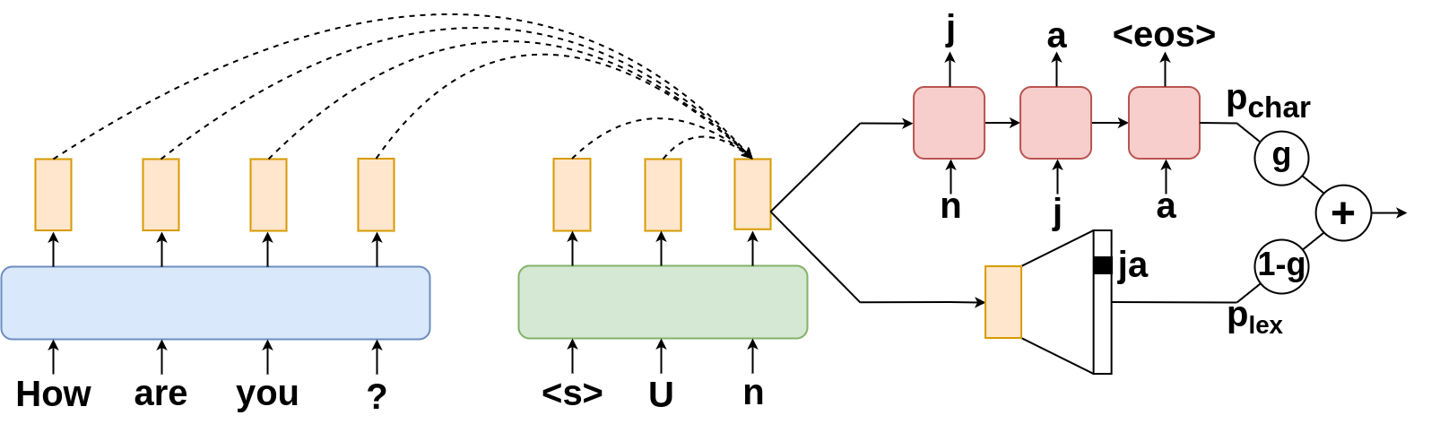
Figure 1: SSMT translates “How are you?” to the Zulu “Unjani?”, computing the probability for subword “ja”. A Transformer encoder-decoder encodes the BPE-segmented source sentence and character-level target sentence. A mixture between a character decoder and lexicon model (Equation 3.1) produces the next subword probability.

This line of work is related to a more general approach known as segmental sequence modelling, where sequence segmentation is viewed as a latent variable to be marginalised over during training. It was initially proposed for tasks like handwriting recognition (Kong et al., 2016) and speech recognition (Wang et al., 2017). Subsequently segmental language models (SLMs) have been proposed for unsupervised Chinese word segmentation (Sun and Deng, 2018; Kawakami et al., 2019; Downey et al., 2021). This was adapted for subword segmentation by Meyer and Buys (2022), who proposed subword segmental language modelling (SSLM). This is the line of work we build on in this paper, adapting subword segmental modelling for NMT.

Our model contrasts with DPE in a few ways. Firstly, our lexicon consists of the $V$ most frequent character n-grams, so unlike DPE we don’t rely on BPE to build the vocabulary. Secondly, we supplement our subword model with a character decoder, which is capable of generating out-of-vocabulary subwords. Lastly, through our proposed dynamic decoding we use SSMT directly to generate translations, instead of having to train an additional NMT model from scratch on our segmentations.

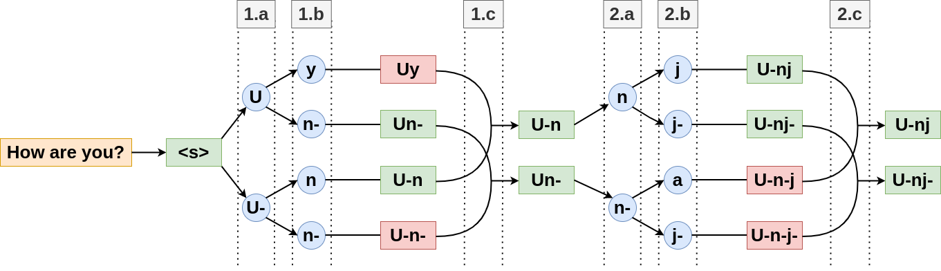
Figure 2: Dynamic decoding for the first 2 characters of a translation (“-” are subword boundaries). Step (a) produces candidate characters that continue and end the subword. Step (b) peaks one character ahead. Step (c) finalises the segmentation decision. Green sequences are chosen ahead of red ones based on higher sequence probabilities.

3 Subword Segmental Machine Translation (SSMT)

3.1 Architecture

SSMT is a Transformer-based encoder-decoder (Figure 1). The encoder is that of a vanilla Transformer NMT model. Source language sentences are pre-segmented with BPE. The decoder adapts the subword segmental architecture of Meyer and Buys (2022) to be Transformer-based (as opposed to their LSTM-based model) and conditioned on the source sentence. During training SSMT considers all possible subword segmentations of the target sentence and learns which of these optimise its translation training objective.

Given a source sentence of BPE tokens $\mathbf{x}=x_{1},x_{2},...,x_{|\mathbf{x}|}$, SSMT generates the target sentence characters $\mathbf{y}=y_{1},y_{2},...,y_{|\mathbf{y}|}$ as a sequence of subwords $\mathbf{s}=s_{1},s_{2},...,s_{|\mathbf{s}|}$. We introduce a conditional semi-Markov assumption, whereby each subword probability is computed as

$$p(s_{i}|\mathbf{s_{<i},\mathbf{x}}) \approx p(s_{i}|\pi(\mathbf{s_{<i}}),\mathbf{x})$$ (1)

$$=p(s_{i}|\mathbf{y_{<j}},\mathbf{x}),$$ (2)

where $\pi(\mathbf{s_{<i}})$ is a concatenation operator that converts the sequence $\mathbf{s_{<i}}$ into the raw unsegmented characters $\mathbf{y_{<j}}$ preceding subword $\mathbf{s_{i}}$. Conditioning on the unsegmented history enables efficiency when we marginalise over subword segmentations.

The subword probability of Equation 2 is based on a mixture (shown on the right in Figure 1),

$$p(s_{i}|\mathbf{y_{<j}},\mathbf{x})=\,\, g_{j}p_{\mathrm{char}}(s_{i}|\mathbf{y_{<j}},\mathbf{x})+$$

$$(1-g_{j})p_{\mathrm{lex}}(s_{i}|\mathbf{y_{<j}},\mathbf{x}),$$ (3)

which combines probabilities from a character LSTM decoder ($p_{\mathrm{char}}$) and a fully connected layer that outputs a probability ($p_{\mathrm{lex}}$) if $s_{i}$ is in the lexicon. The lexicon contains the $V$ most frequent character sequences ($n$-grams) up to some maximum segment length in the training corpus ($V$ is a prespecified vocabulary size). The lexicon models frequent subwords (e.g. common morphemes), while the character decoder models rare subwords and previously unseen words (e.g. it can copy names from source to target sentences). The mixture coefficient $g$ (computed by a fully connected layer) allows SSMT to learn, based on context, when the next subword is likely to be in the lexicon and when it should rely on character-level generation.

3.2 Training

We use this architecture to train a model that jointly learns translation and target-side subword segmentation. The subword segmentation of a target sentence is treated as a latent variable and marginalised over to compute the probability

$$p(\mathbf{y}|\mathbf{x})=\sum_{\mathbf{s}:\pi(\mathbf{s})=\mathbf{y}}p(\mathbf{s}|\mathbf{x}),$$ (4)

where the probability of a specific subword segmentation $\mathbf{s}$ is computed with the chain rule as a product of its individual subword probabilities (each computed as Equation 3.1).

We can compute this marginal efficiently with a dynamic programming algorithm, where at each character position $k$ in the raw target sentence $\mathbf{y}$ the forward probability is,

$$\alpha_{k}=\sum_{j=f(\mathbf{y},k)}^{k}\alpha_{k}p(s=\mathbf{y_{j:t}}|\mathbf{y_{<j}},\mathbf{x}),$$ (5)

with $\alpha_{0}=1$. The function $f(\mathbf{y},k)$ outputs the starting index of the longest possible subword ending at character $k$. This will either be $k-m$, where $m$ is the maximum segment length (a pre-specified hyperparameter) or it will be the starting index of the current word (if character $k-m$ precedes the start of the current word).

This last constraint is critical, since it limits the model to learn segmentation of words into subwords. The function $f(\mathbf{y},k)$ ensures that our model cannot consider segments that cross word boundaries; the only valid segments are those within words. Characters that separate words (e.g. spaces and punctuation) are treated as 1-character segments. In this way we also implicitly model the beginning and end of words, since these are the boundaries of valid segments.

4 Dynamic decoding

For standard subword models, beam search over the subword vocabulary is the de facto approach. However, the SSMT mixture model (Equation 3.1) has two vocabularies, a character vocabulary and a subword lexicon. Beam search can be applied to either one. However, to approximate finding the highest scoring translation, subword prediction should be based on the full mixture distribution.

During training SSMT considers all possible segmentations of the target sentence with dynamic programming. We would like to consider different segmentations during decoding as well, instead of being limited to the subword boundaries dictated by greedy prediction. Doing this requires retaining part of the dynamic program during decoding, similar to Yu et al. (2016) who modelled the latent alignment between (multi-word) segments. In this section we outline dynamic decoding, an algorithm that (1) incorporates both the character and lexicon models and (2) dynamically adjusts subword segmentation during generation.

4.1 Next character prediction

Dynamic decoding generates one character at a time and computes next-character probabilities with the full mixture model. Since we generate characters we also explicitly model subword boundary decisions, i.e., when we generate a character we consider whether the character ends a subword (it is the last character in the subword) or whether it continues a subword (more characters will follow in the subword). The mixture model’s next-character probability calculation is different, depending on whether we compute the probability of the next character ending the current subword (denoted end) or continuing the current subword (denoted con).

Similarly, at each character generation step we have to consider whether the preceding character ends or continues a subword. If it ends a subword, then the next character starts a new subword. If the preceding character continues a subword, then the next character is the latest addition to the current subword. These considerations also affects the next-character probability.

Given this setup, we have 4 possible cases for next-character generation:

1. con-end – the preceding character continues a subword that the next character ends,

2. end-con – the preceding character ends a subword and the next character starts a new one,

3. end-end – both preceding and next characters end subwords,

4. con-con – both preceding and next characters continue the same subword.

Each case requires different calculations to obtain next-character probabilities with the SSMT mixture model. We present and motivate probability formulas for all 4 cases in Appendix A, defining the probabilities used in algorithm 1 ($p_{\text{con-end}},p_{\text{end-con}},p_{\text{end-end}},p_{\text{con-con}}$).

Model $\rightarrow$	BPE		ULM		DPE		SSMT
English to $\downarrow$	BLEU	chrF	BLEU	chrF	BLEU	chrF	BLEU	chrF
Xhosa	14.3	53.2	15.0	53.3	14.9	53.3	15.0	53.5
Zulu	13.5	53.2	13.7	53.0	14.2	53.7	14.2	53.7
Finnish	15.0	50.1	15.0	49.6	15.4	50.0	14.4	50.1
Swati	0.2	23.4	0.4	23.7	0.3	23.5	0.7	26.2
Tswana	10.2	36.9	10.1	35.5	9.1	34.6	9.7	36.5
Afrikaans	33.4	64.2	33.5	64.3	34.6	65.0	32.0	63.6

Table 3: MT test set performance (FLORES devtest). Underline indicates best BLEU and chrF scores, while bold indicates scores with differences from the best that are not statistically significant ($p$-value of 0.05)

Input: $\mathbf{x}$ is a source sentence of BPE tokens

Output: $\mathbf{y^{*}}$ is the generated translation, a character sequence concluding with <eot> (end-of-translation)

Notation: $C$ is a character vocabulary

$\mathbf{y_{\mathrm{\textbf{end}}}}$: partial translation, last char ends subword

$\mathbf{y_{\mathrm{\textbf{con}}}}$: partial translation, last char continues subword

$y_{\mathrm{con}}=\underset{y\in C}{\arg\max}\,p_{\text{end-con}}(y|\mathbf{x}),\mathbf{y_{\mathrm{\textbf{con}}}}=[y_{\mathrm{con}}]$

$y_{\mathrm{end}}=\underset{y\in C}{\arg\max}\,p_{\text{end-end}}(y|\mathbf{x}),\mathbf{y_{\mathrm{\textbf{end}}}}=[y_{\mathrm{end}}]$

while $\mathbf{y_{\textrm{{end}}}}[-1]\neq$ <eot> do

       $y_{\text{con-con}}=\underset{y\in C}{\arg\max}\,p_{\text{con-con}}(y|\mathbf{y_{\mathrm{\textbf{con}}}},\mathbf{x})$

       $y_{\text{end-con}}=\underset{y\in C}{\arg\max}\,p_{\text{end-con}}(y|\mathbf{y_{\mathrm{\textbf{end}}}},\mathbf{x})$

       $\mathbf{y_{\mathrm{\textbf{con}}}}=\underset{\mathbf{y}\in\{[\mathbf{y_{\mathrm{\textbf{con}}}},y_{\text{con-con}}],[\mathbf{y_{\mathrm{\textbf{end}}}},y_{\text{end-con}}]\}}{\arg\max\,p(\mathbf{y})}$

       $y_{\text{con-end}}=\underset{y\in C}{\arg\max}\,p_{\text{con-end}}(y|\mathbf{y_{\mathrm{\textbf{con}}}},\mathbf{x})$

       $y_{\text{end-end}}=\underset{y\in C}{\arg\max}\,p_{\text{end-end}}(y|\mathbf{y_{\mathrm{\textbf{end}}}},\mathbf{x})$

       $\mathbf{y_{\mathrm{\textbf{end}}}}=\underset{\mathbf{y}\in\{[\mathbf{y_{\mathrm{\textbf{con}}}},y_{\text{con-end}}],[\mathbf{y_{\mathrm{\textbf{end}}}},y_{\text{end-end}}]\}}{\arg\max\,p(\mathbf{y})}$

      

end while

$\mathbf{y^{*}}=\mathbf{y_{\mathrm{\textbf{end}}}}$

return $\mathbf{y^{*}}$

Algorithm 1 Dynamic decoding

4.2 Dynamic segmentation

One could use next-character probabilities to greedily generate translations one character at a time, inserting subword boundaries when $p_{\text{con-end}}>p_{\text{con-con}}$ or $p_{\text{end-end}}>p_{\text{end-con}}$. However, this would amount to a greedy search over the space of possible subword segmentations, which might be sub-optimal given characters that are generated later. A naive beam search would not distinguish between complete and incomplete subwords, which introduces a bias towards short subwords during decoding. Ideally the decoding algorithm should make the final segmentation decision based on characters to the left and right of a potential subword boundary, without directly comparing complete and incomplete subwords. To achieve this we design a decoding algorithm that retains part of the dynamic program during generation (see algorithm 1).

For simplicity we explain dynamic decoding for a beam size of 1. Figure 2 demonstrates the generation of the first few characters of a translation. The key is to hold out on finalising segmentations until subsequent characters have been generated. We compute candidates for the next character, but do so separately for candidates that continue the current subword and those that end the current subword (step (a) in Figure 2). The segmentation decision is postponed until after the next character has been generated. We now essentially have two “potential” beams — one for continuing the current subword and another for ending it. For each of these potential beams, we repeat the previous step: we compute candidates for the next character, keeping separate the candidates that continue and end the subword (step (b) in Figure 2).

Now we reconsider past segmentations. We compare sequence probabilities across the two potential beams of the character generated one step back (comparisons are visualised by arcs under step (c)). We select the best potential beam that continues the current subword and the best potential beam that ends the current subword. We then repeat the process on these new potential beams. Essentially we are retrospectively deciding whether the previous character should end a subword. Since we have postponed the decision, we are able to consider how it would affect the generation of the next character. For example, in step (2.c) of Figure 2, the subword boundary after character “n” is reconsidered and discarded, given that it leads to lower probability sequences when we generate one character ahead.

During training, we consider all possible subword segmentations of a target sentence. During decoding, at each generation step we consider all possible segmentations of the two most recently generated characters. In this way we retain part of the dynamic program for subword segmentation.

Model	chrF
2 models to segment + translate with beam search
+BPEvocab –char (DPE)	23.3
+lexicon –char (SSMT –char)	23.7
+lexicon +char (SSMT)	23.1
1 model with dynamic decoding
+lexicon –char (SSMT –char)	26.2
+lexicon +char (SSMT)	26.4

Table 4: English $\rightarrow$ Swati validation set performance.

5 Machine Translation Experiments

We train MT models from English to 6 languages. As shown in table 2, the chosen languages allow us to compare how effective SSMT is across 3 different morphological typologies - agglutinating conjunctive, agglutinating disjunctive, and analytic. Most of the languages are agglutinating conjunctive, since prior work has highlighted the importance of subword techniques for morphologically complex languages (Klein and Tsarfaty, 2020; Meyer and Buys, 2022). For English to Finnish we train on Europarl, while for the other directions we train on WMT22_African. The parallel dataset sizes are given in table 2. We use FLORES dev and devtest as validation and test sets, respectively.

Each probability in the SSMT dynamic program (Equation 5) requires a softmax computation, so SSMT takes an order of magnitude (10$\times$) longer to train than pre-segmented models. For example, English to Zulu with BPE trained for 1 day, while SSMT trained for 10 days (both on a single A100 GPU). SSMT training times are comparable to those of the DPE segmentation model. On our test sets it takes on average 15 seconds to translate a single sentence (as opposed to our baselines, which take 0.05 seconds per sentence). We did experiment with naive beam search over the combined lexicon and character vocabularies of SSMT, but this results in much worse validation performance than dynamic decoding (49.8 vs 53.8 chrF on the English to Zulu validation set; see table 7 in the Appendix). We use a beam size of 5 for beam search with our baselines and for dynamic decoding, since this optimised validation performance (table 7). Further training and hyperparameter details are provided in Appendix B.

	Xhosa			Zulu			Swati
Model	P	R	F1	P	R	F1	P	R	F1
BPE	37.16	25.42	30.19	51.57	29.62	37.62	19.57	16.17	17.71
ULM	61.22	34.65	44.25	63.70	31.72	42.35	52.48	45.26	48.61
DPE	51.52	44.24	47.60	59.66	41.64	49.05	16.96	17.00	16.98
SSMT	49.55	72.60	58.90	52.87	66.41	58.87	47.47	61.89	53.73

Table 5: Morpheme boundary identification performance across all words in the morphologically annotated dataset.

5.1 MT Results

We evaluate our models with BLEU and chrF. The chrF score (Popović, 2015) is a character-based metric that is more suitable for morphologically rich languages than token-based metrics like BLEU (Bapna et al., 2022). MT performance metrics on the full test sets are shown in table 3. We perform statistical significance testing through paired bootstrap resampling (Koehn, 2004). In terms of chrF, SSMT outperforms or equals all baselines on all 4 agglutinating conjunctive languages. The same holds for BLEU on 3 of the 4 languages.

These results prove that SSMT is an effective subword approach for morphologically complex languages. They also corroborate the findings of Meyer and Buys (2022) that subword segmental modelling leads to greater consistency across different morphologically complex languages. On Xhosa, Zulu, and Finnish, SSMT and DPE exhibit comparable performance. However, DPE requires multiple training steps: a DPE segmenter model, applying that to a corpus, and then training a NMT model on the segmented corpus. SSMT has the notable benefit of being a single model for segmentation and generation.

On the languages with simpler morphologies (Tswana and Afrikaans), SSMT is outperformed by baselines. There is a sharp contrast between the relative performance of SSMT on the morphologically complex and morphologically simple languages. SSMT does not seem to be justified for languages that are not agglutinating and conjunctive.

5.2 Low-resource translation analysis

SSMT improves performance most drastically on Swati, which is distinct among the translation directions in being extremely data scarce. We confirm that this is not simply because of particular hyperparameter choices, because the finding holds across different settings during hyperparameter tuning (see Figure 4 in the Appendix). To investigate the factors behind SSMT’s success, we perform an ablation analysis of the different components of SSMT (shown in table 4) compared to DPE.

Learning a subword vocabulary with BPE (the approach of DPE) does not improve performance over the frequency-based lexicon of SSMT. Our results also show that when the goal is to use the model as a segmenter, supplementing the subword model with a character model worsens performance. Dynamic decoding is the most important factor in the success of SSMT. The largest gains do not come from learning subword segmentation during training, but from using the same model directly during inference with dynamic decoding. Having a single model for segmentation, MT, and generation leads to the best performance overall.

6 Unsupervised Morphological Segmentation

Morphemes are the primary linguistic units in agglutinative languages. We can analyse to what extent SSMT subwords resemble morphemes by applying it as a segmenter to the task of unsupervised morphological segmentation. The task is fully unsupervised, since our baselines and SSMT models are tuned to optimise validation MT performance and never have access to morphological annotations (they are trained on raw text). The task amounts to evaluating whether these subword segmenters “discover” morphemes as linguistic units.

We evaluate our models on data from the SADiLaR-II project (Gaustad and Puttkammer, 2022). The dataset contains 146 parallel sentences in English and 3 of the agglutinating conjunctive languages for which we train MT models (Xhosa, Zulu, Swati). The dataset provides morphological segmentations for all words in the parallel sentences. We apply the preprocessing scripts of Moeng et al. (2021) to extract surface segmentations. To apply SSMT as a segmenter we use the Viterbi algorithm to compute the highest scoring subword segmentation of a target sentence given the source sentence. We compare SSMT subwords to the baseline segmenters from our MT experiments.

Table 5 reports precision, recall, and F1 for morpheme boundary identification. SSMT has greater F1 scores than any of the baselines across all 3 languages, indicating that generally SSMT learns subword boundaries that are closer to morphological boundaries. SSMT also has the highest recall for all 3 languages, but lower precision. This show that SSMT sometimes over-segments words, which Meyer and Buys (2022) also found to be the case for SSLM. Table 6 in the Appendix shows similar results for the same task using morpheme identification as metric.

7 Morphological Compositional Generalization

SSMT learns morphological segmentation better than standard segmenters, but is it also learning to compose the meanings of words from their constituent morphemes? To investigate this we design an experiment aimed at testing morphological compositional generalisation.

Compositional generalisation is the ability to compose novel combinations from known parts (Partee, 1984; Fodor and Pylyshyn, 1988). Recent works have investigated whether neural models are able to achieve such generalisation (Lake and Baroni, 2018; Hupkes et al., 2020; Kim and Linzen, 2020). For example, Keysers et al. (2020) test whether models can handle novel syntactic combinations of known semantic phrases. They construct train/test splits with similar phrase distributions, but divergent syntactic compound distributions. We adapt their approach to construct a test set with a similar morpheme distribution to the train set, but a divergent word distribution. This evaluates whether models can handle novel combinations of known morphemes (previously unseen words consisting of previously seen morphemes). Table 8 in the Appendix categorises our experiment according to the generalisation taxonomy of Hupkes et al. (2022).

7.1 Compound divergence

Keysers et al. (2020) propose compound divergence as a metric to quantify how challenging it is to generalise compositionally from one dataset to another. We use it to sample a subset of a test set that requires morphological compositional generalisation from a training set.

To compute morpheme distributions we segment our train and test sets into morphemes with the trained morphological segmenters of Moeng et al. (2021). Following Keysers et al. (2020), we refer to morphemes as atoms and words as compounds. For a dataset $T$, we compute the distribution of its compounds $F_{C}(T)$ as the relative word frequencies and the distribution of its atoms $F_{A}(T)$ as the relative morpheme frequencies. For a train set $V$ and test set $W$ we compute compound divergence $\mathcal{D}_{C}(V||W)$ and atom divergence $\mathcal{D}_{A}(V||W)$, respectively quantifying how different the word and morpheme distributions of the train and test sets are (larger divergence implies greater difference). We use the definitions of compound and atom divergence proposed by Keysers et al. (2020) and include these in Appendix C. We implement a procedure (also outlined in Appendix C) for extracting a subset of the test set such that $\mathcal{D}_{C}$ can be specified and $\mathcal{D}_{A}$ is held as low as possible, producing a test set that requires models trained on $V$ to generalise to new morphological compositions.

7.2 Results

For this experiment we focus on English $\rightarrow$ Zulu translation. We extract 2 test subsets of 300 sentences each from Zulu FLORES devtest. For the first subset we specified $\mathcal{D}_{C}^{\mathrm{target}}=0.2$, while for the second $\mathcal{D}_{C}^{\mathrm{target}}=0.3$. We settled on these values since it was not possible to extract test subsets outside this range with equal atom divergence to the train set (around 0.07 for both). The result is 2 test subsets that require varying degrees of morphological generalisation. The subset with $\mathcal{D}_{C}=0.3$ is more challenging than the $\mathcal{D}_{C}=0.2$ subset, provided the model is trained on the same train set as ours (English-Zulu WMT22 dataset).

The results are shown in Figure 3. On the less challenging subset ($\mathcal{D}_{C}=0.2$), DPE slightly ouperforms SSMT, while the average chrF score of the 4 models is 54.1. On the more challenging subset ($\mathcal{D}_{C}=0.3$), the average chrF score drops to 51.5, which shows that models cannot maintain the same level of performance when more morphological generalisation is required. This points to the fact that neural MT models are not reliably learning morphological composition, instead sometimes relying on surface-level heuristics (e.g. learning subword-to-word composition that is not morphologically sound). SSMT proves to be most robust to the distributional shift, achieving the best chrF score on the more challenging subset. This shows that SSMT is learning composition more closely resembling true morphological composition. SSMT and DPE comfortably outperform BPE and ULM, indicating more generally that learning subword segmentation during training improves morphological compositional generalisation.

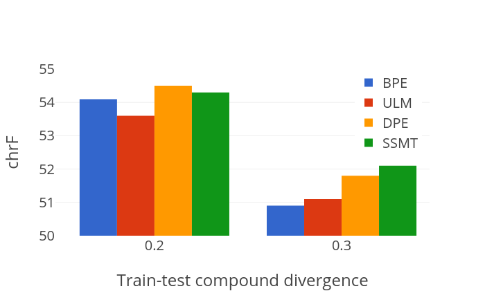
Figure 3: MT performance of our English $\rightarrow$ Zulu models on test subsets that are easier (left) and harder (right) in terms of morphological compositional generalisation.

8 Conclusion

SSMT unifies subword segmentation, MT training, and decoding in a single model. Our results show that it improves translation over existing segmenters when the target language is agglutinative and conjunctively written. It also produces subwords that are closer to morphemes and learns subword-to-word composition that more closely resembles morphological composition. In future work our dynamic decoding algorithm could be used to generate text with subword segmental models for text generation tasks other than MT.

Limitations

The main downside of SSMT (compared to pre-segmentation models like BPE and ULM) is its computational complexity. Our architecture (Figure 1) introduces additional computation in 2 way. Firstly, the decoder conditions on the character-level history of the target sentence, so it has to process more tokens than a standard subword decoder. Secondly, the dynamic programming algorithm (Equation 5) requires more computations than standard MT models training on pre-segmented datasets. In practice, SSMT takes an order of magnitude ($10\times$) longer to train than models training on a pre-segmented dataset. Dynamic decoding also adds computational complexity to testing, although this is less of an issue since test set sizes usually permit run times within a few hours.

It would depend on the practitioner to decide whether the performance boosts obtained by SSMT justify the longer training and decoding times. However, since SSMT is particularly strong for data scarce translation, the computational complexity might be less of an issue. For translation directions like English to Swati, training times are quite short for all models (less than a day for SSMT on subpartitions of the A100 GPU), so the increased training times are manageable.

	Xhosa			Zulu			Swati
Model	P	R	F1	P	R	F1	P	R	F1
BPE	18.04	14.23	15.91	24.51	17.52	20.43	9.13	3.77	5.33
ULM	31.59	22.51	26.29	31.47	20.88	25.10	32.31	13.72	19.26
DPE	28.82	26.16	27.43	33.01	26.36	29.31	7.97	3.72	5.08
SSMT	31.58	41.50	35.87	33.81	39.57	36.46	27.57	15.49	19.83

Table 6: Morpheme identification performance across all words in the morphologically annotated dataset. Morpheme identification measures how much overlap their is between the subwords in a particular segmentation and the morphemes of a word.

Appendix A Next-character probabilities

Here we present the formulas to compute next-character probabilities with the SSMT mixture model. The probability computations depend on whether the preceding character and next character continue or end subwords, so we provide definitions for all possible subword boundary conditions. We consider the simplest case first. Given that the previously generated character at position $j-1$ concludes a subword, the probability of the next subword being a single character $y$ is

$$p_{\text{end-end}}(y|\mathbf{y_{<j}},\mathbf{x})=\,\, g_{j}p_{\mathrm{char}}(y,\textrm{<eos>}\,|\,\mathbf{y_{<j}},\mathbf{x})+$$

$$(1-g_{j})p_{\mathrm{lex}}(y|\mathbf{y_{<j}},\mathbf{x}),$$ (6)

where <eos> is a special end-of-subword token. We can compute this for all $y$ in the character vocabulary and return the top candidates for next character. We modify this for the case where character $j-1$ does not conclude a subword, but character $j$ still does. Then character $j$ constitutes the last character in a subword that started at an earlier character. The probability of next character is then

$$\mkern-30.0mup_{\text{con-end}}(y|\mathbf{y_{<j}},\mathbf{x})$$

$$\mkern-30.0mu=\,\,g_{j}p_{\mathrm{char}}(y,\textrm{<eos>}\,|\,\mathbf{y_{k:j-1}},\mathbf{y_{<k}},\mathbf{x})+$$

$$\,\,\,\,\,\,\,\,\,(1-g_{j})p_{\mathrm{lex}}(y|\mathbf{y_{k:j-1}},\mathbf{y_{<k}},\mathbf{x}),$$ (7)

where $k$ is the starting position of the current subword (concluding at $j$) and $\mathbf{y_{k:j-1}}$ are the characters generated so far in the current subword.

These cases still only give us candidates for when the next character concludes a subword. We can modify equation A to compute the probability of the next character starting and continuing a subword as

$$p_{\text{end-con}}(y|\mathbf{y_{<j}}, \mathbf{x})=\,\,g_{j}p_{\mathrm{char}}(y|\mathbf{y_{<j}},\mathbf{x})+$$ (8)

$$(1-g_{j})\sum_{\mathbf{s}:s_{1}=y,\mathbf{s}\neq y}p_{\mathrm{lex}}(\mathbf{s}|\mathbf{y_{<j}},\mathbf{x}).$$

where the first mixture component is simply the probability of the next character under the character-level model (without the <eos> token). The second component marginalises over all subwords starting with $y$. This considers all the possible ways in which the next subword could start with character $y$. It excludes the 1-character subword $y$ ($\mathbf{s}\neq y$), since this constitutes a subword ending with character $j$ (covered by equation A). Like equation A, this covers the case in which the previous character concludes a subword. Similarly to how we generalised equation A to equation A, we can generalise equation 8 to the case where character $j$ continues a subword started at any given previous character. This produces

$$p {}_{\text{con-con}}(y|\mathbf{y_{<j}},\mathbf{x})=\,\,g_{j}p_{\mathrm{char}}(y|\,\mathbf{y_{k:j-1}},\mathbf{y_{<k}},\mathbf{x})+$$

$$(1-g_{j})\sum_{\mathbf{s}:s_{1}=y,\mathbf{s}\neq y}p_{\mathrm{lex}}(\mathbf{s}|\,\mathbf{y_{k:j-1}},\mathbf{y_{<k}},\mathbf{x}).$$ (9)

Appendix B Training details

SSMT is implemented as a sequence-to-sequence model in the fairseq library. For all our MT models we used the training hyperparameters of the fairseq transformer-base architecture (6 encoder layers, 6 decoder layers). We extensively tuned the vocabulary sizes of our models on both English-Xhosa and English-Zulu (including separate vocabularies). Validation performance peaked for both at a shared vocabulary of 10k subwords for the baselines. For SSMT it peaked at 5k BPE subwords for the source language and 5k subwords in the target language lexicon. We applied these vocabulary settings to the remaining languages (excluding Swati, which we tuned separately).

Our SSMT subwords have a maximum segment length of 5 characters, since this was computationally feasible and validation performance did not improve with longer subwords. We trained all our models for 25 epochs initially and then continued training until validation performance stopped improving for 5 epochs. We trained our DPE segmentation models for 20 epochs (following He et al. (2020)), so DPE required 20 epochs of training for the segmentation model, followed by 25+ epochs for the translation model. We tried sampling ULM segmentations during training for regularisatiion, but initial experiments showed that maximising segmentations led to better validation performance.

Since models are more sensitive to hyperparameter settings in the data scarce setting (Araabi and Monz, 2020), we performed more extensive hyperparameter tuning for the extremely low-resource case of English $\rightarrow$ Swati. We tuned the number of layers and the vocabulary size (see Figure 4). We found that smaller models (less layers) greatly improved validation performance for all models.

	Mixture beam search		Dynamic decoding
Beam size	BLEU	chrF	BLEU	chrF
1	11.8	49.7	13.6	52.2
3	11.5	49.2	14.1	53.6
5	11.2	49.4	14.5	53.8
7	11.4	49.6	14.3	53.8
10	11.5	49.8	14.4	53.8

Table 7: English $\rightarrow$ Zulu validation set performance of SSMT with dynamic decoding compared to standard beam search over the lexicon and character distributions of the SSMT mixture model. Applying standard beam search to SSMT results in poor performance, which justifies the introduction and added computational complexity of dynamic decoding.

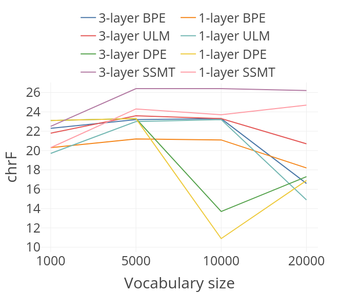
Figure 4: English $\rightarrow$ Swati validation performance.

Motivation

Practical Cognitive Intrinsic Fairness ☑ ☑

Generalisation type

Compositional Structural Cross-task Cross-language Cross-domain Robustness ☑ ☑

Shift type

Covariate Label Full Assumed ☑

Shift source

Naturally occuring Partitioned natural Generated shift Fully generated ☑

Shift locus

Train–test Finetune train–test Pretrain–train Pretrain–test ☑

Table 8: GenBench evaluation card (https://genbench.org/) categorising our morphological compositionl generalisation experiment according to the generalisation taxonomy of Hupkes et al. (2022).

Appendix C Morphological compositional generalisation test subset extraction

For a train set $V$ and test set $W$ we compute the compound divergence and atom divergence, respectively as

$$\mathcal{D}_{C}(V||W)=1-C_{0.1}(F_{C}(V)||F_{C}(W)),$$ (10)

$$\mathcal{D}_{A}(V||W)=1-C_{0.5}(F_{A}(V)||F_{A}(W)),$$ (11)

where $C_{\alpha}(P||Q)$ is the Chernoff coefficient (Chung et al., 1989). This is a measure of the similarity of 2 distributions $P$ and $Q$ computed as

$$C_{\alpha}(P||Q)=\sum_{k}p_{k}^{\alpha}q_{k}^{1-\alpha},$$ (12)

where $\alpha$ is a parameter that weights the importance of the distributions in the similarity metric. We follow Keysers et al. (2020) in setting $\alpha=0.1$ for compound divergence (more important to measure whether or not compounds occur in train than to measure how close the distributions are) and $\alpha=0.5$ for atom divergence (atom distributions should match as far as possible).

We implement a procedure that, given a train set $V$, extracts a prespecified number of sentences from a test set $W$, such that $\mathcal{D}_{C}(V||W)=\mathcal{D}_{C}^{\mathrm{target}}$ (where $\mathcal{D}_{C}^{\mathrm{target}}$ is the desired compound divergence) and $\mathcal{D}_{A}(V||W)$ is held as low as possible. The procedure starts with the empty test subset and iteratively adds one sentence from the test set. At each step, it randomly samples $k$ sentences from the test set (we set $k=100$) and adds the sentence that minimises

$$|\mathcal{D}_{C}-\mathcal{D}_{C}^{\mathrm{target}}|+\mathcal{D}_{A},$$ (13)

where $\mathcal{D}_{C}^{\mathrm{target}}$ is the prespecified compound divergence target for the experiment. Iteratively adding sentences that minimise equation 13 results in a test subset containing atoms (morphemes) that the model was exposed to during training, but compounds (words) that it was not. We can control the degree of compositional novelty in the test subset compounds by setting $\mathcal{D}_{C}^{\mathrm{target}}$ in our procedure.

References

- Araabi and Monz (2020) Ali Araabi and Christof Monz. 2020. Optimizing transformer for low-resource neural machine translation. In Proceedings of the 28th International Conference on Computational Linguistics, pages 3429–3435, Barcelona, Spain (Online). International Committee on Computational Linguistics.
- Bapna et al. (2022) Ankur Bapna, Isaac Caswell, Julia Kreutzer, Orhan Firat, Daan van Esch, Aditya Siddhant, Mengmeng Niu, Pallavi Nikhil Baljekar, Xavier Garcia, Wolfgang Macherey, Theresa Breiner, Vera Saldinger Axelrod, Jason Riesa, Yuan Cao, Mia Chen, Klaus Macherey, Maxim Krikun, Pidong Wang, Alexander Gutkin, Apu Shah, Yanping Huang, Zhifeng Chen, Yonghui Wu, and Macduff Richard Hughes. 2022. Building machine translation systems for the next thousand languages. Technical report, Google Research.
- Chung et al. (1989) J.K Chung, P.L Kannappan, C.T Ng, and P.K Sahoo. 1989. Measures of distance between probability distributions. Journal of Mathematical Analysis and Applications, 138(1):280–292.
- Clark et al. (2022) Jonathan H. Clark, Dan Garrette, Iulia Turc, and John Wieting. 2022. Canine: Pre-training an efficient tokenization-free encoder for language representation. Transactions of the Association for Computational Linguistics, 10:73–91.
- Downey et al. (2021) C. M. Downey, Fei Xia, Gina-Anne Levow, and Shane Steinert-Threlkeld. 2021. A masked segmental language model for unsupervised natural language segmentation. arXiv:2104.07829.
- Edman et al. (2022) Lukas Edman, Antonio Toral, and Gertjan van Noord. 2022. Subword-delimited downsampling for better character-level translation.
- Fodor and Pylyshyn (1988) Jerry A. Fodor and Zenon W. Pylyshyn. 1988. Connectionism and cognitive architecture: A critical analysis. Cognition, 28(1):3–71.
- Gage (1994) Philip Gage. 1994. A new algorithm for data compression. C Users J., 12(2):23–38.
- Gaustad and Puttkammer (2022) Tanja Gaustad and Martin J. Puttkammer. 2022. Linguistically annotated dataset for four official south african languages with a conjunctive orthography: Isindebele, isixhosa, isizulu, and siswati. Data in Brief, 41:107994.
- He et al. (2020) Xuanli He, Gholamreza Haffari, and Mohammad Norouzi. 2020. Dynamic programming encoding for subword segmentation in neural machine translation. In Proceedings of the 58th Annual Meeting of the Association for Computational Linguistics, pages 3042–3051, Online. Association for Computational Linguistics.
- Hupkes et al. (2020) Dieuwke Hupkes, Verna Dankers, Mathijs Mul, and Elia Bruni. 2020. Compositionality decomposed: How do neural networks generalise? (extended abstract). In Proceedings of the Twenty-Ninth International Joint Conference on Artificial Intelligence, IJCAI-20, pages 5065–5069. International Joint Conferences on Artificial Intelligence Organization. Journal track.
- Hupkes et al. (2022) Dieuwke Hupkes, Mario Giulianelli, Verna Dankers, Mikel Artetxe, Yanai Elazar, Tiago Pimentel, Christos Christodoulopoulos, Karim Lasri, Naomi Saphra, Arabella Sinclair, Dennis Ulmer, Florian Schottmann, Khuyagbaatar Batsuren, Kaiser Sun, Koustuv Sinha, Leila Khalatbari, Maria Ryskina, Rita Frieske, Ryan Cotterell, and Zhijing Jin. 2022. State-of-the-art generalisation research in NLP: a taxonomy and review. CoRR.
- Kawakami et al. (2019) Kazuya Kawakami, Chris Dyer, and Phil Blunsom. 2019. Learning to discover, ground and use words with segmental neural language models. In Proceedings of the 57th Annual Meeting of the Association for Computational Linguistics, pages 6429–6441, Florence, Italy. Association for Computational Linguistics.
- Keysers et al. (2020) Daniel Keysers, Nathanael Schärli, Nathan Scales, Hylke Buisman, Daniel Furrer, Sergii Kashubin, Nikola Momchev, Danila Sinopalnikov, Lukasz Stafiniak, Tibor Tihon, Dmitry Tsarkov, Xiao Wang, Marc van Zee, and Olivier Bousquet. 2020. Measuring compositional generalization: A comprehensive method on realistic data. In International Conference on Learning Representations.
- Kim and Linzen (2020) Najoung Kim and Tal Linzen. 2020. COGS: A compositional generalization challenge based on semantic interpretation. In Proceedings of the 2020 Conference on Empirical Methods in Natural Language Processing (EMNLP), pages 9087–9105, Online. Association for Computational Linguistics.
- Klein and Tsarfaty (2020) Stav Klein and Reut Tsarfaty. 2020. Getting the ##life out of living: How adequate are word-pieces for modelling complex morphology? In Proceedings of the 17th SIGMORPHON Workshop on Computational Research in Phonetics, Phonology, and Morphology, pages 204–209, Online. Association for Computational Linguistics.
- Koehn (2004) Philipp Koehn. 2004. Statistical significance tests for machine translation evaluation. In Proceedings of the 2004 Conference on Empirical Methods in Natural Language Processing, pages 388–395, Barcelona, Spain. Association for Computational Linguistics.
- Kong et al. (2016) Lingpeng Kong, Chris Dyer, and Noah A. Smith. 2016. Segmental recurrent neural networks. In 4th International Conference on Learning Representations, ICLR 2016, San Juan, Puerto Rico, May 2-4, 2016, Conference Track Proceedings.
- Kreutzer and Sokolov (2018) Julia Kreutzer and Artem Sokolov. 2018. Learning to segment inputs for NMT favors character-level processing. In Proceedings of the 15th International Conference on Spoken Language Translation, pages 166–172, Brussels. International Conference on Spoken Language Translation.
- Kudo (2018) Taku Kudo. 2018. Subword regularization: Improving neural network translation models with multiple subword candidates. In Proceedings of the 56th Annual Meeting of the Association for Computational Linguistics (Volume 1: Long Papers), pages 66–75, Melbourne, Australia. Association for Computational Linguistics.
- Lake and Baroni (2018) Brenden M. Lake and Marco Baroni. 2018. Generalization without systematicity: On the compositional skills of sequence-to-sequence recurrent networks. In International Conference on Machine Learning.
- Libovický et al. (2022) Jindřich Libovický, Helmut Schmid, and Alexander Fraser. 2022. Why don’t people use character-level machine translation? In Findings of the Association for Computational Linguistics: ACL 2022, pages 2470–2485, Dublin, Ireland. Association for Computational Linguistics.
- Meyer and Buys (2022) Francois Meyer and Jan Buys. 2022. Subword segmental language modelling for nguni languages. arXiv:2210.06525.
- Moeng et al. (2021) Tumi Moeng, Sheldon Reay, Aaron Daniels, and Jan Buys. 2021. Canonical and surface morphological segmentation for nguni languages. In Proceedings of the Second Southern African Conference for Artificial Intelligence Research (SACAIR), pages 125–139, Online. Springer.
- Partee (1984) Barbara Partee. 1984. Compositionality. Varieties of formal semantics, 3:281––311.
- Popović (2015) Maja Popović. 2015. chrF: character n-gram F-score for automatic MT evaluation. In Proceedings of the Tenth Workshop on Statistical Machine Translation, pages 392–395, Lisbon, Portugal. Association for Computational Linguistics.
- Sennrich et al. (2016) Rico Sennrich, Barry Haddow, and Alexandra Birch. 2016. Neural machine translation of rare words with subword units. In Proceedings of the 54th Annual Meeting of the Association for Computational Linguistics (Volume 1: Long Papers), pages 1715–1725, Berlin, Germany. Association for Computational Linguistics.
- Sun and Deng (2018) Zhiqing Sun and Zhi-Hong Deng. 2018. Unsupervised neural word segmentation for Chinese via segmental language modeling. In Proceedings of the 2018 Conference on Empirical Methods in Natural Language Processing, pages 4915–4920, Brussels, Belgium. Association for Computational Linguistics.
- Tay et al. (2022) Yi Tay, Vinh Q. Tran, Sebastian Ruder, Jai Gupta, Hyung Won Chung, Dara Bahri, Zhen Qin, Simon Baumgartner, Cong Yu, and Donald Metzler. 2022. Charformer: Fast character transformers via gradient-based subword tokenization. In International Conference on Learning Representations.
- Wang et al. (2017) Chong Wang, Yining Wang, Po-Sen Huang, Abdelrahman Mohamed, Dengyong Zhou, and Li Deng. 2017. Sequence modeling via segmentations. In Proceedings of the 34th International Conference on Machine Learning - Volume 70, page 3674–3683. JMLR.org.
- Wang et al. (2021) Xinyi Wang, Sebastian Ruder, and Graham Neubig. 2021. Multi-view subword regularization. In Proceedings of the 2021 Conference of the North American Chapter of the Association for Computational Linguistics: Human Language Technologies, pages 473–482, Online. Association for Computational Linguistics.
- Yu et al. (2016) Lei Yu, Jan Buys, and Phil Blunsom. 2016. Online segment to segment neural transduction. In Proceedings of the 2016 Conference on Empirical Methods in Natural Language Processing, pages 1307–1316, Austin, Texas. Association for Computational Linguistics.
- Zhu et al. (2019) Yi Zhu, Benjamin Heinzerling, Ivan Vulić, Michael Strube, Roi Reichart, and Anna Korhonen. 2019. On the importance of subword information for morphological tasks in truly low-resource languages. In Proceedings of the 23rd Conference on Computational Natural Language Learning (CoNLL), pages 216–226, Hong Kong, China. Association for Computational Linguistics.
- Ács (2019) Judit Ács. 2019. Exploring bert’s vocabulary.