Energy-preserving Indirect-feedback for Wireless Power Transfer

Abstract

Recognising the limitations of various existing channel-estimation schemes for energy beamforming, we propose an energy-preserving indirect feedback-based approach for finding the optimal beamforming vector. Upon elaborating on the key ideas behind the proposed approach—dynamics of the harvest-then-transmit protocol and the latency associated with the charging process—we present an algorithm and its hardware architecture to concretise the proposed approach. The algorithm and the hardware architecture are supplemented by mathematical analysis, numerical simulation and hardware utilisation details, ASIC synthesis and post-layout simulation details, respectively. We firmly believe this paper, due to its unified algorithm-hardware design, will open up new avenues for research in radio frequency (RF) wireless power transfer.

I Introduction

Wireless power transfer (WPT) through radio frequency (RF) signals has been envisaged as one of the key drivers for the mass adoption of the internet-of-things (IoT). The benefits of the WPT over the conventional power delivery method, i.e., employing batteries, are several, such as reduction in the weight of devices, curtailment of the maintenance cost, and relief from the tiresome routine of replacing or recharging on-device batteries. Additionally, the WPT is eco-friendly as it curbs e-waste generation by alleviating the usage of batteries. The adoption of WPT will usher in the era of true mobility as both information and power will be delivered wirelessly. However, there are several technological challenges to transform the WPT from a promising technology to full-fledged solution for powering the next generation IoT systems. Hence, such challenges must be addressed foremost to proliferate the deployment of WPT.

The WPT has been plagued by its low end-to-end energy transfer efficiency since its inception. Primarily, this is attributed to the omnidirectionality of the electromagnetic radiation from standard radiative elements, e.g., dipole antennas. To address this issue, energy beamforming with the help of a multi-antenna transmitter has been reported in literature [1], where the electromagnetic energy radiated by an antenna array is focused in a direction by adjusting gains and phases of individual antenna elements. However, to perform energy beamforming, a transmitter must estimate the channel between itself and a receiver by enrolling help from the receiver, leading to additional challenges, especially when the receiver is under stringent power constraints.

The necessity of estimating downlink wireless channels is already well-motivated in the multi-antenna, single as well as multi-user wireless communication scenarios. As a result, various estimation schemes had been proposed in the wireless communication literature. Systems adopting time division duplexing (TDD) estimate the downlink channel with the help of uplink pilot tones by exploiting the channel reciprocity. On the other side, when frequency division duplexing (FDD) is employed, downlink pilots and the feedback from the receivers are essential for reliable estimates.

It is apparent that both the aforementioned techniques require the active participation of receivers, and consequently, incorporating any of them into energy harvesting devices will cost a portion of the harvested energy. Subsequently, the depletion of harvested energy will lessen the throughput when the harvesting device transmits its information. The pilot-based schemes are also ill-suited for the scenarios where the information and energy transmission are scheduled in different frequency bands. This is because the reciprocity assumption is hardly valid in such cases, especially when those bands are far apart in the frequency spectrum or differ in bandwidth. Recognizing the limitation of the conventional channel estimation schemes concerning the wireless power transfer, we ask a question, “Is it possible to find the optimal beamforming vector for energy beamforming without costing any energy at the energy harvester?”.

We attempt to answer this question by delving inside the charging subsystem of a generic energy harvester device, often treated as a black box in the wireless communication literature. Furthermore, we exploit the temporal dependency of the information transmission on the energy harvesting process imposed by the prevalent harvest-then-transmit protocol [1]. The dynamics of the harvest-then-transmit protocol, combined with the inherent delay present in the charging process, facilitate a unique way of obtaining feedback regarding the channel state information or a chosen beamforming vector. Yet, such unprecedented approach has not been adopted in the literature.

Compared to several iterative single or multi-bit feedback schemes [2, 3] proposed in the literature, the approach presented here is energy-preserving as it relies on indirect feedback. The energy saved in this manner can be utilised in information processing, reception or transmission at the energy harvesting device, resulting in the superior performance of energy harvesting systems.

For ease of reference, we list the major contribution of this article below.

• We first propose a scheme to find the optimal beamforming vector for a multiple-input single-output (MISO) wireless power transfer set up where no explicit participation, e.g., the transmission of pilot signals or direct feedback regarding the pilots transmitted by the energy transmitter, is needed at the energy receiver end. We also elaborate on the proposed scheme with the help of a schematic representation of the overall system.

• We present an algorithm to find the optimal beamforming vector from the time-to-recharge values of probing vectors obtained from an orthonormal basis of $\mathbb{C}^{N}$, where $N$ is the number of antennas at the transmitter. By recognising the limitation of the proposed algorithm, we suggest modifications in the algorithm that results in curtailment of the probing duration (referred to as FAP phase in section III).

• In order to facilitate the rapid deployment of our proposed solution in contemporary wireless devices/systems, this paper also present a new digital hardware architecture for the proposed optimal beamforming vector finding algorithm. To the best of the authors’ knowledge, such a digital architecture is the first-time implementation in the WPT literature. Its micro-architecture design and hardware implementation results have been comprehensively presented here. The notion of such a hybrid design process is to shed ample information towards fine-tuning various design parameters of the proposed energy beamforming solution that leads to a superior and practical design suitable for real-world applications.

Organisation

Section II lists various related works from where the current article has drawn inspiration and highlights the research gap addressed in this paper. In section III, we elaborate on the system model considered in this paper. Two major contributions of this paper, namely, the algorithm to find the optimal beamforming vector and a digital hardware architecture for the same are presented in the sections IV and V, respectively. We present numerical results in section VI to demonstrate the performance of the proposed algorithm with respect to various system parameters. Lastly, we conclude the paper in the section VII by reiterating and summarising the major contributions of this paper.

Notation

We denote vectors and matrices using lower-case and upper-case boldface fonts, respectively. $\mathbf{a}^{\dagger}$ represents complex conjugate transpose of a complex vector $\mathbf{a}$. Euclidean norm of a vector is denoted by $||.||$. $\mathbb{C}$ denotes the set of complex numbers, and $j$ is the complex number $\sqrt{-1}$. The magnitude, real and imaginary part of a complex number is denoted by $|.|$, $\Re\{.\}$ and $\Im\{.\}$, respectively.

II Related work

As the early works on energy harvesting focused on establishing performance bounds, e.g., achievable throughput [1] and rate-energy trade-offs [4, 5], various issues pertaining to the actual implementations were either overlooked or superficially addressed. The predominantly adopted assumptions, such as availability of the channel state information, and linearity of the energy harvesting circuit, were relaxed in the later years, leading to a more realistic system model and refinement of the performance bounds presented earlier [6, 7]. The study of system models encompassing multi-antenna transmitters underwent a similar transition. While the focus of those studies remained the same—finding an optimal beamforming vector to optimize the utility under consideration—the complexity of resource allocation problems increased manifold due to the introduction of various practical constraints. In the next paragraph, we list a few notable works to highlight the importance of the availability of channel state information for optimizing throughput or transmit power or received power for multi-antenna WPT or simultaneous wireless information and power transfer (SWIPT) systems. In the subsequent paragraphs, we review different channel estimation schemes for multi-antenna WPT proposed in the literature and a few works that delve into the hardware architecture of their proposed strategies to position our work in the research landscape concerning wireless power transmission and harvesting.

Throughput maximization for multi-antenna wireless power transfer systems studied in [8] was later revisited in [7] by relaxing the full CSI requirement and adopting a non-linear energy harvesting model. Maximizing the (weighted) sum received power at energy receivers was the objective of the studies carried out in [9] and [10], with the latter extending the analysis to the imperfect CSI case. On the other hand, the authors in [11] and [12] targeted the transmit power minimization problem for a single transmitter multi-user MISO SWIPT scenario and MISO interference channel with K transmitter-receiver pairs, respectively. The interference caused by signals intended for other receivers was mitigated by jointly optimizing the beamforming vector at transmitter(s) and power-splitting ratios at each mobile station.

Various approaches proposed in the literature for downlink channel estimation in WPT are nonetheless minor variations of their counterparts in wireless communication. Hence, many disregarded the differences between wireless communication and WPT systems. For example, WPT is unidirectional, unlike the data communication in wireless communications, and therefore, requires relatively simpler hardware for implementation than the latter. Additionally, if energy harvesting devices solely rely on the harvested energy for their operations, transmitting pilot or feedback signals for them could be burdening, if not practically realisable. Nevertheless, the schemes employing uplink pilot [13, 14] and received-power feedback [15, 16, 17, 18, 19, 20] provide frameworks for developing improved channel estimation schemes and benchmarking them.

The transmitter side operations of our proposed scheme are similar to the received-power feedback-based schemes. However, the receiver side differs significantly in design as well as operations. In the received-power feedback schemes, a receiver measures the received power or energy, possibly with an energy meter [2], over an interval and feedback a quantized value of the measured power or difference of the measured power over two consecutive intervals to the transmitter [19]. However, the quantization can be skipped if the transmitter refers to a pre-shared codebook for choosing a beamforming vector and the receiver feedback the code corresponding to the beamforming vector that resulted in the maximum received power [3]. Two apparent shortcomings of the received-power feedback-based schemes are addressed in our proposed approach that exploits the dynamics of the harvest-then-transmit protocol. The first shortcoming is the requirement of an additional feedback module comprising an energy meter, quantizer, and additional RF components (if the feedback is sent over a different channel). The second one is the direct dependency of the channel estimation accuracy on the nature of feedback (partial/full) [15] or the number of feedback bits [19]. As the feedback considered in our work is indirect and the instrumentation for processing the feedback is part of the transmitter, the two shortcomings mentioned above are tackled.

The indirect feedback-based approaches, also termed blind or hidden feedback, appeared in wireless communication literature in the context of cognitive radio [21, 22]. In [21], the primary transmitter’s power adaption acts as indirect feedback to the secondary users, which is employed to reduce the interference caused to the primary receivers by the secondary transmitters. A similar approach was proposed in [22] to find the null space of the MIMO channel between the secondary transmitter and the primary receiver for an underlay cognitive radio network. However, to the best of our knowledge, finding the optimal beamforming vector for WPT by employing indirect feedback has not appeared in the literature.

Hardware implementation aspect of WPT systems has been sparsely reported in the literature. Recently, Samith et al. demonstrated the system-level hardware implementation in [18, 20] that enables energy beamforming by using received signal strength indicator (RSSI) value for the channel estimation. Here, the experimental validation has been carried out with the aid of USRPs and commercially available ultra-low power microcontrollers. In [23], hardware validation of wireless energy transfer to the onboard (P1110 evaluation board) energy storage element has been demonstrated with the aid of a dedicated RF energy source in conjunction with 6.1 dBi antenna. To the best of authors’ knowledge, dedicated digital hardware-architecture suitable for field-programmable gate-array (FPGA) and application-specific integrated-circuits (ASIC) implementation platforms for any indirect feedback-based energy beamforming is unexplored till date. Hence, by proposing a generic and new digital architecture for the same this work will play key role in the development of hardware- and energy-efficient WPT systems. Aforementioned holistic approach of designing a new algorithm and its corresponding architecture is an absolute necessity for transforming an unprecedented idea into real-world implementation. Such contributions are widely adopted by various state-of-the-art implementations [24, 25].

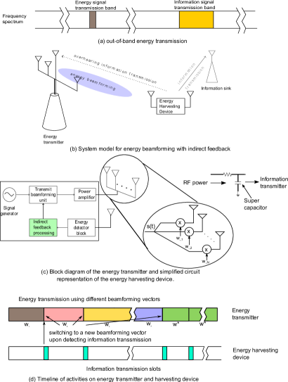
Figure 1: A system level overview of the indirect feedback based energy beamforming scheme.

III System model

The system model considered in this article is similar to the one mentioned in [18, 20, 26], where a multi-antenna energy transmitter transfers energy via RF signals to a single antenna energy harvester by employing energy beamforming. However, unlike [20], we assume an out-of-band separated receiver architecture, i.e., energy harvester and information transceiver have different antennas and RF blocks and they operate on different frequency bands [27] (refer to Fig. 1(a)). There are two major reasons for considering this architecture. First, decoupling the energy harvesting, and information transmission processes and the associated hardware becomes feasible—a prerequisite for our indirect feedback-based energy beamforming scheme. Second, it has been adopted in commercial products, e.g., Powercast energy harvesters [28], an evaluation board predominantly used in the literature to validate various theoretical findings.

Specifically, in our system model, we assume that the energy transmitter has $N$ antennas supported by the associated hardware for energy transmission and one dedicated antenna backed by an information processing unit for overhearing the (information) transmission of the energy harvester device. On the other hand, the energy harvester is equipped with two antennas and associated RF blocks— one for energy reception and the other for communication. Additionally, we assume that the channel between the transmitter and receiver varies slowly due to their proximity and immobility.

The block diagram of our system model, shown in Fig. 1(b), depicts an energy transmitter with two sets of antennas, an energy receiver (information transmitter) and an information sink along with the directions of energy transmission, information transmission and indirect feedback. In Fig. 1(c), we present a schematic overview of the internal blocks of the energy transmitter.

III-A Signals transmitted and received

We assume that the energy transmitter generates a single tone signal, $s(t)=\sqrt{2}\cos(2\pi f_{c}t)$, having frequency $f_{c}$, and multiplies it with a unit-norm beamforming vector $\mathbf{w}\in\mathbb{C}^{N}$. Following that, it transmits the signal through antennas after amplifying them by a set of power amplifiers whose amplification factor is governed by the transmit power ($P_{t}$) of the energy transmitter. Note that though we are considering a narrow-band (single tone) signal, the proposed algorithm can be applied to wideband signals, e.g., multi-tone signals [29], with little or no changes.

We express the transmitted signal from the energy transmitter as

$$\mathbf{y}(t)=\sqrt{P_{t}}\mathbf{w}s(t).$$ (1)

Assuming that the channel gain between the transmitter and the energy harvester is denoted by a complex vector $\mathbf{h}\in\mathbb{C}^{N}$, we write the received signal at the energy harvester as

$$r(t)=\sqrt{GP_{t}}\mathbf{h}^{\dagger}\mathbf{w}s(t),$$ (2)

where the constant $G$ captures the effect of antenna gain, polarization, and wavelength of the transmitted signal, etc. on the received signal [30]. The average received power at the harvester is obtained by averaging the absolute square of the received signal over a sufficiently long interval and can be expressed as

$$P_{r}=GP_{t}|\mathbf{h}^{\dagger}\mathbf{w}|^{2}.$$ (3)

From (3) it is apparent that for a given transmitter-receiver set up (i.e., for a fixed $G$) and transmit power, the received power will be maximized if the beamforming vector ($\mathbf{w}$) is chosen in such a way that $|\mathbf{h}^{\dagger}\mathbf{w}|$ is maximized. As $\mathbf{w}$ is assumed to be a unit-norm vector, it can be easily shown that $\mathbf{w}=\mathbf{h}e^{j\theta}/||\mathbf{h}||$ with an arbitrary $\theta$ is the desired beamforming vector.

III-B Energy harvester model

Now we focus on the energy harvester and explain the harvesting process. The received signal is a single-tone RF signal, possibly, distorted by the non-linearities present in the RF reception block of the energy harvester. This signal is rectified and filtered to produce a DC signal suitable for charging a super-capacitor.

The RF-to-DC conversion efficiency, also referred to as harvesting efficiency, is the ratio of the powers of the received RF and the output DC signals. As the rectifier circuit comprises various non-linear components, e.g., diode and transistors, the nonlinearity of the harvesting efficiency is evident. Therefore, an accurate characterisation of the performance of energy harvesting systems requires one to incorporate this non-linearity in system models, which was neglected in several early works. In this work, we assume that the harvesting efficiency belongs to a class of non-negative, non-linear functions defined over an interval of positive real numbers.

Non-linear harvesting efficiency

The harvesting efficiency, denoted as $\eta(\centerdot)$, is a function of the received power, as established in the energy harvesting circuit literature [31]. As a result, the harvested power, $P_{h}$ is related to the received power $P_{r}$ through the following equation

$$P_{h}=\eta(P_{r})P_{r}.$$ (4)

The indirect feedback scheme proposed in this article requires the harvested power to be a monotonic function of the received power, i.e., $dP_{h}/dP_{r}>0$. In other words, if $P_{r_{1}}$, $P_{r_{2}}$ are two received power values, and $P_{h_{1}}$, $P_{h_{2}}$ are corresponding harvesting power values, respectively, then $P_{h_{1}}<P_{h_{2}}$ if and only if, $P_{r_{1}}<P_{r_{2}}$. It is apparent that if $\eta(\centerdot)$ is a constant or a non-decreasing function of $P_{r}$, the above requirement is easily satisfied. Further, one can easily verify various model considered in the literature for estimating harvested power from the received power, e.g., piece-wise linear [32, 33, 34], normalised sigmoid function [7] and the rational function [35], meet the required criterion in their respective non-saturation region. A comparison of some of these models is depicted in Fig. 2.

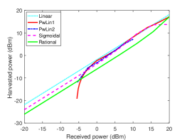
Figure 2: Comparison of various harvesting efficiency models. The first two piece-wise linear models, abbreviated as ‘PwLin’, are reproduced from [32, 34]. The normalised sigmoidal and the rational models from [7, 35], respectively are plotted along with the linear ($\eta=0.7$) model.

Constant power source and energy storage

A super-capacitor acting as energy storage accumulates electric charge from the signal processed by the rectifier-filter block. In practical harvesting systems, multi-stage charge pump circuits, e.g., Cockcroft-Walton or Dickson charge pumps [31], or boost converters precede the energy storage block for the improved charge delivery. However, similar to [36], we model the energy storage as a series R-C circuit for ease of exposition (refer to Fig. 1(c)). Further, we assume that the output of the rectifier block acts as a constant power source, proposed and validated in [23], and drives the R-C circuit.

Time-to-recharge

The constant power source R-C circuit based energy storage system was considered in [34] to obtain a closed-form expression for the time-to-recharge of an energy harvester. It was shown that the time-to-recharge of an energy harvester for a fixed received power (at the input of the R-C circuit) is

$$\!t_{tr}(q_{m},q_{0},P_{h})\!=\!\frac{RC}{2}\!\ln\!\left(\frac{Y(q_{m},P_{h})\exp(Y(q_{m},P_{h}))}{Y(q_{0},P_{h})\exp(Y(q_{0},P_{h}))}\right),$$ (5)

where $Y(q,P)=\frac{(q+\sqrt{q^{2}+4PRC^{2}})^{2}}{4PRC^{2}}$, $P_{h}$ is the input power to the R-C circuit, $R$ and $C$ denote the resistance and capacitance of the series R-C (energy storage) circuit, and $q_{0},q_{m}$ are the initial and desired charge levels, respectively. Intuitively, a larger value of $P_{h}$ will result in a smaller $t_{tr}$ and the same can be seen from Fig. 3 as well.

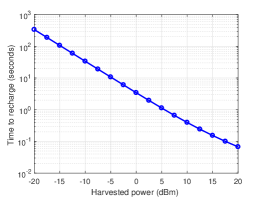
Figure 3: Time-to-recharge vs harvested power obtained from (5) by considering $R=100\Omega$, $C=1$mF, $q_{0}=1.5$ milli Coulombs, and $q_{m}=3$ mC.

Indirect feedback from the time-to-recharge

From (3) and (4), we identify the relation between a beamforming vector and the resultant harvested power. By expressing the harvested power as a function of the beamforming vector, for given $q_{0},q_{m}$, we obtain the following functional relation between the time-to-recharge and the corresponding beamforming vector from (5)

$$t_{tr-bm}(\mathbf{w})=t_{tr}(q_{m},q_{0},P_{h}(\mathbf{w}))=f_{ttr}(|\mathbf{h}^{\dagger}\mathbf{w}|).$$ (6)

The indirect feedback about a beamforming vector is obtained through (6)—the closer a vector is to the instantaneous channel gain in cosine similarity, the smaller the time-to-recharge. Additionally, if (4) is satisfied, we can find the harvested power $P_{h}$ and subsequently, $|\mathbf{h}^{\dagger}\mathbf{w}|$ through an inverse mapping $f_{ttr}^{-1}:\mathbb{R}_{+}\to\mathbb{R}_{+}$, such that

$$f_{ttr}^{-1}(t_{tr-bm})=|\mathbf{h}^{\dagger}\mathbf{w}|.$$ (7)

In the following subsections, we describe how an energy transmitter can obtain indirect feedback about the beamforming vector employed and subsequently improve the power delivery by adopting our proposed algorithm.

III-C Transmission phases and their roles

To capitalize on the indirect feedback received from the energy receiver, we propose dividing the total stretch of energy transmission into two phases: 1) feedback acquisition and processing and 2) energy beamforming transmission, occurring alternately. Fig. 1(d) illustrates the sequencing of these two phases in an ongoing energy transmission-harvesting process. The activities carried out by the energy transmitter and receiver in these phases are briefly described in the following subsections.

Feedback acquisition and processing (FAP)

In this phase, as the name suggests, the energy transmitter acquires (indirect) feedback regarding a set of known beamforming vectors by overhearing the (information) transmissions of the energy harvester. Essentially, the energy transmitter measures the time-to-recharge for these vectors one by one and feeds those measurements to Algorithm 1, described in the following section. The measurement can be done by starting a timer whenever the transmitter employs a new vector and stopping it upon overhearing the energy harvester’s transmission. We are assuming that the measurement taken in this manner is error-free. For ease of illustration, we divide this phase into several slots, each corresponding to a beamforming vector. Needless to say, the duration of these slots will differ as different beamforming vectors are employed in every slot.

Energy beamforming transmission (EBT)

This phase ensues the FAP phase once the optimal beamforming vector is calculated by the Algorithm 1. The optimal beamforming vector is employed to deliver power to the energy harvester in this phase. As the beamforming vector remains unchanged throughout this phase, slotting is not required. However, the energy transmitter continues measuring the time-to-recharge by finding the interval between two consequent information transmissions.

Note that in the proposed indirect feedback scheme, the energy harvester harvests energy from the transmission of the energy transmitter in both phases.

IV Finding the optimal beamforming vector from the indirect feedback

In this section, we present an algorithm that finds the optimal beamforming vector from the feedback collected in the FAP phase. In a nutshell, the proposed algorithm finds the normalized and equally rotated coefficients of the channel gain in an orthonormal basis of $\mathbb{C}^{N}$ from the indirect feedback of the linear combination of vectors from the chosen basis.

Algorithm 1 Algorithm for finding the optimal beamforming vector

0:  $\mathbf{Q},\phi_{1}$, $\phi_{2}$

0:  $\mathbf{w}_{opt}$

1:  Initialization: $\phi_{1}\leftarrow\pi/4$, $\phi_{2}\leftarrow 7\pi/4$.

2:  for $i=1$ to $N$ do

3:     Set $\mathbf{Q}(:,i)$ as beamforming vector and find $\tau_{i}$ from (7)

4:  end for

5:  $\mathbf{w}_{opt}\leftarrow\mathbf{Q}(:,1)$

6:  $dot\_prod\_\mathbf{w}_{opt}\leftarrow\tau_{1}$

7:  for $i=1$ to $N-1$ do

8:     $\alpha_{1}\leftarrow dot\_prod\_\mathbf{w}_{opt}$, $\alpha_{2}\leftarrow\tau_{i+1}$

9:     $\mu\leftarrow\alpha_{1}^{2}+\alpha_{2}^{2}$

10:     $\kappa_{1}\leftarrow(\alpha_{1}^{4}+\alpha_{2}^{4})/\mu$, $\kappa_{2}\leftarrow\alpha_{1}\alpha_{2}/\mu$

11:     $\mathbf{w}_{1}\leftarrow(\alpha_{1}\mathbf{w}_{opt}+e^{j\phi_{1}}\alpha_{2}\mathbf{Q}(:,i+1))/\sqrt{\mu}$

12:     Set $\mathbf{w}_{1}$ as beamforming vector and find $\tilde{\tau}_{1}$

13:     $\mathbf{w}_{2}\leftarrow(\alpha_{1}\mathbf{w}_{opt}+e^{j\phi_{2}}\alpha_{2}\mathbf{Q}(:,i+1))/\sqrt{\mu}$

14:     Set $\mathbf{w}_{2}$ as beamforming vector and find $\tilde{\tau}_{2}$

15:     $\gamma_{R}\leftarrow\frac{\tilde{\tau}_{1}^{2}+\tilde{\tau}_{2}^{2}-2\kappa_{1}}{2\sqrt{2}\kappa_{2}}$, $\gamma_{I}\leftarrow\frac{\tilde{\tau}_{1}^{2}-\tilde{\tau}_{2}^{2}}{2\sqrt{2}\kappa_{2}}$

16:     $\theta_{1}\leftarrow\arctan\left(\frac{-\gamma_{I}}{\gamma_{R}}\right)$, $\theta_{2}\leftarrow\arctan\left(\frac{\gamma_{I}}{-\gamma_{R}}\right)$

17:     if $(\gamma_{R}\cos\theta_{1}-\gamma_{I}\sin\theta_{1})>0$ then

18:        $\mathbf{w}_{opt}\leftarrow(\alpha_{1}\mathbf{w}_{opt}\!+\!e^{j\theta_{1}}\alpha_{2}\mathbf{Q}(:,i\!+\!1))$, $dot\_prod\_\mathbf{w}_{opt}\!\!\leftarrow\!\!\sqrt{\kappa_{1}\!\!+\!\!2\kappa_{2}(\gamma_{R}\cos\theta_{1}\!\!-\!\!\gamma_{I}\sin\theta_{1})}$

19:     else

20:        $\mathbf{w}_{opt}\leftarrow(\alpha_{1}\mathbf{w}_{opt}+e^{j\theta_{2}}\alpha_{2}\mathbf{Q}(:,i+1))$, $dot\_prod\_\mathbf{w}_{opt}\!\!\leftarrow\!\!\sqrt{\kappa_{1}\!\!+\!\!2\kappa_{2}(\gamma_{R}\cos\theta_{2}\!\!-\!\!\gamma_{I}\sin\theta_{2})}$

21:     end if

22:  end for

23:  return  $\mathbf{w}_{opt}$

Assuming that $\{\mathbf{q}_{1},\mathbf{q}_{2},\ldots,\mathbf{q}_{N}\}$ is an ordered orthonormal basis of $\mathbb{C}^{N}$, the unknown channel vector $\mathbf{h}$ can be expressed as

$$\mathbf{h}=\sum\limits_{i=1}^{N}\zeta_{i}\mathbf{q}_{i},\text{ where }\zeta_{i}\in\mathbb{C},\text{ for }i\in\{1,2,\ldots,N\}.$$ (8)

To ease exposition, we collect these basis vectors in a matrix, $\mathbf{Q}$ and refer to them using the column index notation, $\mathbf{Q}(:,i)$. Recalling that $\mathbf{q}_{i}$ is orthogonal to $\mathbf{q}_{j}$, $j\neq i$, one can easily verify that $\mathbf{Q}^{\dagger}\mathbf{h}=\boldsymbol{\zeta}$, where $\boldsymbol{\zeta}=[\zeta_{1},\zeta_{2},\ldots,\zeta_{N}]^{T}$.

When $\mathbf{q}_{i}$ is the beamforming vector, the absolute value of the dot product of the channel gain and the beamforming vector (denoted by $\tau_{i}$ in the Algorithm 1) is

$$|\mathbf{h}^{\dagger}\mathbf{q}_{i}|=\big{|}\big{(}\sum_{k=1}^{N}\zeta_{k}\mathbf{q}_{k}\big{)}^{\dagger}\mathbf{q}_{i}\big{|}=|\zeta_{i}|.$$ (9)

Note that in several conventional channel estimation schemes, $\zeta_{i}$ (its noisy version to be precise) is available at the receiver as the received signal is a linear function of $\mathbf{h}^{\dagger}\mathbf{w}$. Unlike those schemes, the proposed algorithm tries to estimate the channel from the absolute values of $\zeta_{i}$, and therefore, requires additional feedback as well as computation. Consequently, the estimated channel gain is a rotated and scaled version of the actual one, which is sufficient for finding the optimal beamforming vector as pointed out in (3). The optimal beamforming vector produced by the algorithm is

$$\mathbf{w}_{opt}=\sum\limits_{i=1}^{N}\frac{|\zeta_{i}|}{\sqrt{\sum_{i=1}^{N}|\zeta_{i}|^{2}}}\mathbf{q}_{i}e^{j(\angle\zeta_{i}-\angle\zeta_{1})}.$$ (10)

From the above expression, it is apparent that the phase difference between the estimate and the actual channel vector is $\angle\zeta_{1}$.

The proposed algorithm has two for loops—the first one for finding the absolute dot products (cf. (9)), and the second for calculating relative angles (cf. (10)) corresponding to each $\zeta_{i},i=2,\ldots,N$. Once $\tau_{i}(=|\zeta_{i}|)$ are obtained by employing $\mathbf{q}_{i}$ as beamforming vectors in steps 3 - 6, the Algorithm 1 finds the angle between $i$th coefficient and the first one, i.e., $\angle\zeta_{i}-\angle\zeta_{1}$ in an iterative manner. To illustrate this segment (steps 7 - 23) of the algorithm, let us consider the following unit-norm beamforming vector formed by the linear combination of two known unit-norm vectors, $\mathbf{v}_{1},\mathbf{v}_{2}$:

$$\tilde{\mathbf{w}}_{\theta}=\frac{|\mathbf{h}^{\dagger}\mathbf{v}_{1}|\mathbf{v}_{1}+e^{j\theta}|\mathbf{h}^{\dagger}\mathbf{v}_{2}|\mathbf{v}_{2}}{\sqrt{|\mathbf{h}^{\dagger}\mathbf{v}_{1}|^{2}+|\mathbf{h}^{\dagger}\mathbf{v}_{2}|^{2}}}.$$ (11)

In the first iteration, we set $\mathbf{v}_{1}=\mathbf{q}_{1}$, $\mathbf{v}_{2}=\mathbf{q}_{2}$ and generate intermediate unit-norm beamforming vectors of the following form $\tilde{\mathbf{w}}_{\theta}=(|\zeta_{1}|\mathbf{q}_{1}+|\zeta_{2}|e^{j\theta}\mathbf{q}_{2})/(|\zeta_{1}|^{2}+|\zeta_{2}|^{2})$. The numerator of absolute dot product for this beamforming vector can be evaluated as

$$\bigg{|}\big{(}\sum\limits_{i=1}^{N}\zeta_{i}\mathbf{q}_{i}\big{)}^{\dagger}(|\zeta_{1}|\mathbf{q}_{1}+e^{j\theta}|\zeta_{2}|\mathbf{q}_{2})\bigg{|}^{2}$$

$$=\big{|}\zeta_{1}^{*}|\zeta_{1}|+\zeta_{2}^{*}|\zeta_{2}|e^{j\theta}\big{|}^{2}$$

$$=|\zeta_{1}|^{4}+|\zeta_{2}|^{4}+|\zeta_{1}||\zeta_{2}|(\zeta_{1}\zeta_{2}^{*}e^{j\theta}+\zeta_{1}^{*}\zeta_{2}e^{-j\theta})$$ (12)

To find the $\theta$ that maximizes (or minimizes) the absolute dot product, we differentiate (12) with respect to $\theta$ and equate to $0$, i.e., $\zeta_{1}\zeta_{2}^{*}e^{j\theta}-\zeta_{1}^{*}\zeta_{2}e^{-j\theta}=0$. In other words, $\theta$ should be such that the imaginary part of $\zeta_{1}\zeta_{2}^{*}e^{j\theta}$ is zero, i.e., $\Im\{\zeta_{1}\zeta_{2}^{*}e^{j\theta}\}=0$. After simple algebraic manipulation, we find the following expression to calculate the desired $\theta$

$$\tan\theta=-\frac{\Im\{\zeta_{1}\zeta_{2}^{*}\}}{\Re\{\zeta_{1}\zeta_{2}^{*}\}}.$$ (13)

For notational simplicity, we denote $\Im\{\zeta_{1}\zeta_{2}^{*}\},\ \Re\{\zeta_{1}\zeta_{2}^{*}\}$ by $\gamma_{I},\gamma_{R}$, respectively in the subsequent paragraphs as well as in the Algorithm 1. As the negative sign in the above equation can be associated with either the numerator or the denominator, there are two possible values for $\theta$. Let us denote them by $\theta_{1}$ and $\theta_{2}$. Note that one of them is the maximizer of $|\mathbf{h}^{\dagger}\tilde{\mathbf{w}}_{\theta}|^{2}$ , whereas, the other one is the minimizer. By putting these two values in the second derivative of $|\mathbf{h}^{\dagger}\tilde{\mathbf{w}}_{\theta}|^{2}$ with respect $\theta$ we can identify the maximizer—the second derivative evaluated at the maximizer will return a negative value (step 17 of Algorithm 1).

As we need $\gamma_{I},\gamma_{R}$ to find $\theta_{1},\theta_{2}$ from (13), the algorithm obtains the absolute dot products for two specific intermediate unit-norm beamforming vectors, formed using (11) and by choosing $\theta=\pi/4,7\pi/4$ (steps 11 - 14 of Algorithm 1). The corresponding absolute dot product values, denoted by $\tilde{\tau}_{1}$ and $\tilde{\tau}_{2}$, respectively in the Algorithm 1, can be expressed as

$$\tilde{\tau}_{1}^{2} =|\mathbf{h}^{\dagger}\tilde{\mathbf{w}}_{\frac{\pi}{4}}|^{2}=\kappa_{1}+2\kappa_{2}\Re\{\zeta_{1}\zeta_{2}^{*}e^{j\pi/4}\},$$ (14a)

$$\tilde{\tau}_{2}^{2} =|\mathbf{h}^{\dagger}\tilde{\mathbf{w}}_{\frac{7\pi}{4}}|^{2}=\kappa_{1}+2\kappa_{2}\Re\{\zeta_{1}\zeta_{2}^{*}e^{j7\pi/4}\},$$ (14b)

where $\kappa_{1}\!\!=\!\!(|\zeta_{1}|^{4}\!\!+\!\!|\zeta_{2}|^{4})/(|\zeta_{1}|^{2}\!\!+\!\!|\zeta_{2}|^{2})$ and $\kappa_{2}=|\zeta_{1}||\zeta_{2}|/(|\zeta_{1}|^{2}\!+\!|\zeta_{2}|^{2})$. On expanding and rearranging (14), we obtain the following linear equations in $\gamma_{R},\gamma_{I}$

$$\gamma_{R}-\gamma_{I} =(\tilde{\tau}_{1}^{2}-k_{1})/(\sqrt{2}\kappa_{2}),$$ (15a)

$$\gamma_{R}+\gamma_{I} =(\tilde{\tau}_{2}^{2}-k_{1})/(\sqrt{2}\kappa_{2}).$$ (15b)

Upon solving (15), $\gamma_{R},\gamma_{I}$ are obtained and subsequently $\theta_{1},\theta_{2}$ are calculated (steps 15 - 16).

The $\theta$ corresponding to the maximizer is identified with the help of the second derivative of the numerator of (11). The optimal beamforming vector, denoted by $\mathbf{w}_{opt}$, is calculated by evaluating (11) at that $\theta$. In the next iteration, the algorithm calculates the relative angle between current $\mathbf{w}_{opt}$ and $\mathbf{q}_{3}$ and subsequently updates the $\mathbf{w}_{opt}$ by repeating the procedure mentioned above. Note that the absolute value of the dot product of $\mathbf{h}$ and current $\mathbf{w}_{opt}$ can be obtained from (12) and is expressed as (steps 18, 20)

$$|\mathbf{h}^{\dagger}\mathbf{w}_{opt}|=\sqrt{\kappa_{1}+2\kappa_{2}(\gamma_{R}\cos\theta_{2}-\gamma_{I}\sin\theta_{2})}.$$

Number of iterations

The algorithm returns the optimal beamforming vector in $3N-2$ iterations, where in the initial $N$ iterations the absolute dot products of the channel gain and the basis vectors are obtained. The following $2(N-1)$ iterations are spent on estimating the relative angles (maximizer) between the current optimal beamforming vector and the next basis vector in the considered ordered basis.

Limitation of the proposed algorithm and a pragmatic solution

For various real-world time-sensitive applications, timely information updates from wireless sensor nodes are critical to the usefulness of a deployed system. Therefore, a shorter feedback acquisition and processing phase is preferred. However, as the channel gain takes arbitrary values, it is indeed possible that the absolute dot products of the channel gain and one or more basis vectors are negligibly small. For example, when the channel gain lies in the null space of the matrix formed by a set of basis vectors. In such cases, the harvested power will be essentially zero, resulting in no information transmission (indirect feedback) from the energy harvester.

From Fig. 3, it is apparent that when the harvested power falls below -15 dBm, the time-to-recharge increases to 100 secs. To prevent undesirable delays in the indirect feedback and curtail the feedback acquisition and processing phase, we propose setting a time-limit for each slot of this phase. Whenever the indirect feedback is not received within a pre-decided time-limit, the transmitter switches to one of the previously used beamforming vectors, preferably, the one with minimum time-to-recharge. Once the feedback is obtained after switching to a different beamforming vector, the time-to-recharge is recorded and the algorithm picks the next vector from the basis.

We argue that it is indeed possible to find the optimal beamforming vector even when a time-limit is imposed on slots, albeit, at the cost of additional computation. Let us assume that the time-limit is exceeded when the transmitter picked $\mathbf{q}_{k}$ as the beamforming vector. The transmitter then switched to a previously used basis vector $\mathbf{q}_{i}$ and continued with the transmission. By denoting the harvested energy due to $\mathbf{q}_{i},\mathbf{q}_{k}$ as $P_{h_{i}},P_{h_{k}}$, respectively, we can write the following equations from (5)

$$t_{lim} =t_{tr}(q_{0},q_{s},P_{h_{k}}),$$ (16a)

$$t_{res} =t_{tr}(q_{s},q_{m},P_{h_{i}}),$$ (16b)

where $t_{lim},t_{res}$ represent the duration of the time-limit and the additional time needed to obtain the feedback after switching to $\mathbf{q}_{i}$, respectively and $q_{s}$ denote the intermediate charge level of the super capacitor. Recall that $\mathbf{q}_{i}$ was used previously and therefore, time-to-recharge for $\mathbf{q}_{i}$ is already known. $P_{h_{i}}$ can be calculated from that and subsequently $q_{s}$ can be evaluated from (5). Once $q_{s}$ is obtained, $|\zeta_{k}|$ is calculated from (7). Note that if the time-limit is exceeded for the first vector from the ordered basis, the algorithm switches to the second vector to obtain $t_{res}$ and then continues with the same vector to find $P_{h_{2}}$ and $|\zeta_{2}|$.

Remarks

If it is observed that $t_{res}=t_{tr}(q_{s},q_{m},P_{h_{i}})\approx t_{tr}(q_{0},q_{m},P_{h_{i}})$, one can conclude that $P_{h_{k}}\approx 0$ and therefore, $\mathbf{q}_{k}$ can be excluded while calculating the (approx) optimal beamforming vector from the basis vectors. Furthermore, reordering the basis vectors in the descending order of the $\tau$ values will ensure that time-limit is not exceeded while finding the relative angles.

The time-limit can be incorporated in the Algorithm 1 by replacing the step 3 with ones mentioned in Algorithm 2. In the Algorithm 2, for the sake of brevity, we denote the set of vectors for whom the indirect feedback is obtained within the time-limit by $\mathcal{Q}_{btl}$.

Algorithm 2 Modification in the optimal beamforming vector to incorporate a time-limit

1:  Transmit using $\mathbf{Q}(:,i)$ as beamforming vector

2:  if time-limit is exceeded then

3:     if $\mathcal{Q}_{btl}$ is not empty then

4:        Pick the vector with largest $\tau$ and continue transmission till the indirect feedback is received.

5:        From (16), find the $\tau$ for the vector that resulted in exceeding the time-limit.

6:     else

7:        Select the next vector from the ordered basis and continue transmission till an indirect feedback is received or the time-limit is exceeded.

8:     end if

9:  end if

V Proposed Hardware

This section presents a new hardware architecture for the proposed Algorithm 1. An overall design of such optimal energy beamformer (OEB) is shown in Fig. 4 (a) that comprises three major parts: Block-1, Block-2, and controller. It has been design to support $N{=}5$ number of antennae with $\mathbf{Q}$ $\in$ $\mathbb{C}^{5{\times}5}$ circulant matrix, as shown in Fig. 4 (b). In Fig. 4 (a), Block-1 is designed to execute steps 2$-$4 from Algorithm 1 to generate the column-wise elements of $\mathbf{Q}$ matrix (i.e. $\mathbf{Q}$(:, i) $\forall$ i = {1, 2, 3, 4, 5}). These column vectors are iteratively transmitted as beamforming w vector in consecutive transmission slots for computing $\tau_{i}$ $\forall$ i = {1, 2, 3, 4, 5} which are received and further transferred by Block-1 to Block-2 in the suggested architecture, as shown in Fig. 4 (a).

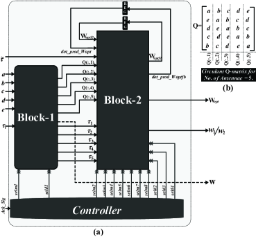
Figure 4: (a) Proposed system-level hardware-architecture of OEB for $N{=}5$ number of antennae (b) $\mathbf{Q}$ $\in$ $\mathbb{C}^{5{\times}5}$ circulant matrix containing 16-bit complex elements.

Subsequently, Block-2 of the proposed OEB has been designed to perform the operations of steps 8$-$21 in Algorithm 1. Here, Block-2 generates beamforming vectors $\mathbf{w}_{1}$ and $\mathbf{w}_{2}$ which are used for estimating $\tilde{\tau}_{1}$ and $\tilde{\tau}_{2}$ values, by another block that is excluded in Fig. 4 (a). These values are fed as $\tilde{\tau}$ to the proposed OEB architecture, as shown in Fig. 4 (a). It also shows that Block-2 has feedback information which is iteratively processed to generate the optimal beamforming vector $\mathbf{w}_{opt}$. Eventually, the controller has been designed to feed various control signals to both Block-1 and Block-2 modules of the OEB architecture. These control signals enable OEB to set the systematic flow of information in every iteration of calculating the optimal beamforming vector.

V-A Micro-architectures of Block-1 & Block-2

V-A1 Block-1

A detailed explanation of the hardware micro-architectures of OEB sub-modules is presented here. Firstly, the design of Block-1 micro-architecture that comprises register banks (RBs) and steering logics is presented in Fig. 5. It is fed (in single clock cycle) with five complex elements of $\mathbf{Q}$ matrix: a, b, c, d, and e where each of them is 16-bit represented fixed-point value. They are the first row elements of $\mathbf{Q}$ matrix, referring to Fig. 4 (b), and they are buffered in RB-1 of Block-1. Subsequently, RB-1 outputs are tapped and concatenated to generate five column vectors $-$$\mathbf{Q}$(:, 1) to $\mathbf{Q}$(:, 5)$-$ of 80 bit each which are stored in RB-2, as shown in Fig. 5. Further, these values from RB-2 are tapped as parallel outputs that will be later fed to Block-2. On the other hand, RB-2 outputs are also routed via multiplexer MUX1 and are transmitted as $\mathbf{w}$ vector for the computation of $\tau_{i}$ $\forall$ i = {1, 2, 3, 4, 5} values, as shown in Fig. 5. It also shows that the computed $\tau_{i}$ real-values (each of 8 bit) are sequentially fed to Block-1 architecture where they are routed to RB-3 via de-multiplexer DeMUX1. Eventually, these five parallel $\tau_{i}$ values are also projected as outputs of Block-1 design.

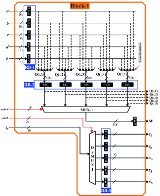
Figure 5: Proposed micro-architecture of the Block-1 submodule of OEB.

V-A2 Block-2

The proposed micro-architecture of Block-2 shown in Fig. 6 has been designed to perform the operations of steps 8$-$21 in Algorithm 1. To begin with, sub-module Block-2a executes steps 8$-$14 of Algorithm 1, as shown in Fig. 6. Here, MUX3 and MUX4 of Block-2a are responsible for assigning the input $\tau_{i}$ values (released from Block-1) to $\alpha_{1}$ and $\alpha_{2}$, respectively, corresponding to step 8 of Algorithm 1. Similarly, MUX2 and MUX5 are used for routing $\mathbf{Q}$(:, 1) to $\mathbf{Q}$(:, 5) input vectors into the datapath, as shown in Fig. 6. Subsequently, outputs of these multiplexers in Block-2a are processed by multipliers, adders, dividers, square-root computation unit, and MUX6, to generate $\kappa_{1}$, $\kappa_{2}$, and beamforming vectors ($\mathbf{w}_{1}$ and $\mathbf{w}_{2}$) that completes the operations till step 14 in Algorithm 1. These $\mathbf{w}_{1}$ and $\mathbf{w}_{2}$ vectors are transmitted for computing the $\tilde{\tau}_{1}$ and $\tilde{\tau}_{2}$ values, respectively. They are fed as $\tilde{\tau}$ input to Block-2a where the de-multiplexer DeMUX2 routes and buffers such sequentially generated values as $\tilde{\tau}_{1}$ and $\tilde{\tau}_{2}$, as shown in Fig. 6. It further shows that such $\tilde{\tau}$ and $\kappa$ values are arithmetically processed to compute $\gamma_{R}$ and $\gamma_{I}$ entities of step 15 in Algorithm 1. These $\gamma$ values are passed through 2’s complement units (2CUs) to realize ${-}\gamma_{R}$ and ${-}\gamma_{I}$ which are further divided and routed to coordinate rotations digital-computer (CORDIC) unit [37] via multiplexer MUX7, referring Fig. 6. Such MUX7 sequentially provides $\left(-\gamma_{I}/\gamma_{R}\right)$ and $\left(\gamma_{I}/-\gamma_{R}\right)$ values to the CORDIC unit that computes $\theta_{1}$ and $\theta_{2}$ values in resource shared manner. Subsequently, outputs of the CORDIC unit are de-multiplexed (by DeMUX3) to buffer $\theta_{1}$ and $\theta_{2}$ values that realizes step 16 of Algorithm 1.

Another set of CORDIC unit with multiplexer MUX8 has been used for computing sin($\theta_{1}$), sin($\theta_{2}$), cos($\theta_{1}$), and cos($\theta_{2}$), as shown in Fig. 6. These transcendental values are concatenated to realize $e^{(j{\cdot}\theta_{1})}$ and $e^{(j{\cdot}\theta_{2})}$ which are used for computing the $\mathbf{w}_{opt}$ values of steps 18 and 20 in Algorithm 1, and they are fed to multiplexer MUX10. In parallel, $\gamma_{R}{\cdot}$cos($\theta_{1}$)$-$$\gamma_{I}{\cdot}$sin($\theta_{1}$) value has been generated and its MSB is used as select line of MUX10 whose output (denoted as $\mathbf{w}_{optf1}$) is the compared value between $\mathbf{w}_{opt}$ values of steps 17 to 21 in Algorithm 1. Similarly, ${dot}\_{prod}\_{\mathbf{w}_{opt}}$ values of steps 18 and 20 in Algorithm 1 are computed and compared via multiplexer MUX9 whose output is denoted as ${dot}\_{prod}\_{\mathbf{w}_{optfb}}$ in Fig. 6. It shows that the aforementioned outputs from MUX9 and MUX10 are buffered and fed back to MUX3 and MUX2, respectively, in order to run multiple iterations between steps 7 to 22 in Algorithm 1.

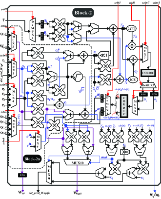
Figure 6: Proposed micro-architecture of the Block-2 submodule of OEB.

V-A3 Controller

Controller of the proposed OEB generates various select-line values as control signals for multiplexers (i.e. selm1$-$selm8) and de-multiplexers (i.e. seld1$-$seld4) to operate multiple iterations and direct the data for valid operation, as shown in Fig. 4. As presented in Algorithm 1, steps 2$-$3 and steps 11$-$14 operations wait for $\tau$ and $\tilde{\tau}$ values before transmitting the new $\mathbf{w}$ vector. Thereby, ${Ack}\_{Sig}$ has been used as a handshake/acknowledgement signal between such modules and the proposed OEB architecture. This ${Ack}\_{Sig}$ is fed to the controller of OEB that generates required control signals for Block-1 and Block-2 submodules. After all the iterations are executed, the optimal beamforming vector $\mathbf{w}_{opt}$ is eventually tapped from MUX2 as an output of the proposed OEB architecture, as shown in Fig. 6 and 4.

V-B FPGA Implementation and ASIC Design Results

The proposed OEB architecture for finding the optimal beamforming vector has been implemented on a field-programmable gate-array (FPGA) platform. Static timing analysis of this design indicates that our OEB prototype can operate with the maximum clock frequency of 44.25 MHz and its critical path delay is 22.6 ns. Hardware utilization of the OEB architecture when implemented on Nexys4 DDR (xc7a100tcsg324-1) FPGA-board has been comprehensively presented in Table I. It also shows the segregated hardware-consumption details of Block-1, Block-2, and controller micro-architectures of OEB. Here, Block-2 consumes the maximum FPGA resources of 3661 look-up tables (LUTs), 897 flip-flops (FFs), and 24 digital signal processor (DSP) cores.

Furthermore, the suggested OEB architecture has been ASIC synthesized and post-layout simulated in a 90 nm-CMOS technology node. Industry-standard electronics design automation (EDA) tools are used to perform frontend and physical design processes where the former includes functional validation, gate-level synthesis, static timing analysis, and post-synthesis simulations. On the other hand, the physical design process includes floorplan, standard-cell placement, power planning, signal routing, clock tree synthesis, timing verification, and finally the post-layout simulation. Outcomes of such ASIC design processes are presented in Table II where the design parameters of Block-1, Block-2, and Controller modules of the proposed OEB are separately listed. In addition, Table II also shows that an overall OEB design occupies an area of 0.21 mm² and it is capable of operating with a maximum clock frequency of 120 MHz. At the supply voltage of 1.2 V, it consumes dynamic power of 44385.7 pW while operating at 120 MHz of clock frequency and static power consumption of 816.61 pW, as shown in Table II.

TABLE I: Hardware Utilization of the Proposed OEB Architecture Implemented on Nexys4-DDR (xc7a100tcsg324-1) FPGA-Board

	Block-1	Block-2	Controller	OEB
Number of LUTs	169	3661	150	3980
Number of FFs	371	897	43	1311
Number of F7 MUXes	80	0	0	80
Number of DSP Cores	0	24	0	24

TABLE II: ASIC Synthesis and Post-Layout Simulation Results of Suggested OEB Architecture in UMC 90 nm-CMOS Process

	Block-1	Block-2	Controller	OEB
Technology (nm)	90	90	90	90
Supply Voltage (V)	1.2	1.2	1.2	1.2
Silicon Area (mm2)	0.012	0.173	0.00033	0.21
Standard Cell Count	946	17208	39	18193
Crit. Path Delay (ps)	1744	8784	1411	8784
Max. Clk Freq. (GHz)	0.57	0.114	0.71	0.12
Dynamic Power (pW)	2285.2	42060.5	39.99	44385.7
Leakage Power (pW)	46.6	768.7	1.311	816.61
Bit Quantization (bits)	16	16	16	16

VI Numerical results

In this section, through numerical computation we evaluate the performance of the proposed algorithm by varying relevant system parameters. As the article focuses on improving the energy delivery, as elaborated in section III, we consider only those parameters that are relevant to energy transmission and harvesting. Table III summarises the parameters considered in the evaluation of the proposed algorithm, where the values of some parameters are taken from [8, 13, 34].

TABLE III: Table of the parameters used in numerical computation.

Parameter	Value(s)/range
Transmit power, $P_{t}$	$3-10$ Watts
No. of antennas at the Tx, $N$	$5,10$
Antenna gain, $G$	$1$
Distance between Energy Tx & Rx, $L$	$3-10$ meters
Pathloss exponent, $\beta$	$3$
Rician factor, $K_{f}$	$2,10$
Resistance (Energy storage), $R$	$100$ $\Omega$
Capacitance (Energy storage), $C$	$1$mF
Initial charge level, $q_{0}$	$1.5$ mC
Maximum charge level, $q_{m}$	$3$ mC
Time limit, $t_{lim}$	$100$ seconds

As the maximum distance between the energy transmitter and the energy receiver is $10$ meters (cf. Table III), we assume the channel is characterised by a dominant line-of-sight (LoS) component. Similar to [13], we consider Rician fading channel to model the channel between the two devices. Specifically, we consider the following three channels for the performance evaluation (i) Fading channel with Rician factor ($K_{f}$) = 2, (ii) Fading channel with $K_{f}=10$ and (iii) Deterministic channel (corresponding to $K_{f}\to\infty$). We also incorporate the path-loss with the help of the path-loss exponent $\beta$. It should be noted that the plots presented in this section are generated by averaging over 1000 realisations of fading channels mentioned previously. Furthermore, we assume the following piece-wise linear energy harvesting efficiency function for calculating the harvested power at the receiver.

$$\eta=\begin{cases}0,&P_{r}<p_{th,0}\\ \eta_{0}\frac{(Pr-p_{th,0})}{p_{th,1}-p_{th,0}},&p_{th,0}\leq P<p_{th,1}\\ \eta_{0}+(\eta_{1}-\eta_{0})\frac{(P_{r}-p_{th,1})}{p_{th,2}-p_{th,1}},&p_{th,1}\leq P_{r}<p_{th,2}\\ \eta_{1}+(\eta_{2}-\eta_{1})\frac{(P_{r}-p_{th,2})}{p_{th,3}-p_{th,2}},&p_{th,2}\leq P_{r}\leq p_{th,3}\\ \eta_{2},&P_{r}>p_{th,3},\end{cases}$$ (17)

with $\eta_{0}=0.4$, $\eta_{1}=0.6$, $\eta_{2}=0.65$, $p_{th,0}=10^{-6}$ , $p_{th,1}=10^{-5}$, $p_{th,2}=10^{-4}$ and $p_{th,3}=10^{-3}$.

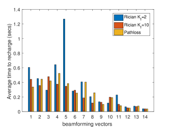
Figure 7: Average time-to-recharge and average harvested power due to different beamforming vectors during the feedback acquisition and processing phase for considered channels. The transmit power is set to $10$ Watts and the distance between the energy transmitter and harvester is $5$ meters.

In Fig. 7, we depict the average time-to-recharge and average harvested power due to beamforming vectors employed by the proposed algorithm during the FAP phase. As the energy transmitter considered for this figure has $5$ antennas, the FAP phase spans time-to-recharge duration of $13$ beamforming vectors indexed by ordinal numbers. The first five set of bars in Figs. 7 and 7 correspond to five beamforming vectors obtained from columns of $\mathbf{Q}$. The following eight set of bars correspond to the intermediate beamforming vectors obtained through linear combinations of columns of $\mathbf{Q}$. The last set of bars correspond to the optimal beamforming vector obtained at the end of the FAP phase. It is evident that the sixth beamforming vector onward the harvested power increases and consequently, the time-to-recharge decreases as the algorithm produces vectors that approach the optimal beamforming vector. It should be noted that time-to-recharge values were capped at $t_{lim}$ mentioned in Table III.

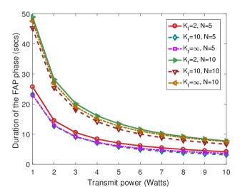
Figure 8: Average duration of the FAP phase with respect to the transmit power for different channels types and $5,10$ antennas at the transmitter. The distance between the energy transmitter and harvester is $5$ meters.

Fig. 8 plots the duration of the FAP phase with respect to the transmit power at the energy transmitter for $5$ and $10$ antenna systems when the receiver is $5$ meters away. The duration of the FAP phase of the latter is almost double of the former and can be explained by counting the number of slots in the respective FAP phases (i.e., $13$ and $28$). While a longer FAP phase might seem disadvantageous, one must not forget that a proportionately larger number of recharging cycle (and the subsequent information transmission) is completed during that phase. The duration of the FAP phase for both $5$ and $10$ antenna transmitters decreases with the transmit power, which is intuitive. Fig. 9, on the other hand, portrays the variation of the harvested energy with respect to the transmit power. The $10$-antenna transmitter is able to deliver approx $3\times$ energy compared with the $5$-antenna transmitter due to $2\times$ number antennas and $\approx 2\times$ slots in the FAP phase. Similar to the Fig. 8, the increase in the harvested energy with transmit power is apparent.

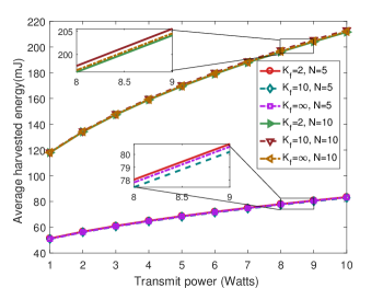
Figure 9: Average harvested energy during the FAP phase vs. transmit power for different channel types and $5,10$ antennas at the transmitter. The distance between the energy transmitter and harvester is $5$ meters.

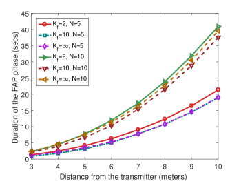
Figure 10: Average duration of the FAP phase with respect to the distance between the energy transmitter and harvester for different channel types and $5,10$ antennas at the transmitter. The transmit power is set to $10$ W.

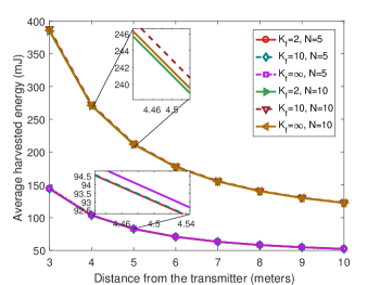
Figure 11: Average harvested energy during the FAP phase with respect to the distance between the energy transmitter and harvester for different channel types and $5,10$ antennas at the transmitter. The transmit power is set to $10$ W.

In Fig. 10 and 11, we plot the duration of the FAP phase and the energy harvested in that phase, respectively, with respect to the distance of the receiver from the transmitter while fixing the transmit power to $10$ Watts. As the distance increases, the received power decreases and the subsequently the duration of the FAP phase increases for both $5$ and $10$ antenna transmitters. In both plots, the values plotted in $y$-axis varies in proportion to the number of antennas, similar to that of Fig. 8 and 9.

VII Conclusion

In this article, we presented a scheme to find the optimal beamforming vector for the energy beamforming at a transmitter from indirect feedback collected from a energy receiver. The proposed scheme exploits the dynamics of the harvest-then-transmit protocol and the inherent latency of the charging process to extract a temporal feedback about the beamforming vector used by the transmitter. As the receiver’s energy is preserved in the proposed scheme, a higher throughput or reduced latency in information transmission, and energy saving at the transmitter are guaranteed, leading to an improved WPT system. The presented scheme is supplemented by an algorithm and its hardware architecture for facilitating its adoption in various real-world WPT implementations. Hardware utilisation details, ASIC synthesis and post-layout simulation results were presented to substantiate the proposed architecture. Lastly, through numerical results we demonstrated the performance of the proposed scheme with respect to various system parameters.

References

- [1] H. Ju and R. Zhang, “Throughput Maximization in Wireless Powered Communication Networks,” IEEE Transactions on Wireless Communications, vol. 13, no. 1, pp. 418–428, January 2014.
- [2] J. Xu and R. Zhang, “Energy beamforming with one-bit feedback,” IEEE Transactions on Signal Processing, vol. 62, no. 20, pp. 5370–5381, 2014.
- [3] X. Chen, C. Yuen, and Z. Zhang, “Wireless energy and information transfer tradeoff for limited-feedback multiantenna systems with energy beamforming,” IEEE Transactions on Vehicular Technology, vol. 63, no. 1, pp. 407–412, 2013.
- [4] R. Zhang and C. K. Ho, “MIMO Broadcasting for Simultaneous Wireless Information and Power Transfer,” IEEE Transactions on Wireless Communications, vol. 12, no. 5, pp. 1989–2001, May 2013.
- [5] H. Lee, S.-R. Lee, K.-J. Lee, H.-B. Kong, and I. Lee, “Optimal beamforming designs for wireless information and power transfer in miso interference channels,” IEEE Transactions on Wireless Communications, vol. 14, no. 9, pp. 4810–4821, 2015.
- [6] B. Clerckx, R. Zhang, R. Schober, D. W. K. Ng, D. I. Kim, and H. V. Poor, “Fundamentals of wireless information and power transfer: From rf energy harvester models to signal and system designs,” IEEE Journal on Selected Areas in Communications, vol. 37, no. 1, pp. 4–33, 2019.
- [7] E. Boshkovska, D. W. K. Ng, N. Zlatanov, A. Koelpin, and R. Schober, “Robust resource allocation for mimo wireless powered communication networks based on a non-linear eh model,” IEEE Transactions on Communications, vol. 65, no. 5, pp. 1984–1999, 2017.
- [8] L. Liu, R. Zhang, and K. C. Chua, “Multi-antenna wireless powered communication with energy beamforming,” IEEE Transactions on Communications, vol. 62, no. 12, pp. 4349–4361, Dec 2014.
- [9] J. Xu, L. Liu, and R. Zhang, “Multiuser miso beamforming for simultaneous wireless information and power transfer,” IEEE Transactions on Signal Processing, vol. 62, no. 18, pp. 4798–4810, 2014.
- [10] H. Son and B. Clerckx, “Joint beamforming design for multi-user wireless information and power transfer,” IEEE Transactions on Wireless Communications, vol. 13, no. 11, pp. 6397–6409, 2014.
- [11] Q. Shi, L. Liu, W. Xu, and R. Zhang, “Joint transmit beamforming and receive power splitting for miso swipt systems,” IEEE Transactions on Wireless Communications, vol. 13, no. 6, pp. 3269–3280, 2014.
- [12] S. Timotheou, I. Krikidis, G. Zheng, and B. Ottersten, “Beamforming for miso interference channels with qos and rf energy transfer,” IEEE Transactions on Wireless Communications, vol. 13, no. 5, pp. 2646–2658, 2014.
- [13] Y. Zeng and R. Zhang, “Optimized training design for wireless energy transfer,” IEEE Transactions on Communications, vol. 63, no. 2, pp. 536–550, 2014.
- [14] ——, “Optimized training for net energy maximization in multi-antenna wireless energy transfer over frequency-selective channel,” IEEE Transactions on Communications, vol. 63, no. 6, pp. 2360–2373, 2015.
- [15] G. Yang, C. K. Ho, and Y. L. Guan, “Dynamic resource allocation for multiple-antenna wireless power transfer,” IEEE Transactions on Signal Processing, vol. 62, no. 14, pp. 3565–3577, 2014.
- [16] S. Lee and R. Zhang, “Distributed wireless power transfer with energy feedback,” IEEE Transactions on Signal Processing, vol. 65, no. 7, pp. 1685–1699, 2016.
- [17] K. W. Choi, D. I. Kim, and M. Y. Chung, “Received power-based channel estimation for energy beamforming in multiple-antenna rf energy transfer system,” IEEE Transactions on Signal Processing, vol. 65, no. 6, pp. 1461–1476, 2016.
- [18] K. W. Choi, L. Ginting, P. A. Rosyady, A. A. Aziz, and D. I. Kim, “Wireless-powered sensor networks: How to realize,” IEEE Transactions on Wireless Communications, vol. 16, no. 1, pp. 221–234, 2016.
- [19] J. Xu and R. Zhang, “A general design framework for mimo wireless energy transfer with limited feedback,” IEEE Transactions on Signal Processing, vol. 64, no. 10, pp. 2475–2488, 2016.
- [20] S. Abeywickrama, T. Samarasinghe, C. K. Ho, and C. Yuen, “Wireless energy beamforming using received signal strength indicator feedback,” IEEE Transactions on Signal Processing, vol. 66, no. 1, pp. 224–235, 2018.
- [21] R. Zhang, “On active learning and supervised transmission of spectrum sharing based cognitive radios by exploiting hidden primary radio feedback,” IEEE Transactions on Communications, vol. 58, no. 10, pp. 2960–2970, 2010.
- [22] Y. Noam and A. J. Goldsmith, “Blind null-space learning for mimo underlay cognitive radio with primary user interference adaptation,” IEEE Transactions on Wireless Communications, vol. 12, no. 4, pp. 1722–1734, 2013.
- [23] D. Mishra, S. De, and K. R. Chowdhury, “Charging time characterization for wireless rf energy transfer,” IEEE Transactions on Circuits and Systems II: Express Briefs, vol. 62, no. 4, pp. 362–366, 2015.
- [24] R. B. Chaurasiya and R. Shrestha, “Design and asic-implementation of hardware-efficient cooperative spectrum-sensor for data fusion based cognitive radio network,” IEEE Transactions on Consumer Electronics, vol. 68, no. 3, pp. 221–235, 2022.
- [25] A. Verma and R. Shrestha, “Low computational-complexity soms-algorithm and high-throughput decoder architecture for qc-ldpc codes,” IEEE Transactions on Vehicular Technology, 2022.
- [26] Y. Zhang and B. Clerckx, “Waveform design for wireless power transfer with power amplifier and energy harvester non-linearities,” arXiv preprint arXiv:2204.00957, 2022.
- [27] X. Lu, P. Wang, D. Niyato, D. I. Kim, and Z. Han, “Wireless Networks With RF Energy Harvesting: A Contemporary Survey,” IEEE Communications Surveys Tutorials, vol. 17, no. 2, pp. 757–789, Secondquarter 2015.
- [28] “Powercast P2110B.” [Online]. Available: https://www.powercastco.com/documentation/
- [29] Y. Huang and B. Clerckx, “Large-scale multiantenna multisine wireless power transfer,” IEEE Transactions on Signal Processing, vol. 65, no. 21, pp. 5812–5827, 2017.
- [30] J. D. Griffin and G. D. Durgin, “Complete link budgets for backscatter-radio and rfid systems,” IEEE Antennas and Propagation Magazine, vol. 51, no. 2, pp. 11–25, 2009.
- [31] C. R. Valenta and G. D. Durgin, “Harvesting wireless power: Survey of energy-harvester conversion efficiency in far-field, wireless power transfer systems,” IEEE Microwave Magazine, vol. 15, no. 4, pp. 108–120, 2014.
- [32] D. Mishra and S. De, “Utility maximization models for two-hop energy relaying in practical rf harvesting networks,” in 2017 IEEE International Conference on Communications Workshops (ICC Workshops). IEEE, 2017, pp. 41–46.
- [33] P. N. Alevizos and A. Bletsas, “Sensitive and nonlinear far-field rf energy harvesting in wireless communications,” IEEE Transactions on Wireless Communications, vol. 17, no. 6, pp. 3670–3685, 2018.
- [34] S. Sarma and K. Ishibashi, “Time-to-recharge analysis for energy-relay-assisted energy harvesting,” IEEE Access, vol. 7, pp. 139 924–139 937, 2019.
- [35] Y. Chen, K. T. Sabnis, and R. A. Abd-Alhameed, “New formula for conversion efficiency of rf eh and its wireless applications,” IEEE Transactions on Vehicular Technology, vol. 65, no. 11, pp. 9410–9414, 2016.
- [36] S. Abeywickrama, R. Zhang, and C. Yuen, “Refined nonlinear rectenna modeling and optimal waveform design for multi-user multi-antenna wireless power transfer,” IEEE Journal of Selected Topics in Signal Processing, vol. 15, no. 5, pp. 1198–1210, 2021.
- [37] R. Andraka, “A survey of cordic algorithms for fpga based computers,” in Proceedings of the 1998 ACM/SIGDA sixth international symposium on Field programmable gate arrays, 1998, pp. 191–200.