Bilinearization of the Fokas-Lenells equation Conservation laws and soliton interactions

Abstract

In this paper, we propose the bilinearization of the Fokas-Lenells equation (FLE) with a vanishing boundary condition. In the proposed bilinearization we make use of an auxiliary function to convert the trilinear equations into a set of bilinear equations. We obtain bright $1$-soliton, $2$- soliton solutions and present the scheme for obtaining $N$ soliton solution. In the soliton solution the presence of an additional parameter allows tuning the position of soliton. We find that the proposed scheme of bilinearization using auxiliary function, considerably simplifies the procedure yet generates a more general solution than the one reported earlier. We show that the obtained soliton solution reduces to an algebraic soliton in the limit of infinite width. Further we show explicitly that the soliton interactions are elastic through asymptotic analysis, that is the amplitude of each soliton remains same before and after interaction. The mark of interaction is left behind only in the phase of each soliton. Secondly, we propose a generalised Lax pair for the FLE and obtain the conserved quantities by solving Riccati equation. We believe that the present investigation would be useful to study the applications of FLE in nonlinear optics and other branches of physics.

1 Introduction

Fokas-Lenells equation (FLE) [1, 2] is one of the four categories of integrable equations which describes the propagation of ultrashort pulses in nonlinear medium. The other three are namely, nonlinear Schrödinger equation (NLSE) [3, 4], derivative NLSE (DNLSE) [5], higher order NLSE (HNLSE) [6, 7]. All four equations play significant role in the study of localised waves in nonlinear optical medium [16, 17, 4, 18]. A common property in all these physical systems is the appearance of solitons, which arise as a result of a balance between the nonlinear and dispersive terms of the wave equations [16]. In comparison to NLSE, the significance of FLE is due to the presence of a spatio-temporal dispersion term in addition to the group velocity dispersion term. While the study on three other equations is done extensively, the study on FLE is relatively sparse. A few notable contributions on FLE are interaction between different localised waves [8], solitary wave and elliptical solutions of FLE in presence of perturbation and modulation instability [9], combined optical solitary waves of FLE [22], dynamical behaviour of soliton solutions of FLE [10], inverse transform of FLE with nonzero boundary condition [11], optical soliton perturbation with FLE by different methods [12, 23], derivation of dimensionless FLE with perturbation term [13].

The dimensionless form of FLE [1, 2] :

$$iU_{t}+a_{1}U_{xx}+b|U|^{2}U+a_{2}(U_{xt}+ib|U|^{2}U_{x})=0$$ (1)

where $U$ is the envelope function of an optical field. It can describe the ultrashort pulse propagation of an optical field in a medium where the beam is allowed to diffract along one of the two, namely longitudinal and transverse directions. An important fact about the FLE is that a gauge transformation of FLE belongs to the hierarchy of integrable DNLSE [14, 15]. Localised solutions of FLE are obtained in different forms, namely solitary waves [2], ’W’-shaped and other solitons [20], soliton solution using inverse scattering transform [11], using Darboux transformation [25], using some other different methods [21]. N-soliton solution in $\tau$- function is obtained in [14].

In this manuscript our objective is to propose an alternate simplified and systematic scheme, namely bilinearization by introducing an auxiliary function and obtain a generalized expression for multi-soliton solutions.

Secondly, a limited class of soliton bearing equations exhibits an interesting property and belongs to the exclusive club of integrable systems [19]. The most prominent definition of integrability is the integrability in the Liouville sense, that is the existence of a set of infinite functionally independent conserved quantities, which are in involution [19]. Importantly, the Poisson brackets of these conserved quantities with one another vanishes.

Extraction of the conserved quantities for the FLE and establishing the integrability of the hierarchy in the Liouville sense remained unexplored till date. Thus our second objective is to obtain the same by solving the Riccati equation for the $2\times 2$ dimensional Lax operator and consequently to obtain the whole hierarchy of conserved charges in a systematic way.

The structure of the manuscript is the following. In the following section we shall consider the gauge transformed FLE. The bilinearization of FLE and one soliton solutions including algebraic soliton are described in this section. Two Soliton interaction using asymptotic analysis will be discussed in the third section. Fourth section will cover the conserved quantities which are obtained by using Lax pair and solving the Riccati equation. Fifth section will be the concluding one.

2 Bilinearization of FLE with vanishing background

The gauge transformation,

$$U=\sqrt{\frac{m}{|b|}}ne^{i(nx+2mnt)}u$$ (2)

followed by transformation of variables,

$$\xi=x+mt;\quad\tau=-mn^{2}t,$$ (3)

where $n=\frac{1}{a_{2}}$ and $m=-\frac{a_{1}}{a_{2}}$. converts eq. 1 into

$$u_{\xi\tau}=u-2i\sigma|u|^{2}u_{\xi}$$ (4)

Under the vanishing background condition $|u|\rightarrow 0$ as $|\xi|\rightarrow\pm\infty$ we expect a bright soliton solution by applying the bilinearization method.

To write eq. 4 in the bilinear form let us assume

$$q=\frac{g}{f}$$ (5)

where $g$ and $f$ are two complex functions of ($\xi,\ \tau$). Using eq. 5 and eq. 4 we obtain a nonlinear equation in terms of newly introduced fields,

$$\frac{1}{f^{2}}(D_{\xi}D_{\tau}-1)g.f-\frac{g}{f^{3}}D_{\xi}D_{\tau}(f.f)+\frac{2i|g|^{2}}{f^{3}f^{*}}D_{\xi}(g.f)+\frac{s|g|^{2}}{f^{3}}-\frac{s|g|^{2}f^{*}}{f^{3}f^{*}}=0$$ (6)

where $D_{\xi}$, $D_{\tau}$ are the Hirota derivatives[6, 28], which are defined as

$$D_{\xi}^{m}D_{\tau}^{n}g(\xi,\tau).f(\xi,\tau)=(\frac{\partial}{\partial\xi}-\frac{\partial}{\partial\xi^{\prime}})^{m}(\frac{\partial}{\partial\tau}-\frac{\partial}{\partial\tau^{\prime}})^{n}g(\xi,\tau).f(\xi^{\prime},\tau^{\prime})\Bigg{|}_{(\xi=\xi^{\prime})(\tau=\tau^{\prime})}$$ (7)

Notice that the last two terms in eq. 6 contain an auxiliary function $s$, which is introduced so that eq. 6 can be cast into following bilinear equations in terms of $g$, $f$ and $s$.

$$(D_{\xi}D_{\tau}-1)g.f =0$$ (8)

$$D_{\xi}D_{\tau}(f.f) =sg^{*}$$ (9)

$$2iD_{\xi}(g.f) =sf^{*}$$ (10)

To obtain the soliton solution, $g$ and $f$ are expanded with respect to an arbitrary parameter $\epsilon$ as follows:

$$g =\epsilon g_{1}+\epsilon^{3}g_{3}+.....$$ (11)

$$f =f_{0}+\epsilon^{2}f_{2}+\epsilon^{4}f_{4}+.....$$ (12)

The auxiliary function is expanded as

$$s=\epsilon s_{1}+\epsilon^{3}s_{3}+.....$$ (13)

2.1 Bright soliton

The one soliton solution (1-SS) of eq. 4 is obtained by using eqs. 5, 11 - 13, subsequently dropping terms of order greater than or equal to $\epsilon^{3}$ in $g$ and $f$ and $s$. That is,

$$q=\frac{\epsilon g_{1}}{f_{0}+\epsilon^{2}f_{2}}\Big{|}_{\epsilon=1}$$ (14)

Let us consider

$$g_{1} =\alpha e^{\theta(\xi,\tau)}$$ (15)

$$f_{0} =\beta;\quad f_{2}=\beta_{2}e^{\theta(\xi,\tau)+\theta^{*}(\xi,\tau)}$$ (16)

$$s =ce^{\theta(\xi,\tau)}$$ (17)

substituting eqs. 14 -17 in eqs. 8- 10 we obtain the 1-SS, where the parameters are

$$\theta =p\ \xi+\frac{1}{p}\tau+\theta_{0}$$ (18)

$$\beta_{2} =i\frac{|\alpha|^{2}|p|^{2}p}{\beta^{*}(p+p^{*})^{2}};\quad\quad c=\frac{2i\beta\alpha p}{\beta^{*}}$$ (19)

$\alpha$, $\beta$ and $p$ are arbitrary complex constants. $\theta_{0}$ is also a complex constant representing the initial phase.

Notice that due to the introduction of an auxiliary function the bilinearization process becomes considerably straightforward as compared to the earlier reported methods [11, 14]. The additional parameter $\beta$ introduced in the solution is responsible for the shift in the central position of the soliton. Other than that $\beta$ does not interfere with other soliton properties. Figure 1 shows the shift in the position of the soliton with change in $\beta$. Notice that for $\alpha=-(p+p^{*})$ and $\beta=-i|p|^{2}$ eq. 14 reduces to the soliton solution obtained in [14].

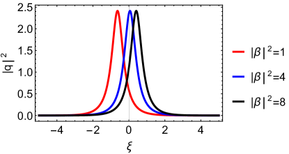
Figure 1: Shift in the soliton position with respect to $\beta$.

We may further identify the following physical quantities associated with the soliton wave, namely wave number, $k=\frac{-i}{2}(p-p^{*})$, the frequency shift, $\Omega(k)=\frac{\frac{i}{2}(p-p^{*})}{|p|^{2}}$, the soliton velocity, $v=-\frac{d\Omega}{dk}=\frac{1}{|p|^{2}}$ and the width inverse, $a=\frac{1}{2}(p+p^{*})$. Further we may write the amplitude in terms of velocity as $A=\sqrt{v}\sqrt{2(\frac{1}{\sqrt{v}}+k)}$. Notice that the amplitude vs velocity is not linear as in the case of conventional NLSE soliton [3] but has an interesting relationship where the amplitude of soliton is a function of two of the following parameters, ’$k$, $v$ and $a$’. The same is illustrated in figure 2 (a, b).

Figure 2 shows amplitude ($A$) vs velocity ($v$) graph for (a) $k=0,1,2$ and (b) $k=-1,-2,-3$. It shows that for positive values of $k$, the amplitude increases monotonically with the increase in $v$. For negative values of $k$, the relation is not monotonic. The amplitude increases initially and reaches a maximum value at $v=\frac{1}{4b^{2}}$ and then decreases.

Figure 3 shows amplitude (A) vs width inverse ($a$) graphs for (a) $k=0,1,2$ and (b) $k=-1,-2,-3$. Notice that for positive values of $k$, the amplitude decreases monotonically with the increase in $a$. For negative values of $k$, the relation is however not monotonic. The amplitude increases initially and reaches a maximum value at $a=-\sqrt{3}b$ and then decreases.

The above mentioned properties are quite unique and in contrast to that of the conventional NLSE soliton.

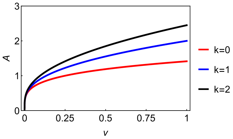
(a)

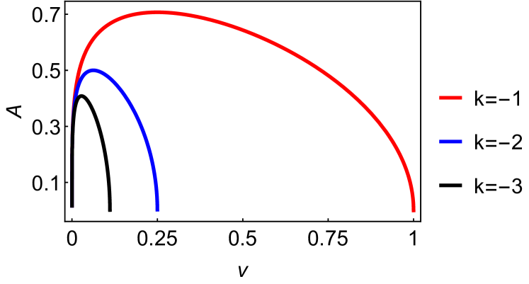
(b)

Figure 2: (a) Variation of amplitude with velocity for positive values of wave vector (k)  (b) Variation of amplitude with velocity for negative values of wave vector

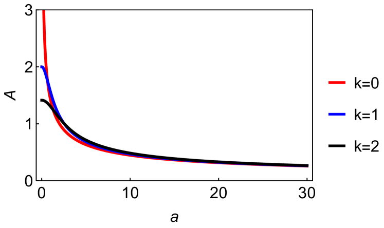
(a)

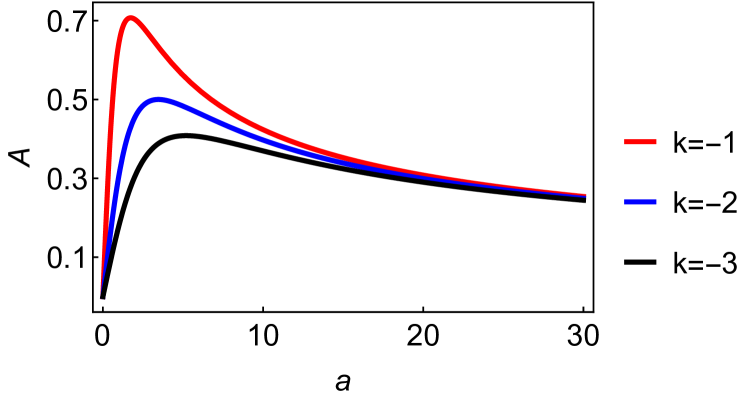
(b)

Figure 3: (a) Variation of amplitude with width inverse for positive values of wave vector (k)  (b) Variation of amplitude with width inverse for negative values of wave vector

2.2 Algebraic Soliton

One unique feature of FLE soliton is that in the limit of infinite width ($a\rightarrow 0$) FLE soliton does not vanish but the amplitude reduces to a finite value. To show this let us consider $\beta={p^{*}}^{2}$, $\alpha=(p+p^{*})$ and the phase $\theta_{0}=ax_{0}+2\delta$ where $e^{2\delta}=k$. The 1-SS from eq. 14 then reduces to the form,

$$q=\frac{-e^{i\chi(\xi,\tau)}}{(\xi+v\tau+x_{0})-ik}$$ (20)

where $\chi(\xi,\tau)=k\ \xi-\frac{\tau}{k}+\chi_{0}$,   $\chi_{0}$ is a constant phase of the oscillating function.
Eq. 20 is nothing but the expression of an algebraic soliton, where the envelope function disappears giving rise to an algebraic form. However the soliton properties are still maintained. In the limit $a\to 0$,   the amplitude of the soliton reduces to a non-zero finite value and is proportional to $\sqrt{v}$. This is unlike conventional NLSE soliton, where the amplitude tends to zero in the limit of infinite width ($a\rightarrow 0$). Further notice that in the process of algebraic reduction two of the free parameters, $\alpha$ and $\beta$ have been constrained and thus leaving behind only one free parameter, namely the wave vector $k$. Figure 4 shows (a) the density plot of a soliton with $a=1$, $k=2$,  $\alpha=1+2i$,  $\beta=1+i$ (b) 2D plot of an algebraic soliton with $k=2$, in comparison to the soliton (a).

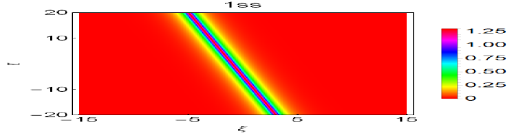
(a)

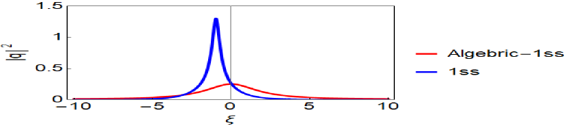
(b)

Figure 4: Density plot of (a) one soliton in component $|q|$ with $a=1$, $k=2$, $\alpha=1+2i$ and $\beta=1+i$.  (b) 2D plot of a normal soliton given in (a) and an algebraic soliton with $\ k=2$.

3 Two Soliton

The two soliton solution ($2$-SS) of FLE eq. 4 is obtained from eq. 5 by dropping terms of order greater than or equal to $\epsilon^{5}$ in $g$, $f$ and $s$ in eqs. 11-13.

$$q=\frac{\epsilon g_{1}+\epsilon^{3}g_{3}}{f_{0}+\epsilon^{2}f_{2}+\epsilon^{4}f_{4}}\Big{|}_{\epsilon=1}$$ (21)

Let us consider,

$$g_{1} =\alpha_{1}e^{\theta_{1}(\xi,\tau)}+\alpha_{2}e^{\theta_{2}(\xi,\tau)}$$ (22)

$$g_{3} =\alpha_{3}e^{\theta_{1}(\xi,\tau)+\theta^{*}_{1}(\xi,\tau)+\theta_{2}(\xi,\tau)}+\alpha_{4}e^{\theta_{1}(\xi,\tau)+\theta_{2}(\xi,\tau)+\theta^{*}_{2}(\xi,\tau)}$$ (23)

$$f_{0} =\beta;\quad\ f_{2}=\beta_{2}e^{\theta_{1}(\xi,\tau)+\theta^{*}_{1}(\xi,\tau)}+\beta_{3}e^{\theta_{2}(\xi,\tau)+\theta^{*}_{2}(\xi,\tau)}$$

$$+\beta_{4}e^{\theta_{1}(\xi,\tau)+\theta^{*}_{2}(\xi,\tau)}+\beta_{5}e^{\theta^{*}_{1}(\xi,\tau)+\theta_{2}(\xi,\tau)}$$ (24)

$$f_{4} =\beta_{6}e^{\theta_{1}(\xi,\tau)+\theta^{*}_{1}(\xi,\tau)+\theta_{2}(\xi,\tau)+\theta^{*}_{2}(\xi,\tau)}$$ (25)

$$s =c_{1}e^{\theta_{1}(\xi,\tau)}+c_{2}e^{\theta_{2}(\xi,\tau)}+c_{3}e^{\theta_{1}(\xi,\tau)+\theta^{*}_{1}(\xi,\tau)+\theta_{2}(\xi,\tau)}$$

$$+c_{4}e^{\theta_{1}(\xi,\tau)+\theta_{2}(\xi,\tau)+\theta^{*}_{2}(\xi,\tau)}$$ (26)

Substituting eqs. 21- 3 in eqs. 8 - 10 we obtain the following parameters,

$$\theta_{1} =p_{1}\ \xi+\frac{1}{p_{1}}\tau+\theta_{10};\quad\quad\theta_{2}=p_{2}\ \xi+\frac{1}{p_{2}}\tau+\theta_{20}$$

$$\alpha_{3} =\frac{i|\alpha_{1}|^{2}\alpha_{2}{p^{*}_{1}}^{3}(p_{1}-p_{2})^{2}}{|\beta|^{2}(p_{1}+p^{*}_{1})^{2}(p^{*}_{1}+p_{2})^{2}};\alpha_{4}=\frac{i|\alpha_{2}|^{2}\alpha_{1}{p^{*}_{2}}^{3}(p_{1}-p_{2})^{2}}{|\beta|^{2}(p_{2}+p^{*}_{2})^{2}(p_{1}+p^{*}_{2})^{2}}$$

$$\beta_{2} =\frac{i|\alpha_{1}|^{2}|p_{1}|^{2}p_{1}}{\beta^{*}(p_{1}+p^{*}_{1})^{2}};\quad\quad\quad\hskip 5.0pt\beta_{3}=\frac{i|\alpha_{2}|^{2}|p_{2}|^{2}p_{2}}{\beta^{*}(p^{*}_{2}+p_{2})^{2}}$$

$$\beta_{4} =\frac{i\alpha^{*}_{2}\alpha_{1}{p_{1}}^{2}p^{*}_{2}}{\beta^{*}(p_{1}+p^{*}_{2})^{2}};\quad\quad\quad\hskip 5.0pt\beta_{5}=\frac{i\alpha_{2}\alpha^{*}_{1}p_{2}^{2}p_{1}^{*}}{\beta^{*}(p_{2}+p^{*}_{1})^{2}}$$

$$\beta_{6} =\frac{-p_{1}p_{2}|p_{1}|^{2}|p_{2}|^{2}|\alpha_{1}|^{2}|\alpha_{2}|^{2}|(p_{1}-p_{2})|^{4}}{\beta^{*}|\beta|^{2}(p_{1}+p^{*}_{1})^{2}(p^{*}_{1}+p_{2})^{2}(p_{1}+p^{*}_{2})^{2}(p_{2}+p^{*}_{2})^{2}}$$

$\beta$, $\alpha_{1}$ ,$\alpha_{2}$ and $p_{1}$ ,$p_{2}$ are arbitrary complex constants.

To study the amplitudes and the phase shift of $2$-soliton we use asymptotic analysis.

3.1 Asymptotic analysis

When asymptotically apart from each other multi-solitons are essentially separated single solitons [28]. For asymptotic analysis let us consider two bright solitons $q_{1}$ and $q_{2}$ which interact as they move with a relative velocity.

Before interaction as $\tau\rightarrow-\infty$,

$$q_{1}=\frac{\alpha_{1}e^{p_{1}\xi+\frac{\tau}{p_{1}}}}{\beta+\beta_{2}e^{(p_{1}+p^{*}_{1})\xi+(\frac{1}{p_{1}}+\frac{1}{p^{*}_{1}})\tau}};$$ (27)

$$\theta_{1}(\xi,\ \tau)\to 0;\quad\theta_{2}(\xi,\ \tau)\to-\infty$$

$$q_{2}=\frac{\alpha_{3}e^{p_{2}\xi+\frac{\tau}{p_{2}}}}{\beta_{2}+\beta_{6}e^{(p_{2}+p^{*}_{2})\xi+(\frac{1}{p_{2}}+\frac{1}{p^{*}_{2}})\tau}};$$ (28)

$$\theta_{2}(\xi,\ \tau)\to 0;\quad\theta_{1}(\xi,\ \tau)\to\infty$$

Consequently,

$$|q_{1}|^{2}=\frac{2a^{2}_{1}}{(a^{2}_{1}+b^{2}_{1})^{3/2}}\times\frac{1}{cosh[2(\theta_{1}+ln\ \delta_{1})]-\frac{b_{1}}{\sqrt{a^{2}_{1}+b^{2}_{1}}}}$$ (29)

$$|q_{2}|^{2}=\frac{2a^{2}_{2}}{(a^{2}_{2}+b^{2}_{2})^{3/2}}\times\frac{1}{cosh[2(\theta_{2}+ln\ \rho_{2})]-\frac{b_{2}}{\sqrt{a^{2}_{2}+b^{2}_{2}}}}$$ (30)

after interaction as $\tau\to\infty$,

$$q_{1}=\frac{\alpha_{4}e^{p_{1}\xi+\frac{\tau}{p_{1}}}}{\beta_{3}+\beta_{6}e^{(p_{1}+p^{*}_{1})\xi+(\frac{1}{p_{1}}+\frac{1}{p^{*}_{1}})\tau}};$$ (31)

$$\theta_{1}(\xi,\ \tau)\to 0;\quad\theta_{2}(\xi,\ \tau)\to\infty$$

$$q_{2}=\frac{\alpha_{2}e^{p_{2}\xi+\frac{\tau}{p_{2}}}}{\beta+\beta_{3}e^{(p_{2}+p^{*}_{2})\xi+(\frac{1}{p_{2}}+\frac{1}{p^{*}_{2}})\tau}};$$ (32)

$$\theta_{2}(\xi,\ \tau)\to 0;\quad\theta_{1}(\xi,\ \tau)\to-\infty$$

Consequently,

$$|q_{1}|^{2}=\frac{2a^{2}_{1}}{(a^{2}_{1}+b^{2}_{1})^{3/2}}\times\frac{1}{cosh[2(\theta_{1}+ln\ \rho_{1})]-\frac{b_{1}}{\sqrt{a^{2}_{1}+b^{2}_{1}}}}$$ (33)

$$|q_{2}|^{2}=\frac{2a^{2}_{2}}{(a^{2}_{2}+b^{2}_{2})^{3/2}}\times\frac{1}{cosh[2(\theta_{2}+ln\ \delta_{2})]-\frac{b_{2}}{\sqrt{a^{2}_{2}+b^{2}_{2}}}}$$ (34)

where, $\theta_{1}=a_{1}\xi+\frac{a_{1}\tau}{a^{2}_{1}+b^{2}_{1}}$, $\theta_{2}=a_{2}\xi+\frac{a_{2}\tau}{a^{2}_{2}+b^{2}_{2}}$, $\delta_{1}=\frac{|\alpha_{1}|(a^{2}_{1}+b^{2}_{1})^{3/4}}{2a_{1}|\beta|}$,$\delta_{2}=\frac{|\alpha_{2}|(a^{2}_{2}+b^{2}_{2})^{3/4}}{2a_{2}|\beta|}$
$\rho_{1}=\delta_{1}\ \frac{(a_{1}+a_{2})^{2}+(b_{1}-b_{2})^{2}}{(a_{1}-a_{2})^{2}+(b_{1}-b_{2})^{2}}$ and $\rho_{2}=\delta_{2}\ \frac{(a_{1}+a_{2})^{2}+(b_{1}-b_{2})^{2}}{(a_{1}-a_{2})^{2}+(b_{1}-b_{2})^{2}}$.

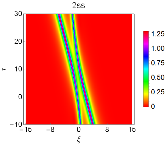
Figure 5: Interaction of 2 solitons moving with a relative velocity and having parameters $a_{1}=1$, $a_{2}=2$, $k_{1}=2$,$k_{2}=3$, $\alpha_{1}=1+i$, $\alpha_{2}=3+2i$ and $\beta=1+3i$.

Notice that the amplitude of soliton $q_{1}$ evaluated from eq. 29 and eq. 33 are found to be same. Similarly the amplitude of soliton $q_{2}$ evaluated from eq. 30 and eq. 34 are found to be same. That is the amplitude of solitons before and after interaction remain same, which is one of the important characteristics of soliton. However, the position of each soliton changes as a result of interaction, as evident from the figure 5. The same can be calculated from expressions in eqs. 29,  33 and eqs. 30, 34 and the magnitude of shift is given by

$$|\Delta_{ph}|=ln(\frac{(a_{1}-a_{2})^{2}+(k_{1}-k_{2})^{2}}{(a_{1}+a_{2})^{2}+(k_{1}-k_{2})^{2}})$$ (35)

Indeed, the phase shifts are opposite to each other.

Proceeding in a similar way, $N$-soliton solution is obtained by dropping terms of order greater than or equal to $\epsilon^{2N+1}$ in eqs. 11 - 13, which is

$$q=\frac{\epsilon g_{1}+\epsilon^{3}g_{3}+.....+\epsilon^{2N-1}g_{2N-1}}{f_{0}+\epsilon^{2}f_{2}+.....+\epsilon^{2N}f_{2N}}\Big{|}_{\epsilon=1}$$ (36)

where $g_{i}$, $f_{i}$ and $s_{i}$ are expanded as prescribed in [26, 27].

In the next section we will show the existence of infinite conserved quantities for the integrable FLE.

4 Conserved Quantities

In order to establish integrability in the Liouville sense, that is to compute the infinite number of conserved quantities we first find the Riccati equation from the Lax equation. The linear transformation equation for FLE in terms of Lax pair is given by

$$\partial_{\xi}{\bf\Psi}=L{\bf\Psi}$$ (37)

$$\partial_{\tau}{\bf\Psi}=M{\bf\Psi}$$ (38)

where $\bf{\Psi}$ is a two component vector field, expressed as

$${\bf\Psi}=({\Psi_{1}}\ {\Psi_{2}})^{T}$$ (39)

and $L$ and $M$ are given by

$$L=\frac{-i\zeta^{a}}{2}\ \Sigma+\zeta^{b}\ \partial_{\xi}u$$ (40)

$$M=\frac{i}{2}\zeta^{c}\ \Sigma-{i}{\zeta^{d}}\ \Sigma u+i\Sigma u^{2}$$ (41)

where $\zeta$ is the spectral parameter. To satisfy the zero curvature condition, namely

$$L_{\tau}-M_{\xi}+[L,M]=0$$ (42)

the exponents of $\zeta$, namely $a,\ b,\ c,\ d$ should satisfy the following relations,

$$a=b-d;\quad 2d=c;\quad b=-d$$ (43)

$\Sigma$ and $u$ are $2\times 2$ matrices, defined as follows

$\quad\Sigma=\left(\begin{tabular}[]{c c}1&0\\ 0&-1\\ \end{tabular}\right),\quad\quad u=\left(\begin{tabular}[]{c c}0&$q$\\ $-q^{*}$&0\\ \end{tabular}\right)$

Writing the first Lax eq. 40 in component form.

$$\Psi_{1\xi} =\frac{-i\zeta^{2}}{2}\Psi_{1}+\zeta\ q_{\xi}\ \Psi_{2}$$ (44)

$$\Psi_{2\xi} =\frac{i\zeta^{2}}{2}\Psi_{2}-\zeta\ q_{\xi}^{*}\ \Psi_{1}$$ (45)

Now following a similar procedure as in [24] we write

$$\Gamma=\frac{\Psi_{1}}{\Psi_{2}}$$ (46)

Then from eqs. 44, 45 we obtain a first order nonlinear differential equation,

$$\Gamma_{\xi}=-i\zeta^{2}\Gamma+\zeta q_{\xi}+\zeta q_{\xi}^{*}\Gamma^{2}$$ (47)

which is known as Riccati equation. The solution of the Riccati eq. 47 is related to the conserved quantities in the following way,

$$ln(a_{22}(\zeta))=ln(e^{-i\frac{\zeta^{2}}{2}\xi}\Psi_{2})|_{\xi\rightarrow\pm\infty}=-\zeta\int_{-\infty}^{\infty}q_{\xi}^{*}\Gamma\ d\xi=\sum_{n=0}^{\pm\infty}i^{n}H_{n}\zeta^{-n+1}$$ (48)

In eq. 48, $a_{22}$ is the scattering parameter and is time independent. In the summation, the negative powers of $\zeta$ give positive hierarchy $H_{n}$, where as the positive powers of $\zeta$ give negative hierarchy $H_{-n}$.
Consider the eq. 47 has a series solution,

$$\Gamma=\sum_{n=0}^{\infty}a_{\pm n}\zeta^{\mp n}$$ (49)

Substituting $\Gamma$ in eq. 47 we obtain the coefficients $a_{n}$;

$$a_{0} =0;\quad a_{1}=-i\partial_{\xi}q$$ (50)

$$a_{2} =0;\quad a_{3}=q_{\xi\xi}+i|q_{\xi}|^{2}q_{\xi}$$ (51)

$$a_{4} =0;\quad a_{5}=i(q_{\xi\xi\xi}-2|q_{\xi}|^{4}q_{x})-4|q_{\xi}|^{2}q_{\xi\xi}-(q_{\xi})^{2}q_{\xi\xi}^{*}$$ (52)

$$\cdots\qquad\cdots\qquad\cdots\qquad\cdots$$

$$a_{-1} =q;\quad a_{-2}=0;\quad a_{-3}=\int_{-\infty}^{\infty}(-iq+q^{2}q^{*}_{\xi})d\xi$$ (53)

$$\cdots\qquad\cdots\qquad\cdots\qquad\cdots$$

The conserved quantities thus obtained are

$$H_{1} =\int_{-\infty}^{\infty}|q_{\xi}|^{2}d\xi$$ (54)

$$H_{3} =\int_{-\infty}^{\infty}(|q_{\xi}|^{4}-iq_{\xi}^{*}q_{\xi\xi})d\xi$$ (55)

$$H_{5} =\int_{-\infty}^{\infty}(-q_{\xi}^{*}q_{\xi\xi\xi}+2|q_{\xi}|^{6}-3i|q_{\xi}|^{2}q_{\xi}^{*}q_{\xi\xi})d\xi$$ (56)

$$\cdots\qquad\cdots\qquad\cdots\qquad\cdots$$

$$\cdots\qquad\cdots\qquad\cdots\qquad\cdots$$

$$H_{-1} =\int_{-\infty}^{\infty}-iq_{\xi}^{*}q\ d\xi$$ (57)

$$H_{-3} =\int_{-\infty}^{\infty}-(|q|^{2}+i|q|^{2}qq_{\xi}^{*})\ d\xi$$ (58)

$$\cdots\qquad\cdots\qquad\cdots\qquad\cdots$$

$$\cdots\qquad\cdots\qquad\cdots\qquad\cdots$$

The negative indexed conserved quantities, namely eqs. 57, 58 are the members of negative hierarchy.

5 Conclusion

We have bilinearized Fokas-Lenells equation(FLE) with a vanishing boundary condition. In the proposed bilinearization we have used an auxiliary function to convert the trilinear equations into a set of bilinear equations. We have derived bright $1$-soliton, $2$- soliton solutions and presented the scheme for obtaining $N$- soliton solution. The additional parameter present in the soliton solution allows us to tune the position of soliton. We have shown that with a suitable choice of parameters one soliton solution reduces to an algebraic soliton. We have also shown explicitly through asymptotic analysis that the soliton interactions are elastic, that is the amplitude of each soliton before and after interaction are same. The mark of interaction is left behind only in the phase of each soliton. Secondly we have proposed a generalised Lax pair for the FLE and obtained the conserved quantities by solving the Riccati equation to establish the integrability in the Liouville sense. We feel that the proposed scheme of bilinearization considerably simplifies the procedure to obtain soliton solutions. We believe the present investigation would be useful to study the applications of FLE in nonlinear optics and other branches of physics.

References

- [1] Fokas, A. S. ”On a class of physically important integrable equations.” Physica D: Nonlinear Phenomena 87, no. 1-4 (1995): 145-150.
- [2] Lenells, Jonatan. ”Exactly solvable model for nonlinear pulse propagation in optical fibers.” Studies in Applied Mathematics 123, no. 2 (2009): 215-232.
- [3] Hasegawa, Akira, and Frederick Tappert. ”Transmission of stationary nonlinear optical pulses in dispersive dielectric fibers. I. Anomalous dispersion.” Applied Physics Letters 23, no. 3 (1973): 142-144.
- [4] Serkin, Vladimir N., and Akira Hasegawa. ”Novel soliton solutions of the nonlinear Schrödinger equation model.” Physical Review Letters 85, no. 21 (2000): 4502.
- [5] Kaup, David J., and Alan C. Newell. ”An exact solution for a derivative nonlinear Schrödinger equation.” Journal of Mathematical Physics 19, no. 4 (1978): 798-801.
- [6] Hirota, Ryogo, and Junkichi Satsuma. ”N-soliton solutions of model equations for shallow water waves.” Journal of the Physical Society of Japan 40, no. 2 (1976): 611-612.
- [7] Sasa, Narimasa, and Junkichi Satsuma. ”New-type of soliton solutions for a higher-order nonlinear Schrödinger equation.” Journal of the Physical Society of Japan 60, no. 2 (1991): 409-417.
- [8] Ahmed, Iftikhar, Aly R. Seadawy, and Dianchen Lu. ”M-shaped rational solitons and their interaction with kink waves in the Fokas–Lenells equation.” Physica Scripta 94, no. 5 (2019): 055205.
- [9] Arshad, Muhammad, Dianchen Lu, Mutti-Ur Rehman, Iftikhar Ahmed, and Abdul Malik Sultan. ”Optical solitary wave and elliptic function solutions of the Fokas–Lenells equation in the presence of perturbation terms and its modulation instability.” Physica Scripta 94, no. 10 (2019): 105202.
- [10] Hendi, Awatif A., Loubna Ouahid, Sachin Kumar, S. Owyed, and M. A. Abdou. ”Dynamical behaviors of various optical soliton solutions for the Fokas–Lenells equation.” Modern Physics Letters B 35, no. 34 (2021): 2150529.
- [11] Zhao, Yi, and Engui Fan. ”Inverse scattering transformation for the Fokas-Lenells equation with nonzero boundary conditions.” Journal of Nonlinear Mathematical Physics 28 no. 1 (2021): 38-52
- [12] Krishnan, E. V., Anjan Biswas, Qin Zhou, and Mohanad Alfiras. ”Optical soliton perturbation with Fokas–Lenells equation by mapping methods.” Optik 178 (2019): 104-110.
- [13] Cinar, Melih, Aydin Secer, Muslum Ozisik, and Mustafa Bayram. ”Derivation of optical solitons of dimensionless Fokas-Lenells equation with perturbation term using Sardar sub-equation method.” Optical and Quantum Electronics 54, no. 7 (2022): 402.
- [14] Matsuno,Yoshimasa. ”A direct method of solution for the Fokas–Lenells derivative nonlinear Schrödinger equation: I. Bright soliton solutions.” Journal of Physics A: Mathematical and Theoretical 45, no. 23 (2012): 235202.
- [15] Matsuno, Yoshimasa. ”A direct method of solution for the Fokas–Lenells derivative nonlinear Schrödinger equation: II. Dark soliton solutions.” Journal of Physics A: Mathematical and Theoretical 45, no. 47 (2012): 475202.
- [16] Agrawal, Govind P. Nonlinear Fiber Optics 3 (2013).
- [17] Kivshar, Yuri S., and Govind P. Agrawal. Optical solitons: from fibers to photonic crystals. Academic press, (2003).
- [18] Serkin, Vladimir N., and Akira Hasegawa. ”Exactly integrable nonlinear Schrodinger equation models with varying dispersion, nonlinearity and gain: application for soliton dispersion.” IEEE Journal of selected topics in Quantum Electronics 8, no. 3 (2002): 418-431.
- [19] Das, Ashok. Integrable models. Vol. 30. World scientific, (1989).
- [20] Al-Ghafri, K. S., E. V. Krishnan, and Anjan Biswas. ”W-shaped and other solitons in optical nanofibers.” Results in Physics 23 (2021): 103973.
- [21] Biswas, Anjan, Yakup Yıldırım, Emrullah Yaşar, Qin Zhou, Seithuti P. Moshokoa, and Milivoj Belic. ”Optical soliton solutions to Fokas-lenells equation using some different methods.” Optik 173 (2018): 21-31.
- [22] Triki, Houria, and Abdul-Majid Wazwaz. ”Combined optical solitary waves of the Fokas—Lenells equation.” Waves in Random and Complex Media 27, no. 4 (2017): 587-593.
- [23] Aljohani, A. F., E. R. El-Zahar, A. Ebaid, Mehmet Ekici, and Anjan Biswas. ”Optical soliton perturbation with Fokas-Lenells model by Riccati equation approach.” Optik 172 (2018): 741-745.
- [24] Ghosh, Sasanka, Anjan Kundu, and Sudipta Nandy. ”Soliton solutions, Liouville integrability and gauge equivalence of Sasa Satsuma equation.” Journal of Mathematical Physics 40, no. 4 (1999): 1993-2000.
- [25] Li, Yihao, Xianguo Geng, Bo Xue, and Ruomeng Li. ”Darboux transformation and exact solutions for a four-component Fokas–Lenells equation.” Results in Physics 31 (2021): 105027.
- [26] Nandy, Sudipta, and Abhijit Barthakur. ”Dark-bright soliton interactions in coupled nonautonomous nonlinear Schrödinger equation with complex potentials.” Chaos, Solitons & Fractals 143 (2021): 110560.
- [27] Nandy, Sudipta, and Abhijit Barthakur. ”Pairwise three soliton interactions, soliton logic gates in coupled nonlinear Schrödinger equation with variable coefficients.” Communications in Nonlinear Science and Numerical Simulation 69 (2019): 370-385.
- [28] Chakraborty, Sushmita, Sudipta Nandy, and Abhijit Barthakur. ”Bilinearization of the generalized coupled nonlinear Schrödinger equation with variable coefficients and gain and dark-bright pair soliton solutions.” Physical Review E 91, no. 2 (2015): 023210.