A method for automated regression test in scientific computing libraries: illustration with SPHinXsys

Abstract

Scientific computing libraries, either being in-house or open-source, have experienced enormous progress in both engineering and scientific research. It is therefore essential to ensure that the modifications in the source code aroused by bug fixing or new feature development wouldn’t compromise the accuracy and functionality that has already been validated and verified. With this in mind, this paper introduces a method for developing and implementing an automatic regression test environment and takes the open-source multi-physics library SPHinXsys [1] as an example. Firstly, the reference database for each benchmark test is generated from monitored data by multiple executions. This database contains the maximum variation range of metrics for different types of strategies, i.e., time-averaged method, ensemble-averaged method as well as the dynamic time warping method, covering the uncertainty arising from parallel computing, particle relaxation, physical instabilities, etc. Then, new results obtained after source code modification will be tested with them according to a curve-similarity based comparison. Whenever the source code is updated, the regression test will be carried out automatically for all test cases and used to report the validity of the current results. This regression test environment has already been implemented in all dynamics test cases released in SPHinXsys, including fluid dynamics, solid mechanics, fluid-structure interaction, thermal and mass diffusion, reaction-diffusion, and their multi-physics coupling, and shows good capability for testing various problems. It’s worth noting that while the present test environment is built and implemented for a specific scientific computing library, its underlying principle is generic and can be applied to many others.

1 Introduction

The development of computers has pushed scientific computing to become an indispensable part of many technologies and industries, such as in assessing climate change [2], designing new energy conductors [3], and imposes an ever-widening effect on better predicting and understanding the phenomena of nature and engineered systems. Following the definition of validation and verification of scientific computing claimed by William [4], scientific computing should always represent the real world and the conceptual model accurately. However, this is a challenging task due to the complex mathematical models and calculations, which often require changes to separate parts of the application and definitely increase the possibility of errors. Moreover, the development of scientific applications is a lasting work, and changes occur frequently due to different requirements and new features introduced. The applications should always produce trustworthy results and assure the application qualities with the help of validation and verification conducted alongside both application development and usage [5].

Implementing testing, including unit test, integration test, regression test, system test, etc., can provide concrete validation and verification procedures. Notwithstanding the fact that it has already been adopted in many IT software, scientific applications, especially some open-source libraries, find it difficult to perform those testing directly with traditional techniques. One main challenge is due to the characteristics of the scientific application, as it’s hard to find a test oracle to check if the program can gain the expected output when executing test cases [6, 7]. Another challenge arises from cultural differences between scientists and the software engineering community [6]. Many scientific applications are usually developed by small-group scientists, who may not be very familiar with accepted software engineering practices, and haven’t studied the developing process of their software in much detail [8], and therefore may overlook the impact of changes.

Regression test stands a great chance to ensure the output validity of scientific applications under development. It is a re-testing activity, which refers to executing the test suite with given inputs and comparing the output with previously stored reference results when modifications occur or new features are added. In this way, developers can make sure that their changes don’t cause any unexpected side effects and previous functionalities are still verified [7]. Since taking the regression test for all test cases is generally regarded as time-consuming and tedious for large-scale software, different automatic regression test techniques have already been successfully developed and implemented to alleviate this drawback, including selection [9, 10], minimization [11, 12], prioritization [13, 14], or optimization of test cases in the test suite.

Concerning the implementation of the regression test in scientific computing libraries, different focuses are of interest, for example, rigorous validation and verification are taken into account to be confident with the computational result. Therefore, different strategies should be followed and those processes should be automated and continuous [5]. Lin et al. [15, 16] have adopted historical data of multiple inputs and their relationships to define test oracle and then conduct the metamorphic test. Peng et al. [17, 18] reported their analysis regarding released unit tests and regression tests of SWMM, a stormwater management model developed by the U.S. Environmental Protection Agency. They focused on the test coverage and reveal an immature new pattern to mitigate the oracle problems. Farrel et al. [5] built an automated verification test environment for Fluidity-ICOM, which is an adaptive-mesh fluid dynamics simulation package. An web-based automated testing environment has also been developed by Liu et al. [19] to conduct the validating test for their computational fluid dynamics (CFD) cases related to high-speed aero-propulsive flows. Happ [20] developed a set of Linux C-Shell testing scripts for SHAMRC, a 2D and 3D finite-difference CFD code solving airblast-related problems, and run the regression test daily.

Despite the above-mentioned attempts of introducing testing in mesh-based scientific libraries, building a testing environment for meshless libraries is still absent even though more and more meshless computing libraries have been released and obtained more and more attraction. Actually, we encountered several instances when updating the source code of the SPHinXsys, an open-source multi-physics library developed by our group, that one or several test cases that passed the CTest(CMake Test)[21], but unexpectedly lead to the crash of simulations without any error output. We have believed that such cases were correct as they passed the tests, but in reality, they fall into fault. This issue is troublesome and has become the main motivation to build an effective regression test environment.

In this paper, a methodological framework for building an automatic regression test environment is introduced. Firstly, the verified reference database for each test case is generated according to adopting different types of monitoring data and stored as the reference. Then, the results obtained by the new version code will be tested with the reference database according to a curve-similarity based comparison. Updating the source code will activate the regression test automatically for each test case and report the validation of the result. Such a regression test scheme has already been implemented for all test cases released in SPHinXsys, covering different features. To the best knowledge of the authors, there is pioneering work in the regression test for open-source scientific computing libraries based on the meshless method. This work may also draw some attention from the general scientific computing communities to emphasize testing, because if the software is meant to do something, then that can and should be tested [22]. It’s worth noting that the principle presented in this work is versatile and can also be adopted in other scientific computing libraries. In what follows, Section 2 provides information about SPHinXsys and how tested data is obtained; Section 3 shows an overview of the regression test procedure as well as the detailed algorithm of three testing strategies; Section 4 introduces the environment set up and Section 5 illustrates several implementation examples in SPHinXsys. Finally, Section 6 concludes and puts forward future works.

2 Background

In this section, the feature of the SPHinXsys library is briefly introduced, and then the method for obtaining different tested data is also explained.

2.1 SPHinXsys

As a fully Lagrangian meshless method, smoothed particle hydrodynamics (SPH) was originally proposed for astrophysical applications [23, 24], and has been applied in simulating a great variety of scientific problems. SPHinXsys is an open-source multi-physics and multi-resolution scientific computing library [1] based on SPH, aiming at solving complex industrial and scientific applications. The current released version has several important features, such as dual-criteria time-stepping, spatio-temporal discretization, multi-resolution, position-based Verlet time-stepping scheme, etc., and could efficiently model and solve complex systems including fluid dynamics [25, 26], solid mechanics [27], fluid-solid interaction (FSI) [28], thermal and mass diffusion [29], reaction-diffusion [29], and electromechanics [29], etc. For quantitative validation, it contains more than 80 test cases where the analytical solution, experimental data, or numerical results from the literature are available for comparison. Note that several other open-source scientific libraries based on SPH have also been developed and released for public users. They all make valuable contributions to the SPH community, and their features have been described in the literature, such as GPUSPH [30], SPHysics [31], DualSPHysics [32], AQUAgpushp [33], GADGET-2 [34], and GIZMO [35]. The majority of those open-source scientific applications/libraries, including SPHinXsys, are still under intensive development. Therefore, it is essential to introduce a regression test environment for consistent development and release.

2.2 Obtaining tested data

For the majority of scientific computing problems, it is uncommon to obtain a database for the computational domain, since monitoring variables of interest at some typical locations are already able to provide a good reference. A variable of interest is usually called a variation point and its potential values in different executions are called variants [36]. As an example, in CFD simulations, the pressure probed at a fixed position can be a variation point and its values at a specific physical time for different executions are variants. By combining the variation point and variants with their constraints, a variability model can be generated from a series of computing results and provide references for the regression test.

In SPHinXsys, the monitoring data, also known as the variation point, can be classified into two types. One is the observed quantity at probes located within the computational domain. This includes variables such as density, pressure, velocity, etc., in fluid problems, and deformation, stress, displacement, etc., in solid, and other representative variables of interest. Another is the reduced quantity, which represents the overall variables of interest in the computational domain, such as summation, maximum, and minimum values of a variable, e.g., the total mechanical energy of the field. Note that these two types of quantities not only serve as the data source for the regression test but also for visualization.

3 Methodology

In this section, the overview of the regression test procedure will be introduced first, and then the individual steps and algorithms for three testing strategies are detailed follow.

3.1 Overview of the regression test

The underlying principle of the regression test is to compare the similarity between the verified curves (or time series results) generated from the previously verified executions in the reference database and the newly obtained ones after code modification. A verified curve usually includes a tolerance range due to the uncertainty induced in executions. For example, the concurrent vector is widely used in the shared memory parallel programming library, such as the Threading Building Blocks (TBB) library, to construct a sequence container with the feature of being concurrently grown and accessed. However, the results of multiple executions with the same model may not be exactly the same, but with noticeable or even considerable differences, especially for highly non-linear problems such as fluid dynamics.

In general, the regression test, as shown by the flow chart in Fig. 1,

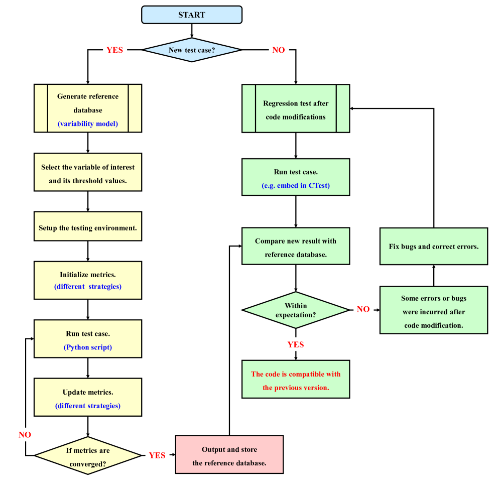
Figure 1: The flow chart for the regression test. The left part is for generating the reference database, and the right is for testing the new result obtained after code modification.

includes two parts: 1) a reference database for each test case is generated; 2) the new result after code modifications is checked automatically following specific strategies.

For a newly added test case, the following steps can be followed to generate a reference database:

1. Step 1: Execute the test case and verify the current result with experimental, numerical, or analytical data from the literature.

2. Step 2: Select one or more variables of interest and define the corresponding thresholds.

3. Step 3: Set up the testing environment by instantiating objects and introducing methods for the regression test, etc.

4. Step 4: Choose and initialize metrics from different strategies according to the type of generated curves or monitored time series results. Three different strategies, as explained in the following sections 3.3 - 3.5, are applied in this work.

5. Step 5: Execute the test case multiple times and update metrics with different strategies.

6. Step 6: Until the variations of all metrics are converged under the given threshold, the reference database will be stored.

Having the reference database in hand, the modified code can be tested as following steps:

1. Step 1: Run the test case by using the CMake Test or other similar testing packages.

2. Step 2: Compare the newly obtained result with the previously reserved one in the reference database based on curve-similarity measures.

3. Step 3: Check whether the similarity measure is within the given threshold. If it is, the modified code is considered to be acceptable. Otherwise, the source code should be checked for bugs. Then, the testing will be conducted again until the similarity measure is considered as acceptable.

3.2 Curve classification and testing strategies

Different strategies should be adopted for comparing curve similarity regarding various types of curves. For the typical dynamic problems considered in this work, the curves of time series data can be generally classified into three types, each corresponding to a different comparison strategy.

The first type, corresponding to the time-averaged strategy, represents data series that fluctuate around a constant value after reaching steady-state.

       

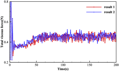
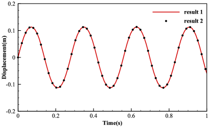
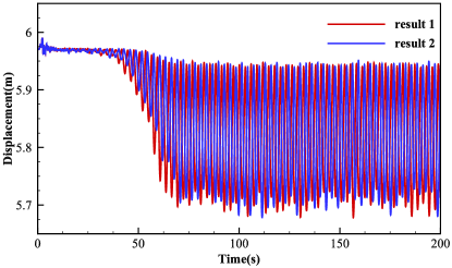
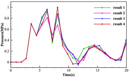
Figure 2: Different types of curves obtained from time series results and used for the regression test. (a) Type 1: total viscous force of the flow around cylinder [28]; (b) Type 2: free end displacement of an oscillating elastic beam [37]; (c) Type 3: flow-induced free end displacement of an elastic beam attached to a cylinder [28]; (d) Type 3: solid wall impacting pressure in dambreak flow [25, 26].

This kind of curve is prevalent in many fluid dynamics problems, such as the observed total viscous force for an fluid-structure interaction (FSI) problem, as illustrated in Figure 2. The second type, corresponding to the ensemble-averaged strategy, represents data series that exhibit similar variation patterns for each computing. Such curves are often generated from simple solid dynamics problems, such as the displacement of a given point from the oscillating beam presented in Figure 2. The last type, corresponding to the dynamic time warping (DTW) strategy, represents data series that may experience rapid and scattered variation patterns or large high-frequency fluctuation. Such curves are generally produced in simulations characterized by high nonlinear dynamics. Figure 2 displays a monitored position from an FSI simulation, and Figure 2 shows monitoring pressure for dambreak flow, both of which experience obvious variations in each execution.

3.3 Time-averaged strategy

In the time-averaged strategy, since the result always enters a steady state due to the relaxation process, the time-averaged mean and variance are used as metrics for comparison and testing.

3.3.1 Metrics generation and updating

The generation of the reference database under this strategy involves updating the time-averaged mean and variance through multiple executions until their variations converge. For each updating (e.g., the $n$th execution), the mean $M^{n}$ and variance $\sigma^{n}$ of the obtained result $x$ from the current execution can be calculated respectively as

$$\begin{cases}\displaystyle M^{n}=\frac{1}{l-k}\sum_{i=k}^{l}x_{i}^{n}\\ \displaystyle\sigma^{n}=\frac{1}{l-k}\sum_{i=k}^{l}\left(x_{i}^{n}-M^{n}\right)^{2}\end{cases},$$ (1)

where $i$ is the index of a data point, $l$ is the total number of data points, and $k$ is the index of the start point of the steady state. Then, the mean $M^{*}$ and variance $\sigma^{*}$ in the regression test metrics are updated based on the results from $n$th computations. Specifically, $M^{*}$ is updated as

$$M^{*}=\left(M^{n}+M^{*}\times\left(n-1\right)\right)/n.$$ (2)

Note that, instead of storing all previous mean $n$ times, the summation of the mean is recursively updated as a decaying average of all previous means for more efficiency. $\sigma^{*}$ is updated as

$$\sigma^{*}=\max\left(\sigma^{n},\sigma^{*}\right),$$ (3)

indicating that the variance is always updated to the maximum variation range. After the relative difference between the newly updated metrics and the previous ones is smaller than thresholds in several successive executions(usually 4), the $M^{*}$ and $\sigma^{*}$ are stored as the reference database. It is worth noting that the variation of the metrics of the two successive runs being smaller than the threshold is only a hint of convergence, so such should happen several times successively to ensure a real stable convergence. Therefore, once such variation is larger than the threshold, the counting of the converged successive executions will be reset as zero.

3.3.2 Start point searching

As the large oscillatory result in the early stage is nonphysical and can’t accurately reflect the real physical state of interest, this portion of data should be excluded. Here, a searching technique is proposed to locate the start point of the steady state, ensuring a reliable calculation of mean value and variance. Specifically, the search begins from the end of the time series as the simulation time is always set to be sufficiently long to ensure a steady state. To achieve this, $n$ pieces with the same time interval are sampled from the entire data, and, beginning from the end, two successive pieces are averaged separately and compared.

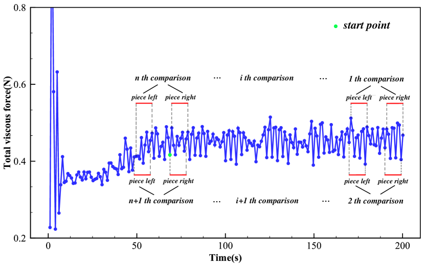
Figure 3: Schematic illustration of the start point searching technique.

As shown in Fig. 3, the comparison will proceed until the difference between two averages is larger than the given threshold.

Input: The current result $Array$ and its length $l$

Output: The index of the start point: $k$

1 Number of data points in each piece: $n=l/20$;

2 for $i=L-1$; $i\neq 3\times n$; $--i$ do

3       $M_{1}=0$, $M_{2}=0$;

4       for $j=i$; $j\neq i-n$; $--j$ do

5             $M_{1}\mathrel{+}=Array[j]/n$;

6             $M_{2}\mathrel{+}=Array[j-2\times n]/n$;

7            

8       end for

9      if $\lvert\left(M_{1}-M_{2}\right)/\left(M_{1}+M_{2}\right)\rvert\geq\rm{Threshold}$ then

10             $k=\max\left(k,i-n\right)$;

11             $break$;

12            

13       end if

14      

15 end for

Algorithm 1 : Search start point

The earliest pieces will be regarded as the start point of steady state. The detailed procedure is given in Algorithm 1

3.3.3 Regression test

For the regression test, the mean value and variance of the new result are compared with the metrics of the reference database. If the following conditions

$$\begin{cases}\lvert M-M^{*}\rvert\leq\alpha M^{*}\\ \sigma\leq\sigma^{*}\end{cases}$$ (4)

are satisfied, the new result is considered correct and the modified code is compatible with the previous version. Here, the parameter $\alpha$ is chosen according to different types of dynamics problems, and $\alpha=0.05$ for solid dynamics and $\alpha=0.1$ for fluid dynamics are applied in SPHinXsys.

3.4 Ensemble-averaged strategy

In the ensemble-averaged strategy, the result curves obtained from the simulation runs are often similar to each other with a variation range, which is defined by the metrics of ensemble-averaged mean and variance.

3.4.1 Metrics generation and updating

For the $n$th execution, the metrics for each data point $i$ are updated based on the previous values and the new results. The ensemble-averaged mean $M_{i}^{*}$ at a data point $i$ is updated as

$$M_{i}^{*}=\left(x_{i}^{n}+M_{i}^{n-1}\times\left(n-1\right)\right)/n.$$ (5)

where $x_{i}^{n}$ is the newly obtained data point and $M_{i}^{n-1}$ is the previous mean. Similar to the time-averaged strategy, the new variance $\sigma_{i}^{*}$ is updated as

$$\sigma_{i}^{*}=\max\left(\sigma^{*}_{i},\sigma_{i}^{n-1},\left(0.01*\left(M_{i,max}^{*}-M_{i,min}^{*}\right)\right)^{2}\right),$$ (6)

where the last term is a secure value that is introduced to create a variation range and prevent zero maximum variance for results from different computations. Such a secure value is set according to the maximum and minimum value of the local result. Again, the convergence criteria same as that in the time-averaged strategy, i.e. successive executions with sufficient small variations of the updated mean and variance are used to terminate the metrics updating.

3.4.2 Extreme value filter

In some cases, particularly in certain physical problems, there will be some obvious extreme values in otherwise smooth and regular results. These values are often obtained from fast events with insufficient sampling frequency, such as wave-impacting events within generally continuous FSI problems, and may negatively impact the accuracy of the metrics. Therefore, an extreme value filter is introduced and adopted in some test cases.

As shown in Algorithm 2,

Input: The current result $Array$ and its total length $l$

Output: The smoothed result $Filtered$

1 Length of each data segment: $n=l/200$;

2 for $i=0$; $i\neq l$; $++i$ do

3       $Filtered[i]=Array[i],M_{nbh}=0,\sigma_{nbh}=0,\sigma_{test}=0$;

4       for $j=\max\left(i-n,0\right)$; $j\neq\min\left(i+n,l\right)$; $++j$ do

5             calculate neighboring points mean $M_{nhb}$;

6       end for

7      for $j=\max\left(i-n,0\right)$; $j\neq\min\left(i+n,l\right)$; $++j$ do

8             calculate neighboring points variance $\sigma_{nhb}$;

9       end for

10      calculate tested point variance $\sigma_{test}=\left(Array[i]-M_{nbh}\right)^{2}$;

11       if $\sigma_{test}>4\times\sigma_{nhb}$ then

12             $Filtered[i]=M_{nhb}$;

13            

14       end if

15      

16 end for

Algorithm 2 Extreme value filter

the total dataset is decomposed into $n$ segments, and each contains one tested data point and its neighboring data points. Then, for each data segment, the standard variance of neighboring data points is compared with the variance of between the tested data and the neighboring data. If the latter is four times larger than the former, this tested data point will be considered an extreme value point and is reset to the mean of its neighboring data.

   

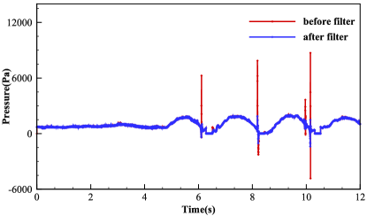
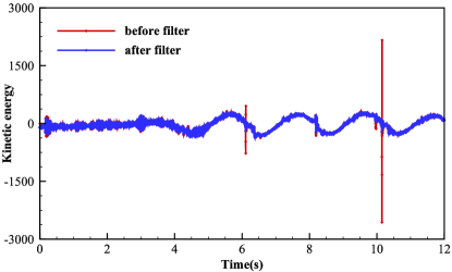
Figure 4: Extreme filtering in the problem oscillating wave surge converter [38]: (a) pressure at a probe; (b) total kinetic energy.

Fig. 4 presents the filtering of the pressure of a fixed position and total kinetic energy from the oscillating wave surge converter case [38].

3.4.3 Regression test

Having the metrics of the reference database in hand, the regression test after code modification will be carried out for all data points with the following condition

$$\sqrt{\left(x_{i}^{n}-M_{i}^{*}\right)^{2}}\leq\sigma_{i}^{*}.$$ (7)

If there is any data point that does not satisfy this condition, the code modification should be checked and corrected.

3.5 Dynamic time warping (DTW) strategy

DTW, which was originally proposed for spoken word recognition [39, 40], is a dynamic programming algorithm used to measure the similarity between two sequences with temporal variation by computing the DTW distance. Compared to the Euclidean distance, DTW is more accurate and can handle non-linear distortions, shifts, and scaling in the time dimension. It has been widely used in various research areas such as sign language recognition [41] and time-series clustering [42], etc. Additionally, this algorithm is also applied in many engineering fields involving time-series comparison, e.g., in health monitoring and fault diagnosis [43]. Actually, due to its generic properties, the DTW strategy may also be used for the curve types that are not classified in Section 3.2.

3.5.1 Calculation of DTW distance

Suppose we have two time series,

$$\begin{cases}P:p_{1},p_{2},\dots,p_{i},\dots,p_{m-1},p_{m}\\ Q:q_{1},q_{2},\dots,q_{j},\dots,q_{n-1},q_{n}\end{cases},$$ (8)

where $m$ and $n$ indicate the length of time series $P$ and $Q$, respectively. $i$ and $j$ are data point indices in the time series. The DTW algorithm divides the problem into multiple sub-problems, and each sub-problem contributes to the cumulative calculation of the distance [44]. The first step is to construct a local distance matrix $d$ consisting of $m\times n$ elements, where each element represents the Euclidean distance between two data points in the time series. Then, the warping matrix $D$, seen in Fig. 5,

   

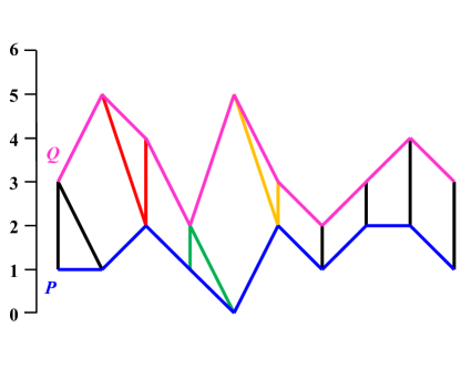
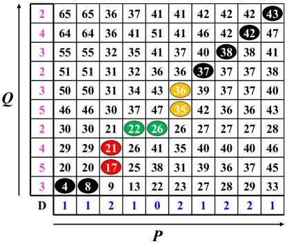
Figure 5: Illustration of the DTW. (a) Aligning measurements to calculate the DTW distance between two sequences, P and Q; (b) The warping matrix D generated by DTW; labeled cells represents the optimal warping path.

is filled based on

$$D(i,j)=d(i,j)+\min\begin{cases}D(i-1,j)\\ D(i-1,j-1)\\ D(i,j-1)\end{cases}.$$ (9)

Finally, DTW reports the optimal warping path and the DTW distance. The warping path consists of a set of adjacent matrix elements that identify the mapping between two sequences, representing the path that minimizes the overall distance between $P$ and $Q$. Each warping path should follow certain rules [39, 45, 46]: each index from the first sequence must be matched with one or more indices from the other sequence, and such mapping must be monotonically increasing. Note that the first index and the last index from the first sequence must be matched with their counterparts from the other sequence correspondingly.

However, DTW can be computationally expensive when searching for global matches, and as a result, many algorithms have been proposed to reduce futile computation [39, 46, 47, 48, 49]. One effective and simple method for speeding up DTW is to set a warping window(ww) [39]. The warping window adds a local constraint that forces the warping path to lie within a band around the diagonal, as shown in Fig. 6,

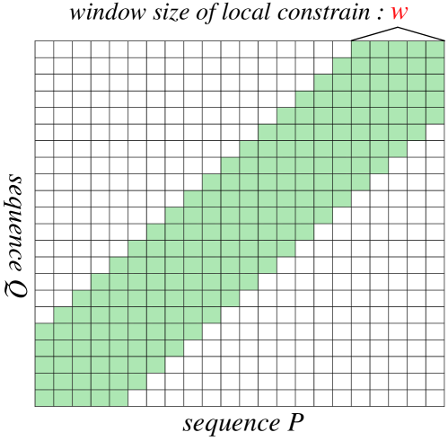
Figure 6: The warping scope limited by the warping window.

restricting the searching window to the fixed size $w$. In the current work, we adopt the window size $w$ as

$$w=\max\left(\lvert m-n\rvert,5\right).$$ (10)

After imposing the constraint, the warping will only occur within the diagonal green areas, and if the optimal path crosses the band, the distance will not be the optimal one.

3.5.2 Metrics generation and updating

The maximum DTW distance is used as the regression test metric and is updated after each execution until its variation converges to a certain threshold. With the initial value for the first computation set as $D_{0,0}=0$, the maximum distance for the $n$th execution will be calculated as

$$D^{*}=\max\left(D^{*},D_{0,n},D_{1,n},\dots,D_{n-2,n},D_{n-1,n}\right),$$ (11)

where the subscript, e.g., $D_{n-2,n}$ denote the distance between the $(n-2)$th and $n$th computational results. Similar to the other two strategies, after the variation of $D^{*}$ converges to a given threshold in successive several executions, the $D^{*}$ and several results (usually 3 $\sim$ 5) with all data points are stored for the regression test.

3.5.3 Regression testing

For the regression test, if the DTW distances between the new result after code modification and each result in the reference database are satisfied

$$\left(D_{1},D_{2},\cdots,D_{k}\right)\leq D^{*},k=3\sim 5,$$ (12)

the new result is regarded as acceptable, Otherwise, it is beyond expectation and the code should be checked and corrected.

4 Regression test environment

In this section, taking SPHinXsys as an example, the process of building an automatic regression test environment is explained. The test interface is integrated into a SPHinXsys application’s case code based on the data monitoring module. In SPHinXsys, the monitoring module includes two classes, as depicted in Fig. 7.

   

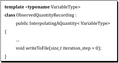
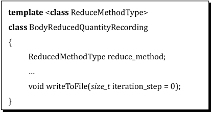
Figure 7: Monitoring methods in SPHinXsys: (a) observation of a variable of interest by ObservedQuantityRecording; (b) reducing the variable of interest by BodyReducedQuantityRecording.

The observed quantities at probes are generated from ObservedQuantityRecording, and the reduced quantities are obtained from BodyReducedQuantityRecording. The above two methods are implemented with the template, allowing the flexible handling of various data types, and also providing rich data sources for the regression test.

Fig. 8 presents the relationship among different regression test methods.

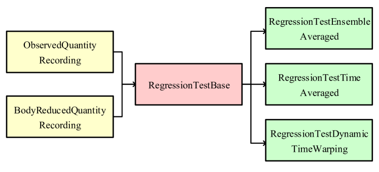
Figure 8: Relationship of classes related to the regression test in SPHinXsys.

The class template RegressionTestBase, defining commonly used methods in the regression test, inherits from the above monitoring class. Then, three derived template classes are defined to implement specialized methods, i.e., RegressionTestTimeAveraged, RegressionTestEnsembleAveraged as well as RegressionTestDynamicTimeWarping, respectively. Note that the present structure provides a very flexible combination of test strategies for various variables of interest.

To set up a regression test for a specific test case, it only needs to replace the existing monitoring class with the regression test class based on the type of curve that is being monitored. Afterward, call the interface generateDataBase() to generate a reference database or testNewResult() to perform a regression test at the end of the case file. It should be noted that the current method does not disturb the existing code structure. In the SPHinXsys package, a python script, as exampled in Fig. 9, is employed to execute a test case multiple times automatically for generating the reference database.

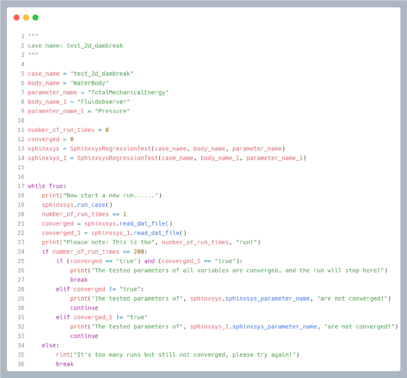
Figure 9: Example of the Python script for generating test metrics for a 2d dambreak flow case in SPHinXsys, with two variables of interest.

It is an automatic process as long as the script is made for the test case, and it is also easy to regenerate the reference database when it is necessary.

In SPHinXsys, the regression test is setup for all test cases which simulate real-world problems with SPH method. Together with Google test [50] for unit test, all tests are integrated using the CTest [21]. When merging of branches occurs, all tests can be triggered automatically.

5 Applications and examples

The obtained reference database for several test cases will be presented here to demonstrate the functionality of current regression test method.

5.1 Dambreak

The first example is the dambreak flow in two and three dimensions. The total mechanical energy of the entire domain and pressure at fixed probes have been recorded and validated [25, 37]. Thus, those two monitoring variables have been used for the regression test. According to the classification of curves, the ensemble-averaged strategy is used for the curve of total mechanical energy, and the DTW strategy is used for the pressure curve.

   

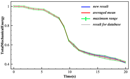
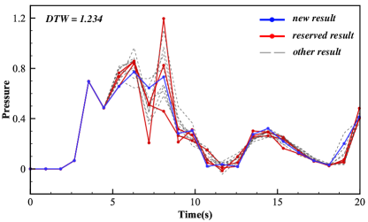
Figure 10: Illustration of the reference database and results for the 2d dambreak case: (a) total kinetic energy; (b) pressure.

       

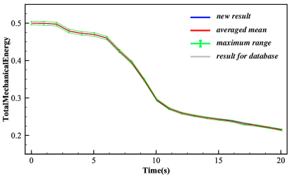
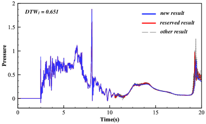
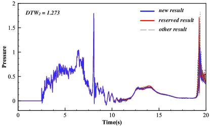
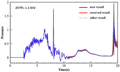
Figure 11: Illustration of reference database and results for the 3d dambreak case: (a) total kinetic energy; (b) pressure at probe a; (c) pressure at probe b; (d) pressure at probe c.

It is observed that the kinetic energies obtained after code modification, see Figs. 10 and 11, are within the range of reference database. The collection of multiple pressure results is given in Fig. 10 and 11 - 11, where the 3d case has three pressure monitoring points. After continuously updating the maximum DTW distances for each pair of results, the variation of distances converges, and the final distance is stored, as listed in Table 1. Actually, not all computational results but only several randomly chosen ones are shown here and have been reserved in the reference database.

Table 1: DTW distance in the reference database and for the new results.

DTW distance	2d	3d:probe a	3d:probe b	3d:probe c
database	$1.234$	$0.651$	$1.273$	$1.034$
testing1	$0.368$	$0.180$	$0.229$	$0.231$
testing2	$0.535$	$0.177$	$0.153$	$0.144$
testing3	$0.522$	$0.015$	$0.084$	$0.111$

Table 1 indicates that the distance between the newly obtained results and the ones stored in the database are all smaller than the reference distances. Therefore, after performing the regression test on those two variables, new results obtained after code modification are deemed correct, and the new code is considered to be compatible with the old version for the dambreak flow case.

5.2 Oscillating-beam

The second example is the free end oscillating elastic beam problem. The detailed setting up and validation can be referred in our previous work [37]. The displacement of the beam tip has been recorded and used for the regression test. This variable has two components representing different directions, and it has small differences for each computation, so the ensemble-averaged method is adopted for generating the reference database and new result testing. Fig. 12 demonstrates the reference database for this case.

   

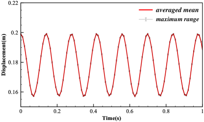
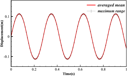
Figure 12: Illustration of the reference database and results for the 2d oscillating beam case: displacement along (a) $x$ direction, and (b) $y$ direction, respectively. The red lines represent the ensemble-averaged mean for each data point, and the gray ones gives the range of maximum variation.

It is found that the new result of this case (not shown here due to very small, not noticeable visually, differences) after code modifications lies within the range given by the reference database for each data point.

5.3 Fluid-solid interaction

The last example is a fluid-solid interaction problem on flow-induced vibration. More information as well as validations can be referred in earlier work [26, 28]. The total viscous force from the fluid acting on the solid structure was recorded, and it fluctuates around the constant value when the dynamics entered a periodic oscillation state. Thus, the time-averaged method is used to perform the regression test for this variable. Since the force in the $y$ direction is relatively small, only the $x$ direction force was considered. Fig. 13 displays the reference database and one tested new result for this case.

Figure 13: Illustration of the reference database and the tested result for the FSI problem. The gray dashed lines represent multiple results used for generating the database, and the red line is a new result after code modification. The green line shows the time-averaged mean of multiple results, and blue ones indicate the variation range constrained by the variance.

Table 2 shows the converged metric values in the database as well as the ones from the new result.

Table 2: Mean and variance in the reference database and for the new result.

metric	database	new result
mean	$0.4557$	$0.4549$
variance	$0.00173$	$0.00157$

It indicates the new mean is quite close to the converged one, and the new variance is also smaller than the reference one. Therefore, the new result of the FSI problem after code modification is still considered correct.

In general, each test case should have at least one variable of interest used for the regression test, and the testing strategy is not fixed. This regression test environment provides flexible combinations of variables and strategies, but each variable should always have the best option to check itself.

6 Conclusion

This paper introduces a method for developing an automatic regression test environment for open-source scientific libraries and uses SPHinXsys as an illustration to demonstrate its functionality. For scientific libraries under centralized development, it’s essential to guarantee the accuracy of simulation results all the time, and the regression test provides this procedure. The reference database for each benchmark test is generated using different strategies, and the new result after code modifications can be automatically tested with them once the source code is updated. This regression test environment has been implemented in all test cases released in SPHinXsys, and it shows great functionality to check the validity of the new result obtained after code modifications. By doing such work, we also want to drawn some attention from general scientific computing communities to emphasize the software performance during development. The principle of the regression test proposed here is universal and can be applied and extended in other libraries and applications. In the future, other regression test methods will be implemented, and with the number of test cases swelling due to adding new dynamics features, selection and reduction of test cases will also be adopted.

References

- [1] C. Zhang, M. Rezavand, Y. Zhu, Y. Yu, D. Wu, W. Zhang, J. Wang, X. Hu, Sphinxsys: An open-source multi-physics and multi-resolution library based on smoothed particle hydrodynamics, Computer Physics Communications 267 (2021) 108066.
- [2] J. B. Drake, P. W. Jones, G. R. Carr Jr, Overview of the software design of the community climate system model, The International Journal of High Performance Computing Applications 19 (3) (2005) 177–186.
- [3] D. E. Post, R. P. Kendall, Software project management and quality engineering practices for complex, coupled multiphysics, massively parallel computational simulations: Lessons learned from asci, The International Journal of High Performance Computing Applications 18 (4) (2004) 399–416.
- [4] W. L. Oberkampf, C. J. Roy, Verification and validation in scientific computing., Cambridge: Cambridge University Press, 2010.
- [5] P. Farrell, M. Piggott, G. Gorman, D. Ham, C. Wilson, T. Bond, Automated continuous verification for numerical simulation, Geoscientific Model Development 4 (2) (2011) 435–449.
- [6] U. Kanewala, J. M. Bieman, Testing scientific software: A systematic literature review, Information and software technology 56 (10) (2014) 1219–1232.
- [7] H. Remmel, B. Paech, P. Bastian, C. Engwer, System testing a scientific framework using a regression-test environment, Computing in Science & Engineering 14 (2) (2011) 38–45.
- [8] K. Bojana, Framework for developing scientific applications, Ph.D. thesis, UNIVERSITY SS CYRIL AND METHODIUS (2018).
- [9] H. Ural, H. Yenigün, Regression test suite selection using dependence analysis, Journal of Software: Evolution and Process 25 (7) (2013) 681–709.
- [10] A. P. Agrawal, A. Choudhary, A. Kaur, An effective regression test case selection using hybrid whale optimization algorithm, International Journal of Distributed Systems and Technologies (IJDST) 11 (1) (2020) 53–67.
- [11] D. Di Nardo, N. Alshahwan, L. Briand, Y. Labiche, Coverage-based regression test case selection, minimization and prioritization: A case study on an industrial system, Software Testing, Verification and Reliability 25 (4) (2015) 371–396.
- [12] S. Prasad, M. Jain, S. Singh, C. Patvardhan, Regression optimizer a multi coverage criteria test suite minimization technique, International Journal of Applied Information Systems (IJAIS) 1 (8).
- [13] S. Harikarthik, V. Palanisamy, P. Ramanathan, Optimal test suite selection in regression testing with testcase prioritization using modified ann and whale optimization algorithm, Cluster Computing 22 (5) (2019) 11425–11434.
- [14] L. Tahat, B. Korel, M. Harman, H. Ural, Regression test suite prioritization using system models, Software Testing, Verification and Reliability 22 (7) (2012) 481–506.
- [15] X. Lin, M. Simon, N. Niu, Exploratory metamorphic testing for scientific software, Computing in science & engineering 22 (2) (2018) 78–87.
- [16] X. Lin, M. Simon, N. Niu, Hierarchical metamorphic relations for testing scientific software, in: 2018 IEEE/ACM 13th International Workshop on Software Engineering for Science (SE4Science), IEEE, 2018, pp. 1–8.
- [17] Z. Peng, X. Lin, N. Niu, Unit tests of scientific software: A study on swmm, in: International Conference on Computational Science, Springer, 2020, pp. 413–427.
- [18] Z. Peng, X. Lin, M. Simon, N. Niu, Unit and regression tests of scientific software: A study on swmm, Journal of Computational Science 53 (2021) 101347.
- [19] Z. Liu, K. Brinckman, S. Dash, Automated validation of cfd codes for analysis of scramjet propulsive flows using crave, in: 45th AIAA/ASME/SAE/ASEE Joint Propulsion Conference & Exhibit, 2009, p. 4846.
- [20] H. J. Happ, Linux c-shell regression testing for the shamrc cfd code, in: Users’~ Group Conference, 2011, p. 41.
- [21] Kitware Inc. et al., CMake. https://cmake.org/documentation/, accessed on 7thJuly 2021.
- [22] R. Baxter, Software engineering is software engineering, in: 26th International Conference on Software Engineering, W36 Workshop Software Engineering for High Performance System (HPCS) Applications, IET, 2004, pp. 4–18.
- [23] L. B. Lucy, A numerical approach to the testing of the fission hypothesis, The astronomical journal 82 (1977) 1013–1024.
- [24] R. A. Gingold, J. J. Monaghan, Smoothed particle hydrodynamics: theory and application to non-spherical stars, Monthly notices of the royal astronomical society 181 (3) (1977) 375–389.
- [25] C. Zhang, X. Hu, N. A. Adams, A weakly compressible sph method based on a low-dissipation riemann solver, Journal of Computational Physics 335 (2017) 605–620.
- [26] C. Zhang, M. Rezavand, X. Hu, Dual-criteria time stepping for weakly compressible smoothed particle hydrodynamics, Journal of Computational Physics 404 (2020) 109135.
- [27] C. Zhang, Y. Zhu, Y. Yu, M. Rezavand, X. Hu, A simple artificial damping method for total lagrangian smoothed particle hydrodynamics, arXiv preprint arXiv:2102.04898.
- [28] C. Zhang, M. Rezavand, X. Hu, A multi-resolution sph method for fluid-structure interactions, Journal of Computational Physics 429 (2021) 110028.
- [29] C. Zhang, J. Wang, M. Rezavand, D. Wu, X. Hu, An integrative smoothed particle hydrodynamics method for modeling cardiac function, Computer Methods in Applied Mechanics and Engineering 381 (2021) 113847.
- [30] G. Bilotta, A. Hérault, A. Cappello, G. Ganci, C. Del Negro, Gpusph: a smoothed particle hydrodynamics model for the thermal and rheological evolution of lava flows, Geological Society, London, Special Publications 426 (1) (2016) 387–408.
- [31] M. Gomez-Gesteira, B. Rogers, A. Crespo, R. Dalrymple, M. Narayanaswamy, J. Dominguez, Sphysics – development of a free-surface fluid solver – part 1: Theory and formulations, Computers and Geosciences 48 (2012) 289–299.
- [32] A. J. Crespo, J. M. Domínguez, B. D. Rogers, M. Gómez-Gesteira, S. Longshaw, R. Canelas, R. Vacondio, A. Barreiro, O. García-Feal, Dualsphysics: Open-source parallel cfd solver based on smoothed particle hydrodynamics (sph), Computer Physics Communications 187 (2015) 204–216.
- [33] J. L. Cercos-Pita, Aquagpusph, a new free 3d sph solver accelerated with opencl, Computer Physics Communications 192 (2015) 295–312.
- [34] V. Springel, The cosmological simulation code gadget-2, Monthly notices of the royal astronomical society 364 (4) (2005) 1105–1134.
- [35] P. F. Hopkins, A new public release of the gizmo code, arXiv preprint arXiv:1712.01294.
- [36] K. Pohl, G. Böckle, F. Van Der Linden, Software product line engineering: foundations, principles, and techniques, Vol. 1, Springer, 2005.
- [37] C. Zhang, X. Y. Hu, N. A. Adams, A generalized transport-velocity formulation for smoothed particle hydrodynamics, Journal of Computational Physics 337 (2017) 216–232.
- [38] C. Zhang, Y. Wei, F. Dias, X. Hu, An efficient fully lagrangian solver for modeling wave interaction with oscillating wave surge converter, Ocean Engineering 236 (2021) 109540.
- [39] H. Sakoe, S. Chiba, Dynamic programming algorithm optimization for spoken word recognition, IEEE transactions on acoustics, speech, and signal processing 26 (1) (1978) 43–49.
- [40] C. Myers, L. Rabiner, A. Rosenberg, Performance tradeoffs in dynamic time warping algorithms for isolated word recognition, IEEE Transactions on Acoustics, Speech, and Signal Processing 28 (6) (1980) 623–635.
- [41] J. Cheng, F. Wei, Y. Liu, C. Li, Q. Chen, X. Chen, Chinese sign language recognition based on dtw-distance-mapping features, Mathematical Problems in Engineering 2020.
- [42] H. Li, J. Liu, Z. Yang, R. W. Liu, K. Wu, Y. Wan, Adaptively constrained dynamic time warping for time series classification and clustering, Information Sciences 534 (2020) 97–116.
- [43] A. C. Douglass, J. B. Harley, Dynamic time warping temperature compensation for guided wave structural health monitoring, IEEE Transactions on Ultrasonics, Ferroelectrics, and Frequency Control 65 (5) (2018) 851–861.
- [44] G. Al-Naymat, S. Chawla, J. Taheri, Sparsedtw: A novel approach to speed up dynamic time warping, arXiv preprint arXiv:1201.2969.
- [45] C. A. Ratanamahatana, E. Keogh, Everything you know about dynamic time warping is wrong, in: Third workshop on mining temporal and sequential data, Vol. 32, Citeseer, 2004.
- [46] S. Salvador, P. Chan, Toward accurate dynamic time warping in linear time and space, Intelligent Data Analysis 11 (5) (2007) 561–580.
- [47] E. Keogh, C. A. Ratanamahatana, Exact indexing of dynamic time warping, Knowledge and information systems 7 (2005) 358–386.
- [48] D. Lemire, Faster retrieval with a two-pass dynamic-time-warping lower bound, Pattern recognition 42 (9) (2009) 2169–2180.
- [49] Y. Sakurai, M. Yoshikawa, C. Faloutsos, Ftw: fast similarity search under the time warping distance, in: Proceedings of the twenty-fourth ACM SIGMOD-SIGACT-SIGART symposium on Principles of database systems, 2005, pp. 326–337.
- [50] J. A. Whittaker, J. Arbon, J. Carollo, How Google tests software, Addison-Wesley, 2012.