First-order phase transition between superconductivity and charge/spin-density wave as the reason of their coexistence in organic metals

Abstract

The interplay between superconductivity (SC) and spin/charge density wave (DW) in organic metals shows many similarities to high-$T_{c}$ superconductors. It also contains many puzzles, for example, the anisotropic SC onset observed and the severalfold increase of the upper critical field $H_{c2}$ in the coexistence region, as well as the microscopic origin of SC/DW phase separation there. In this paper, by the direct calculation of the Landau expansion for DW free energy, we argue that the phase transition between DW and metallic/SC phase in organic superconductors goes by first order at low enough temperature, which explains the spatial segregation of DW and SC at large length scale, consistent with experimental observations. This first-order phase transition is not directly related to SC and happens even above the SC transition temperature.

I Introduction

The properties of metals with a charge-density-wave (CDW) or spin-density-wave (SDW) ground state attract great attention since the fifties (see, e.g., [1, 2]). It often competes with superconductivity (SC) [3, 4, 2], e.g., in most high-$T_{c}$ superconductors, both cuprate [5, 6, 7, 8, 9, 10] and iron-based [11, 12], and remains a subject of active investigation in many other materials, including transition metal dichalcogenides [13, 14], organic superconductors (OS) [15, 16, 17, 18, 19, 20, 21, 22, 23, 24, 25, 26, 27] and even materials with nontrivial topology of band structures [28].

The OS are interesting for studying the interplay between CDW/SDW and SC because their phase diagram, layered crystal structure and many other features resemble those in cuprate and iron-based high-$T_{c}$ superconductors, but they are simpler and more convenient for investigation. By changing the chemical composition one can control the electronic dispersion in OS in a wide interval. One can grow rather large and pure monocrystals of organic metals, so that their electronic structure can be experimentally studied by high-magnetic-field tools [29]. Finally, the OS are simpler for theoretical study because of weaker electronic correlations [15, 16]. Therefore, the OS are very helpful for disentangling various factors affecting the electronic and superconducting properties, which is hard to do in cuprates and other strongly correlated materials. SC and DW coexist even in relatively weakly correlated OS, such as (TMTSF)₂PF₆ [21, 18, 19, 20], (TMTSF)₂ClO₄ [25, 26] or $\upalpha$-(BEDT-TTF)₂KHg(SCN)₄ [27]. In these materials the density wave (DW) is suppressed by some external parameter, such as pressure or cooling rate. Similar to cuprates, the SC transition temperature $T_{\text{cSC}}$ is the highest in the coexistence region near the quantum critical point where DW disappears. The upper critical field $H_{c2}$ is often several times higher in the coexistence region than in a pure SC phase [17, 27], the effect potentially useful for applications.

The microscopic structure of SC and DW coexistence is important for understanding the DW influence on SC properties and $T_{cSC}$. The DW and SC phase separation may happen in the momentum or coordinate space. The first scenario assumes a spatially uniform structure, when the Fermi surface (FS) is partially gapped by DW and the ungapped parts give SC [2, 30]. It is similar to most other CDW materials [2, 3, 4]. The second scenario assumes that SC and DW phases are spatially separated on a microscopic or macroscopic scale, depending on the ratio of SC domain size $d$ and the SC coherence length $\xi_{\text{SC}}$. The temperature resistivity hysteresis observed in (TMTSF)₂PF₆ [18] supports the spatial SC/DW separation. The width of SC transition increases with the increase of disorder, controlled by the cooling rate in (TMTSF)₂ClO₄, which also indicates a spatial SDW/SC segregation [26] similar to granular superconductors. The microscopic SC domains of width $d$ comparable to or even less than the SC coherence length $\xi_{\text{SC}}$ may appear in the soliton DW structure, where SC emerges inside the soliton walls [31, 32, 33, 34, 35, 33]. However, the angular magnetoresistance oscillations inside the parametric region of SC/DW coexistence observed in (TMTSF)₂PF₆ [20] and in (TMTSF)₂ClO₄ [24] seem to be consistent with only a macroscopic spatial phase separation with SC domain width $d>1$ µm. The SC upper critical field $H_{c2}$ may theoretically exceed several times the $H_{c2}$ without DW coexistence in all the above scenarios [30, 33], provided the SC domain width is smaller or comparable to the penetration depth $\lambda$ of magnetic field to the superconductor.

The puzzling feature of SDW/SC coexistence in (TMTSF)₂PF₆, long unexplained in any scenario, is the anisotropic SC onset [19, 20]: with the increase in pressure at $P=P_{c2}\approx 6.7$ kbar the SC transition and the zero resistance is first observed only along the least-conducting interlayer $z$-direction, then at $P=P_{c1}\approx 7.8$ kbar along $z$- and $y$-directions, and only at $P=P_{c0}\approx 8.6$ kbar in all directions, including the most conducting $x$-direction. This is opposite to a weak intrinsic interlayer Josephson coupling, typical in high-$T_{c}$ superconductors [36]. Other organic metals manifest similar anisotropic SC onset in the region of coexistence with DW [25]. The observed [19, 20, 25] anisotropic zero-resistance transition temperature $T_{\text{cSC}}$ seems to contradicts the general rule that the percolation threshold in macroscopic heterogeneous media must be isotropic [37], provided the SC inclusions are not thin filaments [19] connecting opposite edges of a sample. However, such a filament scenario cannot be substantiated microscopically, neither in (TMTSF)₂PF₆ nor in (TMTSF)₂ClO₄. This paradox was resolved recently [38, 39] by assuming a spatial SC/DW separation and studying the percolation in finite-size samples of the thin elongated shape, relevant to the experiments in (TMTSF)₂PF₆ [19, 20] and (TMTSF)₂ClO₄ [25, 26]. Similar effect was observed and used to study the SC domain shape and size in other superconductors, for example, in FeSe [40, 41, 42] or other organic metals [43]. This supports the scenario of spatial SC/DW segregation in a form of rather large domains of width $d>1$ µm in organic superconductors. However, the microscopic reason for such phase segregation remains unknown and is the main goal of our study.

In this paper we argue that the phase transition between DW and metallic/SC phase in OS goes by first order at low enough temperature, which explains the spatial segregation of DW and SC at large length scale, consistent with experimental observations. This first-order phase transition is not directly related to SC and happens even at $T>T_{\text{cSC}}$ because of the suppression of DW by the deterioration of FS nesting, which is controlled by pressure in (TMTSF)₂PF₆ and in $\upalpha$-(BEDT-TTF)₂KHg(SCN)₄, or by cooling rate affecting the anion ordering in (TMTSF)₂ClO₄. In Sec. II we describe the driving parameter of DW-metal phase transition in various quasi-1D organic metals. In Sec. III formulate the mean-field approach for the free energy in the DW state and write down its Landau expansion. In Sec. IV we perform the explicit calculation of the DW free-energy expansion for the model described in Sec. II and analyze the DW phase diagram of organic superconductors. In particular, we study the range of temperature and electron-spectrum parameters where the phase transition from DW to metallic state is of first order. In V discuss our results in connection with the experimental observations in OS.

II The model: driving parameters of phase transition to density wave

II.1 Quasi-one-dimensional electron dispersion and pressure as a driving parameter of DW-metal/SC phase transition in organic superconductors

In Q1D organic metals [15, 16], at which our present study is mainly aimed, the free electron dispersion near the Fermi level without magnetic field is approximately given by

$$\varepsilon({\bm{k}})=\hbar v_{F}(|k_{x}|-k_{F})+t_{\perp}({\bm{k}}_{\perp}),$$ (1)

where $v_{F}$ and $k_{F}$ are the Fermi velocity and Fermi momentum in the chain $x$-direction. We consider a quasi-1D metal with dispersion (1) where the function $t_{\perp}({\bm{k}}_{\perp})$ is given by the tight-binding model:

$$\begin{split}t_{\perp}({\bm{k}}_{\perp})=&-2t_{b}\cos(k_{y}b)-2t_{b}^{\prime}\cos(2k_{y}b)-\\ &-2t_{c}\cos(k_{z}c_{z}),\end{split}$$ (2)

where $b$ and $c_{z}$ are the lattice constants in $y$- and $z$-directions respectively. The corresponding Fermi surface (FS) of quasi-1D metals consists of two slightly warped sheets separated by $2k_{F}$ and roughly possesses the nesting property. It leads to the Peierls instability and favors the formation of CDW or SDW at low temperature, which competes with superconductivity. In the metallic phase the corresponding density of electron states at the Fermi level per two spin components per unit length $L_{x}$ of one chain is $\nu_{F}=2/\pi\hbar v_{F}$.

The dispersion along the $z$-axis is assumed to be much weaker than the dispersion in the $y$-direction. Therefore we omit the second harmonic $\propto\cos(2k_{z}c_{z})$ in the dispersion relation (2). Since the terms $2t_{c}\cos(k_{z}c_{z})$ and $2t_{b}\cos(k_{y}b)$ do not violate the perfect nesting condition

$$\varepsilon(\bm{k}+\bm{Q})=-\varepsilon(\bm{k}),$$ (3)

they do not influence the physics discussed below unless the nesting vector become shifted in the $y$-$z$ plane. We do not consider such a shift in the present study. Hence, only the ”antinesting” parameter $t_{b}^{\prime}\sim t_{b}^{2}/v_{F}k_{F}$ is important for the DW phase diagram. The electron dispersion along the $z$-axis is ignored below.

With the increase of applied pressure $P$ the lattice constants decrease. This enhances the interchain electron tunneling and the transfer integrals. The increase of $t_{b}^{\prime}\left(P\right)$ with pressure deteriorates the FS nesting and decreases the DW transition temperature $T_{\text{cDW}}\left(P\right)$ [15, 16]. There is a critical pressure $P_{c}$ and the corresponding critical value $t_{b}^{\prime\ast}=t_{b}^{\prime}\left(P_{c}\right)$ at which $T_{\text{cDW}}\left(P_{c}\right)=0$ and one has a quantum critical point (QCP). The electronic properties at this DW QCP are additionally complicated by superconductivity emerging at $T<T_{\text{cSC}}$ at $P>P_{c}$. In organic metals SC appears even earlier, at $P>P_{c1}<P_{c}$, and there is a finite region $P_{c1}<P<P_{c}$ of SC-DW coexistence [19, 20, 27]. This simple model qualitatively describes the phase diagram observed in (TMTSF)₂PF₆ and $\upalpha$-(BEDT-TTF)₂KHg(SCN)₄. In (TMTSF)₂PF₆ the resistivity measurements in a magnetic field give[44] $t_{b}^{\prime\ast}\approx 11.3\pm 0.2$ K, while at ambient pressure $t_{b}^{\prime}\approx 4.5\pm 0.3$ K and $T_{\text{cDW}}=12$ K.

II.2 Other driving parameters of DW-metal phase transition

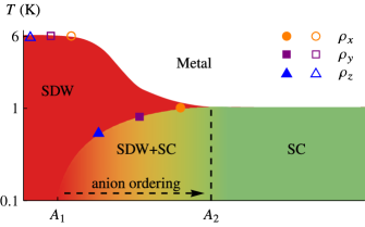
Figure 1: Phase diagram of SDW in (TMTSF)₂ClO₄ recreated from resistivity data in Ref. [25].

In (TMTSF)₂ClO₄ there is an additional degree of freedom and driving parameter. The ClO₄ anions, which lack the inversion symmetry and possess an electric dipole moment, order below the transition temperature $T_{\text{AO}}=24$ K $>T_{\text{cDW}}$ with wave vector $\bm{Q}_{\text{AO}}=(0,1/2,0)$ [15, 16]. This anion ordering (AO) doubles the lattice along the $y$-axis and splits the FS in four open sheets (see, e.g., Fig. 1b of Ref. [24] or Fig. 3b and 5b of Ref. [45]). The latter deteriorates FS nesting and suppresses DW [16, 46, 47, 45, 48], giving rise to superconductivity [16, 24, 25, 26, 49].

The electron dispersion in (TMTSF)₂ClO₄ in the anion-ordered phase in the new folded Brilluin zone can also be approximately described by Eq. (1) with two branches, splitted by $2\Delta_{\text{AO}}$ (see Appendix A):

$$t_{\perp}(\bm{k}_{\perp})\simeq\pm\left[\Delta_{\text{AO}}+2t_{b}^{\prime}\cos(2k_{y}b)\right].$$ (4)

This dispersion results to the antinesting term given by Eq. (30), which controls the SDW phase diagram in (TMTSF)₂ClO₄.

The anion ordering can be controlled by the cooling rate near $T_{\text{AO}}=24$ K. In rapidly cooled (quenched) samples the anions remain disordered, and the DW is not suppressed, while SC does not appear. The slowly cooled (relaxed) samples have $\Delta_{\text{AO}}\approx 14$ meV [45, 49], which destroys the SDW and leads to a homogeneous superconductivity. Hence, the cooling rate in (TMTSF)₂ClO₄ enables to reveal a rich phase diagram even at ambient pressure, where DW phase is favored for strong disorders (rapid cooling), SC and DW coexist at intermediate, and a uniform SC sets in for weak disorders (slow cooling). The phase diagram in (TMTSF)₂ClO₄ is qualitatively similar to that in (TMTSF)₂PF₆ with the replacement of pressure by anion ordering, as illustrated in Fig. 1.

An external magnetic field $B$ via the Zeeman splitting energy $\Delta_{\text{Z}}=\mu_{B}gB$ shifts in opposite directions the FS for different spin projections, which damps CDW but not SDW. The magnetic field also affects the orbital electron motion, which leads to the beautiful effect of field-induced spin-density wave [15, 16], to the quantized nesting and the complicated phase diagram. However, if the magnetic field is directed along the conducting layers, its orbital effect is weak, and the new dispersion is given by

$$t_{\perp}({\bm{k}}_{\perp})\simeq-2t_{b}\cos(k_{y}b)-2t_{b}^{\prime}\cos(2k_{y}b)\pm\Delta_{\text{Z}}.$$ (5)

This results to the same antinesting term (30) as for AO, with the replacement $\Delta_{\text{AO}}\to\Delta_{\text{Z}}$. The CDW phase diagram in a magnetic field acting only by the Zeeman splitting is already quite interesting and complicated [50].

III Mean field approach and Landau expansion for the density wave

III.1 Bogoliubov transformation

The electron Hamiltonian consist of the free electron part $H_{0}$ and the interaction part $H_{\text{int}}$:

$$\begin{split}&H=H_{0}+H_{\text{int}},\\ &H_{0}=\sum_{\bm{k}}\varepsilon(\bm{k})a_{\bm{k}}^{\dagger}a_{\bm{k}},\\ &H_{\text{int}}\ =\frac{1}{2}\sum_{\bm{k}\bm{k}^{\prime}\bm{Q}}V_{\bm{Q}}a_{\bm{k}+\bm{Q}}^{\dagger}a_{\bm{k}}a_{\bm{k}^{\prime}-\bm{Q}}^{\dagger}a_{\bm{k}^{\prime}}.\end{split}$$ (6)

We consider the interactions at the wave vector $\bm{Q}$ close to the nesting vector $\bm{Q}=(\pm 2k_{F},\pi/b,\pi/c)$. If the deviations from $\bm{Q}_{0}$ are small, we can approximate the interaction function as $V(\bm{Q})\approx V(\bm{Q}_{0})=U$. Next, in the mean-field approximation we introduce the order parameter

$$\Delta_{\bm{Q}}=U\sum_{\bm{k}}\langle a_{\bm{k}-{\bm{Q}}}^{\dagger}a_{\bm{k}}\rangle_{T}=U\sum_{\bm{k}}\frac{\operatorname{Tr}\left(a^{\dagger}_{\bm{k}-\bm{Q}}a_{\bm{k}}e^{-\beta H}\right)}{Z}.$$ (7)

We now set $\Delta_{\bm{k}}=\Delta\delta_{\bm{k},\pm\bm{Q}}$, where $\bm{Q}=(2k_{F},\pi/b,0)+\bm{q}$ with $|\bm{q}|\ll k_{F}$. The resulting mean–field Hamiltonian

$$H_{\text{MF}}=\sum_{\bm{k}}\varepsilon(\bm{k})a_{\bm{k}}^{\dagger}a_{\bm{k}}+\sum_{\bm{k}}\Delta a_{\bm{k}+\bm{Q}}^{\dagger}a_{\bm{k}}-\frac{\Delta^{2}}{2U}.$$ (8)

can be diagonalized via Bogoliubov transformation. In order to do so we rewrite the Hamiltonian in a matrix form as

$$\begin{split}&H_{\text{MF}}=\sum_{\bm{k}}\psi^{\dagger}_{\bm{k}}h_{\bm{k}}\psi_{\bm{k}}-\frac{\Delta^{2}}{2U},\\ &h=\begin{pmatrix}\varepsilon(\bm{k})&\Delta\\ \Delta&\varepsilon(\bm{k}+\bm{Q})\end{pmatrix},\\ &\psi^{\dagger}(\bm{k})=\begin{pmatrix}a^{\dagger}_{\bm{k}}&a^{\dagger}_{\bm{k}+\bm{Q}}\end{pmatrix}.\end{split}$$ (9)

The spectrum of the Hamiltonian is then given by the eigenvalues $E_{\pm}(\bm{k})$ of the matrix $h$ which are

$$E_{\pm}(\bm{k})=\varepsilon_{+}(\bm{k})\pm\sqrt{\varepsilon_{-}^{2}(\bm{k})+\Delta^{2}},$$ (10)

where

$$\varepsilon_{\pm}(\bm{k})\equiv\frac{\varepsilon(\bm{k})\pm\varepsilon(\bm{k}+\bm{Q})}{2}.$$ (11)

The operators $\gamma_{\bm{k}}$, $\mu_{\bm{k}}$ in which the Hamiltonian is diagonal are defined by the eigenvectors of $h$. They are obtained by a unitary transformation

$$\begin{pmatrix}\gamma_{\bm{k}}\\ \mu_{\bm{k}}\end{pmatrix}=\begin{pmatrix}u&v\\ -v&u\end{pmatrix}\begin{pmatrix}a_{\bm{k}}\\ a_{\bm{k}+\bm{Q}}\end{pmatrix}$$ (12)

such that $u^{2}+v^{2}=1$ and $\Delta(u^{2}-v^{2})+2uv\varepsilon_{-}(\bm{k})=0$. Finally the diagonalized Hamiltonian is

$$\begin{split}H&=\sum_{\bm{k}}\left(E_{+}(\bm{k})\gamma^{\dagger}_{\bm{k}}\gamma_{\bm{k}}+E_{-}(\bm{k})\mu^{\dagger}_{\bm{k}}\mu_{\bm{k}}\right)\\ &-\frac{1}{2}\sum_{\bm{k}}\left(E_{+}(\bm{k})-E_{-}(\bm{k})\right)-\frac{\Delta^{2}}{2U}.\end{split}$$ (13)

Now given that the Hamiltonian is diagonal in fermionic operators $\gamma_{\bm{k}}$, $\mu_{\bm{k}}$ and there are only four states $|n_{\gamma}n_{\mu}\rangle=\{|00\rangle,|01\rangle,|10\rangle,|11\rangle\}$, the partition function $Z=\operatorname{Tr}\exp\{-H\mathrm{{}_{\text{MF}}}/T\}$ can be easily calculated:

$$\begin{split}Z&=e^{-\Delta^{2}/2U}\prod_{\bm{k}}e^{(E_{+}+E_{-})/2T}\times\\ &\times\operatorname{Tr}\begin{pmatrix}1&0&0&0\\ 0&e^{-E_{+}/T}&0&0\\ 0&0&e^{-E_{-}/T}&0\\ 0&0&0&e^{-(E_{+}+E_{-})/T}\end{pmatrix}=\\ &=e^{-\Delta^{2}/2U}\prod_{\bm{k}}4\cosh\frac{E_{+}(\bm{k})}{2T}\cosh\frac{E_{-}(\bm{k})}{2T}.\end{split}$$ (14)

And the free energy $F=-T\ln Z$ is

$$F=-T\sum_{\bm{k}}\ln\left(4\cosh\frac{E_{+}(\bm{k})}{2T}\cosh\frac{E_{-}(\bm{k})}{2T}\right)-\frac{\Delta^{2}}{2U}.$$ (15)

III.2 Free energy expansion

We are interested in the Landau–Ginzburg expansion coefficients of the free energy in powers of $\Delta$:

$$F\simeq\frac{A}{2}\Delta^{2}+\frac{B}{4}\Delta^{4}+\ldots$$ (16)

By differentiating this expression one obtains

$$\frac{\partial F}{\partial\Delta}\simeq A\Delta+B\Delta^{3}+\ldots$$ (17)

This means that the free energy expansion coefficients can be calculated by expanding into the Taylor series not the free energy itself, but the function

$$\begin{split}&F^{\prime}=\frac{\partial F}{\partial\Delta}=-\frac{\Delta}{2\sqrt{\varepsilon_{-}^{2}(\bm{k})+\Delta^{2}}}\times\\ &\times\sum_{\bm{k}}\left(\tanh\dfrac{E_{+}(\bm{k})}{2T}-\tanh\dfrac{E_{-}(\bm{k})}{2T}\right)-\frac{\Delta}{U}.\end{split}$$ (18)

Next we use the following relation to represent the hyperbolic tangents as a sum over odd Matsubara frequencies $\omega=\pi T(2n+1)$:

$$\frac{1}{4\alpha}\left\{\tanh\frac{\alpha-\beta}{2T}+\tanh\frac{\alpha+\beta}{2T}\right\}=T\sum_{\omega}\frac{1}{(\omega+i\beta)^{2}+\alpha^{2}}.$$ (19)

Substituting $\alpha=\sqrt{\varepsilon_{-}^{2}({\bm{k}})+\Delta^{2}}$ and $\beta=\varepsilon_{+}({\bm{k}})$ we find

$$\begin{split}&T\sum_{\omega}\frac{1}{(\omega+i\varepsilon_{+}({\bm{k}}))^{2}+\varepsilon_{-}^{2}({\bm{k}})+\Delta^{2}}=\\ &=\frac{\tanh\dfrac{E_{+}({\bm{k}})}{2T}-\tanh\dfrac{E_{-}({\bm{k}})}{2T}}{4\sqrt{\varepsilon_{-}^{2}({\bm{k}})+\Delta^{2}}}.\end{split}$$ (20)

Finally, substituting this equality in (18) we end up with the function which expansion coefficients we will study further:

$$\begin{split}F^{\prime}&=-2T\sum_{{\bm{k}}\omega}\frac{\Delta}{(\omega+i\varepsilon_{+}({\bm{k}}))^{2}+\varepsilon_{-}^{2}({\bm{k}})+\Delta^{2}}-\frac{\Delta}{U}\simeq\\ &\simeq A\Delta+B\Delta^{3}+\dots\end{split}$$ (21)

As it follows from eqs. (16) – (17), the expansion coefficient of the free–energy $F$ at $\Delta^{n}$ is obtained by dividing by $n$ the coefficient of the expansion of $F^{\prime}$. For the first two coefficients we obtain

$$A=-2T\sum_{{\bm{k}}\omega}\frac{1}{[\omega+i\varepsilon_{+}({\bm{k}})]^{2}+\varepsilon_{-}^{2}({\bm{k}})}-\frac{1}{U}$$ (22)

and

$$B=2T\sum_{{\bm{k}}\omega}\frac{1}{\left[(\omega+i\varepsilon_{+}({\bm{k}}))^{2}+\varepsilon_{-}^{2}({\bm{k}})\right]^{2}}.$$ (23)

If $B>0$, the DW-metal phase transition is of the second order, and only the first two coefficients $A$ and $B$ are sufficient for its description. If $B<0$, the phase transition may be of the first order, and next coefficients $C$ and even $D$ if $C\leq 0$ are required for its description.

The sum over $\bm{k}$ in Eq. (21) for macroscopic sample is equivalent to the integral

$$\sum_{\bm{k}}=2\int\frac{\mathop{}\!\mathrm{d}k_{x}}{2\pi}\int_{-\pi/b}^{\pi/b}\frac{\mathop{}\!\mathrm{d}k_{y}}{2\pi}.$$ (24)

The factor $2$ appears because of two Fermi-surface sheets at $k_{x}\approx\pm k_{F}$. Usually, for simplicity the integration limits over $k_{x}$ in Eq. (24) are taken to be infinite: $k_{x}\in\left[-\infty,\infty\right]$, and the resulting logarithmic divergence of the coefficient $A$ is regularized by the definition of the transition temperature $T_{c}$ (see Appendix B). However, in this case for the dispersion in Eqs. (1) and (2) all the coefficients $A,B,C,D$ vanish at the same point at $T=0$ and $t_{b}^{\prime}=t_{b}^{\prime\ast}$, which does not allow one to determine the type of this phase transition. Hence, below we consider both infinite and finite integration limits as well as the case beyond the linear approximation when the spectrum in $k_{x}$ direction is $\propto\cos(k_{x}a)$.

IV Calculation of the Landau expansion coefficients for the density wave and its phase diagram in quasi-1D metals

In this section we take the quasi-1D electron (1) linearised in the $k_{x}$ direction, and explicitly calculate the first coefficients of the Landau expansion for the DW free energy given by Eqs. (21)-(23). This helps us to analyze the type of DW-metal phase transition in organic metals.

IV.1 Infinite limits of integration over $k_{x}$

The integration of Eq. (21) over $k_{x}$ in infinite limits for the linearized electron dispersion (1) gives the well-known result for the DW free energy:

$$F^{\prime}=-\frac{4\pi T}{\hbar v_{F}}\sum_{\omega}\left\langle\frac{\Delta}{\sqrt{(\omega+i\varepsilon_{+}(k_{y}))^{2}+|\Delta|^{2}}}\right\rangle_{k_{y}}-\frac{\Delta}{U}.$$ (25)

The free energy expansion coefficients are obtained by expanding the r.h.s. of this equation over $|\Delta|^{2}$:

$$F^{\prime}\simeq-\frac{4\pi T}{\hbar v_{F}}\sum_{\omega}\left\langle\frac{\Delta\operatorname{sgn}\omega}{\omega+i\varepsilon_{+}(\bm{k})}-\frac{\Delta^{3}\operatorname{sgn}\omega}{2(\omega+i\varepsilon_{+}(\bm{k}))^{3}}\right\rangle_{k_{y}}-\frac{\Delta}{U}.$$ (26)

The coefficient at the linear term

$$A_{\infty}=-\frac{4\pi T}{\hbar v_{F}}\sum_{\omega}\left\langle\frac{\operatorname{sgn}\omega}{\omega+i\varepsilon_{+}(\bm{k})}\right\rangle_{k_{y}}-\frac{1}{U}$$ (27)

is divergent when sum over $\omega$ is taken. The divergence is regularized by introducing the critical temperature $T_{c0}$ at which the DW phase transition occurs when $t^{\prime}_{b}=0$, see Appendix B. As a results we obtain

$$A_{\infty}=-\frac{4}{\hbar v_{F}}\left[\ln\frac{T_{c0}}{T}+\psi\left(\frac{1}{2}\right)-\left\langle\operatorname{Re}\psi\left(\frac{1}{2}+\frac{i\varepsilon_{+}(\bm{k})}{2\pi T}\right)\right\rangle_{k_{y}}\right],$$ (28)

where $\psi(x)=\mathop{}\!\mathrm{d}/\mathop{}\!\mathrm{d}x\ln\Gamma(x)$ is the digamma function.

The type of the phase transition is defined by the coefficient in front of the $\sim\Delta^{3}$ term in the expansion. This coefficient is

$$\begin{split}B_{\infty}&=\frac{2\pi T}{\hbar v_{F}}\sum_{\omega}\left\langle\frac{\operatorname{sgn}\omega}{(\omega+i\varepsilon_{+}(\bm{k}))^{3}}\right\rangle_{k_{y}}\\ &=-\frac{1}{4\pi^{2}T^{2}\hbar v_{F}}\left\langle\operatorname{Re}\psi^{\prime\prime}\left(\frac{1}{2}+\frac{i\varepsilon_{+}(\bm{k})}{2\pi T}\right)\right\rangle_{k_{y}}.\end{split}$$ (29)

The self-consistency equation (SCE) for the order parameter $\Delta$ is obtained from the condition $F^{\prime}=0$ for the minimum of free energy. This SCE for the DW state, even in the presence of both spin and charge coupling constants and in a magnetic field, was derived previously [50] using the equations for the Green’s function. The analytical expression for free energy $F$ up to a constant factor can be obtained from the integration of these SCE over $\Delta$, and the missing coefficient can be obtained from the comparison of Eq. (25) above with the Eq. (22) of Ref. [50]. The comparison of Eqs. (28) and (29) above with Eqs. (24),(31) and (32) of Ref. [50] gives the relations $A_{\infty}=(K_{\sigma}^{(1)}-1)(4\pi/U)$ and $B_{\infty}=K_{\sigma}^{(3)}4\pi/U$ between the functions $K_{\sigma}^{(1)}$ and $K_{\sigma}^{(3)}$ derived in Ref. [50].

The phase transition changes its order from second to first when the coefficient $B$ becomes negative. The function (29) generally decreases as the parameter $\left|\varepsilon_{+}\right|$ grows, but this decrease depends on the details of $\left|\varepsilon_{+}\right|$, in particular, on the ratio $\Delta_{\text{AO}}/t_{b}^{\prime}$. Below we analyze the dependence $B(\varepsilon_{+})$ on the DW-metal transition line and the type of this phase transition in quasi-1D organic superconductors.

IV.2 Application to organic metals

Figure 2: Calculated transition lines as a function of (a) anion ordering gap $\Delta_{\text{AO}}$ for specific $t_{b}^{\prime}$: $t_{b}^{\prime}=0$ (solid blue line), $2t_{b}^{\prime}=\Delta_{0}/2$ (dashed red line), $2t_{b}^{\prime}=0.75~{}\Delta_{0}$ (dotted green line), $2t_{b}^{\prime}=0.9~{}\Delta_{0}$ (magenta dash-dotted line), and $2t_{b}^{\prime}=0.99~{}\Delta_{0}$ (long-dashed orange line); (b) $t_{b}^{\prime}$ for specific anion ordering gap $\Delta_{\text{AO}}$: $\Delta_{\text{AO}}=0$ (solid blue line), $\Delta_{\text{AO}}=T_{c0}/2$ (dashed red line), $\Delta_{\text{AO}}=0.8~{}T_{c0}$ (dotted green line), $\Delta_{\text{AO}}=0.98~{}T_{c0}$ (dash-dotted magenta line), $\Delta_{\text{AO}}=1.09~{}T_{c0}$ (long-dashed brown line), $\Delta_{\text{AO}}=1.15~{}T_{c0}$ (thin dashed orange line) and $\Delta_{\text{AO}}=1.3~{}T_{c0}$ (solid thin black line). $T_{c}\left(\Delta_{\text{AO}}\right)$ is determined from the condition $A_{\infty}=0$ and Eqs. (28) and (30). The crosses on each line approximately indicate the points where the DW-metal phase transition changes its type from second to first. This phase diagram is qualitatively applicable to (TMTSF)₂ClO₄ and also to (TMTSF)₂PF₆ at $\Delta_{\text{AO}}=0$.

From Eqs. (4) and (11) we obtain the antinesting term in (TMTSF)₂ClO₄:

$$\varepsilon_{+}({\bm{k}})=-2t_{b}^{\prime}\cos(2k_{y}b)+\Delta_{\text{AO}}.$$ (30)

This antinesting term also describes (TMTSF)₂PF₆ as a limiting case $\Delta_{\text{AO}}=0$.

In the case of band-splitted electron dispersion, as in Eqs. (4) for AO or (5) for Zeeman splitting, for each band $\eta^{\prime}=\pm 1$ the sum over $\bm{k}$ in Eqs. (6)-(24) also contains the sum over two bands $\eta=\pm 1$: $\sum_{\bm{k}}\to\sum_{\bm{k},\eta}$. In this sum only one of two terms, corresponding to $\eta^{\prime}\neq\eta$, contains the antinesting term (30). The other perfect-nesting term, corresponding to $\eta^{\prime}=\eta$, adds a constant term (45) to the coefficient $A$. It renormalizes the transition temperature $T_{c0}$, but does not change Eq. (28) and the transition lines normalized to $T_{c0}$ and shown in Fig. 2. For different bands $\eta^{\prime}=\pm 1$ the antinesting term has opposite sign, therefore the DW wave vector does not shift along $k_{x}$ for not very large band splitting (see Ref. [50] for the phase diagram at $t_{b}^{\prime}=0$). Since the digamma function $\psi\left(1/2+i\,x\right)$ is symmetric to $x\to-x$, both bands $\eta^{\prime}=\pm 1$ are described by the same formulas.

The DW-metal transition line $T_{c}(\Delta_{\text{AO}},t_{b}^{\prime})$, given by equation $A_{\infty}=0$ and shown in Fig. 2, suggests several interesting observations. Both $t_{b}^{\prime}$ and $\Delta_{\text{AO}}$ suppress $T_{c}$, as expected. However, the increase of $t_{b}^{\prime}$ increases the critical value of $\Delta_{\text{AO}}^{\ast}$ of the DW-metal phase transition. This counterintuitive observation can be shown analytically. In the limit of zero temperature, one can obtain an exact expression for $\Delta_{\text{AO}}^{\ast}(t_{b}^{\prime})$. Using the asymptotic approximation for digamma function $\operatorname{Re}\psi\left(1/2+ix\right)\simeq\ln x-1/(24x^{2})$ at $x\gg 1$ and substituting Eq. (28) to $A_{\infty}=0$, we get the equation for transition point

$$\left\langle\ln\left(\varepsilon_{+}\right)\right\rangle_{k_{y}}=\ln(2\pi T_{c0})+\psi(1/2).$$ (31)

Substituting Eq. (30) and performing the integration over $k_{y}$ we obtain the solution to this equation, valid at $\Delta_{\text{AO}}\leq 2t_{b}^{\prime}$:

$$\frac{\Delta_{\text{AO}}^{\ast}}{T_{c0}}=2\pi e^{\psi(1/2)}+\frac{t_{b}^{\prime 2}/T_{c0}^{2}}{2\pi e^{\psi(1/2)}}.$$ (32)

In the limit $t_{b}^{\prime}=0$ we obtain $\Delta_{\text{AO}}/T_{c0}=2\pi e^{\psi(1/2)}\approx 0.88$ (the intersection of the blue line with the $t_{b}^{\prime}$-axis in Fig. 2a). The maximal value of $\Delta_{\text{AO}}^{\ast}\left(t_{b}^{\prime}\right)$ is at $2t_{b}^{\prime}=\Delta_{\text{AO}}^{\ast}=2t_{b}^{\prime\ast}$:

$$\text{max}\left\{\Delta_{\text{AO}}^{\ast}\right\}=2t_{b}^{\prime\ast}=4\pi e^{\psi(1/2)}T_{c0}\approx 1.764\,T_{c0}.$$ (33)

In contrast to $\Delta_{\text{AO}}^{\ast}\left(t_{b}^{\prime}\right)$, within our model $t_{b}^{\prime\ast}$ is independent of $\Delta_{\text{AO}}$ as long as $\Delta_{\text{AO}}<\Delta_{\text{AO}}^{\ast}(t_{b}^{\prime})$. This is illustrated in Fig. 2b, where all transition lines cross at $t_{b}^{\prime}=t_{b}^{\prime\ast}$ at $T=0$.

The second our result obtained for the antinesting term in Eq. (30) is the dependence of $B_{\infty}$, given by Eq. (29), on the parameters $\Delta_{\text{AO}}$ and $t_{b}^{\prime}$. The point $B_{\infty}=0$ on the $T_{c}(\Delta_{\text{AO}},t_{b}^{\prime})$ transition line, where this phase transition changes from the second to first order, is indicated by crosses in Fig. 2. From Fig. 2a we see that at any $t_{b}^{\prime}<t_{b}^{\prime\ast}$ there is a critical value $\Delta_{\text{AO}}^{\rm{o}}$ of $\Delta_{\text{AO}}^{\ast}(t_{b}^{\prime})$ such that at $\Delta_{\text{AO}}>\Delta_{\text{AO}}^{\rm{o}}$ there is a finite temperature interval $0<T_{c}<T_{c}^{\rm{o}}$, where $B_{\infty}<0$ and the DW-metal phase transition is of the first order.

In contrast to this, the increase of $t_{b}^{\prime}$ on the interval $0<t_{b}^{\prime}<t_{b}^{\prime\ast}$ at fixed $\Delta_{\text{AO}}<\Delta_{\text{AO}}^{\rm{o}}$ does not leads to the sign change of $B_{\infty}$, given by Eqs. (29) and (30). This is illustrated in Fig. 2b by the absence of crosses on the transition lines at $\Delta_{\text{AO}}<T_{c0}$. The dependence $B_{\infty}(t_{b}^{\prime})$ at $\Delta_{\text{AO}}=0$ and $T\approx 0.6T_{c0}$ is shown by the dashed green line in Fig. 3. This line crosses the abscissa axis at $t_{b}^{\prime}>t_{b}^{\prime\ast}$, and $B_{\infty}(t_{b}^{\prime})>0$ on the entire interval $0<t_{b}^{\prime}<t_{b}^{\prime\ast}$, which means the second-order DW-metal phase transition at any $t_{b}^{\prime}$.

At $\Delta_{\text{AO}}=0$ $B_{\infty}=0$ only at $t_{b}^{\prime}=t_{b}^{\prime\ast}$ and $T=0$, i.e. the interval $0<T_{c}<T_{c}^{\rm{o}}$ of the first-order phase transition is formally zero. The point $t_{b}^{\prime}=t_{b}^{\prime\ast}$ and $T=0$ is very special: at this point not only $A_{\infty}=0$ and $B_{\infty}=0$, but also next coefficients of the Landau expansion vanish: $C_{\infty}=0$ and $D_{\infty}=0$. This degeneracy is a consequence of our oversimplified model, where we took the dispersion given by Eqs. (1),(2),(30) and the Fermi energy $E_{F}$ and the band width infinitely large, $\gg t_{b}^{\prime},\Delta_{\text{AO}}$. This degeneracy is lifted, for example, if one takes finite limits of integration over $k_{x}$, corresponding to a finite band width and Fermi energy, as described in the next subsection IV.3. A more realistic electron dispersion also gives a finite interval of the first-order DW-metal phase transition, as shown below in subsections IV.4 and IV.5.

IV.3 Finite limits of integration over $k_{x}$

Let us now take $\Delta_{\text{AO}}=0$ and consider finite limits of integration $k_{x}\in\left[-K,K\right]$. Then equation (25) becomes

$$F^{\prime}=-\frac{4\pi T}{\hbar v_{F}}\sum_{\omega}\left\langle\frac{\Delta\,f(\Delta)}{\sqrt{(\omega+i\varepsilon_{+}(\bm{k}))^{2}+|\Delta|^{2}}}\right\rangle_{k_{y}}.$$ (34)

The additional factor $f(\Delta)$ is

$$\begin{split}f(\Delta)&=\frac{1}{\pi}\left(\arctan\frac{v_{F}(K+k_{F})-2t_{b}\cos(2k_{y})}{\sqrt{(\omega+i\varepsilon_{+}(\bm{k}))^{2}+\Delta^{2}}}+\right.\\ &+\left.\arctan\frac{v_{F}(K-k_{F})-2t_{b}\cos(2k_{y})}{\sqrt{(\omega+i\varepsilon_{+}(\bm{k}))^{2}+\Delta^{2}}}\right).\end{split}$$ (35)

We expand the r.h.s of (34) up to third order in $\Delta$:

$$\begin{split}&\Delta\simeq-\frac{4\pi T}{\hbar v_{F}}\sum_{\omega}\left\langle\frac{f(0)\operatorname{sgn}\omega}{\omega+i\varepsilon_{+}(\bm{k})}\Delta+\right.\\ &+\left.\frac{1}{2}\left[\frac{f^{\prime\prime}(0)\operatorname{sgn}\omega}{\omega+i\varepsilon_{+}(\bm{k})}-\frac{f(0)\operatorname{sgn}\omega}{(\omega+i\varepsilon_{+}(\bm{k}))^{3}}\right]\Delta^{3}\right\rangle_{k_{y}}.\end{split}$$ (36)

The coefficient at the linear term is

$$A_{K}=-\frac{4\pi T}{\hbar v_{F}}\sum_{\omega}\left\langle\frac{f(0)\operatorname{sgn}\omega}{\omega+i\varepsilon_{+}(\bm{k})}\right\rangle_{k_{y}}-\frac{1}{U}.$$ (37)

Due to finiteness of the limits of integration it is not divergent any more.

The coefficient at the qubic term is

$$B_{K}=\frac{2\pi T}{\hbar v_{F}}\sum_{\omega}\left\langle\frac{f(0)\operatorname{sgn}\omega}{(\omega+i\varepsilon_{+}(\bm{k}))^{3}}-\frac{f^{\prime\prime}(0)\operatorname{sgn}\omega}{\omega+i\varepsilon_{+}(\bm{k})}\right\rangle_{k_{y}}.$$ (38)

Numerically calculating the sum and the integral in Eq. (38) we confirm that $B_{K}$ at finite $K$ and low enough $T$ changes its sign at $t^{\prime}_{b}<t^{\prime\ast}_{b}$. Hence, the finite limits of integration change the order of DW-metal phase transition from second to first one. The corresponding plot is presented in Fig. 3, the limits of integration are chosen as $K=\pi/b$. The solid blue line $B_{K}(t^{\prime}_{b})$ even at rather large temperature $T=0.6T_{c0}$ crosses the abscissa axis at $t^{\prime\rm{o}}_{b}<t^{\prime\ast}_{b}$, which indicates a large temperature interval of the first-order DW-metal phase transition. This results predicts a finite temperature $0<T_{c}<T_{c}^{\rm{o}}$ and pressure interval of the first-order SDW-metal phase transition in (TMTSF)₂PF₆.

Figure 3: Plots of expansion coefficients $B_{K}$ (solid blue line) and $B_{\infty}$ (dashed green line) as functions of $t_{b}^{\prime}$ at $T=0.6~{}T_{c0}$. The vertical axis scale is in units $4\pi T_{c0}/\hbar v_{F}$, where $T_{c0}$ is the critical temperature at $t^{\prime}_{b}=0$, see Appendix B. The horizontal scale is in units $t_{b}^{\prime*}$ – the value of $t_{b}^{\prime}$ at which the DW-phase is destroyed, i.e. $A_{K}=0$. The inset shows similar plot for the next expansion coefficient $C$ at $\Delta^{6}$.

IV.4 Influence of fourth harmonic in quasi-1D electron dispersion on the DW phase diagram

The electron spectrum given by Eq. (2) is oversimplified. Since all odd harmonics of the $k_{y}$ electron dispersion do not violate the FS nesting in our model, the simplest modification of electron dispersion in Eq. (2) affecting the phase diagram is adding the fourth harmonics. When the limits of integration over $k_{x}$ are kept infinite but the fourth harmonic $4t^{\prime\prime}_{b}\cos(4k_{y}b)$ is introduced to the spectrum the formal expression (29) for the coefficient $B$ holds, but the energy $\varepsilon_{+}(\bm{k})$ becomes

$$\varepsilon_{+}(\bm{k})=-2t^{\prime}_{b}\cos(2k_{y}b)-2t^{\prime\prime}_{b}\cos(4k_{y}b).$$ (39)

This additional term reduces the coefficient $B$ and leads to dependence $B(t^{\prime}_{b})$ similar to $B_{K}(t^{\prime}_{b})$ (presented by solid line in Fig. 3), i.e. when the limits of integration are finite. Hence, taking a more realistic electron spectrum by adding higher harmonics to Eq. (2) lifts the above mentioned degeneracy $A=B=0$ at $t^{\prime}_{b}=t^{\prime\ast}_{b}$ and $T=0$ even for infinite integration limits $K=\infty$. The fourth harmonic in quasi-1D electron dispersion decreases the coefficient $B$ of the Landau expansion for free energy and favors the first order of DW-metal phase transition.

IV.5 Nonlinearised spectrum

We now discard the linear approximation of the spectrum in the $k_{x}$ direction, i.e. replace the spectrum (1) with

$$\varepsilon(\bm{k})=-2t_{a}\cos(k_{x}a)+t_{\perp}(\bm{k}_{\perp}).$$ (40)

In this case the analytical integration with respect to $k_{x}$ of (21) is not possible. Also the integration limits are required to be finite: $k_{x}\in[-\pi/a,\pi/a]$.

Accordingly we expand the r.h.s. of equation (21) in powers of $\Delta$:

$$\begin{split}F^{\prime}&\simeq-2T\sum_{\bm{k}\omega}\left(\frac{\Delta}{(\omega+i\varepsilon_{+}(\bm{k}))^{2}+\varepsilon_{-}(\bm{k})}\right.-\\ &\left.-\frac{\Delta^{3}}{[(\omega+i\varepsilon_{+}(\bm{k}))^{2}+\varepsilon_{-}(\bm{k})]^{2}}\right)-\frac{\Delta}{U}.\end{split}$$ (41)

Once again performing numerical integration over $k_{x}$, $k_{y}$ and summation over $\omega$ we confirm that the coefficient $B$ at $\Delta^{3}$ changes sign as function of $t_{b}^{\prime}$ at $t_{b}^{\prime}<t_{b}^{\prime\ast}$. Thus we conclude that the first order phase transition emerges also when the linear approximation of electron spectrum along $k_{x}$ is not made.

V Discussion and conclusion

Our calculations show that a DW-metal transition, driven by an external parameter which deteriorates the FS nesting, typically goes by first order at low enough temperature. When such a driving parameter splits the energy spectrum and the Fermi surfaces, as in the case of anion ordering in (TMTSF)₂ClO₄ or of magnetic field acting via Zeeman splitting on a CDW, as described in Sec. IIB, the temperature interval of the first-order phase transition is rather wide, $\sim T_{c0}/2$ (see Fig. 2a). This explains the spatial phase segregation and coexistence of SDW-metal or SDW-SC phases observed in (TMTSF)₂ClO₄. When such a driving parameter is pressure and the antinesting term in electron dispersion, as described by the amplitude $t_{b}^{\prime}$ of the second harmonic in Eq. (2), this interval is smaller and appears only when one goes beyond the simplest model by taking into account the finite bandwidth and Fermi energy (see Sec. IV.3 and Fig. 3) or/and more realistic electron dispersion (see Secs. IV.4 and IV.5).

The model electron dispersions used in our calculations and given by Eqs. (1),(2),(4),(30),(39),(40) still differ from actual electron spectrum in organic metals (TMTSF)₂PF₆ and (TMTSF)₂ClO₄, e.g., calculated using DFT in Refs. [45, 51, 48]. The main difference comes from low triclinic crystal symmetry and higher harmonics of electron dispersion. Nevertheless, the result obtained about the negative coefficient $B$ of the Landau expansion for DW free energy and of the first-order phase transition between DW and metallic state at low $T$ are rather robust to small variations of electron dispersion and should survive also for more realistic electron spectrum.

The obtained first order of DW-metal phase transition explains the spatial segregation of SDW and SC/metal phases observed in (TMTSF)₂PF₆ and (TMTSF)₂ClO₄, or of CDW and SC/metal phases in $\upalpha$-(BEDT-TTF)₂KHg(SCN)₄, resulting to DW coexistence with superconductivity. The parameters and properties of phase nucleation during the first-order phase transition was extensively studied in various systems [52, 53]. Nevertheless, a quantitative application of this theory to the particular DW–metal/SC phase transitions is still missing.

The phase segregation during the first-order DW-metal phase transition happens on a rather large length scale $\gtrsim 1$ µm, which explains the observation of angular magnetoresistance oscillations (AMRO) in (TMTSF)₂PF₆ [20] and in (TMTSF)₂ClO₄ [24], i.e. the oscillating dependence of interlayer magnetoresistance on the tilt angle of magnetic field $\bm{B}$ [29]. The latter is possible only if the size of metallic islands along $x$-axis exceeds the so-called quasi-1D magnetic length $l_{B}=\hbar/eBb\sim 1$ µm [29, 20]. In addition, the field-induced SDW (FISDW) [15, 16], i.e. the oscillating dependence of the SDW transition temperature on the strength $B$ of magnetic field, are also observed in (TMTSF)₂PF₆ [20] and in (TMTSF)₂ClO₄ [24], which is also possible only if the size of metal islands in SDW matrix exceeds $l_{B}=\hbar/eBb\sim 1$ µm. Other microscopic theories, including superconductivity inside soliton walls of DW order parameter [19, 35, 33], cannot explain such a large size of metal/SC domains, and, hence, contradict the AMRO and FISDW experiments [20, 24]. Note that our scenario of DW-SC phase separation is also consistent with the severalfold enhancement of the upper critical field $H_{c2}$ observed in the coexistence phase of these organic superconductors [17, 27], because the SC domain size $\sim 1$ µm is comparable to the magnetic penetration depth $\lambda$, which enhances $H_{c2}$ [36]. In (TMTSF)₂ClO₄ the in-plane penetration depth is rather large [54], $\lambda_{ab}(T=0)\approx 0.86$ µm, and increases even more at $T\to T_{\text{cSC}}$. Similarly large value of $\lambda$ is expected in (TMTSF)₂PF₆ and $\upalpha$-(BEDT-TTF)₂KHg(SCN)₄.

In organic metals the DW phase transition temperature $T_{\text{cDW}}$ is usually much higher than the SC transition temperature $T_{\text{cSC}}$. This is a general situation, which happens in many other compounds where CDW or SDW coexists with superconductivity [3, 4]. This difference of $T_{\text{cDW}}$ and $T_{\text{cSC}}$ appears because for the formation of a DW the usually strong repulsive Coulomb e-e interaction is suitable, while for the Cooper pairing only the e-e attraction via phonons or via other mediating quasi-particle is needed, which usually competes with the strong Coulomb repulsion. Therefore, in our analysis we disregarded the influence of superconductivity on DW phase diagram. Similar approximation to study the spatial inhomogeneity of SDW phase and the properties of superconductivity on a DW background was used in Refs. [35, 30, 34, 33]. However, when the DW is almost destroyed by the antinesting parameter, so that $T_{\text{cDW}}\sim T_{\text{cSC}}$, the SC may influence the DW. This mutual influence of SDW and SC can be analyzed by studying two order parameters simultaneously [55, 56, 57], but its realization for a more complicated DW phase diagram and the antinesting term in electron dispersion is still missing. By analogy with a simpler case [56], this interplay is expected to reduce the DW region on the phase diagram and to favor the first-order phase transition between DW and SC.

To summarize, we investigated the density wave (DW) phase diagram and the type of DW-metal phase transition in layered organic superconductors. Even at zero temperature the DW is destroyed by an external parameter which violates the Fermi-surface nesting and reduces the electronic susceptibility at the DW wave vector. This parameter may be the antinesting term in the electron dispersion, which can be controlled by external pressure as in (TMTSF)₂PF₆ or in $\upalpha$-(BEDT-TTF)₂KHg(SCN)₄. This antinesting parameter may also be the band splitting, e.g., as in (TMTSF)₂ClO₄ due to the anion ordering, controlled by the cooling rate. By the direct calculation of the Landau expansion coefficients of the density-wave free energy of quasi-1D metals with this antinesting parameter we have shown that the DW-metal phase transition at low temperature $T\ll T_{c0}$ is, usually, of the first order. This gives a microscopic substantiation of the DW/SC spatial phase segregation on a large length scale $\gtrsim 1$ µm, indicated by the angular magnetoresistance oscillations or by field-induced SDW, observed in (TMTSF)₂PF₆ [20] and in (TMTSF)₂ClO₄ [24]. More importantly, it explains unusual superconducting properties of organic metals in the coexistence phase. According to the model of conductivity anisotropy in heterogeneous superconductors [40, 41, 43, 38, 39, 42], this phase segregation explains the anisotropic superconductivity onset observed in various organic superconductors [20, 25, 27]. It is also consistent with a severalfold increase of the upper critical magnetic field $H_{c2}$ observed in (TMTSF)₂PF₆ [17] or $\upalpha$-(BEDT-TTF)₂KHg(SCN)₄ [27] in the coexistence phase. The results obtained may also be relevant to many other superconductors, including high-$T_{c}$, where superconductivity coexists with a charge- or spin-density wave.

VI Acknowledgments

S.S.S. acknowledges the Foundation for the Advancement of Theoretical Physics and Mathematics ”Basis” for grant # 22-1-1-24-1. The work of V.D.K. was supported from the NUST ”MISIS” grant No. K2-2022-025 in the framework of the federal academic leadership program Priority 2030. P.D.G. acknowledges the State assignment # 0033-2019-0001 and the RFBR grants # 21-52-12043 and # 21-52-12027.

Appendix A Electron dispersion with anion ordering in (TMTSF)₂ClO₄

To substantiate Eq. (4), we note that the wave vector $\bm{Q}_{\text{AO}}$ of AO potential $V_{\text{AO}}$ connects the electron momenta $\bm{k}$ and $\bm{k}+\bm{Q}_{\text{AO}}$, similar to the CDW. The corresponding Hamiltonian and energy spectrum is given by Eqs. (9)-(11) with the replacement $\Delta\rightarrow V_{\text{AO}}$ and $\bm{Q}\rightarrow\bm{Q}_{\text{AO}}$. As a result, the new dispersion is given by Eq. (1) with

$$t_{\perp}(\bm{k}_{\perp})=\pm\sqrt{V_{\text{AO}}^{2}+4t_{b}^{2}\cos^{2}(k_{y}b)},$$ (42)

in agreement with Eqs. (A4) and (A5) of Ref. [45]. At $V_{\text{AO}}^{2}+2t_{b}^{2}$ $\gg 2t_{b}^{2}$ one can expand the square root in Eq. (42), which gives

$$t_{\perp}(\bm{k}_{\perp}) = \pm\sqrt{V_{\text{AO}}^{2}+2t_{b}^{2}\left(1+\cos(2k_{y}b)\right)}$$

$$\approx \pm\left(\sqrt{V_{\text{AO}}^{2}+2t_{b}^{2}}+\frac{t_{b}^{2}}{\sqrt{V_{\text{AO}}^{2}+2t_{b}^{2}}}\cos(2k_{y}b)\right).$$

This coincides with Eq. (4), where $2t_{b}^{\prime}=t_{b}^{2}/\sqrt{V_{\text{AO}}^{2}+2t_{b}^{2}}$ and $\Delta_{\text{AO}}=\sqrt{V_{\text{AO}}^{2}+2t_{b}^{2}}$. In the opposite case $t_{b}^{2}$ $\gg\Delta_{\text{AO}}^{2}$ Eq. (A) gives

$$t_{\perp}(\bm{k}_{\perp})\approx\pm\left[\sqrt{2}t_{b}\left(1+\cos(2k_{y}b)\right)+V_{\text{AO}}\left(k_{y}\right)\right],$$ (44)

which again coincides with Eq. (4), where $2t_{b}^{\prime}=\sqrt{2}t_{b}$ and $\Delta_{\text{AO}}\left(k_{y}\right)$ is a slow monotonic function of $\left|k_{y}\right|$ on the interval $\left(0,\pi/2b\right)$: $\Delta_{\text{AO}}\approx\sqrt{2}t_{b}+V_{\text{AO}}$ at $k_{y}=\pm\pi/2b$, and $\Delta_{\text{AO}}\approx\sqrt{2}t_{b}+V_{\text{AO}}^{2}/4t_{b}$ at $k_{y}=0$. The strength of anion potential $V_{\text{AO}}$ and of the corresponding band splitting energy $\Delta_{\text{AO}}$ in (TMTSF)₂ClO₄ is still debated. The early calculation in an extended Hückel-band model give the site-energy difference between two independent TMTSF molecules about $V_{\text{AO}}\approx 100$ meV [58], but the more recent DFT calculations suggest smaller value of the anion ordering half gap $\Delta_{\text{AO}}\approx 14$ meV [45]. For comparison, the estimated transfer integrals in (TMTSF)₂ClO₄ are[45] $t_{a}=263$ meV and $t_{b}=49$ meV.

Appendix B Regularization of the divergence in coefficient $A_{\infty}$

The coefficient $A_{\infty}$, which is given by Eq. (27), is logarithmically divergent when the sum over $\omega$ is taken. This divergence comes from the summation of $\operatorname{sgn}\omega/\omega$ term caused by the unrestricted integration over $k_{x}$. In real system they are limited by the first Brillouin zone and by finite bandwidth and Fermi energy. This divergent contribution can be regularized and expressed via the DW transition temperature $T_{c0}$ by using the condition $A_{\infty}=0$ at $T=T_{c}$.

Suppose that for $t_{b}^{\prime}=0$ the phase transition occurs at temperature $T_{c0}$, where $\Delta=0$. Then from the condition $A_{\infty}=0$ it follows that

$$-\frac{4\pi T_{c0}}{\hbar v_{F}}\sum_{\omega}\left\langle\frac{\operatorname{sgn}\omega}{\omega}\right\rangle_{k_{y}}=\frac{1}{U}.$$ (45)

The divergent sum can be regularized by imposing a cutoff at $\omega\sim E_{F}$ which gives the equation for $T_{c0}$:

$$-\frac{4}{\hbar v_{F}}\ln\frac{2\alpha E_{F}}{\pi T_{c0}}=\frac{1}{U}.$$ (46)

Here $\alpha=e^{\gamma}\approx 1.78$, where $\gamma\approx 0.577$ is the Euler constant. Also the temperature $T_{c0}$ is related to the value of the gap $\Delta_{0}$ at $T=0$ by usual BCS expression $\Delta_{0}\approx 1.76~{}T_{c0}$.

Definition of $T_{c0}$ allows one to regularize the divergence. We subtract and add the divergent term in the expression for $A_{\infty}$:

$$\begin{split}&A_{\infty}=-\frac{4\pi T}{\hbar v_{F}}\sum_{\omega}\left\langle\frac{\operatorname{sgn}\omega}{\omega+i\varepsilon_{+}(\bm{k})}-\frac{\operatorname{sgn}\omega}{\omega}\right\rangle_{k_{y}}-\\ &-\frac{4\pi T}{\hbar v_{F}}\sum_{\omega}\frac{\operatorname{sgn}\omega}{\omega}-\frac{1}{U}.\end{split}$$ (47)

The first term is not divergent and is expressed via digamma function. For the second term we perform the same regularization by introducing a cutoff and find:

$$\begin{split}&-\frac{4\pi T}{\hbar v_{F}}\sum_{\omega}\frac{\operatorname{sgn}\omega}{\omega}=-\frac{4}{\hbar v_{F}}\ln\frac{2\alpha E_{F}}{\pi T}=\\ &=-\frac{4}{\hbar v_{F}}\left(\ln\frac{2\alpha E_{F}}{\pi T_{c0}}+\ln\frac{T_{c0}}{T}\right)=\frac{1}{U}-\frac{4}{\hbar v_{F}}\ln\frac{T_{c0}}{T}.\end{split}$$ (48)

Substituting this back we finally obtain Eq. (28), which is not divergent any more.

References

- Grüner [1994] G. Grüner, Density Waves in Solids (Addison-Wesley Pub. Co., Advanced Book Program, 1994) p. 259.
- Monceau [2012] P. Monceau, Adv. Phys. 61, 325 (2012).
- Gabovich et al. [2001] A. M. Gabovich, A. I. Voitenko, J. F. Annett, and M. Ausloos, Supercond. Sci. Technol. 14, R1 (2001).
- Gabovich et al. [2002] A. M. Gabovich, A. I. Voitenko, and M. Ausloos, Phys. Rep. 367, 583 (2002).
- Chang et al. [2012] J. Chang, E. Blackburn, A. Holmes, N. Christensen, J. Larsen, J. Mesot, R. Liang, D. Bonn, W. Hardy, A. Watenphul, M. Zimmermann, E. Forgan, and S. Hayden, Nature Phys 8, 871 (2012).
- Blanco-Canosa et al. [2013] S. Blanco-Canosa, A. Frano, T. Loew, Y. Lu, J. Porras, G. Ghiringhelli, M. Minola, C. Mazzoli, L. Braicovich, E. Schierle, E. Weschke, M. Le Tacon, and B. Keimer, Phys. Rev. Lett. 110, 187001 (2013).
- Tabis et al. [2017] W. Tabis, B. Yu, I. Bialo, M. Bluschke, T. Kolodziej, A. Kozlowski, E. Blackburn, K. Sen, E. Forgan, M. Zimmermann, Y. Tang, E. Weschke, B. Vignolle, M. Hepting, H. Gretarsson, R. Sutarto, F. He, M. Le Tacon, N. Barišić, G. Yu, and M. Greven, Phys. Rev. B 96, 134510 (2017).
- Tabis et al. [2014] W. Tabis, Y. Li, M. L. Tacon, L. Braicovich, A. Kreyssig, M. Minola, G. Dellea, E. Weschke, M. J. Veit, M. Ramazanoglu, A. I. Goldman, T. Schmitt, G. Ghiringhelli, N. Barišić, M. K. Chan, C. J. Dorow, G. Yu, X. Zhao, B. Keimer, and M. Greven, Nature Communications 5, 5875 (2014).
- da Silva Neto et al. [2015] E. H. da Silva Neto, R. Comin, F. He, R. Sutarto, Y. Jiang, R. L. Greene, G. A. Sawatzky, and A. Damascelli, Science 347, 282 (2015), https://www.science.org/doi/pdf/10.1126/science.1256441 .
- Wen et al. [2019] J.-J. Wen, H. Huang, S.-J. Lee, H. Jang, J. Knight, Y. S. Lee, M. Fujita, K. M. Suzuki, S. Asano, S. A. Kivelson, C.-C. Kao, and J.-S. Lee, Nature Communications 10, 3269 (2019).
- Si et al. [2016] Q. Si, R. Yu, and E. Abrahams, Nat Rev Mater 1, 16017 (2016).
- Liu et al. [2015] X. Liu, L. Zhao, S. He, J. He, D. Liu, D. Mou, B. Shen, Y. Hu, J. Huang, and X. J. Zhou, J. Phys.: Condens. Matter 27, 183201 (2015).
- Lian et al. [2018] C.-S. Lian, C. Si, and W. Duan, Nano Lett. 18, 2924 (2018).
- Cho et al. [2018] K. Cho, M. Kończykowski, S. Teknowijoyo, M. Tanatar, J. Guss, P. Gartin, J. Wilde, A. Kreyssig, R. McQueeney, A. Goldman, V. Mishra, P. Hirschfeld, and R. Prozorov, Nat Commun 9, 2796 (2018).
- Ishiguro et al. [1998] T. Ishiguro, K. Yamaji, and G. Saito, Organic Superconductors (Springer Berlin Heidelberg, 1998).
- Lebed [2008] A. Lebed, ed., The Physics of Organic Superconductors and Conductors (Springer Berlin Heidelberg, 2008).
- Lee et al. [2002] I. J. Lee, P. M. Chaikin, and M. J. Naughton, Phys. Rev. Lett. 88, 207002 (2002).
- Vuletić et al. [2002] T. Vuletić, P. Auban-Senzier, C. Pasquier, S. Tomić, D. Jérome, M. Héritier, and K. Bechgaard, Eur. Phys. J. B 25, 319 (2002).
- Kang et al. [2010] N. Kang, B. Salameh, P. Auban-Senzier, D. Jerome, C. R. Pasquier, and S. Brazovskii, Phys. Rev. B 81, 100509(R) (2010).
- Narayanan et al. [2014] A. Narayanan, A. Kiswandhi, D. Graf, J. Brooks, and P. Chaikin, Phys. Rev. Lett. 112, 146402 (2014).
- Lee et al. [2005] I. J. Lee, S. E. Brown, W. Yu, M. J. Naughton, and P. M. Chaikin, Phys. Rev. Lett. 94, 197001 (2005).
- Lee et al. [1997] I. J. Lee, M. J. Naughton, G. M. Danner, and P. M. Chaikin, Phys. Rev. Lett. 78, 3555 (1997).
- Lee et al. [2001] I. J. Lee, S. E. Brown, W. G. Clark, M. J. Strouse, M. J. Naughton, W. Kang, and P. M. Chaikin, Phys. Rev. Lett. 88, 017004 (2001).
- Gerasimenko et al. [2013] Y. A. Gerasimenko, V. A. Prudkoglyad, A. V. Kornilov, S. V. Sanduleanu, J. S. Qualls, and V. M. Pudalov, JETP Lett. 97, 419 (2013).
- Gerasimenko et al. [2014] Y. A. Gerasimenko, S. V. Sanduleanu, V. A. Prudkoglyad, A. V. Kornilov, J. Yamada, J. S. Qualls, and V. M. Pudalov, Phys. Rev. B 89, 054518 (2014).
- Yonezawa et al. [2018] S. Yonezawa, C. A. Marrache-Kikuchi, K. Bechgaard, and D. Jerome, Phys. Rev. B 97, 014521 (2018).
- Andres et al. [2005] D. Andres, M. V. Kartsovnik, W. Biberacher, K. Neumaier, E. Schuberth, and H. Muller, Phys. Rev. B 72, 174513 (2005).
- Yu et al. [2021] F. H. Yu, D. H. Ma, W. Z. Zhuo, S. Q. Liu, X. K. Wen, B. Lei, J. J. Ying, and X. H. Chen, Nature Communications 12, 3645 (2021).
- Kartsovnik [2004] M. V. Kartsovnik, Chem. Rev. 104, 5737 (2004).
- Grigoriev [2008] P. D. Grigoriev, Phys. Rev. B 77, 224508 (2008).
- Brazovskii and Kirova [1984] S. Brazovskii and N. Kirova, Sov. Sci. Rev. A 5, 99 (1984).
- Su et al. [1981] W. P. Su, S. Kivelson, and J. R. Schrieffer, in Physics in One Dimension, Springer Series in Solid-State Sciences, edited by J. Bernascony and T. Schneider (Springer Berlin Heidelberg, 1981) pp. 201–211.
- Grigoriev [2009] P. D. Grigoriev, Physica B 404, 513 (2009).
- Gor’kov and Grigoriev [2005] L. P. Gor’kov and P. D. Grigoriev, Europhys. Lett. 71, 425 (2005).
- Gor’kov and Grigoriev [2007] L. P. Gor’kov and P. D. Grigoriev, Phys. Rev. B 75, 020507(R) (2007).
- Tinkham [1996] M. Tinkham, Introduction to superconductivity, 2nd ed., International series in pure and applied physics (McGraw-Hill, Inc., New York, 1996).
- Efros [1987] A. L. Efros, Physics and Geometry of Disorder: Percolation Theory, Science for Everyone (Imported Pubn, 1987).
- Kochev et al. [2021] V. D. Kochev, K. K. Kesharpu, and P. D. Grigoriev, Phys. Rev. B 103, 014519 (2021).
- Kesharpu et al. [2021] K. K. Kesharpu, V. D. Kochev, and P. D. Grigoriev, Crystals 11, 10.3390/cryst11010072 (2021).
- Sinchenko et al. [2017] A. A. Sinchenko, P. D. Grigoriev, A. P. Orlov, A. V. Frolov, A. Shakin, D. A. Chareev, O. S. Volkova, and A. N. Vasiliev, Phys. Rev. B 95, 165120 (2017).
- Grigoriev et al. [2017] P. D. Grigoriev, A. A. Sinchenko, K. K. Kesharpu, A. Shakin, T. I. Mogilyuk, A. P. Orlov, A. V. Frolov, D. S. Lyubshin, D. A. Chareev, O. S. Volkova, and A. N. Vasiliev, JETP Lett. 105, 786 (2017).
- Grigoriev et al. [2023] P. D. Grigoriev, V. D. Kochev, A. P. Orlov, A. V. Frolov, and A. A. Sinchenko, Materials 16, 10.3390/ma16051840 (2023).
- Seidov et al. [2018] S. S. Seidov, K. K. Kesharpu, P. I. Karpov, and P. D. Grigoriev, Phys. Rev. B 98, 014515 (2018).
- Danner et al. [1996] G. M. Danner, P. M. Chaikin, and S. T. Hannahs, Phys. Rev. B 53, 2727 (1996).
- Alemany et al. [2014] P. Alemany, J.-P. Pouget, and E. Canadell, Phys. Rev. B 89, 155124 (2014).
- Takahashi, T. et al. [1982] Takahashi, T., Jérome, D., and Bechgaard, K., J. Physique Lett. 43, 565 (1982).
- Sengupta and Dupuis [2001] K. Sengupta and N. Dupuis, Phys. Rev. B 65, 035108 (2001).
- Guster et al. [2020a] B. Guster, M. Pruneda, P. Ordejón, E. Canadell, and J.-P. Pouget, Journal of Physics: Condensed Matter 33, 085705 (2020a).
- Aizawa and Kuroki [2018] H. Aizawa and K. Kuroki, Phys. Rev. B 97, 104507 (2018).
- Grigoriev and Lyubshin [2005] P. D. Grigoriev and D. S. Lyubshin, Phys. Rev. B 72, 195106 (2005).
- Guster et al. [2020b] B. Guster, M. Pruneda, P. Ordejón, E. Canadell, and J.-P. Pouget, Journal of Physics: Condensed Matter 32, 345701 (2020b).
- Umantsev [2012] A. Umantsev, Field Theoretic Method in Phase Transformations, Lecture Notes in Physics (Springer New York, 2012).
- Kalikmanov [2012] V. Kalikmanov, Nucleation Theory, Lecture Notes in Physics (Springer Netherlands, 2012).
- Pratt et al. [2013] F. L. Pratt, T. Lancaster, S. J. Blundell, and C. Baines, Phys. Rev. Lett. 110, 107005 (2013).
- Imry [1975] Y. Imry, Journal of Physics C: Solid State Physics 8, 567 (1975).
- Watanabe and Usui [1985] S. Watanabe and T. Usui, Progress of Theoretical Physics 73, 1305 (1985).
- Ivanov [2009] I. P. Ivanov, Phys. Rev. E 79, 021116 (2009).
- Le Pévelen et al. [2001] D. Le Pévelen, J. Gaultier, Y. Barrans, D. Chasseau, F. Castet, and L. Ducasse, The European Physical Journal B - Condensed Matter and Complex Systems 19, 363 (2001).