A layout algorithm for
higher-dimensional string diagrams

Abstract

The algebraic zigzag construction has recently been introduced as a combinatorial foundation for a higher dimensional notion of string diagram. For use in a proof assistant, a layout algorithm is required to determine the optimal rendering coordinates, across multiple projection schemes including 2D, 3D, and 4D. For construction of these layouts, a key requirement is to determine the linear constraints which the geometrical elements must satisfy in each dimension. Here we introduce a new categorical tool called injectification, which lifts a functorial factorization system on a category to diagrams over that category, and we show that implementing this recursively in the category of finite posets allows us to systematically generate the necessary constraints. These ideas have been implemented as the layout engine of the proof assistant homotopy.io, enabling attractive and practical visualisations of complex higher categorical objects.

1 Introduction

Associative $n$-categories have been recently proposed [Dor18] as a new semistrict model of $n$-categories with strictly associative and unital composition in all dimensions. They retain sufficient weak structure, in the form of homotopies of composites, to reasonably conjecture that they are equivalent to weak $n$-categories. This makes them an attractive language for a proof assistant, because they allow composites to be unique without sacrificing expressiveness. Indeed, the theory is the basis for the proof assistant homotopy.io [CHH⁺23] which allows users to construct and manipulate terms in finitely-presented $n$-categories.

(a) Visual representation

(b) Combinatorial encoding

Figure 1: Example of a 2-diagram in homotopy.io.

Terms in the theory, called $n$-diagrams, are inherently geometrical and have a direct interpretation as $n$-dimensional string diagrams. The proof assistant homotopy.io embraces this, and the only way to view or interact with terms is via a visual representation. However, this poses an obstacle, because $n$-diagrams are combinatorial objects, defined via an inductive construction, which do not contain layout information indicating how they should be drawn. Whilst it is easy to obtain a bad layout, getting a good layout that produces nice visuals is a non-trivial problem. Previous proof assistants used ad-hoc methods [BV17], but these are inefficient and become infeasible in higher dimensions, so a more general solution is needed.

The main contribution of this paper is a new categorical construction called injectification, which lifts a functorial factorization system to diagrams valued on a category, in a way which remains functorial at the level of the diagram category. This enables computation of constraints in an abstract way, essentially by taking the colimit of the entire $n$-diagram itself, valued in posets, where the order relation in the poset captures the constraints that the layout must satisfy. We use this to give a full layout algorithm for string diagrams in arbitrary dimension.

The algorithm has been successfully implemented in the new version of homotopy.io, as follows.

• In dimension 2, this enables rendering of planar string diagrams.

• In dimension 3, this allows rendering of 3D diagrams (see Figure 5).

• In dimension 4, this yields rendering of smooth animations of 3D diagrams.

In all these cases, the algorithm produces high-quality output which improves the ability of users to comprehend complex diagrams in higher dimensions. While ad hoc approaches would likely suffice in dimension 2, and with difficulty in dimension 3, the abstract approach we develop here becomes essential from dimension 4 onwards, with the constraint structures becoming highly complex.

1.1 Related work

The theory of associative $n$-categories was originally developed by Dorn, Douglas, and Vicary [DDV23], and was described in Dorn’s thesis [Dor18]. The zigzag construction, which gives an inductive definition of terms in associative $n$-categories, was described in Reutter and Vicary’s paper in LICS 2019 [RV19] for the purpose of describing a contraction algorithm for building non-trivial terms in the theory. This was followed by Heidemann, Reutter, and Vicary’s paper in LICS 2022 [HRV22] on a normalisation algorithm.

There are other proof assistants that use string diagrams as a visualisation method, and all of these must use some layout algorithm (see Table 1). Of these, wiggle.py [Bur23] is perhaps the most similar, since that system also uses linear programming compute the layout; that system is a dedicated 3d renderer and generates the constraints via custom code, whereas we generate the constraints in any number of dimensions via a uniform mathematical approach.

proof assistant	generality	dimensions	layout algorithm
Cartographer [SWZ19]	symmetric monoidal categories	two	layered graph drawing
Quantomatic [KZ15]	compact closed categories	two	force-based graph drawing
wiggle.py [Bur23]	monoidal bicategories	three	linear programming

Table 1: Comparison of layout algorithms in existing proof assistants.

1.2 Notation

For each $n\in\mathbb{N}$, we write $\mathbf{n}$ for the totally-ordered set $\{0,\dots,n-1\}$. We write $\Delta$ for the category where objects are natural numbers $n\in\mathbb{N}$ and morphisms are monotone maps $\mathbf{n}\to\mathbf{m}$. We also write $\Delta_{=}$ for the subcategory with non-zero natural numbers and monotone maps preserving the first and last elements.

2 Zigzag construction

We begin by recalling the zigzag construction developed by Reutter and Vicary [RV19]. This gives a simple inductive definition of $n$-diagrams, which form the terms of the theory of associative $n$-categories.

Definition 2.1.

In a category $\mathbf{C}$, a zigzag $X$ is a finite sequence of cospans:

This consists of singular objects of the form $X(\operatorname{\mathsf{s}}i)$ for $0\leq i<n$, and regular objects of the form $X(\operatorname{\mathsf{r}}j)$ for $0\leq j\leq n$. Such a zigzag is said to have length $n$, given by the number of singular objects.

There is a natural notion of morphism between zigzags. It is based on an equivalence of categories

$$\operatorname{\mathsf{R}}:\Delta\xrightarrow{\sim}\Delta_{=}^{\mathrm{op}}$$ (1)

first observed by Wraith [Wra93], sending $n$ to $n+1$ and each monotone map $f:\mathbf{n}\to\mathbf{m}$ in $\Delta$ to the monotone map $\operatorname{\mathsf{R}}f:\mathbf{m+1}\to\mathbf{n+1}$ in $\Delta_{=}$, given by $(\operatorname{\mathsf{R}}f)(i)\coloneqq\min(\{j\in\mathbf{n}\mid f(j)\geq i\}\cup\{n\})$. The equivalence has a nice geometrical intuition, which is illustrated in Figure 2: the map $f$ going up the page is “interleaved” with the map $\operatorname{\mathsf{R}}f$ going down the page. We can obtain the definition of a zigzag map from this picture by instantiating the arrows with actual morphisms in $\mathbf{C}$ (for the arrows of $f$) or $\mathbf{C}^{\mathrm{op}}$ (for the arrows of $\operatorname{\mathsf{R}}f$).

Figure 2: An interleaving of $\color[rgb]{1,0,0}f:\mathbf{3}\to\mathbf{4}$ in $\Delta$ going up, and $\color[rgb]{0,0,1}\operatorname{\mathsf{R}}f:\mathbf{5}\to\mathbf{4}$ in $\Delta_{=}$ going down.

Definition 2.2.

A zigzag map $f:X\to Y$ consists of the following, where $n$ is the length of $X$ and $m$ is the length of $Y$:

• a singular map in $\Delta$,

  $$f_{\mathsf{s}}:\mathbf{n}\to\mathbf{m}$$

  with an implied regular map in $\Delta_{=}$,

  $$f_{\mathsf{r}}\coloneqq\operatorname{\mathsf{R}}f_{\mathsf{s}}:\mathbf{m+1}\to\mathbf{n+1}$$

• for every $0\leq i<n$, a singular slice in $\mathbf{C}$,

  $$f(\operatorname{\mathsf{s}}i):X(\operatorname{\mathsf{s}}i)\to Y(\operatorname{\mathsf{s}}f_{\mathsf{s}}(i))$$

• for every $0\leq j\leq m$, a regular slice in $\mathbf{C}$,

  $$f(\operatorname{\mathsf{r}}j):X(\operatorname{\mathsf{r}}f_{\mathsf{r}}(j))\to Y(\operatorname{\mathsf{r}}j)$$

These must satisfy the following conditions, for every $0\leq i<n$:

• if $f_{\mathsf{s}}^{-1}(i)$ is empty, this diagram must commute:

• if $f_{\mathsf{s}}^{-1}(i)$ is non-empty, the following diagrams must commute, where $p$ and $q$ are the lower and upper bounds of the preimage, and $p\leq j<q$:

              

Given a category $\mathbf{C}$, we define its zigzag category $\operatorname{\mathsf{Zig}}(\mathbf{C})$ to be the category whose objects are zigzags and whose morphisms are zigzag maps in $\mathbf{C}$. The construction is functorial in $\mathbf{C}$, so we have a functor

$$\operatorname{\mathsf{Zig}}:\mathbf{Cat}\to\mathbf{Cat}$$ (2)

The construction can be iterated, and we denote the $n$-fold zigzag category by $\operatorname{\mathsf{Zig}}^{n}(\mathbf{C})$.

Note that $\operatorname{\mathsf{Zig}}(\mathbf{1})$ is isomorphic to $\Delta$, since a zigzag in the terminal category is uniquely determined by its length. Hence, since every category $\mathbf{C}$ has a unique functor $\mathbf{C}\to\mathbf{1}$, this naturally induces a functor

$$(-)_{\mathsf{s}}:\operatorname{\mathsf{Zig}}(\mathbf{C})\to\Delta$$ (3)

called the singular projection, which sends a zigzag to its length and a zigzag map to its singular map.

2.1 Diagrams from zigzags

Consider a category $\mathbf{C}$ equipped with a dimension function $\dim:\operatorname{ob}\mathbf{C}\to\mathbb{N}$, such that $\dim(x)<\dim(y)$ whenever there is a non-identity morphism $x\to y$ in $\mathbf{C}$. This is also known as a direct category.

Definition 2.3.

An $n$-diagram is an object of the $n$-fold zigzag category $\operatorname{\mathsf{Zig}}^{n}(\mathbf{C})$.

We think of the objects of $\mathbf{C}$ as encoding generators in a signature. Then the objects of $\operatorname{\mathsf{Zig}}^{n}(\mathbf{C})$ can be seen as combinatorial encodings of $n$-dimensional string diagrams in the free $n$-category generated by that signature. Not all $n$-diagrams are valid, however, and the full theory of associative $n$-categories has a typechecking procedure for checking whether an $n$-diagram is well-typed with respect to a signature (see [Dor18, Chapter 8] and [HRV22, Section 7].)

Example 2.4.

In the associative 2-category generated by a 0-cell $x$, a 1-cell $f:x\to x$, and a 2-cell $m:f\circ f\to f$, the 2-cell $m$ can be interpreted as a monad structure, and is encoded by the following 2-diagram:

Example 2.5.

In the associative 3-category generated by a 0-cell $x$ and a pair of 2-cells $\alpha,\beta:\operatorname{id}_{x}\to\operatorname{id}_{x}$, the Eckmann-Hilton move is a 3-cell that can be interpreted as “braiding $x$ over $y$”, and is encoded by the following 3-diagram:

2.2 Constructions

We can define the following constructions on diagrams.

Definition 2.6.

Given a zigzag $X$, its set of points is defined as follows, where $n$ is the length of $X$:

$$\operatorname{\mathsf{pt}}(X)=\{\operatorname{\mathsf{s}}i\mid 0\leq i<n\}\cup\{\operatorname{\mathsf{r}}j\mid 0\leq j\leq n\}$$

Definition 2.7.

Given an $n$-diagram $X$, its set of $k$-points for $k\leq n$ is defined inductively:

$$\operatorname{\mathsf{pt}}^{0}(X) =\{[]\}$$

$$\operatorname{\mathsf{pt}}^{k+1}(X) =\{p::ps\mid p\in\operatorname{\mathsf{pt}}(X),\,ps\in\operatorname{\mathsf{pt}}^{k}(X(p))\}$$

Given a diagram in $\operatorname{\mathsf{Zig}}(\mathbf{C})$, it is possible to unfold it into a diagram in $\mathbf{C}$, which is denoted as follows:

   $X:\mathbf{J}\to\operatorname{\mathsf{Zig}}(\mathbf{C})$     $X^{\prime}:\operatorname{\mathsf{pt}}(X)\to\mathbf{C}$

This construction is called explosion. The objects of the category $\operatorname{\mathsf{pt}}(X)$ are pairs $(i,p)$ where $i\in\mathbf{J}$ and $p\in\operatorname{\mathsf{pt}}(Xi)$, and the arrows are inherited from the zigzags and zigzag maps. By iterating the construction, we can also explode diagrams in the $n$-fold zigzag category:

        $X:\mathbf{J}\to\operatorname{\mathsf{Zig}}^{n}(\mathbf{C})$     $X^{(k)}:\operatorname{\mathsf{pt}}^{k}(X)\to\operatorname{\mathsf{Zig}}^{n-k}(\mathbf{C})$

Similarly, the objects of $\operatorname{\mathsf{pt}}^{k}(X)$ are pairs of the form $(i,ps)$ where $i\in\mathbf{J}$ and $ps\in\operatorname{\mathsf{pt}}^{k}(Xj)$.

3 Injectification

In this section, we introduce a categorical construction, called injectification, which can be thought of as a generalisation of factorization. We begin by recalling some definitions of factorization systems. [Rie08]

3.1 Factorization systems

Definition 3.1.

In a category $\mathbf{C}$, a morphism $f$ has the left lifting property with respect to a morphism $g$, or equivalently, $g$ has the right lifting property with respect to $f$, if every lifting problem

has a solution, not necessarily unique, making both triangles commute. We denote this by $f\downarrow g$.

Given a class $M$ of morphisms of $\mathbf{C}$, we define the following two classes of morphisms:

$$M^{\downarrow} =\{f\mid\forall m\in M\ldotp m\downarrow f\}$$

$${}^{\downarrow}M =\{f\mid\forall m\in M\ldotp f\downarrow m\}$$

Definition 3.2.

A weak factorization system (wfs) is a pair $(\mathcal{L},\mathcal{R})$ of classes of morphisms of $\mathbf{C}$ so that:

• every morphism $f$ in $\mathbf{C}$ can be factored as $f=rl$ where $l\in\mathcal{L}$ and $r\in\mathcal{R}$, and

• $\mathcal{L}$ and $\mathcal{R}$ are closed under having the lifting property w.r.t. each other, i.e. $\mathcal{L}^{\downarrow}=\mathcal{R}$ and ${}^{\downarrow}\mathcal{R}=\mathcal{L}$.

Note that a weak factorization system does not specify how to factorize morphisms, merely that such factorizations exist. To give explicit factorization data, we need a functorial factorization structure.

Definition 3.3.

A functorial factorization on $\mathbf{C}$ is a section of the composition functor $d_{1}:[\mathbf{3},\mathbf{C}]\to[\mathbf{2},\mathbf{C}]$.

Explicitly, this specifies how to factorize any morphism:

in a way that depends functorially on commutative squares (i.e. the morphisms of $[\mathbf{2},\mathbf{C}]$):

$$\leavevmode\hbox to57.64pt{\vbox to52.69pt{\text{[drawing]}}}\quad\mapsto\quad\leavevmode\hbox to104.04pt{\vbox to58.46pt{\text{[drawing]}}} {A} {B} {C} {D} \scriptstyle{f} \scriptstyle{g} {A} {Ff} {B} {C} {Fg} {D} \scriptstyle{Lf} \scriptstyle{Rf} \scriptstyle{Lg} \scriptstyle{Rg} {A} {B} {C} {D} \scriptstyle{f} \scriptstyle{g} {A} {Ff} {B} {C} {Fg} {D} \scriptstyle{Lf} \scriptstyle{Rf} \scriptstyle{Lg} \scriptstyle{Rg}$$

Definition 3.4.

If $(\mathcal{L},\mathcal{R})$ is a wfs and $(F,L,R)$ is a functorial factorization such that $Lf\in\mathcal{L}$ and $Rf\in\mathcal{R}$ for all $f$, we say that $(F,L,R)$ is a functorial realization of $(\mathcal{L},\mathcal{R})$. Such a wfs is said to be functorial.

Example 3.5.

In $\mathbf{Set}$, there is a functorial wfs given by:

• $\mathcal{L}=\text{monomorphisms}$ and $\mathcal{R}=\text{epimorphisms}$,

• every map $f:A\to B$ is factored through the coproduct:

Example 3.6.

In any topos, there is a functorial wfs given by:

• $\mathcal{L}=\text{epimorphisms}$ and $\mathcal{R}=\text{monomorphisms}$,

• every morphism $f:A\to B$ is factored through the image

  which is the smallest subobject of $B$ for which the factorization exists.

Example 3.7.

In $\mathbf{Cat}$, there is a functorial wfs given by:

• $\mathcal{L}=\text{bijective-on-objects functors}$ and $\mathcal{R}=\text{fullly faithful functors}$,

• every functor $F:A\to B$ is factored through its full image

  which is a category that gets is objects from $A$ and its morphism from $B$:

  $$\operatorname{ob}(\operatorname{\overline{im}}F) =\operatorname{ob}A$$

  $$(\operatorname{\overline{im}}F)(a,a^{\prime}) =B(F(a),F(a^{\prime}))$$

3.2 Main construction

Fix a category $\mathbf{C}$ and a pair $(\mathcal{L},\mathcal{R})$ of classes of morphisms of $\mathbf{C}$.

Definition 3.8.

Given a functor $X:\mathbf{J}\to\mathbf{C}$, an injectification of $X$ is a functor

$$\widehat{X}:\mathbf{J}\to\mathbf{C}_{\mathcal{L}}$$

together with a natural transformation whose every component is in $\mathcal{R}$:

Conceptually, injectification takes a diagram and produces another diagram of the same shape, where every morphism has been replaced by one in $\mathcal{L}$, together with a way to map back to the original diagram by morphisms in $\mathcal{R}$. The motivating example is when the two classes are (mono, epi), then injectification has the effect of making every morphism injective in a way that preserves the data of the original diagram.

We can also think of injectification as a way to generalise factorizations from morphisms to diagrams. If we let $\mathbf{J}=\mathbf{2}$, then a functor $\mathbf{2}\to\mathbf{C}$ picks out a morphism $f:A\to B$ in $\mathbf{C}$, and an injectification can be given by factorizing the morphism $f$ (if such a factorization exists):

The main theorem of this section shows that given a wfs, we can use it to construct injectifications of finite poset-shaped diagrams. Moreover, the construction is functorial if the wfs is functorial.

Theorem 3.9.

Assume that:

• $(\mathcal{L},\mathcal{R})$ is a functorial wfs on $\mathbf{C}$ with functorial realization $(F,L,R)$, and

• $\mathbf{C}_{\mathcal{L}}$ has all finite poset-shaped colimits and they are preserved under the inclusion $\mathbf{C}_{\mathcal{L}}\hookrightarrow\mathbf{C}$.

Then any finite poset-shaped diagram $X:J\to\mathbf{C}$ has an injectification $(\widehat{X},\epsilon)$. Moreover, this construction is functorial in that any natural transformation $\alpha:X\Rightarrow Y$ can be lifted to a commutative square in $\mathbf{C}^{J}$:

Proof.

We construct the injectification by induction. First, for any minimal $i\in J$, define

$$\widehat{X}_{i} \coloneqq X_{i}$$

$$\epsilon_{i} \coloneqq\operatorname{id}_{X_{i}}$$

For any non-minimal $i\in J$, restrict to the downward-closed subset

$$J\downarrow i=\{j\in J:j<i\}.$$

By induction, the injectification is already defined on this. Hence, we have something like the following picture, depicting morphisms of $\mathcal{L}$ using $\rightarrowtail$, and morphisms of $\mathcal{R}$ using $\twoheadrightarrow$:

Now take a colimit of $\widehat{X}:J\downarrow i\to\mathcal{L}$, which is also a colimit in $\mathbf{C}$. For every $j<i$, we have a morphism $\widehat{X}j\xrightarrow{\epsilon_{j}}Xj\to Xi$, so by the universal property, there is a unique morphism $p:\operatorname{colim}_{J\downarrow i}\widehat{X}\to Xi$, as follows:

Now factorize the morphism $p$ as $\operatorname{colim}_{J\downarrow i}\widehat{X}\xrightarrow{Lp}Fp\xrightarrow{Rp}Xi.$

Define $\widehat{X}i\coloneqq Ep$. For every $j<i$, define $\widehat{X}j\to\widehat{X}i$ to be the composite $\widehat{X}j\to\operatorname{colim}_{J\downarrow i}\xrightarrow{Lp}\widehat{X}i$ which is in $\mathcal{L}$ because the colimit inclusion is in $\mathcal{L}$. Finally, define $\epsilon_{i}\coloneqq Rp$ (naturality is trivial to check).

To prove functoriality, we proceed by induction again. For any minimal $i\in J$, let $\widehat{\alpha}_{i}\coloneqq\alpha_{i}$. Now for any non-minimal $i\in J$, we have a natural transformation $\widehat{f}:\widehat{X}\Rightarrow\widehat{Y}$ on $J\downarrow i$ by induction. By the universal property, this induces a morphism between the colimits such that the following diagram commutes:

Hence, since the factorization is functorial, we get a morphism $\alpha_{i}$ with the required commutative square:

∎

4 Layout algorithm

We begin by defining the layout problem in more precise terms, using the explosion construction.

Definition 4.1.

A layout for an $n$-diagram $X$ is a graph embedding of $\operatorname{\mathsf{pt}}^{n}(X)$ into $\mathbb{R}^{n}$.

We are primarily interested in layouts that produce aesthetically pleasing string diagrams, since this forms an important part of homotopy.io where users can only view and interact with terms graphically. The goal of this section is to describe an algorithm that computes such layouts for arbitrary $n$-diagrams.

4.1 Layout for zigzags

First, let us consider the easier problem of layout for zigzags or 1-diagrams.

Definition 4.2.

A layout for a zigzag $X$ consists of:

• a real number $w\in\mathbb{R}$ called the width, together with

• an injective monotone map $\lambda:\mathbf{n}\to[0,w]$ where $n$ is the length of $X$.

This data can be extended to a map assigning positions to all objects of the zigzag, by interpolating the positions of the regular objects (except for the first and last). We define $\lambda^{\prime}:\operatorname{\mathsf{pt}}(X)\to\mathbb{R}$ as follows:

$$\lambda^{\prime}(\operatorname{\mathsf{s}}i)\coloneqq\lambda(i)+1\qquad\lambda^{\prime}(\operatorname{\mathsf{r}}j)\coloneqq\begin{cases*}0&\text{if $j=0$}\\ \frac{1}{2}(\lambda(j-1)+\lambda(j))+1&\text{if $0<j<n$}\\ w+2&\text{if $j=n$}\\ \end{cases*}$$ (4)

If the zigzag has no singular objects, we set $\lambda^{\prime}(\operatorname{\mathsf{r}}0)\coloneqq\frac{1}{2}w+1$ which is the midpoint of $[0,w+2]$.

Figure 3: A layout for a zigzag.

More generally, we will want to compute a layout for a family of zigzags subject to certain aesthetic conditions relating the layouts of each zigzag according to some zigzag maps between them.

Definition 4.3.

Given a functor $X:\mathbf{J}\to\operatorname{\mathsf{Zig}}(\mathbf{C})$, a layout consists of:

• a real number $w\in\mathbb{R}$ called the width, together with

• a family of injective monotone maps $\lambda_{i}:(Xi)_{\mathsf{s}}\to[0,w]$ for every $i\in\mathbf{J}$.

Given a (non-identity) morphism $f:i\to j$ in $\mathbf{J}$, we say that the layout is $f$-fair if

$$\forall q\in(Xj)_{\mathsf{s}}\ldotp\lambda_{j}(q)\text{ is the average of }\{\lambda_{i}(p)\mid p\in(Xi)_{\mathsf{s}}\text{ such that }(Xf)_{\mathsf{s}}(p)=q\}.$$

If a layout is fair for every (non-identity) morphism, then we simply say that the layout is fair.

Figure 4: A fair layout for an exploded 2-diagram.

We are primarily interested in functors of the form $\operatorname{\mathsf{pt}}^{n}(X)\to\operatorname{\mathsf{Zig}}(\mathbf{C})$ which are the $n$-fold explosion of an $(n+1)$-diagram $X$. A layout for such a functor can be extended, using (4), to a map $\operatorname{\mathsf{pt}}^{n+1}(X)\to\mathbb{R}$. This does not give a full layout for $X$, but it is like assigning $x$-coordinates to every point of $X$.

The fairness condition ensures that points are centred with respect to their inputs and outputs, and in particular, that identities are rendered as straight wires or flat surfaces. In general, it is not possible to get a fair layout for $\operatorname{\mathsf{pt}}^{n}(X)\to\operatorname{\mathsf{Zig}}(\mathbf{C})$ for $n\geq 2$. For example, in the 3-diagram in Figure 5, it is not possible to assign $x$-coordinates in a way that makes the top surface flat in both the $y$- and $z$-axes. However, what we are looking for is a layout that is as close to fair as possible, which becomes an optimisation problem.

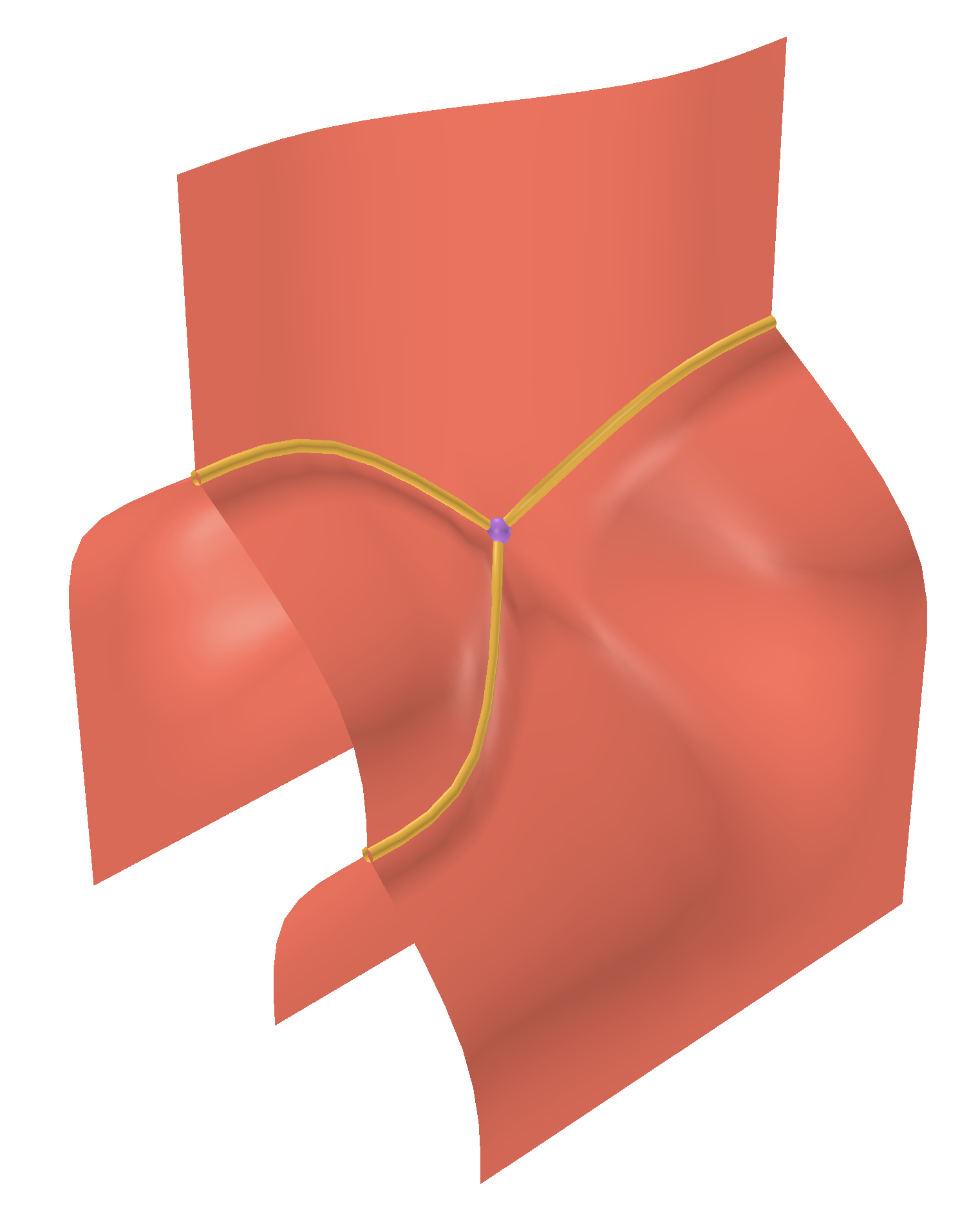
Figure 5: The associator 3-diagram as seen in homotopy.io.

Zigzag layout algorithm.

Given a finite poset-shaped diagram

$$X:J\to\operatorname{\mathsf{Zig}}(\mathbf{C})$$

we obtain a (fair) layout according to the following scheme:

1. Build the diagram $J\xrightarrow{X}\operatorname{\mathsf{Zig}}(\mathbf{C})\to\Delta\hookrightarrow\mathbf{Pos}$ which we denote by $P$.

2. Obtain its mono-epi injectification according to Theorem 3.9:

   Assume wlog that $Pi\subseteq\widehat{P}i$ for all $i\in J$ and $\widehat{P}i\subseteq\widehat{P}j$ whenever $i<j$.

3. Construct a linear programming problem using the following scheme:

   minimise $$w+\sum m_{i,j,p}$$

   subject to $$0\leq v_{i,p}\leq w (i\in J,\,p\in\widehat{P}i)\quad(\star)$$

   $$v_{i,q}-v_{i,p}\geq 1 (p<q\text{ in }\widehat{P}i)\quad(\ast)$$

   $$v_{i,q}-v_{i,p}\geq 1 (\epsilon_{i}(p)<\epsilon_{j}(q)\text{ in }Pi)\quad(\diamond)$$

   $$\lvert v_{i,p}-v_{j,p}\rvert\leq m_{i,j,p} (i<j)\quad({\dagger})$$

   $$v_{j,q}=\operatorname{avg}(\{v_{j,p}\mid p\in Pi,\,P_{i<j}(p)=q\}) (i<j,\,q\in Pj)\quad({\ddagger})$$

4. Extract the layout from the solution: $\lambda_{i}(p)\coloneqq v_{i,p}$ for $i\in J$ and $p\in Pi$.

The idea is as follows. The set $\widehat{P}i$ is a disjoint union of all $Pj$ for $j\leq i$. Therefore, we have a variable $v_{i,p}$ for every $p\in Pj$ for $j\leq i$. We think of this as the value of $\lambda_{j}(p)$ locally at $i$, with the true value being the one at $j$. This gives for each $i$ a local layout for the points in the neighbourhood of $i$. The constraints $({\dagger})$ assert that the local layouts agree on common points, whereas the constraints $({\ddagger})$ impose that each local layout is fair, and together, they imply that the global layout is fair. Of course, this would not be satisfiable, so the constraints $({\dagger})$ are weakened so that the difference between local layouts is minimised instead of made zero. This gives a layout that, while not fair, is as fair as possible.

4.2 Layout for diagrams

We can obtain a layout for any $n$-diagram $X$ recursively:

1. If $X$ is a 0-diagram, its layout is trivial:

   $$\lambda:\operatorname{\mathsf{pt}}^{0}(X) \to\mathbb{R}^{0}$$

   $$[] \mapsto()$$

2. If $X$ is an $(n+1)$-diagram, compute its layout as an $n$-diagram:

   $$\lambda_{\mathrm{ind}}:\operatorname{\mathsf{pt}}^{n}(X)\to\mathbb{R}^{n}$$

3. Construct its $n$-fold explosion $\operatorname{\mathsf{pt}}^{n}(X)\to\operatorname{\mathsf{Zig}}(\mathbf{C})$.

4. Obtain its layout using the zigzag layout algorithm:

   $$\lambda_{\mathrm{zig}}:\operatorname{\mathsf{pt}}^{n+1}(X)\to\mathbb{R}$$

5. Finally, combine this with the inductive layout to get a full layout for $X$:

   $$\lambda:\operatorname{\mathsf{pt}}^{n+1}(X) \to\mathbb{R}^{n+1}$$

   $$p \mapsto(\lambda_{\mathrm{zig}}(p),\lambda_{\mathrm{ind}}(\operatorname{tail}p))$$

Figure 6: A full layout for a 2-diagram (combining the layouts of Figures 3 and 4).

Appendix A Universal zigzag bundle

The zigzag construction can also be described as a polynomial functor. This is due to Heidemann [Hei23] and can be used to give an elegant defintion of explosion as a left adjoint of the zigzag construction.

Definition A.1.

The universal zigzag category $\mathbf{Z}$ is the category with singular objects $(n,\operatorname{\mathsf{s}}i)$ for $n\in\mathbb{N}$ and $0\leq i<n$, regular objects $(n,\operatorname{\mathsf{r}}j)$ for $n\in\mathbb{N}$ and $0\leq j\leq n$, and morphisms given by:

$$\mathbf{Z}((n,\operatorname{\mathsf{s}}i),(m,\operatorname{\mathsf{s}}j)) =\{f:\mathbf{n}\to\mathbf{m}\mid f(i)=j\}$$

$$\mathbf{Z}((n,\operatorname{\mathsf{r}}i),(m,\operatorname{\mathsf{r}}j)) =\{f:\mathbf{n}\to\mathbf{m}\mid\operatorname{\mathsf{R}}f(j)=i\}$$

$$\mathbf{Z}((n,\operatorname{\mathsf{r}}i),(m,\operatorname{\mathsf{s}}j)) =\{f:\mathbf{n}\to\mathbf{m}\mid\operatorname{\mathsf{R}}f(j)\leq i\leq\operatorname{\mathsf{R}}f(j+1)\}$$

$$\mathbf{Z}((n,\operatorname{\mathsf{s}}i),(m,\operatorname{\mathsf{r}}j)) =\varnothing$$

There is a canonical forgetful functor, called the universal zigzag bundle,

sending both $(n,\operatorname{\mathsf{s}}i)$ and $(n,\operatorname{\mathsf{r}}j)$. Now consider diagrams of the following form in $\mathbf{Cat}$:

If we let $\mathbf{J}=\mathbf{1}$, then $\mathbf{1}\to\Delta$ picks an object $n\in\mathbb{N}$. Then the fiber $\mathbf{Z}_{n}\coloneqq\mathbf{1}\times_{\Delta}\mathbf{Z}$ is a category representing the “shape” of a zigzag of length $n$, and a functor $\mathbf{Z}_{n}\to\mathbf{C}$ is precisely a zigzag of length $n$ in $\mathbf{C}$.

Proposition A.2.

The functor $p$ is exponentiable, i.e. the pullback functor $p^{*}$ has a right adjoint:

We can now recover the zigzag construction from (2) as the polynomial functor

where $\Sigma_{!}$ is the the left adjoint of $!_{*}$ (which always exists). In particular, we have an adjunction

$$\mathbf{Cat}/\Delta(\mathbf{J},\operatorname{\mathsf{Zig}}(\mathbf{C}))\cong\mathbf{Cat}(\mathbf{J}\times_{\Delta}\mathbf{Z},\mathbf{C}).$$

which is precisely the explosion construction; given $X:\mathbf{J}\to\operatorname{\mathsf{Zig}}(\mathbf{C})$, we have that $\operatorname{\mathsf{pt}}(X)\cong\mathbf{J}\times_{\Delta}\mathbf{Z}$.

References

- [Bur23] Simon Burton. String diagrams for higher mathematics with wiggle.py. Talk at SYCO 11, 2023.
- [BV17] Krzysztof Bar and Jamie Vicary. Data structures for quasistrict higher categories. In 32nd Annual ACM/IEEE Symposium on Logic in Computer Science, pages 1–12. IEEE, 2017.
- [CHH+23] Nathan Corbyn, Lukas Heidemann, Nick Hu, Chiara Sarti, Calin Tataru, and Jamie Vicary. The proof assistant homotopy.io, 2023.
- [DDV23] Christoph Dorn, Christopher Douglas, and Jamie Vicary. The theory of associative -categories. In preparation, 2023.
- [Dor18] Christoph Dorn. Associative -categories. PhD thesis, University of Oxford, 2018.
- [Hei23] Lukas Heidemann. Framed combinatorial topology with labels in -categories. In preparation, 2023.
- [HH18] Q. Huangfu and J. A. J. Hall. Parallelizing the dual revised simplex method. Mathematical Programming Computation, 10(1):119–142, 2018.
- [HRV22] Lukas Heidemann, David Reutter, and Jamie Vicary. Zigzag normalisation for associative -categories. In 37th Annual ACM/IEEE Symposium on Logic in Computer Science, pages 1–13. ACM, 2022.
- [KZ15] Aleks Kissinger and Vladimir Zamdzhiev. Quantomatic: a proof assistant for diagrammatic reasoning. In 25th International Conference on Automated Deduction, pages 326–336. Springer, 2015.
- [Rie08] Emily Riehl. Factorization systems. Notes from a talk, 2008.
- [RV19] David Reutter and Jamie Vicary. High-level methods for homotopy construction in associative -categories. In 34th Annual ACM/IEEE Symposium on Logic in Computer Science, pages 1–13. IEEE, 2019.
- [SWZ19] Paweł Sobociński, Paul W Wilson, and Fabio Zanasi. Cartographer: a tool for string diagrammatic reasoning. In 8th Conference on Algebra and Coalgebra in Computer Science, pages 1–7, 2019.
- [Wra93] Gavin C Wraith. Using the generic interval. Cahiers de topologie et géométrie différentielle catégoriques, 34(4):259–266, 1993.