XUV emission of the young planet-hosting star V1298 Tau from coordinated observations with XMM-Newton and HST
Abstract
Atmospheric mass loss plays a major role in the evolution of exoplanets. This process is driven by the stellar high-energy irradiation, especially in the first hundreds of millions of years after dissipation of the proto-planetary disk. A major source of uncertainty in modeling atmospheric photo-evaporation and photo-chemistry is due to the lack of direct measurements of the stellar flux at EUV wavelengths. Several empirical relationships have been proposed in the past to link EUV fluxes to emission levels in X-rays, but stellar samples employed for this aim are heterogeneous, and available scaling laws provide significantly different predictions, especially for very active stars. We present new UV and X-ray observations of V1298 Tau with HST/COS and XMM-Newton, aimed to determine more accurately the XUV emission of this solar-mass pre-Main Sequence star, which hosts four exoplanets. Spectroscopic data were employed to derive the plasma emission measure distribution vs. temperature, from the chromosphere to the corona, and the possible variability of this irradiation on short and year-long time scales, due to magnetic activity. As a side result, we have also measured the chemical abundances of several elements in the outer atmosphere of V1298 Tau. We employ our results as a new benchmark point for the calibration of the X-ray to EUV scaling laws, and hence to predict the time evolution of the irradiation in the EUV band, and its effect on the evaporation of exo-atmospheres.
1 Introduction
The frequency of planets as a function of their masses, size, and host star properties is a key parameter for testing planet formation and evolution models. On the other hand, evolutionary paths are the result of a complex interplay between physical and dynamic processes operating on different time scales, including the stellar radiation fields. In particular, intense high-energy irradiation from the host stars, especially at young ages, can be responsible for atmospheric evaporation of the exoplanets, and it is one of the ingredients, still poorly understood, that shapes the planet mass-radius relationship (Lopez & Fortney 2013; Owen & Wu 2013; Fulton et al. 2017; Owen & Wu 2017; Fulton & Petigura 2018; Owen & Lai 2018).
The thermal structure and chemistry of planetary atmospheres sensitively depend on the spectral energy distribution of the stellar radiation (Lammer et al., 2003). While EUV photons are absorbed in the upper atmosphere, soft X-rays can heat and ionize lower layers due to secondary electron production (Cecchi-Pestellini et al., 2006). A reliable characterization of planetary evolution requires the knowledge of the stellar XUV emission (5–920 Å range) and its variation with stellar age (Sanz-Forcada et al. 2011; Locci et al. 2019).
Planets in close orbits around young stars are especially susceptible to the effects of irradiation because the host stars are known to have higher magnetic activity levels relative to the Sun. Higher XUV fluxes are generally accompanied by more frequent and energetic flares, and conjectured higher rates of Coronal Mass Ejections (CMEs, Khodachenko et al. 2007). In turn, charged particle flows linked to stellar winds and CMEs determine the size and time-dependent compression of planetary magnetospheres, and eventually may lead to stripping (erosion) of close-in planets (Lammer et al., 2007), as well as deposition of gravity waves (Cohen et al., 2014).
High energy radiation (including X-rays, Extreme UV, and Far UV bands) originates from stellar outer atmospheres. In particular, plasmas in the temeprature range T K produces FUV emission lines, while X-ray spectral lines and continuum emission are tipically formed where temperatures rise above K. Significant flux in the EUV band originates from plasma with temperatures in the whole range K.
The goal of coordinated observations at X-rays and UV wavelengths is to provide a benchmark for models of photo-evaporation and photo-chemistry of exoplanets, especially at young ages. Measurements of the hardness, fluence, and variability of the XUV irradiation, can be connected to masses, sizes and atmospheric chemical composition, acquired with observations from ground and space-borne facilities.
Here we present a detailed study of the young star V1298 Tau, simultaneously observed at UV wavelengths with HST/COS and in X-rays with XMM-Newton.
This target represents a unique study case, because it is a young solar analogue hosting a compact planetary system, with four planets at distances between 0.08 and 0.3 AU from the host star, which implies more than a factor 10 difference in XUV irradiation. Hence, the system provides a valuable benchmark for planet migration and evolution models, and rich prospects for atmospheric characterization by transmission spectroscopy.
In this paper we introduce first the characteristics of the host star and its planetary system (Sect. 2). Next, we present new HST/COS and XMM-Newton observations of the host star (Sect. 3), performed simultaneously, with the aim to reconstruct the stellar spectrum over a wide wavelength range, extending from 5 Å to 1450 Å. Then, we describe our reconstruction of the transition region and coronal plasma distribution vs. temperature, and revise the most likely radiation budget at EUV wavelengths (Sect. 4.3). Finally, we compare our results to predictions based on X/EUV scaling laws proposed in the past, and we draw attention on their accuracy and limitations (Sect. 5).
2 Stellar characteristics
V1298 Tau is a K1 star with a mass of M⊙, a radius of R⊙, an effective temperature K, and a bolometric luminosity L⊙ (Suarez Mascareño et al., 2021). It is located at a distance of pc (Gaia Collaboration, 2020, DR3) toward the Taurus region, and it belongs to the Group 29 stellar association (Oh et al., 2017). For V1298 Tau we determined an age of Myr (Maggio et al., 2022).
V1298 Tau hosts one of the youngest planetary systems known so far, discovered with the Kepler K2 mission (David et al., 2019). The system counts two Neptune-sized planets (dubbed ”c” and ”d”), one Jovian planet (”b”), and one Saturn-sized planet (”e”), in order of increasing separation from the central star (Suarez Mascareño et al., 2021).
Possible alternative evolutionary paths of the planetary masses and sizes, due to photoevaporation of the primary atmospheres, were explored by Poppenhaeger et al. (2021), based on a X-ray snapshot with Chandra, and by Maggio et al. (2022), based on a first observation of V1298 Tau with XMM-Newton, performed in February 2021.
3 Observations and data analysis
3.1 XMM-Newton observation
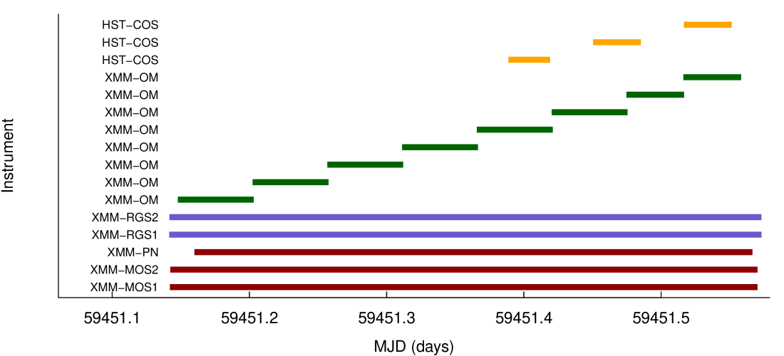
A new XMM-Newton observation of V1298 Tau was performed on 2021 August 25 (ObsId 0881220101, PI S. Benatti), in order to characterize the X-ray emission and variability of the host star. The exposure time was about 36 ks with EPIC as a prime instrument in full frame window imaging mode and with the Medium filter. We also acquired data from RGS and OM instruments simultaneously.
The Observation Data Files (ODFs) were reduced with the Science Analysis System (SAS, ver.20.0.0), following standard procedures. We obtained FITS tables of X-ray events detected by the three EPIC CCD cameras (MOS1, MOS2, and pn) and with the two high-resolution spectrographs (RGS1 and RGS2), calibrated in energy, arrival times and astrometry by means of the emchain/epchain SAS tasks. Inspection of the light curve of events detected with energies keV allowed us to identify and filter out several time intervals affected by high background.
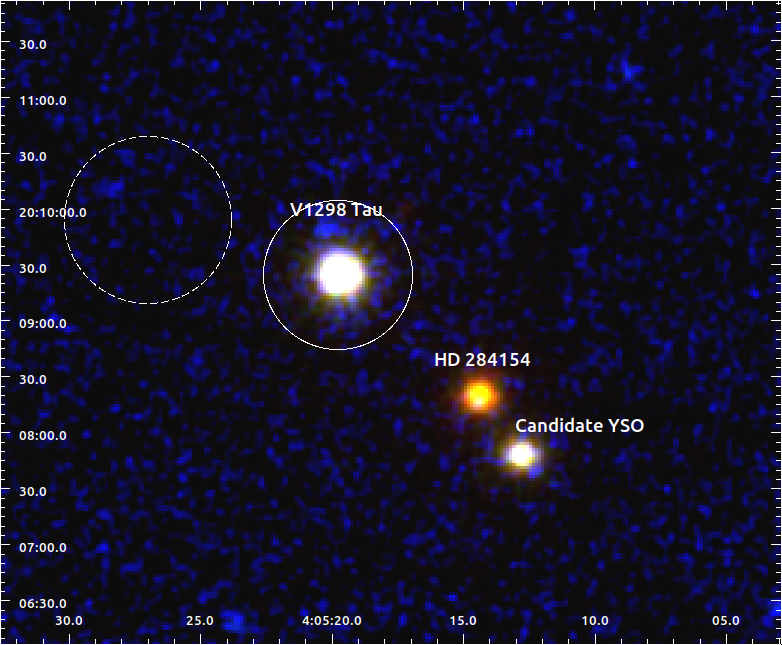
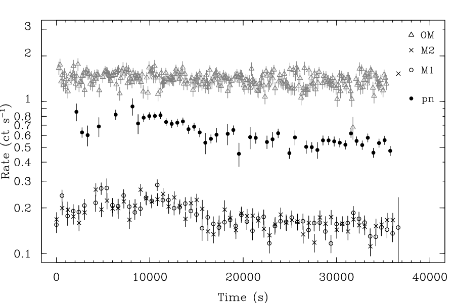
V1298 Tau is sufficiently isolated to allow the extraction of the source signal from a circular region of 40″radii for MOS and pn, and local background from an uncontaminated nearby circular region of similar size. With SAS we also produced the response matrices and effective area files needed for the subsequent spectral analysis. RGS source and background spectra were also extracted adopting the standard results of the SAS pipeline. Source X-ray spectra and light curves are shown in Fig. 3. In the same figure, we show the OM light curve, obtained with the SAS task omfchain.
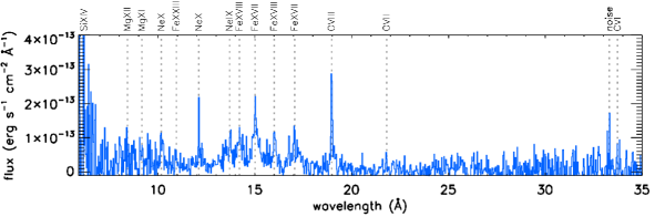
For measurements of X-ray line fluxes we considered the spectrum obtained by adding the 1-st order RGS1 and RGS2 spectra, which cover the Å range, with an average resolution of 0.06 Å FWHM. For improving the statistics, we also co-added the RGS spectra obtained in Aug 2021 with those already available from the previous XMM-Newton observation, taken in Feb 2021 (Maggio et al., 2022) ( ks of clean exposure time), and we rebinned the resulting spectrum by a factor of 3 (Fig. 4). This choice is supported by the lack of strong variability of the coronal emission (Sect.4.2).
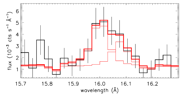
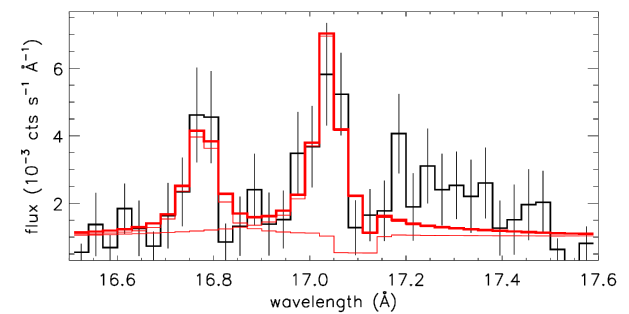
We identified the strongest emission lines and measured their fluxes by fitting the observed spectrum in small wavelength intervals. To model the line profile we used the RGS line spread function tabulated in the RGS response matrix file. The width of each wavelength interval was set to include blended lines that needed simultaneous fitting. In the best-fitting function, in addition to individual line contributions, we included also a continuum component, with temperature and normalization left free to vary. Because of the small width of the selected wavelength intervals, the continuum component, acting as an additive constant, takes into account also the integrated contribution of unresolved weak lines. Two examples of RGS line fitting are plotted in Fig. 5. The measured line fluxes are listed in Table 1. The observed X-ray lines form in the temperature range –16 MK, probing the thermal structure of the stellar corona.
3.2 HST observations
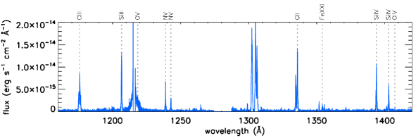
V1298 Tau was observed with HST during three consecutive orbits to acquire spectra in FUV with the COS spectrograph. The central wavelength was 1291Å covering about the 1150 – 1450 Å wavelength range. About 55 minutes were available during each orbit for science and acquisition exposures of V1298 Tau. The actual exposure times were 2249.2 s, 2634.1 s, and 2634.2 s, respectively, during the three orbits totalling about 7517.5 s. The orbits were simultaneous with the second half of the XMM-Newton observation during which the star appears quiescent in X-rays. The standard calibration operated with CalCOS (v. 3.3.10) at STScI was deemed sufficient and thus the reduced spectra were downloaded from the HST archive and ready for the subsequent analysis. The archive provides the spectra accumulated during each orbit and their average spectrum. We checked that the ion lines have similar intensities during each orbit. Since the star was quiescent in X-rays, we determined to analyze the average spectrum (Fig. 6) so to maximize the count statistics.
We identified and measured the strongest UV emission lines in this averaged spectrum. Line fluxes were obtained by fitting the observed spectrum in small wavelength intervals, assuming for the line profile a beta-model (also known as Moffat line profile)
| (1) |
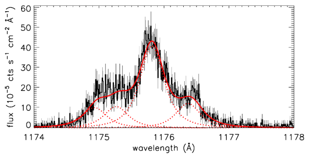
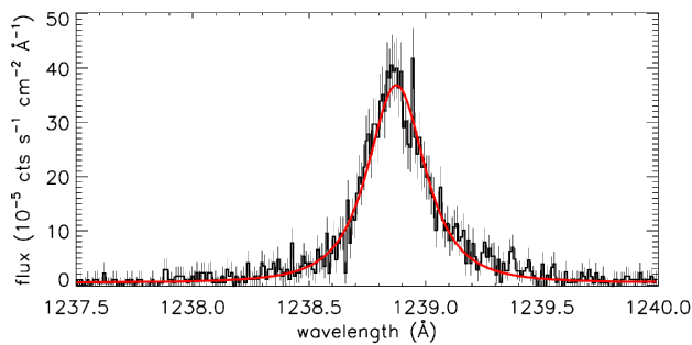
with Å and kept as fixed parameters. We adopted this line shape and parameters after having checked that this function reproduces well the observed line profile of strong and isolated lines. The width of the selected wavelength intervals was set to eventually include blended lines, for which simultaneous fitting is needed. We also included a constant function in addition to the line contributions in each interval, to fit also the continuum level. Two examples of COS line fitting are shown in Fig. 7, and the case of a few lines possibly altered by opacity effects are described in Appendix A.
Besides our Aug 2021 HST/COS G130M observation, we have also considered a previous observation of V1298 Tau taken with the G160M grating on 2020 Oct 17 (ObsId lebw02koq, PI P.W. Cauley), and available in the MAST archive. The aim was to measure the flux of the C IV doublet at Å, which is important to better constrain the thermal structure of the stellar chromosphere (Sect. 4.3). Since this observation was acquired in a different epoch, we checked again for the presence of variability by comparing the fluxes of the Si IV doublet at Å which is present in both the 2021 and 2020 spectra. As a result, we corrected this effect by dividing the C IV flux by a factor of 2.7.
All the measured line fluxes are listed in Table 1. This list comprises UV lines that form in the temperature range K, thus probing the thermal structure of the high chromosphere and the transition region of the star. In the same list we reported also the fluxes of a couple of lines with no clear identification. We instead did not include some O I emission lines, usually present in COS spectra, because of their geocoronal contamination.
| Ionb | EMD1e | EMD2e | ||||||
|---|---|---|---|---|---|---|---|---|
| 6.18 | Si XIV Si XIV | 7.20 | 610 | 250 | 1.43 | |||
| 8.42 | Mg XII Mg XII | 7.00 | 56 | 49 | -0.39 | -0.56 | ||
| 9.17 | Mg XI | 6.80 | 64 | 41 | 0.41 | 0.30 | ||
| 10.24 | Ne X Ne X | 6.80 | 117 | 32 | 1.59 | 2.59 | ||
| 10.98 | Fe XXIII Ne IX Fe XXIII Na X Fe XVII | 7.20 | 102 | 42 | 1.1 | 1.67 | ||
| 12.13 | Ne X Ne X Fe XVII Fe XXIII | 6.75 | 254 | 55 | -3.20 | -0.23 | ||
| 12.28 | Fe XXI Fe XVII | 7.05 | 97 | 40 | 1.06 | 0.28 | ||
| 13.45 | Ne IX Fe XIX Fe XIX | 6.60 | 71 | 40 | -2.07 | -0.98 | ||
| 13.52 | Ne IX Fe XIX Fe XIX Fe XXI | 7.00 | 91 | 37 | 0.12 | 0.08 | ||
| 13.70 | Ne IX | 6.55 | 161 | 40 | 1.83 | |||
| 14.20 | Fe XVIII Fe XVIII | 6.90 | 93 | 26 | -0.48 | 0.11 | ||
| 15.01 | Fe XVII | 6.75 | 188 | 30 | 0.97 | 0.98 | ||
| 15.08 | Fe XIX | 6.95 | 64 | 25 | 2.01 | 2.06 | ||
| 15.21 | Fe XIX O VIII O VIII | 6.95 | 63 | 32 | 1.11 | 1.61 | ||
| 15.26 | Fe XVII | 6.75 | 31 | 27 | -0.60 | -0.50 | ||
| 16.00 | Fe XVIII O VIII O VIII | 6.90 | 103 | 24 | 1.25 | 2.97 | ||
| 16.07 | Fe XVIII Fe XIX | 6.90 | 58 | 22 | 0.65 | 0.24 | ||
| 16.78 | Fe XVII | 6.75 | 82 | 24 | -0.41 | -0.17 | ||
| 17.05 | Fe XVII Fe XVII | 6.75 | 204 | 33 | -0.54 | 0.23 | ||
| 18.63 | O VII | 6.35 | 8 | 12 | -0.35 | 0.59 | ||
| 18.97 | O VIII O VIII | 6.50 | 373 | 34 | 3.65 | 9.77 | ||
| 21.60 | O VII | 6.30 | 37 | 32 | -1.04 | 0.92 | ||
| 21.81 | O VII | 6.30 | 77 | 35 | 1.97 | |||
| 22.10 | O VII | 6.30 | 61 | 27 | 0.60 | |||
| 33.73 | C VI C VI | 6.15 | 38 | 27 | 0.03 | 0.22 | ||
| 1174.93 | C III | 4.95 | 9.6 | 0.8 | 0.48 | |||
| 1175.26 | C III | 4.95 | 10.2 | 1.1 | 3.23 | |||
| 1175.71 | C III C III C III | 4.95 | 39.1 | 1.1 | -1.55 | -1.51 | ||
| 1176.37 | C III | 4.95 | 11.6 | 0.8 | 4.00 | |||
| 1206.50 | Si III | 4.80 | 67.3 | 1.1 | ||||
| 1218.35 | O V | 5.35 | 6.9 | 1.1 | -3.12 | -0.50 | ||
| 1238.82 | N V | 5.30 | 21.5 | 1.1 | 0.09 | -0.13 | ||
| 1242.81 | N V | 5.30 | 11.8 | 0.9 | 1.16 | 1.26 | ||
| 1253.81 | S II | 4.50 | 0.9 | 0.3 | -0.02 | -0.40 | ||
| 1264.74 | Si II Si II | 4.45 | 4.2 | 0.3 | 2.44 | |||
| 1266.11 | … | 0.00 | 1.1 | 0.2 | ||||
| 1294.55 | Si III | 4.80 | 1.1 | 0.3 | 2.68 | |||
| 1298.95 | Si III Si III | 4.80 | 3.0 | 0.6 | 3.71 | |||
| 1309.28 | Si II | 4.45 | 1.6 | 0.3 | -2.31 | |||
| 1323.95 | C II C II C II | 4.75 | 0.8 | 0.3 | -0.57 | 0.71 | ||
| 1334.53 | C II | 4.60 | 32.7 | 0.9 | -27.91 | -1.84 | ||
| 1335.71 | C II C II | 4.60 | 69.5 | 1.2 | 27.99 | 1.41 | ||
| 1351.44 | … | 0.00 | 3.3 | 0.6 | ||||
| 1354.07 | Fe XXI | 7.05 | 5.5 | 0.5 | 0.88 | -0.67 | ||
| 1364.22 | … | 0.00 | -0.4 | 0.3 | ||||
| 1371.30 | O V | 5.35 | 1.9 | 0.4 | -1.56 | 4.55 | ||
| 1393.76 | Si IV | 4.90 | 41.6 | 2.6 | -2.54 | -1.42 | ||
| 1401.16 | O IV | 5.15 | 3.4 | 0.5 | -23.68 | -0.99 | ||
| 1402.77 | Si IV | 4.90 | 23.6 | 0.9 | -0.59 | 1.65 | ||
| 1407.38 | O IV | 5.15 | 0.6 | 0.3 | -0.47 | |||
| 1548.19 | C IV | 5.05 | 83.0 | 2.4 | 0.87 | -0.73 | ||
| 1550.78 | C IV | 5.05 | 44.8 | 2.0 | 0.91 | 1.57 | ||
a Wavelengths (Å). b Multiple identifications indicate unresolved lines in the CHIANTI database which contribute to the measured flux. c Temperature (K) of maximum emissivity. d Measured fluxes () with uncertainties at the 68% confidence level. e Lines selected for the EMD reconstruction with each method. f Comparison between observed and predicted line fluxes (method 1). g Comparison between observed and predicted line fluxes (method 2).
3.3 HARPS-N observations
We observed V1298 Tau within a dedicated DDT program (ID: A42DDT5, PI: A. Maggio) at the Telescopio Nazionale Galileo (TNG, La Palma, Canary Islands) by using the HARPS-N high-resolution spectrograph (Cosentino et al., 2014) in the visible band (383 - 690 nm). We obtained six spectra of the target between Feb 23rd and Feb 26th, 2021, in order to perform a follow-up of the first XMM-Newton observation through the monitoring of the chromospheric emission in the Ca II H&K lines. Three additional spectra of V1298 Tau were collected between Aug 23rd and Aug 26th to support the coordinated XMM-Newton-HST observation within the Global Architecture of Planetary Systems (GAPS) project. Since V1298 Tau was also included in the Young Objects sample of GAPS (Carleo et al., 2020), a large amount of data (almost 190 spectra between Mar 2019 and Mar 2022) has been collected by this observing program, aiming to measure the masses of the four planets of the system. For all datasets, we calculated the values of the activity index by using the procedure described in Lovis et al. (2011, and references therein) available on the YABI workflow interface, implemented at the INAF Trieste Observatory111https://www.ia2.inaf.it/.
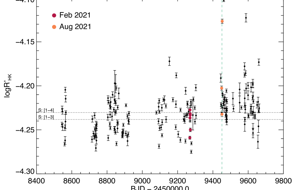
The use of the GAPS data allows us to perform a comparison of the values of obtained during the XMM-Newton-HST observations with its typical behaviour over four years. Fig.8 shows the time series of this chromospheric activity index obtained as part of the GAPS program (black dots), and the values taken during the DDT program in Feb 2021 (red dots) and the additional observations in Aug 2021 (orange dots). No significant difference is visible between our first set of DDT data and the GAPS ones, since the chromospheric indexes appear well within the mean distribution. Instead, we observe an excess in the value of () for one spectrum of the second set of DDT data (on 2021 Aug 26 at 05:16 UT) and for two GAPS spectra (on 2021 Sep 4 at 04:51 UT, and on 2022 Jan 08 at 01:03 UT, respectively). We note that the mean value of the appears slightly larger in the last season than in the previous ones, as indicated by the median values drawn in Fig. 8 as horizontal lines, suggesting an enhancement of the stellar activity, in full agreement with what we found in X-rays. We hypothesize that the spectra showing the highest values of could have caught the star during large stellar flares. For a double check, we extracted the H index from those spectra by using the ACTIN code (Gomes da Silva et al., 2018). Actually, we observed a higher value also for this chromospheric proxy, which corroborates the flare hypothesis (see e.g. Di Maio et al. 2020), although the optical spectra show no significant emission in the H line core.
Finally, we used a subset of these HARPS-N data to obtain a co-added spectrum aiming to perform a comparison between the photospheric abundances with those in the outer stellar atmosphere probed by the XUV lines. To derive an estimate of the metallicity we performed the comparison with synthetic spectra (calculated using MOOG and a grid of Kurucz model atmospheres), which include Fe I lines. We obtained T K, dex, km/s, and the resulting [Fe/H] is dex (with , in agreement with the solar abundance reported by Suárez Mascareño et al. (2021). The combination of relatively high rotational velocity and low effective temperature prevents us from deriving accurate abundances of other elements, because of possible unknown line blending and NLTE effects for carbon, silicon, and magnesium (see also Suárez Mascareño et al. 2021).
4 Results
4.1 Source variability
The EPIC X-ray light curves of V1298 Tau (Fig. 3) show low-level but significant time variability in the first 15 ks of the Aug 2021 XMM-Newton observation, with a peak count rate % higher with respect to the average quiescent level observed in the next 21 ks time segment. This behavior is more clear in the MOS light curves, less affected by high background contamination than pn. The simultaneous NUV light curve obtained with the OM shows just some flickering at the level of % with respect to the average count rate.
Although no large flare is evident, we analyzed separately the EPIC spectra accumulated in the two time segments, which we dubbed ”quiescent” and ”high-state”, in order to check for possible variations of the characteristics of the coronal plasma. Further assessment of the long-term variability of V1298 Tau is postponed to the end of Sect.4.2.
| Obs Id | T1 | EM1 | T2 | EM2 | T3 | EM3 | d.o.f. | Abundances and 90% confidence ranges (solar units; Anders & Grevesse 1989) | ||||||||||||
|---|---|---|---|---|---|---|---|---|---|---|---|---|---|---|---|---|---|---|---|---|
| K | cm-3 | K | cm-3 | K | cm-3 | erg s-1 cm-2 | erg s-1 | Mg | Fe | Si | S | C | O | N | Ca | Ne | ||||
| 7.65 | 7.90 | 8.15 | 10.36 | 11.26 | 13.62 | 14.53 | 15.76 | 21.56 | ||||||||||||
| Feb 2021 | 532.8 | 431 | 0.33 | 0.17 | 0.25 | = O | =O | 0.29 | =O | = Ne | 0.95 | |||||||||
| Quiescent | 605.0 | 510 | 0.19 | 0.10 | 0.10 | = O | =O | 0.22 | =O | = Ne | 0.47 | |||||||||
| High-state | 474.8 | 422 | 0.25 | 0.19 | 0.08 | = O | =O | 0.38 | =O | = Ne | 0.65 | |||||||||
| Combined | 1645.6 | 1315 | 0.21 | 0.13 | 0.15 | 0.26 | =O | 0.28 | =O | = Ne | 0.61 | |||||||||
| 0.32 | 0.13 | 0.81 | 0.23 | 0.18 | 0.20 | 0.41 | 0.91 | |||||||||||||
| 0.41 | 0.15 | 1.49 | 0.35 | 0.25 | 0.03 | 0.23 | 0.59 | |||||||||||||
Note. — Unabsorbed X-ray flux and luminosity in the 0.1–10 keV band. Errors are quoted at the 90% confidence level.
4.2 Global fitting of X-ray spectra
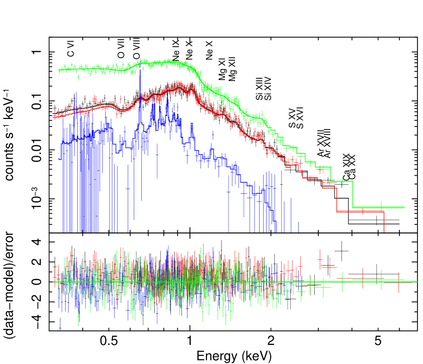
For the spectral analysis, performed with xspec V12.12.0, we proceeded as in Maggio et al. (2022). Initially we applied a best-fitting procedure only to the EPIC (MOS1, MOS2, and pn) X-ray spectra. We adopted an optically-thin coronal emission model (AtomDB v3.0.9, Foster et al. 2012) composed of three isothermal components (3T, vapec), with the abundances of all elements linked to the iron abundance. Next, we added also the combined RGS1 and RGS2 high-resolution spectra, and allowed up to nine elements as free parameters: C, N, O, Ne, Mg, Si, S, Ar, and Fe. A global interstellar absorption was also included in the model with a multiplicative component (phabs).
Eventually, we reduced the number of free parameters by fixing the interstellar hydrogen column density, , and the abundances of C, N and Ar, because these parameters were poorly constrained. In fact, the best-fit value of was consistent with the value derived from the known B-V color excess, (David et al. 2019), which implies an extinction and cm-2, hence we fixed this parameter to the nominal value. Similarly, the best-fitting procedure yields just uninformative upper limits for both the C and N abundances, and we decided to fix both of them to the Oxygen abundance, guided by the similarity of the First Ionization Potentials of these elements (see 4.4). The line complex of Ar XVII and Ar XVIII at 3.14 keV and 3.32 keV, respectively, is quite evident in the combined spectrum (Fig. 3), and the best-fit abundance is near the solar value, but we fixed it to the abundance of Neon due to the large uncertainties.
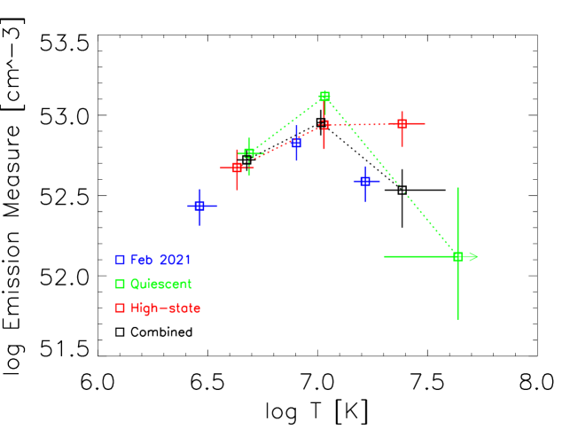
Table 2 reports the parameters from the best-fit models to EPIC and RGS spectra of the ”quiescent” and ”high-state” time segments. We also show the results of the fitting of the Feb 2021 spectra and of the combined spectra obtained by adding the Feb 2021 and Aug 2021 data, performed with the same procedure. During the Aug 2021 observation, the coronal plasma of V1298 Tau was characterized by a cold temperature component at 4–5 MK, and a second component at 10 MK. The volume emission measures of these components did not change appreciably from the ”quiescent” to the ”high-state” phase, and they appear similar also to those probed by the Feb 2021 observation. Moreover, there is evidence in all cases of very hot plasma, at 15–25 MK, which is responsible for most of the observed variability: this component has a very low emission measure during the ”quiescent” phase in Aug 2021, while it becomes the dominant one during the ”high-state” phase. A comprehensive view of the results of these multi-component isothermal fitting of the XMM spectra is displayed in Fig.9. This is typical behavior for the variability of the coronal plasma in young active stars.
The unabsorbed flux and the luminosity of V1298 Tau in the quiescent phase are erg s-1 cm-2 and erg s-1, respectively in the band 0.1–2.4 keV. These values are about 20% higher than those observed in Feb 2021. A further increase of % occurred during the variable phase in Aug 2021, characterized by an average flux and luminosity of erg s-1 cm-2 and erg s-1. A slightly larger variability can be derived in the broader X-ray band 0.1–10 keV (Table 2). Considering also previous ROSAT and Chandra observations (Poppenhaeger et al., 2021), the X-ray emission of V1298 Tau shows a long-term variability within a factor .
Finally, we evaluated that the X-ray to bolometric luminosity ratio, , ranged from -3.35 to -3.15 in the time span between Feb 2021 and Aug 2021, and the flux at the stellar surface, , was between and erg s-1 cm-2. These surface fluxes are 10–100 times higher than in the case of the Sun at the maximum and minimum of its magnetic activity cycle (Chadney et al., 2015).
The significant but low-amplitude variability of V1298 Tau is also confirmed by considering the 3-year time series of the chromospheric Ca II H&K emission lines (Fig.8), where the index shows a full range of variation dex. These measurements can be converted into the pure activity-related R index by Mittag et al. (2013), and we have employed the latter to predict the X-ray to bolometric luminosity ratios by means of the chromospheric to coronal flux-flux relationship derived by Fuhrmeister et al. (2022) for active G-type stars. We found a full range of between and , i.e. a possible variability of about a factor 3.
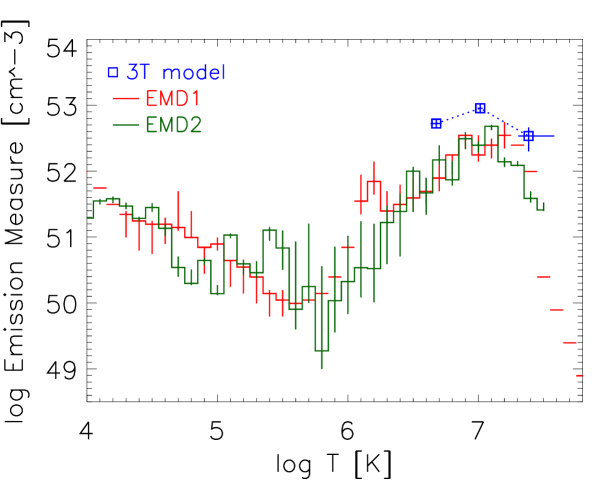
4.3 Emission Measure Distribution
The full set of UV and X-ray line fluxes probes emission from material with temperatures ranging from K to K. This line set allows us to derive the Emission Measure Distribution (EMD) vs. temperature of the entire stellar atmosphere, from the chromosphere to the corona. To this aim, we assume that the emission is due to a collisionally-excited optically-thin plasma. We have checked that deviations from this hypothesis affect only marginally some strong lines which form at chromospheric temperatures (see Appendix A).
The lack of significant variability of the chromospheric index and of the coronal emission between Feb 2021 and Aug 2021 observations (Sect. 4.1), except for the thermal components hotter than MK, supports our assumption that the same occurred for the strength of the EUV emission lines.
Interstellar absorption, assuming cm-2, was properly taken into account for computing unabsorbed X-ray line fluxes, while we have employed the Fitzpatrick (1999) extinction law for the UV lines.
We employed two different and independent methodologies for the reconstruction of the EMD vs. temperature. We have first derived the EMD following Sanz-Forcada et al. (2003b) (Method 1). An initial EMD with 0.1 dex resolution in temperature, based on global fitting results, is used to calculate the expected line fluxes for the source. These calculations include contributions from all lines in identified blends, according to the AtomDB (v3.0.9) database. The ratio between observed and predicted line fluxes is used to modify the EMD and the abundances of the elements in an iterative process, thus obtaining the best result to minimize these line ratios. The EMD is computed initially using abundances relative to iron. At the end of the process, the whole EMD is shifted by +0.89 dex, to correct for the value determined with the global fitting of the combined spectrum (Sect. 4.2). The method provides also uncertainties on both EMD and abundances with a MonteCarlo method which takes into account the uncertainties on the measured line fluxes, but keeping fixed the iron abundance.
In this process, special attention was made to the consistency of spectral line fluxes of similar ions or temperature of formation, excluding some of them (e.g. Si III 1206.50 Å). A special treatment was also applied to the C III multiplet at Å, having inaccurate atomic data in AtomDB v3.0.9. In this case, we adopted the Raymond (1988) atomic data to evaluate the flux of the whole multiplet.
Then, we derived an alternative solution for the plasma EMD and abundances by employing the MCMC approach implemented in the PINTofALE software suite (v2.954) (Kashyap & Drake, 1998). In applying this procedure (Method 2) we adopted the CHIANTI (v7.13) atomic database, since it appears more reliable than APEC in reproducing some strong lines in the UV range. We considered a subset of measured line fluxes, as reported in Table 1. In particular, we did not consider density-sensitive lines, lines with uncertain identification, and lines whose fluxes appear incompatible among themselves in the hypothesis of collisionally-excited plasma222This issue occurred for some Si lines in the UV band, possibly because the population of the upper levels from which they originate have significant contributions also from other mechanisms, like recombination.. To obtain absolute abundances and to better constrain the hottest components of the EMD we complemented these selected line fluxes with the measurements of the total flux (lines + continuum) in five wavelength intervals, including also intervals at short wavelengths where the emission is dominated by the hot plasma (Pillitteri et al. 2022). To this aim we selected the intervals reported in Table 3. The observed fluxes in these intervals were obtained from the EPIC data with XSPEC. We computed the total emissivities associated to these measurements including, in addition to the continuum contribution, the contribution of all the emission lines contained in the considered wavelength interval. We run the MCMC procedure several times, adjusting at each step this emissivity on the basis of the inferred abundances.
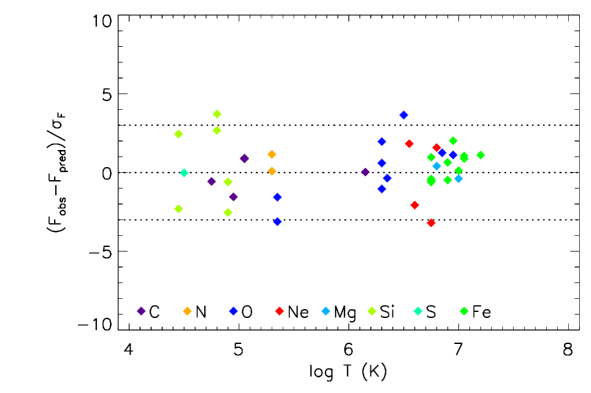
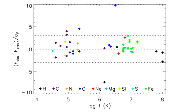
Considering the temperature ranges covered by the emissivities of the selected lines, we derived the EMDs over a temperature grid ranging from to , with . The results are shown in Fig.10, together with plots of the residuals between observed and predicted line fluxes with the two methods (Tab. 1).
The EMD obtained with method 1 appears smoother than the other, but the two solutions turned out to be consistent within uncertainties, except for a few bins, in spite of a slightly different set of emission lines and methodologies of EMD reconstruction. Note that method 1 joins the estimated emission measure values between and 6.1 K with a few bins without formal errors, because this is the temperature range less constrained by the available UV and X-ray emission lines. The same occurs for the EMD at K. Method 2 extends the reconstructed EMD up to K thanks to the inclusion of the narrow band X-ray fluxes which inform on the continuum emission level. Moreover, the 0.1–2.4 keV broad band flux and the Li-like lines of C and N have emissivity functions with significant contributions also from plasma in the range 5.5–5.9 K. It is because of these emissivities that the EMD can be constrained with Method 2 also in this temperature range, although with large error bars.
In Appendix B we show a comparison of the EMD of V1298 Tau with those of other G–K stars having different activity levels.
| 2.48– | 4.13 | 3.00– | 5.00 | 8.00 | 46.8 | 2.9 | -0.76 |
| 4.13– | 5.17 | 2.40– | 3.00 | 8.00 | 39.2 | 1.9 | -2.79 |
| 8.49– | 8.92 | 1.41– | 1.46 | 7.80 | 14.9 | 0.3 | -0.49 |
| 27.55– | 30.24 | 0.41– | 0.45 | 6.55 | 28.6 | 0.5 | 0.47 |
| 5.17– | 123.99 | 0.10– | 2.40 | 6.15 | 1040.0 | 10 | -7.34 |
| – | |||||||
a Wavelength range (Å).
b Energy range (keV).
c Temperature (K) of maximum emissivity.
d Observed fluxes ().
e Comparison between observed and predicted line fluxes.
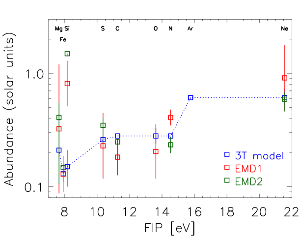
4.4 Chromospheric and coronal abundances
The elemental abundances in the corona of V1298 Tau, derived from the global analysis of the combined XMM-Newton spectra (Sect. 4.2), are shown in Fig.11 as a function of the First Ionization Potential (FIP). Similar values were obtained also for the single observations in Feb 2021 and Aug 2021, as well as for the quiescent and high-state segments (Tab. 2). Elements with low FIP (Fe, Mg, and Si) are systematically underabundant with respect to elements with eV, such as O, N, or Ne. This trend, dubbed inverse FIP effect, is typical of young active stars (Maggio et al., 2007; Scelsi et al., 2007).
In the same figure are shown the values derived together with the EMDs, which resulted in fair agreement with the values from the global fitting of X-ray spectra, except for the case of Silicon. In this case, we are assuming that the abundances of elements such as O and Si remain constant in the full range of temperatures explored, but we recognize that the abundances could change somewhere between the chromosphere and the corona. Moreover, some differences may be due to the two different atomic databases employed for the analysis of the emission lines.
We recall also that the abundances of V1298 Tau in the chromosphere and corona are scaled with respect to the solar photospheric abundances (Anders & Grevesse, 1989). Stellar abundances for each element should be employed for a proper assessment of any trend with the FIP (Sanz-Forcada et al., 2004), but unfortunately, accurate photospheric abundances cannot be determined for V1298 Tau(Sect.3.3), except for the iron. In this latter case, the difference between the photosphere and the corona is clearly established.
4.5 EUV vs. X-ray scaling laws
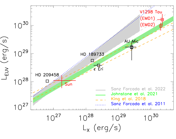
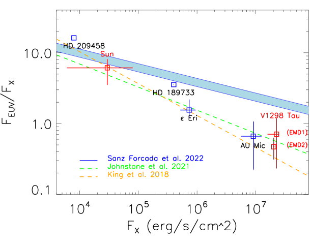
We have employed the EMDs presented above to compute the X-ray luminosity in the 5–100 Å band, and the EUV luminosity in the 100–920 Å band. We have obtained erg s-1 and erg s-1 with method 1, and erg s-1 and erg s-1 with method 2. The uncertainties on luminosities from method 2 were evaluated from the luminosity distributions obtained from the Monte Carlo sampling of the and abundances parameter space. In the case of method 1, we assume an uncertainty on equal to the range measured between the Feb 2021 observation and the high-state at the Aug 2021 epoch, which is 1.6 – erg s-1 in the 5–100Å band, while the uncertainty on the EUV luminosity was computed by generating the spectra relative to the upper and lower boundaries of the EMD range.
In Fig.12 we plotted the values derived with the two methods, and a few other benchmark stars employed in the past to calibrate the old scaling laws proposed by Sanz-Forcada et al. (2011) (SF11), Chadney et al. (2015) (C15), King et al. (2018) (K18), and the new scaling laws by Johnstone et al. (2021) (J21) and by Sanz-Forcada et al. (2022) (SF22). In Fig.12 we do not show the C15 scaling law, because it was computed in a different EUV band (80–350 Å).
In the cases C15, K18 and J21, the original scaling laws employed X-ray and EUV fluxes at the stellar surface, hence we computed scaling laws in luminosity assuming two different stellar radii, 0.7 and 1.3 , representative of stars ranging from an early M-type dwarf such as AU Mic to a pre-main-sequence solar mass star such as V1298 Tau. In the case SF22, in Fig.12 we show the confidence region at the 95% level of the least squares linear regression, in the range of validity of this scaling law, and its extrapolation to the position of V1298 Tau.
Among the benchmark stars, selected to cover a wide range of activity levels, we included our Sun, with flux ranges derived from Johnstone et al. (2021) and based on observations with the TIMED/SEE mission. As intermediate-activity stars, we show the cases of HD 189733 (SF1, and Bourrier et al. 2020) and Eri (SF11, C15 and K18). For the latter, we adopted the X-ray luminosity range derived by Coffaro et al. (2020), because the EUV measurement is not simultaneous. Finally, as a prototype of a young high-activity red dwarf we selected AU Mic (K18 and C15), with X-ray and EUV luminosity ranges taking into account source variability and/or measurement uncertainties. We stress that the most recent scaling laws (J21 and SF22) are based on a few tens of stars observed in X-rays and UV or EUV wavelengths at different epochs.
5 Discussion and conclusions
In the general case of low- or intermediate activity stars, such as our Sun or Eri, the EUV and X-ray stellar emission is characterized by substantial variability on both short and long time scales, due to phenomena ranging from rotational modulation to magnetic cycles. Hence, in order to improve our capability to predict the high-energy irradiation of exoplanets we need coordinated observation campaigns in different bands, as performed for V1298 Tau.
Our analysis of the chromospheric and coronal emission of V1298 Tau and its variability on time scales ranging from a few hours to several years suggests instead that this PMS star has a fairly high and steady activity level, typical of coronal sources in the saturated regime (Pizzolato et al., 2003). Comparison of available measurements obtained with ROSAT, Chandra, and XMM-Newton, showed variability of the X-ray luminosity within a factor . A similar amplitude is indicated by our 3-year time series of the chromospheric Ca II H&K emission, and by comparison of the Si IV resonant doublet in our HST/COS G130M observation with that in a COS G160M spectrum taken ten months before. This result is consistent with the trend of decreasing amplitude of magnetic activity cycles with increasing stellar high-energy fluxes (Wargelin et al., 2017; Coffaro et al., 2022).
In the present case, the lack of strong variability allowed us to employ HST/COS observations together with XMM-Newton spectroscopic data taken 6 months apart, with the primary goal to add a new benchmark point on the EUV vs. X-ray luminosity relationship. This point is representative of an active PMS solar-mass star.
To this aim, we have employed a classical approach, namely the reconstruction of the full plasma emission measure distribution from chromosphere to corona, based on accurate measurements of emission lines which form over a wide range of temperatures. The synthetic XUV spectrum allowed us to estimate the stellar EUV flux, which cannot be directly observed with any present space facility. As a side result, we have also obtained measurements of chemical abundances in the stellar outer atmosphere.
We have adopted different approaches and methodologies, which converge toward consistent and robust results, but which highlight also systematic uncertainties, unavoidable with current instrumentation and knowledge of atomic physics. In particular, we have obtained two predictions of the EUV luminosity (or flux) which differ by a factor 1.5, depending on the method and atomic database adopted. This uncertainty yields a mean EUV to X-ray luminosity ratio (or ) of .
The old SF11 scaling law predicts for V1298 Tau an EUV luminosity significantly higher than observed, while the K18 version yields a lower value. The new law proposed by J21 (steeper than K18) provides a better approximation to the V1298 Tau benchmark position than the new formula by SF22, although shallower than SF11. More precisely, the EUV luminosity computed with method 1 is about a factor 2.5 lower than the SF22 prediction, but the error bar overlaps with the 95% confidence region of the SF22 scaling law (Fig. 12), and the same occurs for the ratio. On the other hand, the measurements with method 2 result just a factor 1.3 lower than the J21 prediction, but again compatible within the uncertainties. We recall that the full stellar samples employed to derive these scaling laws show a standard deviation of about a factor 3 with respect to the least squares analytic solutions.
A refinement of the EUV vs. X-ray scaling law is beyond the scope of the present work. However, we recall a number of differences and critical issues, which may require future investigations. The SF22 solution is derived with a line-based approach, similar to that employed for V1298 Tau. This approach allows the direct computation of EUV fluxes and luminosities in the full band 100–920 Å, but it is subject to the uncertainties in the reconstructed Emission Measure Distributions and on the atomic database employed for this aim. On the other hand, the J21 solution is based on broad-band (5.17–124 Å) X-ray fluxes measured with the ROSAT satellite, and EUV fluxes in the 100–360 Å band, computed by direct integration of spectra taken with the EUVE satellite. Extension to the full 100–920 Å is provided with a further scaling law which relates the EUVE fluxes to those in the 360–920 Å range, calibrated only on solar data. Moreover, the J21 solution relies on accurate knowledge of stellar radii, which are not always available.
Both solutions assume essentially that the X-ray to EUV scaling law is independent from mass and relates uniquely to stars with activity levels ranging from the quiet Sun to young PMS stars. While useful for further prediction of the high-energy irradiation of exoplanets, this hypothesis needs to be tested with further multi-wavelengths observations of targets with similar mass but different ages and activity levels.
In conclusion, we recall that different predictions of the stellar EUV flux and its long-term evolution affect the time scale of photoevaporation of planetary atmospheres and the possibility to reach stability or to lose them entirely (Maggio et al. 2022), thus providing different forecasts to perform transmission and emission spectroscopy of exoplanets with JWST and the future Ariel mission.
Appendix A Optical depth effects
All the UV and X-ray analysis presented in the paper is based on the assumption that the plasma responsible for the UV and X-ray emission from V1298 Tau is collisionally-excited and optically-thin. For increasing optical depth, opacity effects first appear in strong resonance lines, because at those wavelengths the absorption coefficient (and hence the optical depth) has local maxima. In these cases, since the probability of photons absorption and re-emission in other directions is non-negligible, the line intensity is reduced if compared to the corresponding optically-thin case. This phenomenon is called resonant scattering. To check whether resonant scattering is present, flux ratios of lines corresponding to different absorption coefficients have to be compared with the ratio expected in case of collisionally-excited optically-thin emission.
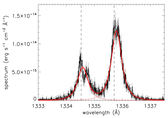
Optical depth effects, if present, are expected in chromospheric lines, because these atmospheric layers have densities higher than that of coronal structures. To check whether optical depth effects affect some chromospheric lines we inspected the Li-like and Na-like doublets of C IV (1548.19 and 1550.78 Å), N V (1238.82 and 1242.81 Å), and Si IV (1393.76 and 1402.77 Å). In the optically-thin collisionally-excited regime, the predicted ratio of the two lines of each doublet is 2:1. These ratios do not depend on temperature or abundances, and have a negligible dependence on interstellar absorption. Therefore the comparison between observed and predicted ratios can be performed irrespective of any source modeling.
The unabsorbed observed ratios of these three doublets are , , and , respectively. These values, slightly lower than those predicted, indicate that for the strongest lines of the inspected doublets, opacity effects are present but modest. This conclusion is further supported by the line profile observed in a few cases of strong UV lines. The clearest case is the profile of the two C II at Å (fig 13). Both the profiles clearly indicate a modest but clear line quenching near the peak. We exclude that this kind of line profile can be due to other effects, like for instance different velocity components, because, in that case, the same profile should characterize all the lines originating from the same plasma component. Notice however that measuring the fluxes of these lines using anyhow a single Gaussian encompassing the pairs of peaks, allows us to partially reconstruct the missing flux near the line peak.
In all cases (the inspected line doublets whose ratio marginally deviates from the optically-thin case, and the line profiles showing flux quenching) we are possibly underestimating the rate of emitted photons by a factor of . This factor is anyhow comparable with the uncertainties that characterize the derived EMD.
Appendix B V1298 Tau in comparison
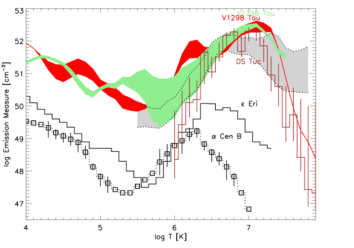
In order to put V1298 Tau in the wider context of coronal X-ray sources, in Fig. 14 we compare the Emission Measure Distribution (EMD) vs. temperature of V1298 Tau, derived with the two methods described in Sect. 4.3, with three other G–K stars with different activity levels and corresponding high-energy fluxes. In particular, we selected Cen B (K1V) as a prototype of a low-activity star (Sanz-Forcada et al., 2011), Eri (K2V) as an example of an intermediate-activity coronal source (Sanz-Forcada et al., 2003a), and DS Tuc A (G6V) as a high-activity object (Pillitteri et al., 2022). The latter is also a young planet-hosting star, about 40 Myr old, for which a study of the photo-evaporation of the planetary atmosphere was presented by Benatti et al. (2021), and strong flares were detected by XMM-Newton (Pillitteri et al., 2022), but we show just the EMD of the quiescent corona here for comparison.
The shift of the peak emission measure toward higher coronal temperatures, from MK to 10 MK for increasing activity level, was already noted by several authors in the past (see for example Scelsi et al. 2005). A similar trend is visible for the temperature of the minimum emission measures, but the variation is within a factor 3, from K to K. In the chromospheric region, from K to the temperatures at the minimum, the EMDs can be approximated with a power law, , with between 1.5 and 1.7, for all stars. This similarity was already assessed by Sanz-Forcada et al. (2011).
In the same figure, we show the EMD range predicted for very active stars according to Wood et al. (2018), who analyzed the X-ray spectra of 19 late-type dwarfs observed by Chandra, and showed a possible scaling of the EMDs with the surface X-ray flux. The coronal EMD of V1298 Tau, for temperatures above 1 MK, results in nice overlap with the range of values expected for stars having between 7.0 and 7.5 erg s-1 cm-2, i.e. those with the highest high-energy emission level in the study by Wood et al. (2018).
References
- Anders & Grevesse (1989) Anders, E., & Grevesse, N. 1989, Geochim. Cosmochim. Acta, 53, 197, doi: 10.1016/0016-7037(89)90286-X
- Arnaud (1996) Arnaud, K. A. 1996, in Astronomical Society of the Pacific Conference Series, Vol. 101, Astronomical Data Analysis Software and Systems V, ed. G. H. Jacoby & J. Barnes, 17
- Benatti et al. (2021) Benatti, S., Damasso, M., Borsa, F., et al. 2021, A&A, 650, A66, doi: 10.1051/0004-6361/202140416
- Bourrier et al. (2020) Bourrier, V., Wheatley, P. J., Lecavelier des Etangs, A., et al. 2020, MNRAS, 493, 559, doi: 10.1093/mnras/staa256
- Carleo et al. (2020) Carleo, I., Malavolta, L., Lanza, A. F., et al. 2020, A&A, 638, A5, doi: 10.1051/0004-6361/201937369
- Cecchi-Pestellini et al. (2006) Cecchi-Pestellini, C., Ciaravella, A., & Micela, G. 2006, A&A, 458, L13, doi: 10.1051/0004-6361:20066093
- Chadney et al. (2015) Chadney, J. M., Galand, M., Unruh, Y. C., Koskinen, T. T., & Sanz-Forcada, J. 2015, Icarus, 250, 357, doi: 10.1016/j.icarus.2014.12.012
- Coffaro et al. (2022) Coffaro, M., Stelzer, B., & Orlando, S. 2022, Astronomische Nachrichten, 343, e10066, doi: 10.1002/asna.20210066
- Coffaro et al. (2020) Coffaro, M., Stelzer, B., Orlando, S., et al. 2020, A&A, 636, A49, doi: 10.1051/0004-6361/201936479
- Cohen et al. (2014) Cohen, O., Drake, J. J., Glocer, A., et al. 2014, ApJ, 790, 57, doi: 10.1088/0004-637X/790/1/57
- Cosentino et al. (2014) Cosentino, R., Lovis, C., Pepe, F., et al. 2014, in Society of Photo-Optical Instrumentation Engineers (SPIE) Conference Series, Vol. 9147, Ground-based and Airborne Instrumentation for Astronomy V, ed. S. K. Ramsay, I. S. McLean, & H. Takami, 91478C, doi: 10.1117/12.2055813
- David et al. (2019) David, T. J., Petigura, E. A., Luger, R., et al. 2019, ApJ, 885, L12, doi: 10.3847/2041-8213/ab4c99
- Di Maio et al. (2020) Di Maio, C., Argiroffi, C., Micela, G., et al. 2020, A&A, 642, A53, doi: 10.1051/0004-6361/202038011
- Fitzpatrick (1999) Fitzpatrick, E. L. 1999, PASP, 111, 63, doi: 10.1086/316293
- Foster et al. (2012) Foster, A. R., Ji, L., Smith, R. K., & Brickhouse, N. S. 2012, ApJ, 756, 128, doi: 10.1088/0004-637X/756/2/128
- Fuhrmeister et al. (2022) Fuhrmeister, B., Czesla, S., Robrade, J., et al. 2022, A&A, 661, A24, doi: 10.1051/0004-6361/202141020
- Fulton & Petigura (2018) Fulton, B. J., & Petigura, E. A. 2018, AJ, 156, 264, doi: 10.3847/1538-3881/aae828
- Fulton et al. (2017) Fulton, B. J., Petigura, E. A., Howard, A. W., et al. 2017, AJ, 154, 109, doi: 10.3847/1538-3881/aa80eb
- Gabriel et al. (2004) Gabriel, C., Denby, M., Fyfe, D. J., et al. 2004, in Astronomical Society of the Pacific Conference Series, Vol. 314, Astronomical Data Analysis Software and Systems (ADASS) XIII, ed. F. Ochsenbein, M. G. Allen, & D. Egret, 759
- Gaia Collaboration (2020) Gaia Collaboration. 2020, VizieR Online Data Catalog, I/350
- Gomes da Silva et al. (2018) Gomes da Silva, J., Figueira, P., Santos, N., & Faria, J. 2018, The Journal of Open Source Software, 3, 667, doi: 10.21105/joss.00667
- Johnstone et al. (2021) Johnstone, C. P., Bartel, M., & Güdel, M. 2021, A&A, 649, A96, doi: 10.1051/0004-6361/202038407
- Kashyap & Drake (1998) Kashyap, V., & Drake, J. J. 1998, ApJ, 503, 450, doi: 10.1086/305964
- Khodachenko et al. (2007) Khodachenko, M. L., Ribas, I., Lammer, H., et al. 2007, Astrobiology, 7, 167, doi: 10.1089/ast.2006.0127
- King et al. (2018) King, G. W., Wheatley, P. J., Salz, M., et al. 2018, MNRAS, 478, 1193, doi: 10.1093/mnras/sty1110
- Lammer et al. (2003) Lammer, H., Selsis, F., Ribas, I., et al. 2003, ApJ, 598, L121, doi: 10.1086/380815
- Lammer et al. (2007) Lammer, H., Lichtenegger, H. I. M., Kulikov, Y. N., et al. 2007, Astrobiology, 7, 185, doi: 10.1089/ast.2006.0128
- Locci et al. (2019) Locci, D., Cecchi-Pestellini, C., & Micela, G. 2019, A&A, 624, A101, doi: 10.1051/0004-6361/201834491
- Lopez & Fortney (2013) Lopez, E. D., & Fortney, J. J. 2013, ApJ, 776, 2, doi: 10.1088/0004-637X/776/1/2
- Lovis et al. (2011) Lovis, C., Dumusque, X., Santos, N. C., et al. 2011, arXiv e-prints, arXiv:1107.5325. https://arxiv.org/abs/1107.5325
- Maggio et al. (2007) Maggio, A., Flaccomio, E., Favata, F., et al. 2007, ApJ, 660, 1462, doi: 10.1086/513088
- Maggio et al. (2022) Maggio, A., Locci, D., Pillitteri, I., et al. 2022, ApJ, 925, 172, doi: 10.3847/1538-4357/ac4040
- Mittag et al. (2013) Mittag, M., Schmitt, J. H. M. M., & Schröder, K. P. 2013, A&A, 549, A117, doi: 10.1051/0004-6361/201219868
- Oh et al. (2017) Oh, S., Price-Whelan, A. M., Hogg, D. W., Morton, T. D., & Spergel, D. N. 2017, AJ, 153, 257, doi: 10.3847/1538-3881/aa6ffd
- Owen & Lai (2018) Owen, J. E., & Lai, D. 2018, MNRAS, 479, 5012, doi: 10.1093/mnras/sty1760
- Owen & Wu (2013) Owen, J. E., & Wu, Y. 2013, ApJ, 775, 105, doi: 10.1088/0004-637X/775/2/105
- Owen & Wu (2017) —. 2017, ApJ, 847, 29, doi: 10.3847/1538-4357/aa890a
- Pillitteri et al. (2022) Pillitteri, I., Argiroffi, C., Maggio, A., et al. 2022, A&A, 666, A198, doi: 10.1051/0004-6361/202244268
- Pizzolato et al. (2003) Pizzolato, N., Maggio, A., Micela, G., Sciortino, S., & Ventura, P. 2003, A&A, 397, 147, doi: 10.1051/0004-6361:20021560
- Poppenhaeger et al. (2021) Poppenhaeger, K., Ketzer, L., & Mallonn, M. 2021, MNRAS, 500, 4560, doi: 10.1093/mnras/staa1462
- Raymond (1988) Raymond, J. C. 1988, in NATO ASIC Proc. 249: Hot Thin Plasmas in Astrophysics, ed. R. Pallavicini, 3+. http://adsabs.harvard.edu/cgi-bin/nph-bib_query?bibcode=1988htpa.conf....3R&db_key=AST
- Sanz-Forcada et al. (2003a) Sanz-Forcada, J., Brickhouse, N. S., & Dupree, A. K. 2003a, ApJS, 145, 147, doi: 10.1086/345815
- Sanz-Forcada et al. (2004) Sanz-Forcada, J., Favata, F., & Micela, G. 2004, A&A, 416, 281, doi: 10.1051/0004-6361:20034466
- Sanz-Forcada et al. (2022) Sanz-Forcada, J., López-Puertas, M., Nortmann, L., & Lampón, M. 2022, 21st Cambridge Workshop on Cool Stars, Stellar Systems, and the Sun, doi: 10.5281/zenodo.7561725
- Sanz-Forcada et al. (2003b) Sanz-Forcada, J., Maggio, A., & Micela, G. 2003b, A&A, 408, 1087, doi: 10.1051/0004-6361:20031025
- Sanz-Forcada et al. (2011) Sanz-Forcada, J., Micela, G., Ribas, I., et al. 2011, A&A, 532, A6, doi: 10.1051/0004-6361/201116594
- Scelsi et al. (2007) Scelsi, L., Maggio, A., Micela, G., Briggs, K., & Güdel, M. 2007, A&A, 473, 589, doi: 10.1051/0004-6361:20077792
- Scelsi et al. (2005) Scelsi, L., Maggio, A., Peres, G., & Pallavicini, R. 2005, A&A, 432, 671, doi: 10.1051/0004-6361:20041739
- Suarez Mascareño et al. (2021) Suarez Mascareño, A., Damasso, M., Lodieu, N., et al. 2021, Nature Astronomy, in press, doi: 10.1038/s41550-021-01533-7
- Suárez Mascareño et al. (2021) Suárez Mascareño, A., Damasso, M., Lodieu, N., et al. 2021, arXiv e-prints, arXiv:2111.09193. https://arxiv.org/abs/2111.09193
- Wargelin et al. (2017) Wargelin, B. J., Saar, S. H., Pojmański, G., Drake, J. J., & Kashyap, V. L. 2017, MNRAS, 464, 3281, doi: 10.1093/mnras/stw2570
- Wood et al. (2018) Wood, B. E., Laming, J. M., Warren, H. P., & Poppenhaeger, K. 2018, ApJ, 862, 66, doi: 10.3847/1538-4357/aaccf6