This paper has been submitted for publication in IEEE Transactions on Robotics.

This is the author’s version of an article that has, or will be, published in this journal or conference. Changes were, or will be, made to this version by the publisher prior to publication.

©2023  IEEE. Personal use of this material is permitted. Permission from IEEE must be obtained for all other uses, in any current or future media, including reprinting/republishing this material for advertising or promotional purposes, creating new collective works, for resale or redistribution to servers or lists, or reuse of any copyrighted component of this work in other works.

An Adaptive Graduated Nonconvexity Loss Function for Robust Nonlinear Least Squares Solutions

Abstract

Many problems in robotics, such as estimating the state from noisy sensor data or aligning two point clouds, can be posed and solved as least-squares problems. Unfortunately, vanilla nonminimal solvers for least-squares problems are notoriously sensitive to outliers. As such, various robust loss functions have been proposed to reduce the sensitivity to outliers. Examples of loss functions include pseudo-Huber, Cauchy, and Geman-McClure. Recently, these loss functions have been generalized into a single loss function that enables the best loss function to be found adaptively based on the distribution of the residuals. However, even with the generalized robust loss function, most nonminimal solvers can only be solved locally given a prior state estimate due to the nonconvexity of the problem. The first contribution of this paper is to combine graduated nonconvexity (GNC) with the generalized robust loss function to solve least-squares problems without a prior state estimate and without the need to specify a loss function. Moreover, existing loss functions, including the generalized loss function, are based on Gaussian-like distribution. However, residuals are often defined as the squared norm of a multivariate error and distributed in a Chi-like fashion. The second contribution of this paper is to apply a norm-aware adaptive robust loss function within a GNC framework. The proposed approach enables a GNC formulation of a generalized loss function such that GNC can be readily applied to a wider family of loss functions. Furthermore, simulations and experiments demonstrate that the proposed method is more robust compared to non-GNC counterparts, and yields faster convergence times compared to other GNC formulations.

I Introduction

Least squares problems appear in robotics, computer vision, and data analytics. However, traditional least-squares solvers perform poorly in the presence of outliers that are often caused by spurious sensor data [Roysdon2017], faulty data association [Neira2001], and model misspecification [1]. To reduce the sensitivity to outliers during minimization of a least-squares objective function, robust loss functions (RLFs) [DeMenezes2021], such as pseudo-Huber [2], Cauchy [3], and Geman-McClure [4], have been proposed. However, the main drawback of these RLFs is that they must be hand-picked and manually tuned a priori without knowledge of the actual residual distribution.

I-A Prior Work

A generalized loss function capable of adapting to the actual residual distribution was presented in [5], where it was shown to represent a superset of many common RLFs. A single continuous-valued hyperparameter in the loss function can be set such that the function is adjusted to model a wider family of problems with improve flexibility. The adaptive loss function in [5] was originally implemented in computer vision tasks. Later, [5] was extended and applied to general nonlinear least-squares problems in [6] by incorporating the hyperparameter as a part of the estimation process. Also, [6] extended the usable range of this parameter to deal with a larger set of outlier distributions.

Recently, [7] noted that most of the loss functions assume the residuals follow a Gaussian-like distribution with a mode of zero. However, in most nonlinear least-squares problems, the residuals are defined as the norm of a multivariate error, which results in a Chi-like distribution with a nonzero mode. Thus, applying the adaptive loss function directly to the residual distribution may lead to poor weight assignment. This issue was addressed in [7] by finding the mode of the Chi-like distribution and applying the adaptive loss function to the mode-shifted residuals. The proposed method, called the adaptive Maxwell-Boltzmann (AMB), was demonstrated in point-cloud alignment and pose averaging, and outperformed other state-of-the-art RLFs.

Nonlinear least-squares problems are difficult to solve globally due to the nonconvexity of the objective function [8]. Furthermore, [8] indicated that most of the nonminimal solvers are only able to obtain locally optimal solutions. To address this problem, [8] proposed to combine nonminimal solvers with a method known as graduated nonconvexity (GNC) [9] to solve optimization problems without requiring an initial estimate. GNC and the Black-Rangarajan duality [9] were tailored to traditional loss functions like Geman-McClure (GM) and truncated least-squares (TLS), and used with nonminimal solvers in point-cloud registration, mesh registration, pose-graph optimization, and shape alignment. Although GNC’s global optimality cannot be guaranteed, the proposed method was able to solve the aforementioned problems without requiring an initial guess of the state prior to optimization, resulting in a more accurate solution compared to other local solvers.

I-B Statement of Contribution

The primary contribution of this work is a detailed derivation of the adaptive loss function and GNC combination (AGNC). Previously, GNC has been tailored to a specific loss function of choice. However, the combination of GNC with the generalized loss function no longer necessitates the specification of a particular loss function and shows more robustness even with a highly nonconvex objective function. The idea of blending GNC with the generalized loss function is mentioned in [5]. However, the specific derivation, nor its limitations, are discussed.

The secondary contribution of this paper is to acknowledge the Chi-like residual distribution and incorporate GNC into AMB (GNC AMB). Accounting for the mode of the residual distribution is expected to deliver faster convergence rates and more robust performance than AGNC. The proposed method is tested against fixed RLFs, adaptive RLFs, and other GNC-incorporated loss functions.

I-C Paper Organization

The remainder of this paper is organized as follows. Section II reviews concepts such as standard and adaptive RLFs, GNC, and AMB. Section III presents the derivation of the novel AGNC loss function. The proposed methods are applied to a linear regression, a point-cloud alignment, and a mesh registration problem in Section IV. Finally, the paper is drawn to a close in Section V.

II Preliminaries

Let ${\mbf{e}_{i}=\mbf{e}(\mbf{y}_{i},\mbf{g}(\mbf{x}))}$ be an error function that quantifies the difference between the ${i}$-th measurement ${\mbf{y}_{i}}$ and the expected measurement given a measurement model ${\mbf{g}(\cdot)}$ and a state ${\mbf{x}}$. The Mahalanobis distance of the error function is

$$\epsilon_{i}\left(\mbf{y}_{i},\mbf{x}\right) =\left\|\mbf{e}_{i}\right\|_{\bm{\Sigma}_{i}^{-1}}=\sqrt{\mbf{e}_{i}^{{\mathsf{T}}}\bm{\Sigma}_{i}^{-1}\mbf{e}_{i}},$$ (1)

where ${\bm{\Sigma}_{i}}$ is the covariance on the ${i}$-th error. For brevity of notation, ${\epsilon_{i}=\epsilon_{i}\left(\mbf{y}_{i},\mbf{x}\right)}$.

II-A Robust Loss Functions

Consider the following least-squares problem,

$$\mbf{x}^{\star} =\underset{\mbf{x}\in\mathcal{X}}{\operatorname*{arg\,min}}\sum_{i=1}^{N}\mbox{$\textstyle{\frac{1}{2}}$}\epsilon_{i}^{2},$$ (2)

where ${\mbf{x}\in\mathcal{X}}$ is the state to be estimated and ${N}$ is the number of measurements. In the presence of outliers, (2) provides a poor estimate of ${\mbf{x}}$. Robust least-squares solvers substitute the quadratic cost in (2) with a loss function ${\rho(\cdot)}$,

$$\mbf{x}^{\star} =\underset{\mbf{x}\in\mathcal{X}}{\operatorname*{arg\,min}}\sum_{i=1}^{N}\rho\left(\epsilon_{i}\right).$$ (3)

Equation 3 can be solved using an iteratively reweighted least-squares (IRLS) framework [10] that solves a sequence of weighted least-squares problems,

$$\mbf{x}^{\star} =\underset{\mbf{x}\in\mathcal{X}}{\operatorname*{arg\,min}}\sum_{i=1}^{N}\mbox{$\textstyle{\frac{1}{2}}$}w_{i}\epsilon_{i}^{2}.$$ (4)

The weights ${w_{i}}$ in (4) are obtained by equating the gradients of the loss function in (3) and (4) with respect to ${\mbf{x}}$,

$$\frac{\partial\rho\left(\epsilon_{i}\right)}{\partial\epsilon_{i}}\frac{\partial\epsilon_{i}}{\partial\mbf{x}} =w_{i}\epsilon_{i}\frac{\partial\epsilon_{i}}{\partial\mbf{x}},$$ (5a)

$$w_{i} =\frac{1}{\epsilon_{i}}\frac{\partial\rho\left(\epsilon_{i}\right)}{\partial\epsilon_{i}}.$$ (5b)

This approach allows standard solvers like Gauss-Newton and Levenberg-Marquardt algorithms to solve (3).

II-B Black-Rangarajan Duality and Graduated Nonconvexity

The Black-Rangarajan duality introduces regularization in (3),

$$\mbf{x}^{\star},\mbf{w}^{\star} =\underset{\mbf{x}\in\mathcal{X},w_{i}\in(0,1]}{\operatorname*{arg\,min}}\sum_{i=1}^{N}\left(\mbox{$\textstyle{\frac{1}{2}}$}w_{i}\epsilon_{i}^{2}+\Phi_{\rho}\left(w_{i}\right)\right),$$ (6)

where ${w_{i}}$ is the weight associated to ${i}$-th measurement, ${\mbf{w}^{\star}}$ is the vector form of optimal weights, and the outlier process function ${\Phi_{\rho}(\cdot)}$ defines a penalty on ${w_{i}}$ [9]. An appropriate regularization function ${\Phi_{\rho}(\cdot)}$ must be found for a particular loss function ${\rho(\cdot)}$.

Lemma II.1 (Black-Rangarajan Duality).

Given a loss function ${\rho(\cdot)}$, define ${\phi(z)\coloneqq\rho(\sqrt{z})}$. If ${\phi(z)}$ satisfies

$$\lim_{z\to{0}}\phi^{\prime}(z) =\mbox{$\textstyle{\frac{1}{2}}$},$$ (7a)

$$\lim_{z\to{\infty}}\phi^{\prime}(z) =0,$$ (7b)

$$\phi^{\prime\prime}(z) <0,$$ (7c)

then there exists an analytical outlier process function ${\Phi_{\rho}(\cdot)}$ that can be written as

$$\rho\left(\epsilon\right) =\mbox{$\textstyle{\frac{1}{2}}$}w\epsilon^{2}+\Phi_{\rho}\left(w\right).$$ (8)

The analytical expression of ${\Phi_{\rho}(\cdot)}$ is derived in the Appendix A.

The conditions on ${\rho(\cdot)}$ are satisfied by all common choices of robust loss functions [9]. This duality converts (3) into polynomials by regularizing (4) with an additional constraint ${\Phi_{\rho}(\cdot)}$, and also provides an analytical expression for ${\Phi_{\rho}(\cdot)}$. However, the duality does not enable solving a highly nonconvex optimization problem with poor initial estimates. This nonconvexity can be tackled by using GNC [11].

The idea behind GNC is to choose a surrogate function ${\rho_{\mu}(\cdot)}$ with a control parameter ${\mu}$ that changes the shape of ${\rho(\cdot)}$ such that (6) can be rewritten as

$$\mbf{x}^{\star},\mbf{w}^{\star} =\underset{\mbf{x}\in\mathcal{X},w_{i}\in(0,1]}{\operatorname*{arg\,min}}\sum_{i=1}^{N}\left(\mbox{$\textstyle{\frac{1}{2}}$}w_{i}\epsilon_{i}^{2}+\Phi_{\rho_{\mu}}\left(w_{i}\right)\right),$$ (9)

where ${\Phi_{\rho_{\mu}}(\cdot)}$ is the outlier process function for the surrogate RLF, ${\rho_{\mu}(\cdot)}$. The parameter ${\mu}$ allows a convex approximation of ${\rho(\cdot)}$ to be obtained such that it can be readily minimized. GNC solves the nonconvex problem by gradually increasing the nonconvexity of ${\rho_{\mu}(\cdot)}$ during optimization until it recovers the original function. In [8], (9) is solved using IRLS by modifying ${\mu}$ at every iteration.

II-C Adaptive Robust Loss

This section discusses the formulation of the adaptive loss function proposed in [5], its limitations, and the solutions to the limitations proposed by [6]. The simplest form of the adaptive loss function is

$$\rho\left(\epsilon,\alpha\right) =\frac{\left|\alpha-2\right|}{\alpha}\left(\left(\frac{\epsilon^{2}}{\left|\alpha-2\right|}+1\right)^{\nicefrac{{\alpha}}{{2}}}-1\right),$$ (10)

where ${\alpha\in(-\infty,2]}$ is a shape parameter that controls the robustness of the loss. Accounting for singularities, (10) is rewritten in a piecewise function as

$$\rho\left(\epsilon,\alpha\right) =\begin{cases}\mbox{$\textstyle{\frac{1}{2}}$}\epsilon^{2}&\textrm{if }\alpha=2,\\ \log\left(\mbox{$\textstyle{\frac{1}{2}}$}\epsilon^{2}+1\right)&\textrm{if }\alpha=0,\\ 1-\exp\left(-\mbox{$\textstyle{\frac{1}{2}}$}\epsilon^{2}\right)&\textrm{if }\alpha=-\infty,\\ \frac{\left|\alpha-2\right|}{\alpha}\left(\left(\frac{\epsilon^{2}}{\left|\alpha-2\right|}+1\right)^{\nicefrac{{\alpha}}{{2}}}-1\right)&\textrm{otherwise}.\end{cases}$$ (11)

In [5], ${\alpha}$ is treated as an additional unknown parameter to be optimized along with ${\mbf{x}}$ in the generalized loss function,

$$\mbf{x}^{\star},\alpha^{\star} =\underset{\mbf{x}\in\mathcal{X},\alpha\in(-\infty,2]}{\operatorname*{arg\,min}}\sum_{i=1}^{N}\rho\left(\epsilon_{i},\alpha\right).$$ (12)

However, naively solving for (12) can result in a trivial solution with some ${{\alpha}^{\star}}$ that downweights all the residuals without affecting ${\mbf{x}}$. Thus, [5] avoids this by adding a regularization term derived from the probability distribution,

$$p\left(\epsilon|\mu_{\epsilon},\alpha\right) =\frac{1}{Z\left(\alpha\right)}\exp\left(-\rho\left(\epsilon-\mu_{\epsilon},\alpha\right)\right),$$ (13a)

$$Z\left(\alpha\right) =\int_{-\infty}^{\infty}\exp\left(-\rho\left(\epsilon|\mu_{\epsilon},\alpha\right)\right)\mathrm{d}\epsilon,$$ (13b)

where ${\mu_{\epsilon}}$ is the residual mean and ${Z(\alpha)}$ is a partition function. The general adaptive loss with the regularization term is constructed from the negative log-likelihood of (13a),

$$\rho_{a}\left(\epsilon,\alpha\right) =-\log\left(p\left(\epsilon|\mu_{\epsilon},\alpha\right)\right)$$ (14a)

$$=\rho\left(\epsilon,\alpha\right)+\log\left(Z\left(\alpha\right)\right).$$ (14b)

However, (14b) is only defined for ${\alpha\geq 0}$ because ${Z(\alpha)}$ diverges when ${\alpha<0}$.

To solve this issue, [6] computes an approximate partition function ${\tilde{Z}(\alpha)}$ by limiting the integral bounds with a hyperparameter ${\tau}$ such that

$$\tilde{Z}\left(\alpha\right) =\int_{-\tau}^{\tau}\exp\left(-\rho\left(\epsilon|\mu_{\epsilon},\alpha\right)\right)\mathrm{d}\epsilon.$$ (15)

This allows the shape parameter to be dynamically adapted for values between ${-\infty}$ and ${2}$. The truncation bound is often set for a specific problem. For example, if the magnitude of the residuals is expected to be large, a larger ${\tau}$ value is used. Further, [6] finds the optimal shape parameter through a grid search by solving the optimization problem

$$\alpha^{\star} =\underset{\alpha\in(-\infty,2]}{\operatorname*{arg\,min}}-\log\left(p\left(\epsilon|\mu_{\epsilon}\alpha\right)\right)$$ (16a)

$$=\underset{\alpha\in(-\infty,2]}{\operatorname*{arg\,min}}N\log\left(\tilde{Z}\left(\alpha\right)\right)+\sum_{i=1}^{N}\rho\left(\epsilon_{i},\alpha\right).$$ (16b)

Having ${{\alpha}^{\star}}$ and the loss function (14b), the weights ${w_{i}}$ are obtained using (5b),

$$w\left(\epsilon,\alpha^{\star}\right) =\begin{cases}1&\textrm{if }\alpha^{\star}=2,\\ \frac{2}{\epsilon^{2}+2}&\textrm{if }\alpha^{\star}=0,\\ \exp\left(-\mbox{$\textstyle{\frac{1}{2}}$}\epsilon^{2}\right)&\textrm{if }\alpha^{\star}=-\infty,\\ \left(\frac{\epsilon^{2}}{\left|\alpha^{\star}-2\right|}+1\right)^{\nicefrac{{\alpha^{\star}}}{{2}}-1}&\textrm{otherwise}.\end{cases}$$ (17)

II-D Adaptive Maxwell-Boltzmann Loss

Residuals are often defined as a squared norm of a multivariate error that follows a Chi distribution with some nonzero peak, ${\tilde{\epsilon}}$. However, most of the existing RLFs are derived based on Gaussian-like distribution with its peak at zero. Therefore, the residuals will be weighted the highest near zero and weighted less as they get further away from zero. Recently, [7] discovered that this Gaussian assumption results in lower weights assigned to residuals clustered around the non-zero mode value. As such, [7] proposed the AMB loss function that addresses this problem by first fitting an ${n_{e}}$-dimensional Maxwell-Boltzmann (MB) distribution to the residuals,

$$p_{\textrm{MB}}\left(\epsilon|a,n_{e}\right) =\frac{\epsilon^{n_{e}-1}}{a^{n_{e}}2^{\left(\nicefrac{{n_{e}}}{{2}}-1\right)}\Gamma\left(\nicefrac{{n_{e}}}{{2}}\right)}\exp\left(-\nicefrac{{\epsilon^{2}}}{{2a^{2}}}\right),$$ (18)

where ${n_{e}}$ is the dimension of the residual and ${a}$ is the MB shape parameter. The optimal shape parameter ${a^{\star}}$ can be found by minimizing the negative log-likelihood of (18) with respect to ${a}$. However, this could result in poor estimation in the presence of outliers. Thus, ${a^{\star}}$ is found by solving

$$a^{\star} =\underset{a\in\mathbb{R}^{+}}{\operatorname*{arg\,min}}\int_{0}^{\tau}\left(q\left(\epsilon\right)\cdot\left(p_{\textrm{MB}}\left(\epsilon|a,n_{e}\right)-q\left(\epsilon\right)\right)\right)^{2}\mathrm{d}\epsilon,$$ (19)

where ${q(\epsilon)}$ is the residual distribution. This results in a better fit in high-frequency inlier areas. Equation (19) is solved analytically using Newton’s method with a line search [7]. The optimal shape parameter is used to find the nonzero mode value,

$$\tilde{\epsilon} =a^{\star}\sqrt{n_{e}-1}.$$ (20)

Residuals satisfying ${\epsilon\leq\tilde{\epsilon}}$ are considered inliers and assigned a weight equal to ${1}$, and any residuals satisfying ${\epsilon>\tilde{\epsilon}}$ are assigned a weight that is strictly less than one in an adaptive fashion. To do so, the optimal shape parameter ${\alpha^{\star}}$ that fits the mode-shifted residuals, ${\xi=\epsilon-\tilde{\epsilon}}$, is computed using (16b)

$$\alpha^{\star}=\underset{\alpha\in(-\infty,2]}{\operatorname*{arg\,min}}M\log\left(\tilde{Z}\left(\alpha\right)\right)+\sum_{i=1}^{M}\rho\left(\xi_{i},\alpha\right),$$ (21)

where ${M}$ is the total number of ${\xi_{i}}$. The partition function ${\tilde{Z}(\cdot)}$ is now computed with the mode-shifted truncation bound, ${\tilde{\tau}=\tau-\tilde{\epsilon}}$,

$$\tilde{Z}\left(\alpha\right)=\int_{0}^{\tilde{\tau}}\exp\left(-\rho\left(\xi|\mu_{\xi},\alpha\right)\right)\mathrm{d}\xi.$$ (22)

Thus, given ${\tilde{\epsilon}}$ and ${\alpha^{\star}}$, the weights are

$$\tilde{w}\left(\epsilon,\tilde{\epsilon},\alpha^{\star}\right) =\begin{cases}1&\textrm{if }\epsilon\leq\tilde{\epsilon},\\ w\left(\epsilon-\tilde{\epsilon},\alpha^{\star}\right)&\textrm{if }\epsilon>\tilde{\epsilon}.\end{cases}$$ (23)

These weights ${w(\cdot)}$ in (23) are from (17). A detailed derivation and visualization of the AMB loss function ${\rho(\epsilon,\tilde{\epsilon},\alpha)}$ can be found in Appendix B.

III Methodology

This section first presents the derivation of the proposed adaptive graduated nonconvexity (AGNC) loss function. Assuming that the optimal shape parameter ${\alpha^{\star}}$ is precomputed using (16b), GNC is incorporated into (10). Based on the properties inherited from GNC, optimization with the proposed loss function is expected to converge without any prior state estimate. Further, the proposed method is extended to adapt the nonzero peak of the residual distribution by incorporating AMB from [7].

III-A GNC Surrogate Function to Adaptive Robust Loss

Suppose there exists a surrogate function of (10) of the form

$$\rho_{\mu}\left(\epsilon,\alpha^{\star}\right) =\frac{\left|f-2\right|}{f}\left(\left(\frac{\epsilon^{2}}{\left|f-2\right|}+1\right)^{\nicefrac{{f}}{{2}}}-1\right),$$ (24)

where ${f=f(\mu,\alpha^{\star})}$ is a shape function that takes in the optimal shape parameter ${\alpha^{\star}}$ and the convexity control parameter ${\mu}$ as inputs to determine the shape of the adaptive loss function. Recall that GNC computes a solution to the nonconvex problem by starting from its convex surrogate and gradually increasing its nonconvexity until the original function is recovered. Notice that ${\rho_{\mu}(\cdot)}$ becomes quadratic in the limit of ${f(\cdot)\to 2}$, and that ${\rho(\cdot)}$ is recovered in the limit of ${f(\cdot)\to\alpha^{\star}}$. Also, ${f(\cdot)\leq{2}}$ for all ${\mu}$ because (10) is only defined for ${\alpha\in(-\infty,2]}$. As such, the shape function ${f(\cdot)}$ must satisfy the conditions,

$$\lim_{\mu\to{c_{1}}}f\left(\mu,\alpha^{\star}\right) =2,$$ (25a)

$$\lim_{\mu\to{c_{2}}}f\left(\mu,\alpha^{\star}\right) =\alpha^{\star},$$ (25b)

$$f\left(\mu,\alpha^{\star}\right)\leq 2.$$ (25c)

The parameters ${c_{1}}$ and ${c_{2}}$ are user-defined constants. The choice of ${c_{1}}$ and ${c_{2}}$ determines the shape of ${f(\cdot)}$, which governs the amount of nonconvexity added to the convex surrogate at each iteration. Thus, the convergence rate of the AGNC loss function depends on the choice of ${f(\cdot)}$. Some examples of the shape functions depending on the choice of ${c_{1}}$ and ${c_{2}}$ are presented next.

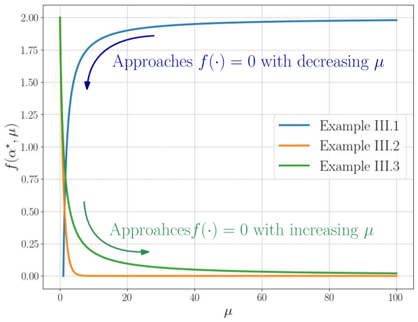
Figure 1: Shape functions with ${\alpha^{\star}=0}$ for Examples III.1, III.2, and III.3 shown in blue, orange, and green lines, respectively. Blue line approaches ${f(\cdot)=\alpha^{\star}}$ as ${\mu}$ decreases towards ${1}$, whereas orange and green lines approach ${f(\cdot)=\alpha^{\star}}$ as ${\mu}$ increases towards ${\infty}$. However, the rate at which ${f(\cdot)}$ approaches ${\alpha^{\star}}$, also interpreted as the amount of nonconvexity added to the surrogate loss function ${\rho_{\mu}(\cdot)}$, is higher in the orange line (Example III.2).

Example III.1.

Let ${c_{1}=\infty}$ and ${c_{2}=1}$ such that the original function is restored as ${\mu}$ decreases from ${\infty}$ to ${1}$. Amongst others, the shape function ${f(\cdot)}$ can be formulated as

$$f\left(\mu,\alpha^{\star}\right) =\frac{\alpha^{\star}+2\mu-2}{\mu},$$ (26)

such that

$$\lim_{\mu\to{\infty}}f\left(\mu,\alpha^{\star}\right) =\lim_{\mu\to{\infty}}\frac{\alpha^{\star}+2\mu-2}{\mu}=2,$$ (27a)

$$\lim_{\mu\to{1}}f\left(\mu,\alpha^{\star}\right) =\lim_{\mu\to{1}}\frac{\alpha^{\star}+2\mu-2}{\mu}=\alpha^{\star},$$ (27b)

$$f\left(\mu,\alpha^{\star}\right) \leq 2,\ \forall\mu\in[1,\infty).$$ (27c)

However, when ${\alpha^{\star}=-\infty}$, (27a) and (27b) are undefined. As such, another shape function is used for ${\alpha^{\star}=-\infty}$,

$$f\left(\mu,\alpha\right) =f\left(\mu\right)=\frac{2\mu-3}{\mu-1},$$ (28)

which satisfies

$$\lim_{\mu\to{\infty}}f\left(\mu\right) =2,$$ (29a)

$$\lim_{\mu\to{1^{+}}}f\left(\mu\right) =-\infty.$$ (29b)

In practice, the convexity control parameter ${\mu}$ decreases from some initial value ${\mu_{0}=\max\left(\epsilon^{2}\right)}$ to ${1}$ by

$$\mu_{k}=\left(\mu_{k-1}-1\right)/c+1,$$ (30)

where ${c}$ is some constant.

Example III.2.

Alternatively, let ${c_{1}=0}$ and ${c_{2}=\infty}$ to represent increasing ${\mu}$. Then, the shape function ${f(\cdot)}$ can be formulated as

$$f\left(\mu,\alpha^{\star}\right) =\alpha^{\star}\exp\left(\frac{1}{-\mu}\right)+2\exp\left(-\mu\right),$$ (31)

such that

$$\lim_{\mu\to{0^{+}}}f\left(\mu,\alpha^{\star}\right) =\lim_{\mu\to{0^{+}}}\alpha^{\star}\exp\left(\frac{1}{-\mu}\right)+2\exp\left(-\mu\right)=2,$$ (32a)

$$\lim_{\mu\to{\infty}}f\left(\mu,\alpha^{\star}\right) =\lim_{\mu\to{\infty}}\alpha^{\star}\exp\left(\frac{1}{-\mu}\right)+2\exp\left(-\mu\right)=\alpha^{\star},$$ (32b)

$$f\left(\mu,\alpha^{\star}\right) \leq 2,\ \forall\mu\in\mathbb{R}^{+}.$$ (32c)

Again, for ${\alpha^{\star}=-\infty}$, (32a) and (32a) are not satisfied. Thus, a different shape function is chosen for this edge case,

$$f\left(\mu,\alpha^{\star}\right) =f\left(\mu\right)=2-\mu,$$ (33)

which satisfies

$$\lim_{\mu\to{0^{+}}}f\left(\mu\right) =\lim_{\mu\to{0^{+}}}2-\mu=2,$$ (34a)

$$\lim_{\mu\to{\infty}}f\left(\mu\right) =\lim_{\mu\to{\infty}}2-\mu=-\infty.$$ (34b)

With this shape function, the convexity parameter ${\mu}$ increases from some initial value ${\mu_{0}=\frac{1}{\max\left(\epsilon^{2}\right)}}$ to ${\infty}$ by

$$\mu_{k}=c\mu_{k-1},$$ (35)

where ${c}$ is some constant.

Example III.3.

With the same choice of the constants as in Example III.2, a different shape function ${f(\cdot)}$ can be formulated as

$$f\left(\mu,\alpha^{\star}\right) =\frac{\alpha^{\star}\mu+2}{\mu+1},$$ (36)

such that

$$\lim_{\mu\to{0}^{+}}f\left(\mu,\alpha^{\star}\right) =\lim_{\mu\to{0}^{+}}\frac{\alpha^{\star}\mu+2}{\mu+1}=2,$$ (37)

$$\lim_{\mu\to\infty}f\left(\mu,\alpha^{\star}\right) =\lim_{\mu\to{\infty}}\frac{\alpha^{\star}\mu+2}{\mu+1}=\alpha^{\star},$$ (38)

$$f\left(\mu,\alpha^{\star}\right) \leq 2,\ \forall\mu\in\mathbb{R}^{+}.$$ (39)

Despite having the same ${c_{1}}$ and ${c_{2}}$ for both Example III.2 and Example III.3, their shape functions behave differently as shown in Figure 1. The shape function in Example III.2, represented by the orange line, approaches ${f(\cdot)=\alpha^{\star}}$ faster than the one in Example III.3, represented by the green line, which may lead to a faster convergence at the expense of robustness of the solver. However, a detailed analysis as to what what shape function to use is not provided. As such, the shape function is left as a user-defined function.

Algorithm 1 Implementation of AGNC

${\bm{\epsilon}=\begin{bmatrix}\epsilon_{1}&\epsilon_{2}&\ldots&\epsilon_{N}\end{bmatrix}^{{\mathsf{T}}}}$, ${\mu}$

${\epsilon_{i}=\left\|\mbf{e}_{i}\right\|_{\Sigma^{-1}}}$

Select ${\alpha^{\star}}$ or compute using (16b).

Select a shape function ${f(\mu,\alpha^{\star})}$

Select an initial convexity parameter ${\mu|f(\mu,\alpha^{\star})\to 2}$

while $f\neq\alpha^{\star}$ do

     Compute ${f(\mu,\alpha^{\star})}$.

     Compute the optimal weights ${\mbf{w}^{\star}}$ for ${\bm{\epsilon}}$ using (41).

     Solve for the states ${\mbf{x}^{\star}}$ with ${\mbf{w}^{\star}}$ using (4).

     Update ${\mu}$ such that ${f(\mu,\alpha^{\star})}$ approaches $\alpha^{\star}$.

end while

Algorithm 2 Implementation of GNC on AMB

${\bm{\epsilon}=\begin{bmatrix}\epsilon_{1}&\epsilon_{2}&\ldots&\epsilon_{N}\end{bmatrix}^{{\mathsf{T}}}}$, ${\mu}$

${\epsilon_{i}=\left\|\mbf{e}_{i}\right\|_{\Sigma^{-1}}}$

Compute ${a^{\star}}$ of ${q(\bm{\epsilon})}$ using (19).

Compute ${\tilde{\epsilon}}$ using (20).

Compute the mode-shifted values

$$\bm{\xi}=\bm{\epsilon}-\tilde{\epsilon}\mathbbm{1}\textrm{ and }\tilde{\tau}=\tau-\tilde{\epsilon},$$

where ${\mathbbm{1}}$ is a column matrix of ones.

Compute ${\alpha^{\star}}$ of ${q(\bm{\xi})}$ using (21) and (22).

Perform Algorithm 1 on ${\bm{\xi}}$ with ${\alpha^{\star}}$.

TABLE I: Abbreviations used for different loss functions.

Abbreviation	Method	Description
C	Cauchy	[3]
W	Welsch	[12]
GM	Geman-McClure	[4]
TLS	Truncated least squares	[8]
BA	Adaptive loss	[5]
CA	Adaptive loss	[6]
AMB	Adaptive MB	[7]
G-C	GNC-Cauchy	GNC with to Cauhcy
G-W	GNC-Welsch	GNC with to Welsch
G-GM	GNC-GM	GNC with to GM
G-TLS	GNC-TLS	[8]
G-${\alpha^{\star}}$	GNC-${\alpha^{\star}}$	GNC with to adaptive loss with ${\alpha^{\star}}$ from (16b)
G-AMB	GNC-AMB	GNC with to Adaptive MB

III-B Adaptive GNC Weight Update

Similar to [8], (9) is optimized using IRLS with changing ${\mu}$. The states ${\mbf{x}}$ and the weights ${w_{i}}$ are optimized alternatively and iteratively. Recall that the Mahalanobis distance of the residual is a function of ${\mbf{x}}$. Thus, minimizing (9) with respect to ${\mbf{x}}$ and fixed weights ${w_{i}}$ results in minimizing (4) because the outlier process function does not depend on ${\mbf{x}}$. On the other hand, minimizing (9) with respect to ${w_{i}}$ and fixed ${\bar{\mbf{x}}}$ results in

$$\mbf{w}^{\star}=\underset{w_{i}\in(0,1]}{\operatorname*{arg\,min}}\sum_{i=1}^{N}\mbox{$\textstyle{\frac{1}{2}}$}w_{i}\epsilon_{i}\left(\bar{\mbf{x}}\right)^{2}+\Phi_{\rho_{\mu}}\left(w_{i}\right).$$ (40)

With ${\Phi_{\rho_{\mu}}(\cdot)}$ derived in Appendix C, the solution to (40) for changing values of ${\mu}$ is given as

$$w^{\star}\left(\epsilon,\alpha^{\star}\right) =\begin{cases}1&\textrm{if }f=2,\\ \frac{2}{\epsilon^{2}+2}&\textrm{if }f=0,\\ \exp\left(-\mbox{$\textstyle{\frac{1}{2}}$}\epsilon^{2}\right)&\textrm{if }f=-\infty,\\ \left(\frac{\epsilon^{2}}{\left|f-2\right|}+1\right)^{\nicefrac{{f}}{{2}}-1}&\textrm{otherwise}.\end{cases}$$ (41)

Implementation of AGNC is shown in Algorithm 1.

III-C GNC Algorithm with AMB Loss

Recall that most of the robust loss functions that are subsets of (10) assume a Gaussian-like residual distribution, and this assumption can inadvertently lead to problems with the weighting scheme [7]. Thus, the adaptive GNC loss function is extended to incorporate the “mode gap” approach of [7].

The mode of the residual distribution ${\tilde{\epsilon}}$ is estimated using (20) by fitting an MB distribution (18) to the residual distribution ${q(\epsilon)}$ as shown in (19). Having estimated the mode value, the optimal shape parameter for the mode-shifted residuals is found using (21) and (22). With a fixed ${a^{\star}}$, GNC is applied to the AMB loss function. Implementation of GNC on AMB (GNC-AMB) is shown in Algorithm 2.

IV Results

The proposed AGNC algorithm is tailored to 5 RLFs, Cauchy [3], Welsch [12], Geman-McClure [4], Barron’s adaptive robust loss [5], and Hitchcox and Forbes’ adaptive MB [7], for their good performance in a similar study [13, 7]. The GNC variants of these loss functions, denoted as GNC-Cauchy, GNC-Welsch, GNC-GM, GNC-${\alpha^{\star}}$, and GNC-AMB, respectively, are derived using the methodology described in Section III and compared against their baseline loss functions as well as Chebrolu et al.’s adaptive robust loss [6]. Also, the proposed methods are compared against existing GNC-applied loss functions like GNC with Geman-McClure and GNC with truncated least-squares from [8]. Abbreviations of these loss functions are shown in Table I. The proposed methods are tested on a variety of problems including the simple multidimensional linear regression problem from [8], a point-cloud alignment problem, and a mesh registration problem.

TABLE II: Performance of the loss functions in the linear regression problem. Median errors and processing times are shown for various loss functions and their corresponding GNC variants. Middle column of Geman-McClure is the GNC-incorporated Geman McClure loss function proposed by [8]. The errors are scaled by a $1\text{\times}{10}^{3}\text{\,}$ for readability. For each loss function, the best performance between the traditional and adaptive formulations is highlighted in each row. The lowest error for each outlier level is highlighted in blue.

	% outliers	Cauchy	G-C	Welsch	G-W	GM	G-GM [8]	G-GM	BA	CA	AGNC	AMB	G-AMB
Median Error	20%	8.65	3.81	14.4	4.15	10.7	4.09	4.09	8.65	9.07	3.84	4.04	3.91
	40%	11.4	5.06	17.0	4.43	13.3	5.54	5.54	11.4	12.3	5.24	4.97	4.81
	60%	12.6	5.50	22.4	5.90	15.7	6.11	6.11	12.6	14.8	6.15	6.26	6.12
	80%	17.4	7.50	23.0	12.4	18.0	8.10	8.10	17.4	19.3	9.17	10.6	10.0
Time (s)	ALL	0.005	0.130	0.006	0.622	0.005	0.466	0.138	0.023	0.021	0.166	0.019	0.149

TABLE III: Linear regression problem results of the proposed GNC-AMB and AGNC loss function with various ${\alpha^{\star}}$ are compared against GNC-TLS. Error percentiles are shown in different outlier levels, and mean processing time and median number of iterations to converge are shown for all outlier levels. The errors are scaled by a $1\text{\times}{10}^{3}\text{\,}$ for readability. The lowest error in each percentile as well as the lowest time and the number of iterations are highlighted in bold.

	% outliers	GNC-TLS	GNC-Cauchy	GNC-Welsch	GNC-GM	GNC-${\alpha^{\star}}$	GNC-AMB
Error percentiles 50%-75%-90%	20%	3.84-5.04-6.32	3.81-5.19-6.67	4.16-5.15-6.12	4.09-5.70-6.83	3.84-5.35-6.70	3.91-4.76-6.11
	40%	4.67-6.16-8.13	5.06-6.87-8.18	4.43-6.56-8.76	5.54-7.30-8.61	5.24-7.09-8.23	4.81-5.65-8.23
	60%	6.65-7.71-8.37	5.50-6.92-7.86	5.90-6.41-8.23	6.11-7.22-8.40	6.15-7.04-8.14	6.12-7.44-7.78
	80%	7.62-9.14-12.4	7.50-9.86-14.3	12.4-16.5-18.8	8.10-11.1-14.8	9.17-12.5-15.7	10.0-12.8-13.9
Time (s)	ALL	0.285	0.130	0.622	0.138	0.166	0.149
Iterations	ALL	31	20	121	25	26	25

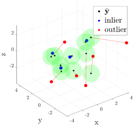
Figure 2: A visualization of the linear regression problem with a 60% outlier rate is shown here. Only 10 measurements are shown for clear representation. The locations of the noise-free measurements, ${\bar{\mbf{y}}}$, are shown as black dots with their 99.73% confidence bounds displayed as green spheres around each measurement. The noisy inlier and outlier measurements are shown in blue and red dots, respectively, and are connected to the associated noise-free measurement via a red line.

IV-A Linear Regression Problem

Consider the following problem

$$\mbf{A}\mbf{x} =\mbf{y},$$ (42)

where ${\mbf{x}}$ is the state to be estimated and ${\mbf{y}}$ are ${n}$-dimensional measurements. The noise free measurements, ${\bar{\mbf{y}}}$, are corrupted by isotropic Gaussian noise, ${\delta\mbf{y}\sim\mathcal{N}(\mbf{0},\bm{\Sigma})}$, such that ${\mbf{y}=\bar{\mbf{y}}+\delta\mbf{y}}$. The corresponding error function for the ${i}$-th measurement is thus

$$\mbf{e}\left(\mbf{y}_{i},\mbf{x}\right)=\mbf{A}_{i}\mbf{x}-\mbf{y}_{i}.$$ (43)

Note that the state ${\mbf{x}}$, the measurement ${\mbf{y}_{i}}$, and the error ${\mbf{e}}$ are all unitless. The residual to this problem is defined according to (1), with the measurement covariance, ${\bm{\Sigma}=\sigma^{2}\mbf{1}}$. Some of these measurements are randomly selected and modified as outliers, ${\mbf{y}^{\textrm{out}}}$, that satisfy

$$\left\|\mbf{e}\left(\mbf{x},\mbf{y}_{i}^{\textrm{out}}\right)\right\|_{{\bm{\Sigma}}^{-1}}^{2}>\chi^{2}\left(n,0.9973\right),$$ (44)

where ${\chi}^{2}(n,0.9973)$ represents the 99.73% probability of the inverse cumulative distribution function of the ${\chi^{2}}$ distribution with ${n}$ degrees of freedom.

IV-A1 Experiment Setting

For this experiment, $1\text{\times}{10}^{3}\text{\,}$ measurements were generated with ${n=3}$ and ${\sigma=0.1}$. A total of 20 Monte Carlo trials were performed for each outlier rate that increased from 20% to 80% in 20% increments. For each outlier rate, the loss functions were tested until convergence without any prior state estimate. For the proposed methods, the shape function from Example III.2 was used. To obtain the initial residual distribution, ${q(\bm{\epsilon})}$, the initial state is obtained using the pseudoinverse of ${\mbf{A}}$. For the loss functions that are based on [6], the truncation bound parameter is set as ${\tau=40}$. Figure 2 shows the setup for a single trial with a 60% outlier rate.

Two convergence criteria are used to determine the termination of the GNC optimization: binary weights and minimum cost difference. The binary weights criterion terminates the optimization when ${w_{i}<\epsilon_{b}}$ or ${w_{i}>1-\epsilon_{b}}$ for all weights. The minimum cost difference criterion terminates the optimization when there exists any cost difference between the current iteration and the last five consecutive iterations that is less than ${\epsilon_{c}}$. For this experiment, ${\epsilon_{b},\epsilon_{c}=$1\text{\times}{10}^{-10}\text{\,}$}$ are used.

IV-A2 Results

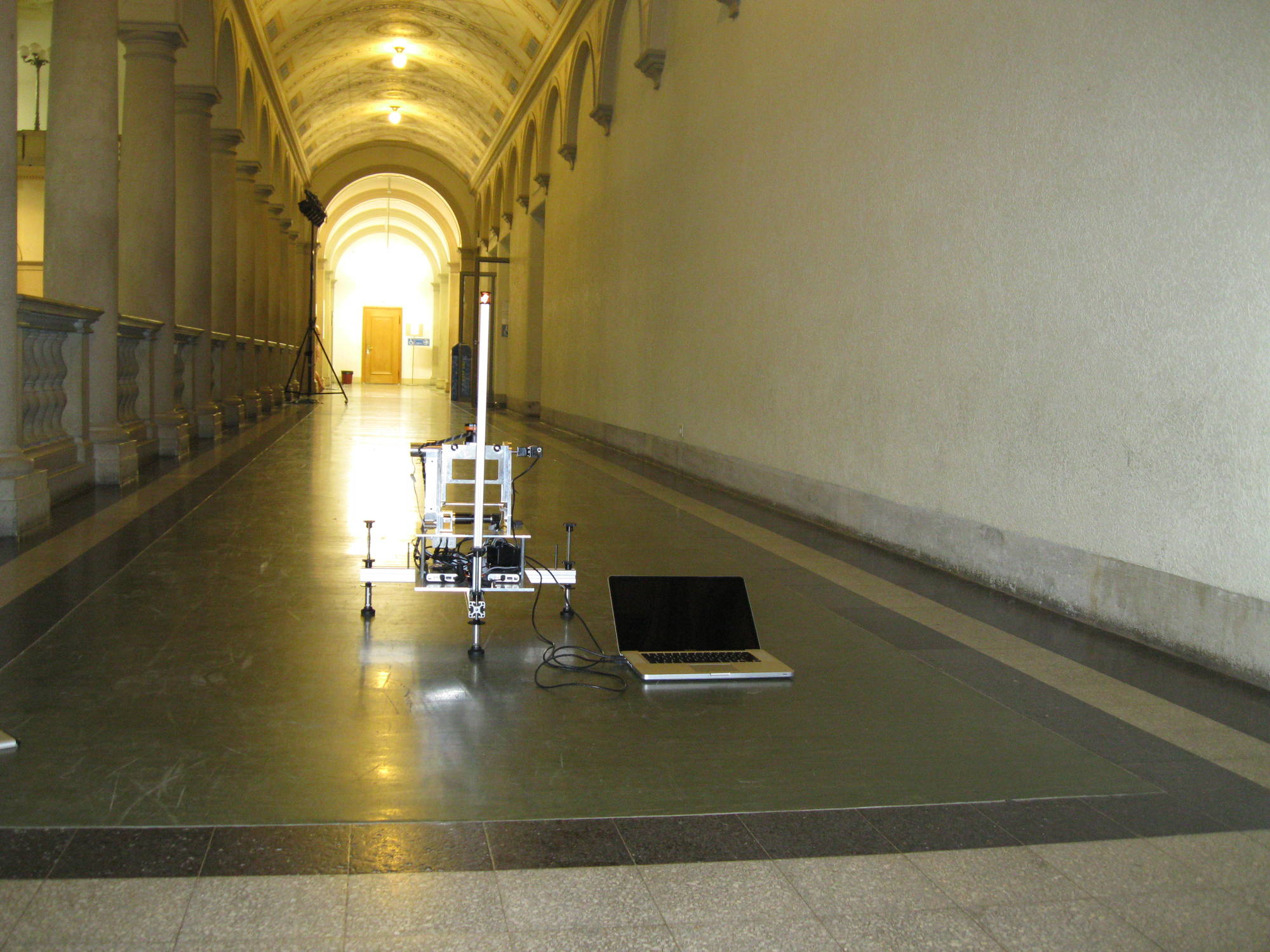
(a) ETH Hauptgebaude (EH)

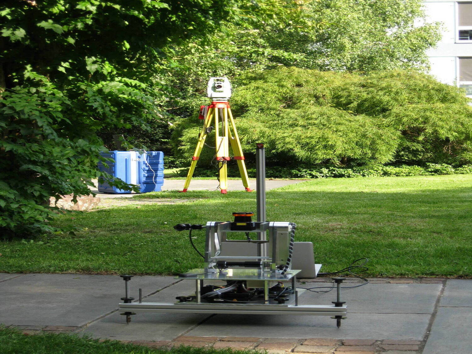
(b) Gazebo in Summer (GZ)

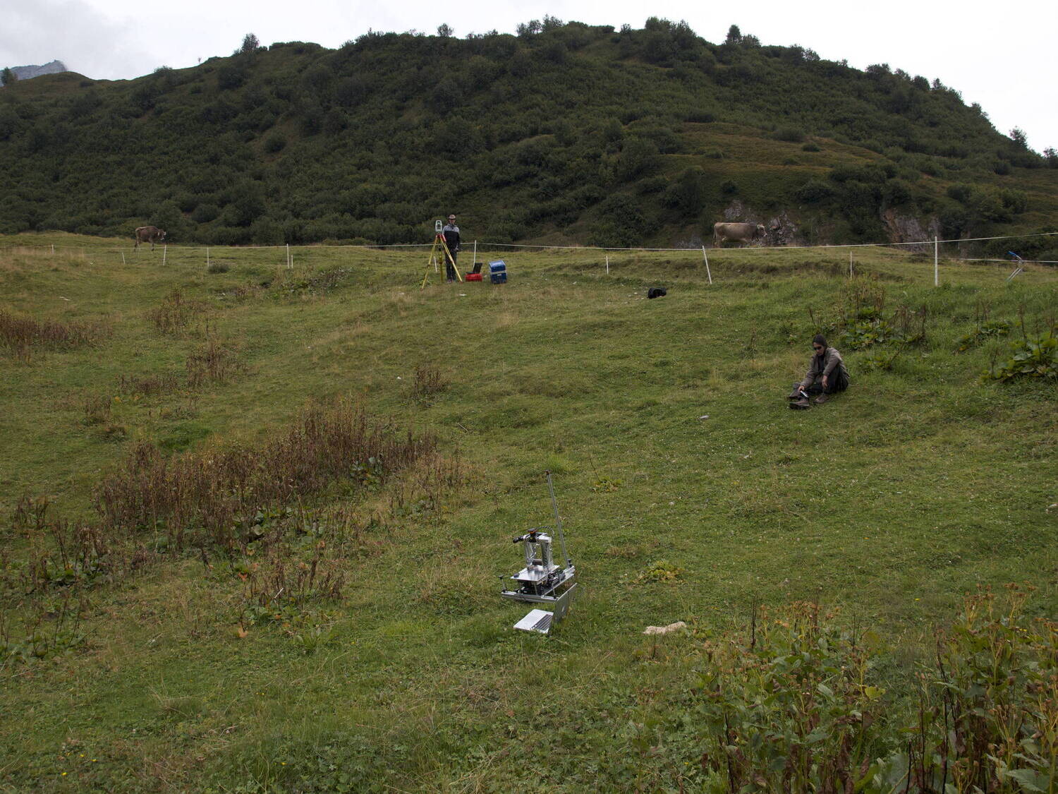
(c) Mountain plain (MP)

Figure 3: Contextual photographs of different environments [14].

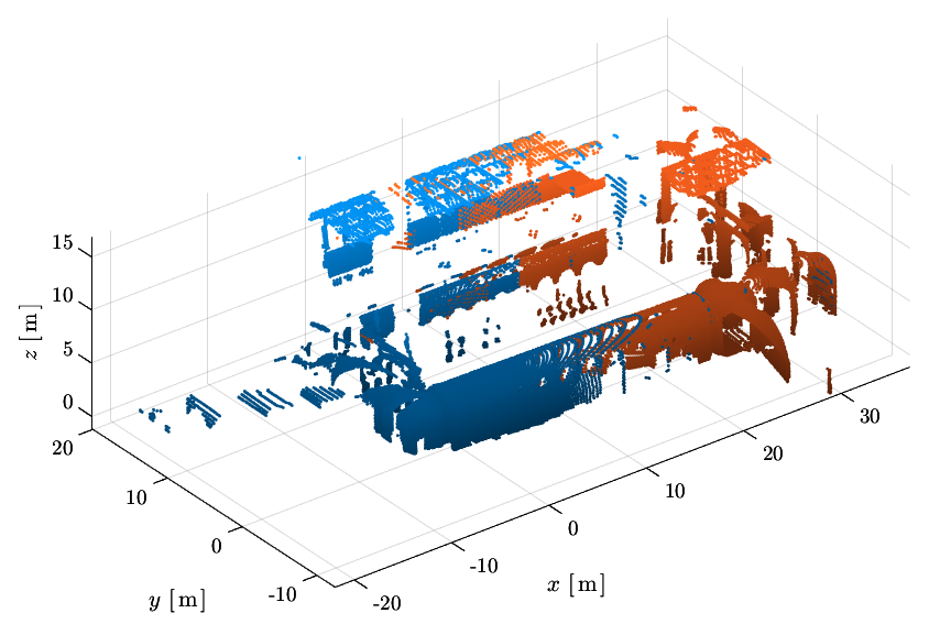
(a) 10%

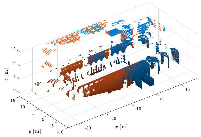
(b) 50%

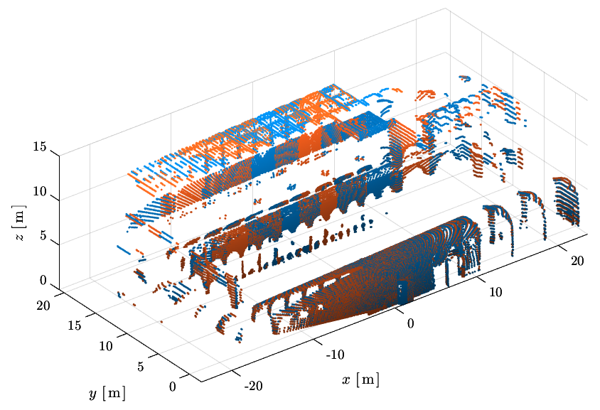
(c) 90%

Figure 4: Three point-cloud scan pairs at different overlap ratio from ETH Hauptgebaude dataset.

Table II shows the linear regression problem results for the traditional loss functions and the corresponding GNC-variants using the method proposed in Section III. GNC variants of Cauchy, Welsch, and GM are AGNC with ${\alpha=0}$, ${\alpha=-\infty}$, and ${\alpha=2}$, respectively [5]. GNC variants of BA/CA and AMB are AGNC with ${\alpha^{\star}}$ and ${a^{\star}}$ obtained using (21) and (19), respectively. Overall, GNC variants outperform other non-GNC-based counterparts at the expense of longer processing time. For example, AMB, the best-performing method amongst the traditional loss functions in terms of the median error, produces higher errors than most of the GNC-incorporated methods. This behaviour is expected when non-GNC loss functions are optimized without an accurate prior estimate because nonminimal solvers are only able to obtain locally optimal solutions.

Note that G-GM method is on par with the G-GM method proposed by [8] in terms of the median error but requires a quarter of the processing time. This is due to the convergence rate of the AGNC loss function, which can be controlled by the amount of nonconvexity added, which is governed by the choice of the shape function ${f(\cdot)}$ as discussed in Section III-A.

The AGNC loss function with various ${\alpha^{\star}}$ values is compared with GNC-TLS and GNC-AMB in Table III. GNC-Cauchy produces the lowest median error in most of the outlier levels with the lowest processing time around $0.13\text{\,}\mathrm{s}$. GNC-TLS requires twice the processing time as AGNC, but outperforms GNC-${\alpha^{\star}}$ at the 80% outlier level.

In [5] and [7], it is pointed out that as the percentage of outliers increases, the shape parameter ${\alpha^{\star}}$ approaches negative infinity, causing the weights assigned to the inlier residuals around the mode ${\tilde{\epsilon}}$ to be indistinguishable from the weights assigned to the outlier residuals. Similar behaviour is observed with GNC-Welsch in Table III. Thus, AGNC with ${\alpha\geq{0}}$ generally performs well with outlier levels of 40% and 60%.

Although GNC-AMB delivers higher median errors on average when compared to other GNC methods, the error variance is generally lower, as well as the median error at higher outlier rates. For GNC-AMB, 90% of the error falls below 7.78 at a 60% outlier level while GNC-TLS falls under 8.37. Also, GNC-AMB has the second-lowest 90% error percentile at an 80% outlier level as shown at the bottom of the right most column in Table III, with almost half the processing time of GNC-TLS.

IV-B Point-Cloud Alignment

Point-cloud alignment (PCA) is an algorithm used to find a 3D rigid transformation that best aligns two input point clouds. The two point clouds are a fixed point cloud, ${\mathcal{P}=\{\mbf{r}^{p_{i}s_{1}}_{\ell_{1}}\}^{N}_{i=1}}$, and a moving point cloud, ${\mathcal{Q}=\{\mbf{r}^{q_{i}s_{2}}_{\ell_{2}}\}^{M}_{i=1}}$. The point measurement ${\mbf{r}^{p_{i}s_{1}}_{\ell_{1}}}$ describes the position of the ${i}$-th point ${p_{i}}$ relative to the position of the sensor ${s_{1}}$ resolved in the sensor frame ${\mathcal{F}_{\ell_{1}}}$ at time ${t_{1}}$. The relative transformation is represented as an element of matrix Lie group ${SE(3)}$,

$$\mbf{T}^{s_{2}s_{1}}_{\ell_{1}\ell_{2}} =\begin{bmatrix}\mbf{C}_{\ell_{1}\ell_{2}}&\mbf{r}^{s_{2}s_{1}}_{\ell_{1}}\\ \mbf{0}&1\end{bmatrix}\in SE(3),$$ (45)

where ${\mbf{C}\in SO(3)=\{\mbf{C}\in\mathbb{R}^{3\times 3}\ |\ \mbf{C}\mbf{C}^{{\mathsf{T}}}=\mbf{1},\det\mbf{C}=+1\}}$ is the direction cosine matrix that represents the attitude of the laser frame at ${t_{2}}$ with respect to the laser frame at ${t_{1}}$, and ${\mbf{r}^{s_{2}s_{1}}_{\ell_{1}}\in\mathbb{R}^{3}}$ represents the position of the sensor at time ${t_{2}}$ relative to the sensor at time ${t_{1}}$, resolved in the sensor frame at time ${t_{1}}$. For readability, ${\mbf{T}_{12}=\mbf{T}^{s_{2}s_{1}}_{\ell_{1}\ell_{2}}}$.

The iterative closest point (ICP) algorithm is used to solve a PCA problem herein. The ICP algorithm solves a nonconvex optimization problem, thus it is often solved iteratively from a prior relative transformation ${\check{\mbf{T}}_{12}}$. The algorithm first associates each point in ${\mathcal{P}}$ to its nearest Euclidean neighbour in ${\mathcal{Q}}$ using ${\mbf{T}_{12}}$. The associated points in ${\mathcal{Q}}$ are now denoted as ${\tilde{\mathcal{Q}}=\{\mbf{r}^{q_{i}s_{2}}_{\ell_{2}}\}^{N}_{i=1}}$ where ${N}$ is the total number of point correspondences. Then, the optimization problem

$$\mbf{T}_{12}^{\star}=\underset{\mbf{T}_{12}\in SE(3)}{\operatorname*{arg\,min}}\sum_{i=1}^{N}\frac{1}{2}w_{i}\left\|\mbf{e}_{i}\left(\mbf{T}_{12},\mbf{r}^{p_{i}s_{1}}_{\ell_{1}},\mbf{r}^{q_{i}s_{2}}_{\ell_{2}}\right)\right\|_{\bm{\Sigma}^{-1}_{i}}^{2}$$ (46)

is solved, where ${w_{i}\in(0,1]}$ are association weights, ${\mbf{e}_{i}}$ are association errors, and ${\bm{\Sigma}_{i}}$ are association error covariances. Then, the point correspondences are found again with the updated relative transformation. When GNC is applied to the ICP algorithm, the minimization problem in (46) is solved using the GNC algorithm.

IV-B1 Experiment Setting

An open-source point-cloud data was used in this experiment [14]. The dataset contains eight point-cloud sequences where each sequence contains ground-truth poses, point-cloud scans, and the overlap ratio between scan pairs. Recall that naively solving (46) can lead to a poor estimate in the presence of outlier correspondences. Outlier correspondences are frequently found in the case of poor ICP initialization, or when there is a low overlap ratio between ${\mathcal{P}}$ and ${\mathcal{Q}}$. Thus, to thoroughly evaluate the proposed loss functions, ICP performance is evaluated subject to three input setting: the environment diversity, the overlap ratio, and the initial perturbation.

Three point-cloud datasets were chosen from [14], representing a wide range in the diversity of the scanned environment. “ETH Hauptgebaude” (EH) was chosen to represent structured scans, while “Gazebo in Summer” (GZ) and “Mountain Plain” (MP) were chosen to represent semi-structured and unstructured scans, respectively. The “structured” level is a qualitative assessment of the number of geometric primitives visible in the scene. The datasets are shown in Figure 3.

TABLE IV: ICP experiment setting.

Downsample	VoxelGrid with $10\text{\,}\mathrm{cm}$ voxel size
Normals	15 nearest neighbours
Point association	Single nearest neighbour
Residual	Point-to-plane error
Convergence	${\left\|\delta\bm{\phi}^{\star}\right\|<$1\text{\times}{10}^{-3}\text{\,}\mathrm{rad}$}$
	${\left\|\delta\bm{\rho}^{\star}\right\|<$1\text{\times}{10}^{-3}\text{\,}\mathrm{m}$}$
Maximum iterations	50

For each point-cloud sequence, two scans are randomly selected to represent ${\mathcal{P}}$ and ${\mathcal{Q}}$, and the selected scan pair is assigned to the corresponding overlap ratio bins. The bins span from 30% to 90% with a bin size of 20%. An example of scan pairs with different overlap ratio is shown in Figure 4.

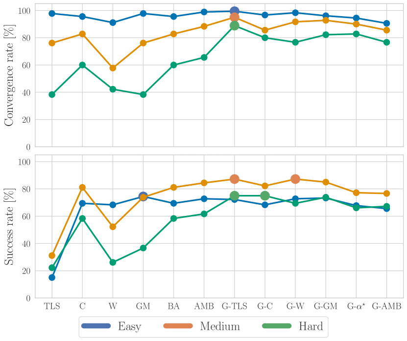
Figure 5: The percentage of ICP convergence and success for every RLF candidate for various initial perturbations in all environments and overlap ratio. ICP is considered successful if both the final rotation and translation errors are less than the initial perturbation, ${\|\delta\hat{\bm{\phi}}\|<\|\delta\check{\bm{\phi}}\|}$ and ${\|\delta\hat{\bm{\rho}}\|<\|\delta\check{\bm{\rho}}\|}$, and the total number of iteration is less than the maximum specified in Table IV. The method with the highest percent convergence and success rate are shown in bold for each difficulty level.

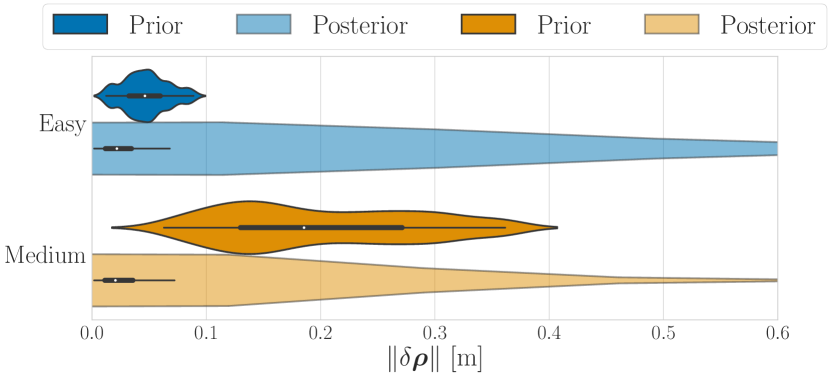
Figure 6: Prior and posterior translation error distribution for easy and medium difficulty levels for all RLFs with EH dataset.

For each scan pair, three levels of initial relative transformation difficulty are tested: “low,” “medium,” and “high.” The initial relative transformation is computed using ${\check{\mbf{T}}_{12}=\mbf{T}_{12}\delta\check{\mbf{T}}}$, where ${\mbf{T}_{12}}$ is the ground-truth transformation and ${\delta\check{\mbf{T}}}$ is the initial perturbation defined in the matrix Lie algebra ${\mathfrak{se}(3)}$ [15],

$$\log\left(\delta\check{\mbf{T}}\right)=\delta\check{\bm{\xi}}^{\wedge}=\begin{bmatrix}\delta\check{\bm{\phi}}\\ \delta\check{\bm{\rho}}\end{bmatrix}^{\wedge}\in\mathfrak{se}(3),$$ (47)

where ${(\cdot)^{\wedge}:\mathbb{R}^{6}\to\mathfrak{se}(3)}$ is an isometric operator, and ${\delta\bm{\phi}}$ and ${\delta\bm{\rho}}$ represent the perturbation in rotation and translation in ${\mathfrak{se}(3)}$, respectively. Thus, the perturbation $\delta\check{\mbf{T}}$ is composed of

$$\delta\check{\bm{\phi}}\sim\mathcal{N}\left(\mbf{0},\sigma_{\phi}^{2}\mbf{1}\right),\quad\delta\check{\bm{\rho}}\sim\mathcal{N}\left(\mbf{0},\sigma_{\rho}^{2}\mbf{1}\right),$$ (48)

where ${\sigma_{\phi}}$ and ${\sigma_{\rho}}$ are the perturbation standard deviations in the attitude and position, respectively. The standard deviations are chosen from ${\|\delta\check{\bm{\phi}}\|<\delta\phi_{\max}}$ and ${\|\delta\check{\bm{\rho}}\|<\delta\rho_{\max}}$ such that ${\delta\phi_{\max}}$ is $10\text{\,}\mathrm{\SIUnitSymbolDegree}$, $20\text{\,}\mathrm{\SIUnitSymbolDegree}$, and $45\text{\,}\mathrm{\SIUnitSymbolDegree}$, and ${\delta\rho_{\max}}$ is $0.1\text{\,}\mathrm{m}$, $0.5\text{\,}\mathrm{m}$, and $1\text{\,}\mathrm{m}$, for easy, medium, and hard levels, respectively.

For each point-cloud sequence, 20 scan pairs are tested for each perturbation level and scan overlap ratio setting. With 3 point-cloud sequences, 3 scan overlap ratio, and 3 initial perturbation levels, a total of 540 trials were conducted over 12 different RLF candidates. ICP experiment setting are given in Table IV. For the proposed methods, the shape function from Example III.3 is used.

Furthermore, the association error is defined as the point-to-plane error [16]. However, the distribution of point-to-point error [17] is used to compute the shape parameters for the adaptive RLFs such that the distance between two associated points is considered when rejecting outlier matches. The point-to-point error and its squared Mahalanobis are defined as

$$\mbf{e}_{i} =\mbf{r}^{p_{i}s_{1}}_{\ell_{1}}-\left(\mbf{C}_{\ell_{1}\ell_{2}}\mbf{r}^{q_{i}s_{2}}_{\ell_{2}}+\mbf{r}^{s_{2}s_{1}}_{\ell_{1}}\right),$$ (49)

$$\epsilon_{i}^{2} =\mbf{e}_{i}^{{\mathsf{T}}}\bm{\Sigma}_{i}^{-1}\mbf{e}_{i},$$ (50)

where ${\bm{\Sigma}_{i}=\mbf{C}_{\ell_{1}\ell_{2}}\mbf{R}_{p_{i}}\mbf{C}_{\ell_{1}\ell_{2}}^{{\mathsf{T}}}+\mbf{R}_{q_{i}}}$ is the covariance matrix of the ${i}$-th point-to-point error, computed using ${\mbf{R}_{p_{i}}}$ and ${\mbf{R}_{q_{i}}}$, the covariance on the measured points ${p_{i}}$ and ${q_{i}}$, respectively. The covariance of ${p_{i}}$ is set to ${\mbf{R}_{p_{i}}=\mbf{R}_{q_{i}}=\sigma^{2}_{\ell}\mbf{1}}$, where ${\sigma_{\ell}=$3\text{\,}\mathrm{cm}$}$ as reported in [14].

TABLE V: Alignment errors and timing results for successful trials incorporating different RLFs, broken down by environment and difficulty level. The errors are reported as 50%-75%-90% percentiles. The lowest error for each percentile for every dataset and difficulty is highlighted in bold.

Metric	Dataset	Difficulty	GNC-TLS	GNC-Cauchy	GNC-Welsch	GNC-GM	GNC-${\alpha^{\star}}$	GNC-AMB
$\left\|\delta\hat{\bm{\phi}}\right\|$ [$\mathrm{deg}$]	EH	Easy	0.18-0.26-0.31	0.17-0.25-0.30	0.16-0.26-0.32	0.18-0.26-0.31	0.17-0.25-0.31	0.18-0.26-0.31
		Medium	0.14-0.22-0.34	0.14-0.21-0.32	0.14-0.22-0.33	0.14-0.21-0.33	0.14-0.21-0.33	0.14-0.22-0.32
		Hard	0.17-0.21-0.29	0.15-0.20-0.27	0.17-0.21-0.30	0.17-0.20-0.27	0.17-0.21-0.32	0.16-0.20-0.29
	GZ	Easy	0.32-0.50-0.75	0.30-0.45-0.61	0.33-0.46-0.63	0.30-0.44-0.59	0.30-0.42-0.59	0.29-0.43-0.58
		Medium	0.38-0.68-6.94	0.35-0.42-0.59	0.35-0.44-0.74	0.31-0.40-0.55	0.31-0.39-0.57	0.33-0.41-0.57
		Hard	0.58-17.5-31.8	0.44-0.65-16.0	0.43-1.72-15.3	0.41-0.67-15.8	0.51-15.9-26.2	0.37-0.57-9.69
	MP	Easy	0.28-0.38-0.54	0.27-0.44-0.77	0.27-0.42-0.55	0.25-0.37-0.60	0.24-0.38-0.54	0.25-0.40-0.54
		Medium	0.29-0.42-3.71	0.24-0.35-0.47	0.28-0.43-0.57	0.24-0.34-0.43	0.24-0.35-0.47	0.25-0.36-0.47
		Hard	0.39-3.72-13.6	0.33-0.41-1.78	0.35-0.42-0.47	0.39-6.08-14.1	0.32-0.41-2.23	0.31-0.40-0.59
$\left\|\delta\hat{\bm{\rho}}\right\|$ [$\mathrm{cm}$]	EH	Easy	1.98-3.33-5.11	1.83-3.17-4.16	2.22-3.39-5.29	2.10-3.34-5.05	1.88-3.25-4.76	1.95-3.36-5.31
		Medium	2.02-3.42-4.44	1.92-3.00-4.17	2.14-3.72-4.43	2.07-3.41-4.39	1.97-3.32-4.32	1.95-3.32-4.37
		Hard	2.15-4.04-4.92	1.97-3.58-4.77	2.04-3.61-5.01	2.18-4.09-4.95	2.00-4.04-5.13	2.12-3.91-5.25
	GZ	Easy	1.59-2.67-4.33	1.48-2.27-3.18	1.44-2.33-3.66	1.28-1.91-2.80	1.29-1.96-2.62	1.39-1.90-3.00
		Medium	1.75-3.62-45.6	1.28-1.89-3.61	1.58-2.41-3.59	1.19-1.93-3.41	1.39-2.28-3.51	1.24-2.38-3.65
		Hard	3.08-46.3-70.0	1.61-3.29-94.5	1.92-5.64-42.0	1.45-3.07-44.6	2.41-27.9-69.2	1.40-2.54-30.5
	MP	Easy	3.55-5.42-7.28	2.86-4.75-7.57	3.45-5.34-6.98	2.85-4.58-7.50	2.68-4.17-6.48	2.84-3.69-7.28
		Medium	3.93-6.53-12.5	2.41-3.86-6.13	3.01-5.48-8.07	2.52-3.86-5.88	2.38-3.95-5.46	2.38-3.87-6.27
		Hard	4.42-13.4-59.2	3.63-4.42-8.83	3.35-5.11-8.22	4.51-16.8-49.0	3.55-4.49-10.2	3.67-4.23-5.84
Iterations	ALL	ALL	8	6	7	5	5	6
Time [$\mathrm{s}$]	ALL	ALL	17.98	12.24	16.30	17.29	21.17	13.90

IV-B2 ICP Success Rate

ICP is considered to have converged when the incremental update ${\delta\bm{\xi}^{\star}}$ is less than the convergence thresholds defined in Table IV before the maximum number of iterations. However, each trial is considered “successful” when both posterior errors, ${\delta\hat{\bm{\phi}}}$ and ${\delta\hat{\bm{\rho}}}$, are less than the initial perturbations, and the total number of iterations is less than the maximum threshold specified in Table IV. The top plot of Figure 5 shows the convergence rate of each method at different difficulty levels, whereas the bottom figure shows the success rate. The method with the highest percent convergence and success rate are shown in bold for each difficulty level in Figure 5. Note that the success rate for the “easy” initial perturbations performs worse than medium difficulty. This happens more often with the “easy” difficulty level since the initial perturbation is small, but the posterior error is not significantly different from the prior as shown in Figure 6.

GNC-TLS outperforms other methods in terms of both convergence and success rate for medium and hard difficulty levels followed by GNC-Welsch. GNC-incorporated methods generally outperform the baseline robust loss functions especially in the hard difficulty level showing that the GNC-incorporated methods are more robust to both initial perturbation and environment diversity. Thus, for further analysis of the results, GNC-incorporated methods are discussed more in detail.

IV-B3 Processing Time

Figure 9 shows the number of iterations and convergence time of the successful ICP trials in a log scale. Note that this study was conducted using non-optimized MATLAB code, and timing results are included for relative comparison. Overall, GNC-incorporated methods take fewer iterations but more time to converge than non-GNC methods. Because each ICP least-squares optimization problem is solved gradually from a convex surrogate, each iteration for the GNC-incorporated method takes more time than an iteration of the non-GNC methods.

The nonadaptive RLFs, TLS, Cauchy, and GM, tend to have low convergence time, but also low success rates especially, in higher initial perturbations. GNC-incorporated methods require a significantly longer time to converge, which hinders its practicality in real-time applications. The proposed adaptive GNC methods rival the processing time of GNC-TLS with more robustness to outliers and a large reduction in error variance.

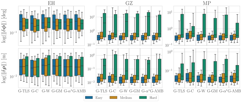
Figure 7: Box plots show ICP alignment errors for different dataset and initial perturbation combinations. Only GNC-incorporated methods are shown as they outperform other non-GNC methods in terms of ICP success rate as shown in Figure 5. Boxes represent the middle 50% of the data, with its median shown as a black line. The whiskers represent 10% and 90% percentiles, and black dots represent the outliers.

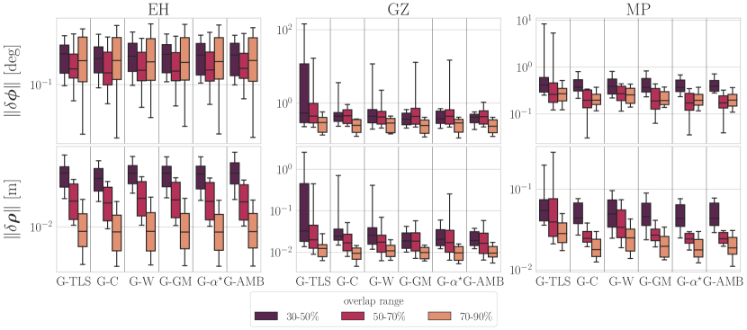
Figure 8: Box plots show ICP alignment errors for different dataset and percent overlap combinations. Boxes represent the middle 50% of the data, with its median shown as a black line. The whiskers represent 10% and 90% percentiles, and black dots represent the outliers.

IV-B4 ICP Alignment Errors

Table V shows the succeeded ICP alignment errors and timing results for each dataset and difficulty combinations. Overall, all GNC loss functions perform well in the structured environments regardless of the initial perturbation, with GNC-Cauchy performing marginally better than the others. However, the difference in performance become more pronounced in semistructured and unstructured environments. Semistructured environment exhibit higher median errors in rotation than the structured environments, whereas unstructured environments exhibit higher median errors in both rotation and translation.

GNC-${\alpha^{\star}}$ and GNC-AMB outperform other methods in semistructured and unstructured environments. In addition, they show lower variance in errors, shown by the 75th and 90th percentiles in Table V. For example, in the experiment with the semistructured “GZ” dataset with the “hard” difficulty level (GZ-Hard), 90% of the rotation error falls below $9.69\text{\,}\mathrm{\SIUnitSymbolDegree}$ with GNC-AMB followed by GNC-Welsch, while GNC-TLS performs with $31.8\text{\,}\mathrm{\SIUnitSymbolDegree}$. Also, 90th percentile of the translation error is $30.5\text{\,}\mathrm{cm}$ with GNC-AMB whereas it is $70.0\text{\,}\mathrm{cm}$ for GNC-TLS.

The experiment with the unstructured “MP” dataset and “hard” difficulty level also shows the similar trend. The 90th percentile rotation error for GNC-AMB, $0.59\text{\,}\mathrm{\SIUnitSymbolDegree}$, is significantly lower than $13.6\text{\,}\mathrm{\SIUnitSymbolDegree}$ of GNC-TLS. The GNC-AMB loss function realizes a notable variance reduction with translation error of $5.84\text{\,}\mathrm{cm}$ at 90th percentile in comparison to $59.2\text{\,}\mathrm{cm}$ of GNC-TLS.

The variance reduction in the proposed methods is shown in more detail in Figure 7, where the whiskers represent 10th and 90th percentiles. GNC-GM and GNC-AMB performs with the lowest 90th percentile error in both rotation and translation for medium and hard difficulty levels, respectively. Furthermore, GNC-Cauchy performs with the lowest processing time of $12.24\text{\,}\mathrm{s}$ followed by GNC-AMB with $13.90\text{\,}\mathrm{s}$ per optimization.

The proposed GNC-${\alpha^{\star}}$ outperforms the state-of-the-art GNC-TLS in both median and variance of the errors in all experiments. However, GNC-AMB realizes faster, more robustness, and accuracy estimates than GNC-${\alpha^{\star}}$ by applying a norm-aware loss function.

IV-B5 Overlap Ratio

Outlier measurements are often found when the amount of overlap between a scan pair is low. Figure 8 shows that the performance of all RLFs generally improves with with increasing percent overlap. The reduction in translation error with increasing overlap is especially notable in the structured “EH” environment, in which geometric primitives such as planes may lead to strong local minima. Again, GNC-AMB outperforms all other methods in semistructured and unstructured environments in terms of both median and variance of the errors. The difference is more pronounced in 30%-50% overlap ratio.

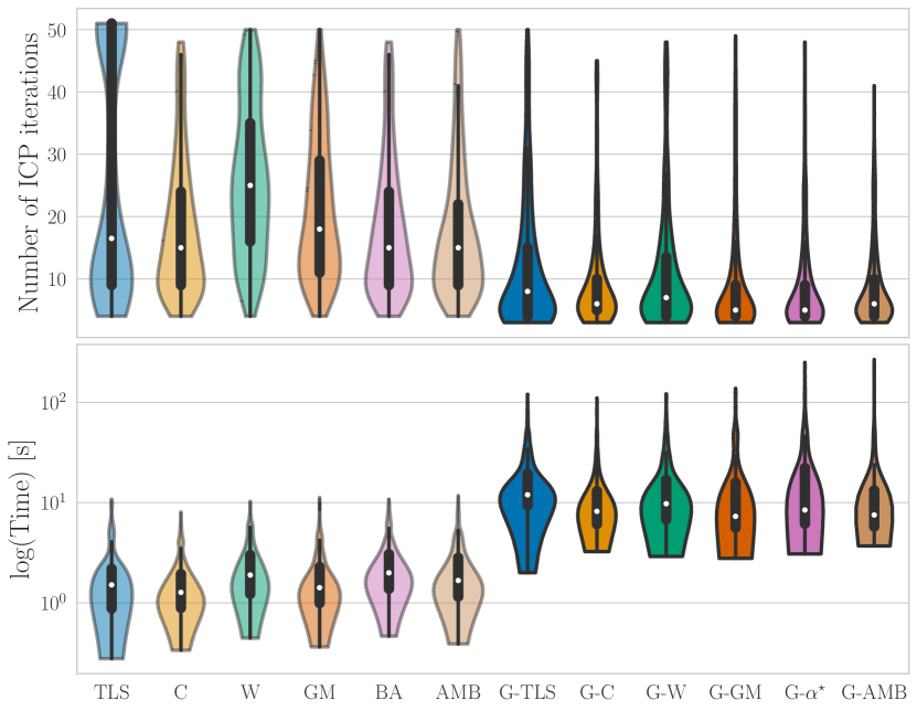
Figure 9: Violin plots show the number of iterations and convergence time of the successful ICP trials. The times are shown in a log scale for clear representation. The corresponding baseline functions are shown in the same color with lower opacity. The width of each violin distribution is proportional to the number of successful trials.

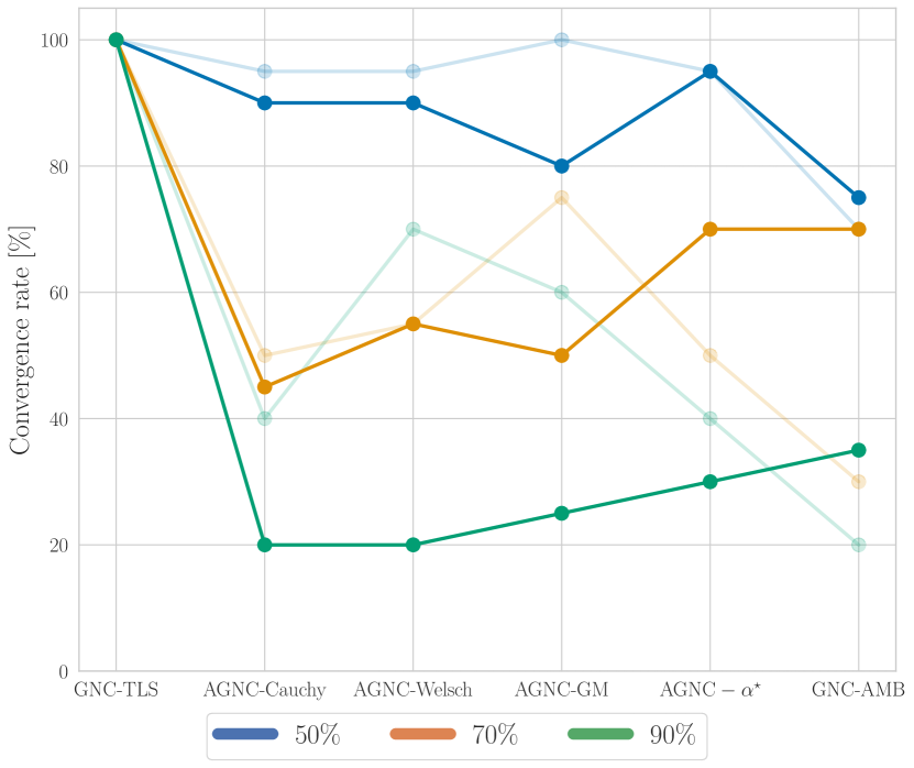
Figure 10: Mesh registration convergence for every baseline robust loss functions (transparent) and their GNC variants (opaque) are shown for different outlier ratio. The SDP solver is considered converged when the relative change in the objective function is less than $1\text{\times}{10}^{-8}\text{\,}$.

IV-C Mesh Registration

Mesh registration is an algorithm used to find a 3D rigid transformation ${\mbf{T}^{c_{m}c_{p}}_{mp}\in SE(3)}$ between a 3D mesh and a point cloud, where ${c_{m}}$ and ${c_{p}}$ are the centroids of mesh and point cloud, respectively. A mesh ${\{\{\mbf{r}^{q_{ij}c_{m}}_{m}\}_{j=1}^{M_{i}},\mbf{n}^{m_{i}}_{m}\}_{i=1}^{N_{s}}}$ is represented as a collection of ${N}_{s}$ surfaces with corresponding unit normal vector ${\mbf{n}^{m_{i}}_{m}}$ resolved in the mesh frame ${\mathcal{F}_{m}}$. Each surface is represented as a set of vertices ${\{\mbf{r}^{q_{ij}c_{m}}_{m}\}_{j=1}^{M_{i}}}$ where ${M_{i}}$ is the number of vertices for ${i}$-th surface, and ${q_{ij}}$ is the ${j}$-th vertex of ${i}$-th surface. A point cloud is ${\{\mbf{r}^{p_{i}c_{p}}_{p},\mbf{n}^{p_{i}}_{p}\}_{i=1}^{N_{p}}}$ is represented as a collection of ${N_{p}}$ points with estimated normals ${\mbf{n}^{p_{i}}_{p}}$ resolved in the point cloud frame ${\mathcal{F}_{p}}$. For the brevity of notation, ${\mbf{T}_{mp}=\mbf{T}^{c_{m}c_{p}}_{mp}}$, ${\mbf{r}^{pm}_{m}=\mbf{r}^{c_{p}c_{m}}_{m}}$, ${\mbf{r}^{i}_{p}=\mbf{r}^{p_{i}c_{p}}_{p}}$, ${\mbf{n}^{i}_{m}=\mbf{n}^{m_{i}}_{m}}$, and ${\mbf{n}^{i}_{p}=\mbf{n}^{p_{i}}_{p}}$.

The least squares formulation for the mesh registration problem is based on [8]. Given a set of ${N}$ putative correspondences from a point cloud to a mesh, mesh registration finds the rigid body transformation that best aligns the point cloud to the mesh by solving

$$\mbf{T}^{\star}_{mp} =\underset{\mbf{T}_{mp}\in SE(3)}{\operatorname*{arg\,min}}\sum_{i=1}^{N}\mbox{$\textstyle{\frac{1}{2}}$}w_{i}\left(\frac{1}{\sigma^{pi}_{p}}{e^{i}_{p}}^{2}+\left\|\mbf{e}^{i}_{n}\right\|_{{\bm{\Sigma}^{i}_{n}}^{-1}}\right),$$ (51)

where ${\sigma_{p}^{pi}}$ and ${\bm{\Sigma}^{i}_{n}}$ are the covariance associated with the point-to-plane and normal-to-normal distance, given respectively as

$$e^{i}_{p}\left(\mbf{T}_{mp},\tilde{\mbf{r}}^{i}_{m},\mbf{r}^{i}_{p},\mbf{n}^{i}_{m}\right) ={\mbf{n}^{i}_{m}}^{{\mathsf{T}}}\left(\mbf{C}_{mp}\mbf{r}^{i}_{p}+\mbf{r}^{pm}_{m}-\tilde{\mbf{r}}^{i}_{m}\right),$$ (52)

$$\mbf{e}^{i}_{n}\left(\mbf{T}_{mp},\mbf{n}^{i}_{m},\mbf{n}^{i}_{p}\right) =\mbf{n}^{i}_{m}-\mbf{C}_{mp}\mbf{n}^{i}_{p}.$$ (53)

For each point-to-face association, an arbitrary point ${\tilde{\mbf{r}}^{i}_{m}}$ is chosen from the corresponding surface.

Unlike PCA, the mesh registration experiment is performed on sparse point-to-face correspondences to test the robustness of the loss functions. For the proposed methods, shape functions from Example III.1 and III.2 were used and tested in simulation and in an experimental setting, respectively.

IV-C1 Simulation Setting

The simulation setup is based on [18]. A set of ${N=20}$ 3D planes ${\{\mbf{r}^{i}_{m},\mbf{n}^{i}_{m}\}_{i=1}^{N}}$ are randomly generated, where the points are sampled from ${\mbf{r}^{i}_{m}\sim\mathcal{N}(\mbf{0},\mbf{1})}$. Then, a random point on a surface for each ${\mbf{r}^{i}_{m}}$ is generated via ${\tilde{\mbf{r}}^{i}_{m}=\mbf{r}^{i}_{m}+{\mbf{w}^{i}_{m}}^{\times}\mbf{n}^{i}_{m}}$, where ${\mbf{w}^{i}_{m}\sim\mathcal{N}(\mbf{0},\mbf{1})}$. Using an arbitrary rigid body transformation ${\mbf{T}_{mp}}$, a corresponding point cloud ${\{\mbf{r}^{i}_{p},\mbf{n}^{i}_{p}\}}$ is generated by

$$\begin{bmatrix}{\mbf{r}^{i}_{p}}\\ 1\end{bmatrix} =\mbf{T}_{mp}^{-1}\begin{bmatrix}{\mbf{r}^{i}_{m}}\\ 1\end{bmatrix}+\begin{bmatrix}{\bm{\sigma}^{pi}_{p}}\\ 0\end{bmatrix},$$ (54)

$$\mbf{n}^{i}_{p} =\frac{\mbf{C}_{mp}^{{\mathsf{T}}}\mbf{n}^{i}_{m}+\bm{\sigma}^{ni}_{p}}{\left\|\mbf{C}_{mp}^{{\mathsf{T}}}\mbf{n}^{i}_{m}+\bm{\sigma}^{ni}_{p}\right\|},$$ (55)

where ${\bm{\sigma}^{pi}_{p},\bm{\sigma}^{ni}_{p}\sim\mathcal{N}(\mbf{0},0.01^{2}\mbf{1})}$. Note that both generated mesh and point cloud are unitless. Given the mesh and the noisy point cloud, (51) is solved using the mosek SDP solver, as was done in [18]. No initial transformation between the point cloud and the mesh is provided to the solver.

The performance of the solver is evaluated using the estimation error, ${\log(\delta\mbf{T})=\log({\mbf{T}_{mp}^{-1}\mbf{T}^{\star}_{mp}})\in\mathfrak{se}(3)}$, where ${\mbf{T}_{mp}}$ is the ground-truth transformation, and the processing time. For simulation experiments, statistics are computed over 20 Monte Carlo runs per setup as done in [8]. Each setup was performed over various outlier ratio that increases from 50% to 90% in 20% increments.

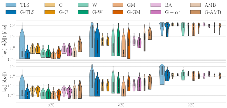
Figure 11: Violin plots show mesh registration errors of each robust loss functions in different outlier levels. The corresponding baseline functions are shown in the same color with lower opacity.

TABLE VI: Simulated mesh registration results of the proposed GNC-AMB and AGNC loss functions with various ${\alpha^{\star}}$. Error percentiles, mean processing times, and median numbers of iterations to converge are shown in different outlier ratio and compared with those of GNC-TLS. The lowest error in each percentile as well as the lowest time and iteration are highlighted in bold.

Metric	Outlier	GNC-TLS	GNC-Cauchy	GNC-Welsch	GNC-GM	GNC-${\alpha^{\star}}$	GNC-AMB
$\left\|\delta\hat{\bm{\phi}}\right\|$ [$\mathrm{deg}$]	50%	0.292-0.353-1.308	0.775-1.273-2.038	0.300-0.467-1.352	0.415-0.597-1.032	0.695-1.314-1.959	1.634-4.110-8.034
	70%	1.272-5.082-139.3	3.667-5.799-9.496	2.246-8.558-138.5	3.273-6.543-23.93	3.508-5.653-8.137	18.97-21.78-37.19
	90%	102.9-129.2-166.3	113.8-145.7-161.5	121.9-161.1-163.6	104.3-131.6-153.2	105.9-127.0-132.4	105.1-111.9-134.2
$\left\|\delta\hat{\bm{\rho}}\right\|$	50%	0.010-0.020-0.067	0.044-0.061-0.077	0.013-0.022-0.031	0.022-0.027-0.035	0.032-0.053-0.069	0.059-0.178-0.265
	70%	0.034-0.414-1.938	0.132-0.200-0.439	0.070-0.396-1.863	0.132-0.395-0.897	0.160-0.444-0.663	0.554-0.845-1.102
	90%	1.798-3.217-4.037	1.337-1.666-1.881	1.754-2.393-2.850	1.380-1.566-2.809	2.096-2.834-3.282	1.255-1.731-2.151
Iterations	ALL	10	24	32	34	35	35
Time [$\mathrm{s}$]	ALL	23.04	53.53	63.72	71.24	70.48	72.38

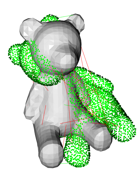
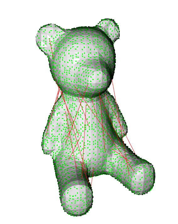
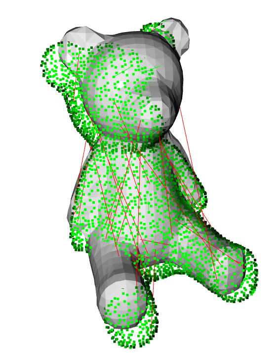
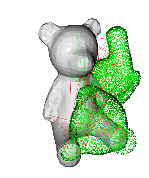
(a) Prior

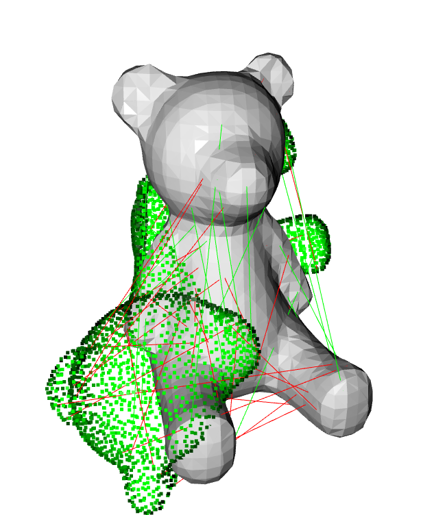
(b) GNC-TLS

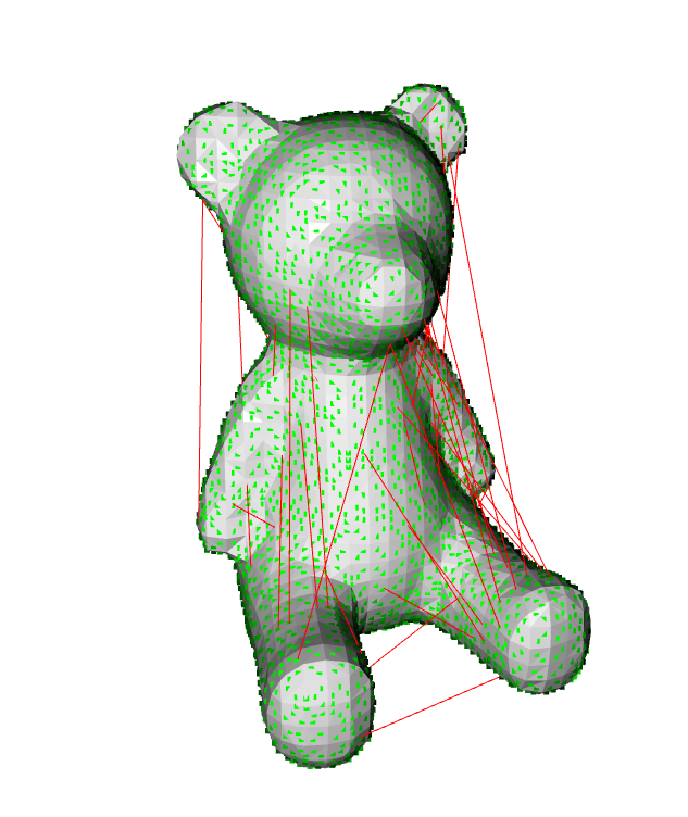
(c) AGNC-${\alpha^{\star}}$

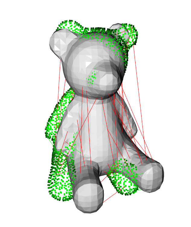
(d) GNC-AMB

Figure 13: Mesh registration results of GNC-TLS, GNC-${\alpha^{\star}}$, and GNC-AMB with ${N=100}$ point-to-face correspondences. The results are shown for 50% (top) and 70% (bottom) outlier ratio.

TABLE VII: Mesh registration results using HomebrewedDB dataset. The mean of the converged rotation and translation errors at 50% and 70% outlier levels are compared.

Metric	Outlier	GNC-TLS	GNC-${\alpha^{\star}}$	GNC-AMB
$\|{\delta\hat{\bm{\phi}}}\|$ [$\mathrm{deg}$]	50%	0.962	0.009	16.87
	70%	24.56	0.002	28.57
$\|{\delta\hat{\bm{\rho}}}\|$	50 %	0.202	0.004	13.52
	70%	7.87	0.001	12.85
Time [$\mathrm{s}$]	ALL	103.31	47.10	113.31
Convergence [%]	ALL	100	25	45

IV-C2 Simulation Results

The SDP solver is considered to have converged when the difference in cost between two consecutive iterations is less than $1\text{\times}{10}^{-8}\text{\,}$ before the maximum number of iterations is reached. The convergence rate of the loss functions for different outlier ratio is shown in Figure 10. The TLS and GNC-TLS loss functions exceed all other methods by always converging to a solution regardless of the outlier ratio. GNC variants of Cauchy, Welsch, and Geman-McClure loss functions generally perform poorly in terms of convergence rate compared to its baseline counterparts. On the other hand, the adaptive loss functions like GNC-${\alpha^{\star}}$ and GNC-AMB show increased convergence rate in all outlier levels.

Figure 11 shows the registration errors of each loss function over different outlier ratio. The GNC variants outperform most of their baseline counterparts in both median error and error variance. Table VI shows the median rotation and translation errors and processing time of the GNC-incorporated loss functions. All methods perform poorly in rotation estimation in the presence of high outlier ratio. However, GNC-TLS yields the lowest median error and processing time followed by GNC-Welsch in almost all experiments. The GNC variants of Cauchy, Welsch, and Geman-McClure loss functions perform better than their the adaptive loss functions GNC-${\alpha^{\star}}$ and GNC-AMB. The estimation accuracy of GNC-${\alpha^{\star}}$ and GNC-AMB decreases when the number of correspondences are too low to formulate a meaningful statistics of the residuals.

However, the error variance in GNC-TLS is very high compared to the proposed methods. At 90% outlier ratio, 90% of the translation error fall within $1.881\text{\,}\mathrm{m}$ for GNC-Cauchy while 90% of the error fall within $4.037\text{\,}\mathrm{m}$ for GNC-TLS. The rotation errors follow a similar pattern. The 90th percentile of GNC-${\alpha^{\star}}$ rotation errors fall below $8.137\text{\,}\mathrm{\SIUnitSymbolDegree}$ for 70% outlier ratio experiment while GNC-TLS yields $139.3\text{\,}\mathrm{\SIUnitSymbolDegree}$. Despite having low convergence rate and low median error, the proposed methods outperform GNC-TLS in error variance.

The success rate with GNC-TLS is very high compared to the proposed methods. This means that GNC-TLS is able to converge to a solution regardless of the global optimality. Although the convergence rates of GNC-${\alpha^{\star}}$ methods are low, the low error variance shows that the method is able to converge with high precision.

IV-C3 Experiment Setting

The HomebrewedDB dataset [19] is used to evaluate the performance of the proposed robust loss functions on real-world data. Among the 33 objects featured by the dataset, “Teddy Bear” mesh is used.

First, a noisy point cloud is generated by sampling points from the centre of each surface of the mesh and adding Gaussian noise with standard deviation ${\sigma=0.01}$. The sampled points that are in the mesh frame are transformed to the point cloud frame with randomly chosen ground-truth rigid-body transformation ${\mbf{T}_{mp}\in SE(3)}$ Using the transformed point cloud, surface normals are estimated using the Open3D library [20]. Then, ${N=100}$ point-to-face correspondences are randomly selected with 50% and 70% of them as outliers.

IV-C4 Experiment Results

Table VII shows the mean of the converged rotation and translation errors at 50% and 70% outlier levels for GNC-TLS, GNC-${\alpha^{\star}}$, and GNC-AMB. Similar to the simulation experiment, the convergence rate of the GNC-TLS loss function is significantly higher than the proposed methods. However, the GNC-${\alpha^{\star}}$ loss function yields lower mean rotation and translation errors than GNC-TLS when converged, showing that GNC-${\alpha^{\star}}$ converges to a more accurate solution, if converged. Figure 13 shows the visual comparison of the mesh registration results at 50% (top) and 70% (bottom) outlier levels. Figure 13(b) shows the result of GNC-TLS converging to a suboptimal solution while GNC-${\alpha^{\star}}$ finds the globally optimal solution.

V Conclusion

The adaptive RLF presented in [5] has received ample attention for its adaptability to a wider family of problems and its ability to deal with a larger set of outlier distributions. In this paper, the adaptive RLFs are combined with GNC to solve least-squares problems, realizing enhanced robustness and convergence properties. Moreover, the Gaussian-like assumption on the residual distribution, which most of the existing loss functions are based on, is replaced by a Chi distribution as proposed by [7] to better represent the underlying residual distribution in multivariate problems. By combining GNC and adaptive loss function, the proposed GNC-${\alpha^{\star}}$ loss function is able to solve nonconvex least-squares problems with a large number of outliers more effectively at faster rates than other GNC-based counterparts [8], as well as existing adaptive RLFs [5, 6, 7]. Also, the proposed adaptive GNC loss function is able to optimal solutions with high precision. The results from linear regression, PCA, mesh registration problems suggest that this approach is widely applicable to any least-squares problems in state estimation and robotics.

DeMenezes2021 Neira2001 Roysdon2017

Appendix A Outlier Process Function

The analytical outlier process function ${\Phi_{\rho}(\cdot)}$ is derived based on the algorithm discussed in [9]. Differentiating the cost function in (6) with respect to ${w}$ and ${\epsilon}$ respectively yields

$$\frac{\partial\rho\left(\epsilon\right)}{\partial w} =\mbox{$\textstyle{\frac{1}{2}}$}\epsilon^{2}+\Phi^{\prime}_{\rho}\left(w\right),$$ (56)

$$\frac{\partial\rho\left(\epsilon\right)}{\partial\epsilon} =w\epsilon.$$ (57)

The expected value of the differentiated cost function is ${0}$. Thus, substituting (57) into (56) and rearranging the terms yields

$$\Phi^{\prime}_{\rho}\left(\frac{1}{\epsilon}\frac{\partial\rho\left(\epsilon\right)}{\partial\epsilon}\right) =-\mbox{$\textstyle{\frac{1}{2}}$}\epsilon^{2}.$$ (58)

To find ${\Phi_{\rho}}$, integrate (58) with respect to ${\epsilon}$. To do so, first define a function ${\phi}$ as

$$\phi\left(\epsilon^{2}\right) =\rho\left(\epsilon\right).$$ (59)

Differentiating (59) with respect to ${\epsilon}$ yields

$$2\epsilon\phi^{\prime}\left(\epsilon^{2}\right) =\frac{\partial\rho\left(\epsilon\right)}{\partial\epsilon}.$$ (60)

Thus, (58) can be rewritten as

$$\Phi^{\prime}_{\rho}\left(2\phi^{\prime}\left(\epsilon^{2}\right)\right) =-\mbox{$\textstyle{\frac{1}{2}}$}\epsilon^{2}.$$ (61)

Assuming that ${\phi^{\prime\prime}(\epsilon^{2})\neq 0}$, multiplying ${\phi^{\prime\prime}(\epsilon^{2})}$ on both sides of (61) and integrating with respect to ${\epsilon^{2}}$ yields

$$\int_{-\infty}^{\infty}\Phi^{\prime}_{\rho}\left(2\phi^{\prime}\left(\epsilon^{2}\right)\right)\phi^{\prime\prime}\left(\epsilon^{2}\right)\mathrm{d}\epsilon^{2}=\mbox{$\textstyle{\frac{1}{2}}$}\Phi_{\rho}\left(2\phi^{\prime}\left(\epsilon^{2}\right)\right),$$ (62)

$$\int_{-\infty}^{\infty}-\mbox{$\textstyle{\frac{1}{2}}$}\epsilon^{2}\phi^{\prime\prime}\left(\epsilon^{2}\right)\mathrm{d}\epsilon^{2}=-\mbox{$\textstyle{\frac{1}{2}}$}\epsilon^{2}\phi^{\prime}\left(\epsilon^{2}\right)+\mbox{$\textstyle{\frac{1}{2}}$}\phi\left(\epsilon^{2}\right).$$ (63)

Equating (62) and (63) results

$$\Phi_{\rho}\left(2\phi^{\prime}\left(\epsilon^{2}\right)\right) =-\epsilon^{2}\phi^{\prime}\left(\epsilon^{2}\right)+\phi\left(\epsilon^{2}\right).$$ (64)

The outlier process function is yet expressed as a function of ${w}$. Note that equating (57) and (60) gives

$$2\phi^{\prime}\left(\epsilon^{2}\right) =w,$$ (65)

$$\epsilon^{2} =\phi^{\prime-1}\left(\mbox{$\textstyle{\frac{1}{2}}$}w\right).$$ (66)

Then, the outlier process function ${\Phi_{\rho}(w)}$ can be recovered by substituting (65) and (66) into (64),

$$\Phi_{\rho}\left(w\right) =\phi\left(\phi^{\prime-1}\left(\mbox{$\textstyle{\frac{1}{2}}$}w\right)\right)-\mbox{$\textstyle{\frac{1}{2}}$}w\phi^{\prime-1}\left(\mbox{$\textstyle{\frac{1}{2}}$}w\right).$$ (67)

Notice that ${w}$ is defined in terms of ${\phi^{\prime}(\cdot)}$ in (65). As ${w}$ varies between ${0}$ and ${1}$,

$$\lim_{\epsilon\to{0}}\phi^{\prime}\left(\epsilon^{2}\right) =\mbox{$\textstyle{\frac{1}{2}}$},$$ (68)

$$\lim_{\epsilon\to\infty}\phi^{\prime}\left(\epsilon^{2}\right) =0,$$ (69)

must be satisfied. Also, to ensure that a minimum of (6) exists, ${\Phi^{\prime\prime}\left(w\right)>0}$. Differentiating (61) with respect to ${\epsilon}$ yields

$$4\Phi^{\prime\prime}_{\rho}\left(2\phi^{\prime}\left(\epsilon^{2}\right)\right)\phi^{\prime\prime}\left(\epsilon^{2}\right)\epsilon =-\epsilon,$$ (70)

$$\Phi^{\prime\prime}_{\rho}\left(2\phi^{\prime}\left(\epsilon^{2}\right)\right) =-\frac{1}{4\phi^{\prime\prime}\left(\epsilon^{2}\right)}>0.$$ (71)

Thus, ${\phi^{\prime\prime}(\cdot)}$ must be strictly negative, which satisfies the assumption necessary to derive (62) and (63).

Appendix B AMB Loss Function

The optimal weights derived from the AMB method described in (23) can be rewritten as

$$\tilde{w} =\begin{cases}1&\textrm{if }\epsilon\leq\tilde{\epsilon}\textrm{ or }\alpha^{\star}=2,\\ \frac{2}{(\epsilon-\tilde{\epsilon})^{2}+1}&\textrm{if }\epsilon>\tilde{\epsilon}\textrm{ and }\alpha^{\star}=0,\\ \exp\left(-\mbox{$\textstyle{\frac{1}{2}}$}(\epsilon-\tilde{\epsilon})^{2}\right)&\textrm{if }\epsilon>\tilde{\epsilon}\textrm{ and }\alpha^{\star}=-\infty,\\ \left(\frac{(\epsilon-\tilde{\epsilon})^{2}}{\left|\alpha^{\star}-2\right|}+1\right)^{\nicefrac{{\alpha^{\star}}}{{2}}-1}&\textrm{if }\epsilon>\tilde{\epsilon}\textrm{ and }\alpha^{\star}\in(-\infty,2).\end{cases}$$ (72)

Recall that the relation between the weights and the RLF is given in (5b). Thus, the gradient of the AMB loss function yield

$$\frac{\partial\rho\left(\epsilon,\tilde{\epsilon},\alpha^{\star}\right)}{\partial\epsilon} =\epsilon\tilde{w}\left(\epsilon,\tilde{\epsilon},\alpha^{\star}\right),$$ (73)

and the AMB loss function is just an integral of (73),

$$\rho\left(\epsilon,\tilde{\epsilon},\alpha^{\star}\right)=\int_{-\infty}^{\infty}\frac{\partial\rho\left(\epsilon,\tilde{\epsilon},\alpha^{\star}\right)}{\partial\epsilon}\mathrm{d}\epsilon.$$ (74)

Unfortunately, there is no simple analytical solution to (74), but the numerically integrated loss function is shown in Figure 14.

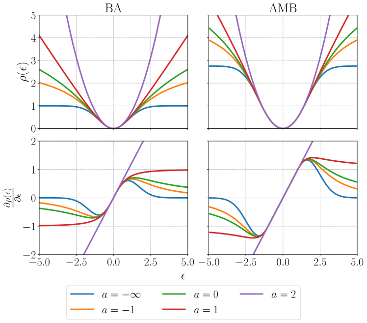
Figure 14: The general loss function by [5] (BA) and its gradient are shown in the left column for different values of its shape parameter ${\alpha}$. The right column shows the AMB loss function and its gradient for the mode ${\tilde{\epsilon}=1}$.

Appendix C Outlier Process Function for AGNC

Recall the surrogate function of (10) is

$$\rho_{\mu}(\epsilon,\alpha^{\star}) =\frac{\left|f-2\right|}{f}\left(\left(\frac{\epsilon^{2}}{\left|f-2\right|}+1\right)^{\nicefrac{{f}}{{2}}}-1\right),$$ (75)

where ${f=f(\mu,\alpha^{\star})}$ is the shape function. Substituting (75) into (59), differentiating both sides with respect to ${\epsilon}$, and isolating ${\phi^{\prime}(\cdot)}$ results

$$2\epsilon\phi^{\prime}_{\mu}\left(\epsilon^{2},\alpha^{\star}\right) =\rho^{\prime}_{\mu}\left(\epsilon,\alpha^{\star}\right)$$ (76)

$$=\epsilon\left(\frac{\epsilon^{2}}{\left|f-2\right|}+1\right)^{\nicefrac{{f}}{{2}}-1},$$ (77)

$$\phi^{\prime}_{\mu}\left(\epsilon^{2},\alpha^{\star}\right) =\mbox{$\textstyle{\frac{1}{2}}$}\left(\frac{\epsilon^{2}}{\left|f-2\right|}+1\right)^{\nicefrac{{f}}{{2}}-1}.$$ (78)

Moreover, differentiating ${\phi^{\prime}_{\mu}}$ with respect to ${\epsilon^{2}}$ yields

$$\phi^{\prime\prime}_{\mu}\left(\epsilon^{2},\alpha^{\star}\right)=\frac{1}{4}\frac{f-2}{\left|f-2\right|}\left(\frac{\epsilon^{2}}{\left|f-2\right|}+1\right)^{\nicefrac{{f}}{{2}}-2}.$$ (79)

Note that the functions in (78) and (79) satisfy the sufficient conditions,

$$\lim_{\epsilon^{2}\to{0}}\phi^{\prime}_{\mu}\left(\epsilon^{2},\alpha\right)=\mbox{$\textstyle{\frac{1}{2}}$}, \quad\forall f<2,$$ (80)

$$\lim_{\epsilon^{2}\to{\infty}}\phi^{\prime}_{\mu}\left(\epsilon^{2},\alpha\right)=0, \quad\forall f<2,$$

$$\phi^{\prime\prime}_{\mu}\left(\epsilon^{2},\alpha\right)<0, \quad\forall f<2.$$

The inverse function in (66) is

$$\left(\phi^{\prime}_{\mu}\right)^{-1}\left(\mbox{$\textstyle{\frac{1}{2}}$}w\right)=\left|f-2\right|\left(w^{\nicefrac{{2}}{{(f-2)}}}-1\right).$$ (81)

Then, the outlier process function can be computed using (67),

$$\Phi_{{\rho}_{\mu}} =\frac{\left|f-2\right|}{f}\left(w^{\nicefrac{{f}}{{(f-2)}}}-1\right)-w\frac{\left|f-2\right|}{2}\left(w^{\nicefrac{{2}}{{(f-2)}}}-1\right).$$ (82)

References

- [1] Cesar Cadena et al. “Past, present, and future of simultaneous localization and mapping: Toward the robust-perception age” In IEEE Transactions on Robotics 32, 2016, pp. 1309–1332 DOI: 10.1109/TRO.2016.2624754
- [2] Peter J Huber “Robust estimation of a location parameter” In The Annals of Mathematical Statistics 35 Institute of Mathematical Statistics, 1964, pp. 73–101 URL: http://www.jstor.org/stable/2238020
- [3] Michael Black and Padmanabhan Anandan “The robust estimation of multiple motions: Parametric and piecewise-smooth flow fields” In Computer Vision and Image Understanding 63, 1996, pp. 75–104 DOI: 10.1006/cviu.1996.0006
- [4] Donald Geman and Stuart Geman “Bayesian image analysis” In Disordered Systems and Biological Organization Springer Berlin Heidelberg, 1986, pp. 301–319
- [5] Jonathan T. Barron “A general and adaptive robust loss function” In Proceedings of the IEEE Computer Society Conference on Computer Vision and Pattern Recognition 2019-June IEEE Computer Society, 2019, pp. 4326–4334 DOI: 10.1109/CVPR.2019.00446
- [6] Nived Chebrolu et al. “Adaptive robust kernels for non-linear least squares problems” In IEEE Robotics and Automation Letters 6 Institute of ElectricalElectronics Engineers Inc., 2021, pp. 2240–2247 DOI: 10.1109/LRA.2021.3061331
- [7] Thomas Hitchcox and James Richard Forbes “Mind the gap: Norm-aware adaptive robust loss for multivariate least-squares problems” In IEEE Robotics and Automation Letters 7 Institute of ElectricalElectronics Engineers Inc., 2022, pp. 7116–7123 DOI: 10.1109/LRA.2022.3179424
- [8] Heng Yang, Pasquale Antonante, Vasileios Tzoumas and Luca Carlone “Graduated non-convexity for robust spatial perception: From non-minimal solvers to global outlier rejection” In IEEE Robotics and Automation Letters 5 Institute of ElectricalElectronics Engineers Inc., 2020, pp. 1127–1134 DOI: 10.1109/LRA.2020.2965893
- [9] Michael J Black and Anand Rangarajan “On the unification of line processes , outlier rejection , and robust statistics with applications in early vision” In International Journal of Computer Vision 19, 1996, pp. 57–91
- [10] Rick Chartrand and Wotao Yin “Iteratively reweighted algorithms for compressive sensing” In IEEE International Conference on Acoustics, Speech and Signal Processing, 2008, pp. 3869–3872 DOI: 10.1109/ICASSP.2008.4518498
- [11] Andrew Blake and Andrew Zisserman “Visual Reconstruction” The MIT Press, 1987 DOI: 10.7551/mitpress/7132.001.0001
- [12] John E Dennis and Roy E Welsch “Techniques for nonlinear least squares and robust regression” In Communications in Statistics - Simulation and Computation 7, 1978, pp. 345–359
- [13] Philippe Babin, Philippe Giguère and François Pomerleau “Analysis of robust functions for registration algorithms” In IEEE International Conference on Robotics and Automation (ICRA) abs/1810.0, 2019, pp. 1451–1457 DOI: 10.1109/ICRA.2019.8793791
- [14] François Pomerleau, M Liu, Francis Colas and Roland Siegwart “Challenging data sets for point cloud registration algorithms” In International Journal of Robotics Research 31, 2012, pp. 1705–1711 DOI: 10.1177/0278364912458814
- [15] Jonathan Arsenault and James Richard Forbes “Practical considerations and extensions of the invariant extended Kalman filtering framework”, 2020, pp. 114
- [16] Y Chen and G Medioni “Object modeling by registration of multiple range images” In IEEE International Conference on Robotics and Automation (ICRA) 3 IEEE, 1991, pp. 2724–2729 DOI: 10.1109/ROBOT.1991.132043
- [17] P J Besl and Neil D McKay “A method for registration of 3D shapes” In IEEE Transactions on Pattern Analysis and Machine Intelligence 14, 1992, pp. 239–256 DOI: 10.1109/34.121791
- [18] Heng Yang and Luca Carlone “Certifiably Optimal Outlier-Robust Geometric Perception: Semidefinite Relaxations and Scalable Global Optimization” In IEEE Transactions on Pattern Analysis and Machine Intelligence 45 IEEE Computer Society, 2023, pp. 2816–2834 DOI: 10.1109/TPAMI.2022.3179463
- [19] Roman Kaskman, Sergey Zakharov, Ivan Shugurov and Slobodan Ilic “HomebrewedDB: RGB-D dataset for 6D pose estimation of 3D objects” In International Conference on Computer Vision (ICCV) Workshops, 2019
- [20] Qian-Yi Zhou, Jaesik Park and Vladlen Koltun “Open3D: A modern library for 3D data processing”, 2018
DeMenezes2021 \missingNeira2001 \missingRoysdon2017