Deep Finite Volume Method for Partial Differential Equations

Abstract

In this paper, we propose the deep finite volume method (DFVM), a novel deep learning method for solving partial differential equations (PDEs). The key idea is to design a new loss function based on the local conservation property over the so-called control volumes, derived from the original PDE. Since the DFVM is designed according to a weak instead of strong form of the PDE, it may achieve better accuracy than the strong-form-based deep learning method such as the well-known PINN, when the to-be-sloved PDE has an insufficiently smooth solution. Moreover, since the calculation of second-order derivatives of neural networks has been transformed to that of first-order derivatives which can be implemented directly by the Automatic Differtiation mechanism(AD), the DFVM usually has the computational cost much lower than that of the methods which need to compute second order derivatives by the AD. Our numerical experiments show that comparing to some deep learning methods in the literature such as the PINN, DRM and WAN, the DFVM obtains same or higher accurate approximate solutions by consuming significantly lower computational cost. Moreover, for some PDE with a non smooth solution, the relative error of approximate solutions by DFVM is two-orders-of-magnitude less than that by the PINN.

1 Introduction

Partial differential equations (PDEs) are prevalent and extensively applied in science, engineering, economics, and finance. Traditional numerical methods, such as, the finite difference method [19], the finite element method [42], and the finite volume method [37] have achieved great success in solving PDEs. However, for some nonlinear or high dimensional PDEs, or PDEs with complex geometry, there are significant challenges for traditional methods (see reference [6]). For instance, a traditional numerical method often suffers from the so-called curse of dimensionality in the sense that the number of unknowns grows exponentially as the dimension increases. Recently, deep learning methods gain a lot of popularity in solving PDEs due to its simplicity and flexibility [34, 6, 41, 21, 20].

A deep learning method often simulates the solution of a PDE by training a neural network’s parameters according to some deliberately designed loss. There are two different types of loss. The first type of loss is designed directly according to the so-called strong form of the PDE and its initial/boundary conditions. Precisely, this type of loss is designed based on the residuals of the PDE in the least square sense. Note that the loss of the well-known PINN([30]) belongs to this type. For their simplicity and elegance, the deep solvers with this type of loss have been widely applied to various problems such as the Schrödinger equation [9], the Hamilton Jacobi-Bellman equations [7], the nonlinear Black-Scholes equation [3], as well as problems with random uncertainties [40, 41]. The second type of loss is designed according to some weak forms of the original PDE. For instances, the loss of the deep Ritz method (DRM,[6]) is designed according to the minimization of an energy functional; the loss of the weak adversarial networks (WAN, [38]) is designed according to the saddle-point problem induced by the weak formulation of the original PDE; the deep mixed residual method (MIM, [23]) designed its loss by transforming the original PDE to lower order PDEs.

An apparent difference between the above two types of loss is: by the loss of first type, one often needs to calculate high-order (same as the order of the original PDE) derivatives of the to-be-trained neural network, while by the loss of second type, one only needs to calculate some lower order (lower than the order of the original PDE) derivatives of the to-be-trained neural network. For instance, to solve a second-order PDE, the loss of the PINN involves the second-order derivatives terms, while the loss of the DRM([6]) only involves first-order derivatives terms. Recall that in the deep-learning related calculus, the first-order derivative of a neural network function is often implemented by a so-called Automatic Differentiation mechanism (AD,[32, 1]), which is very effective and powerful to calculate first-order derivatives since the calculation of first-order derivatives only needs one time reverse-pass operation after the forward-pass operation for calculating the function value of the neural network has been completed. However, to calculate second-order derivatives, one needs to apply first-order AD $d+1$ times, and thus the cost will increase significantly along with the dimension $d$ ([22]). In the following, we use a specific example to quantify the change of cost by AD to compute derivatives of a network function. Precisely, we test on a function $u_{\theta}:\mathbb{R}^{d}\to\mathbb{R}$ which is actually a fully connected network containing 6 hidden layers and 200 neurons per layer. Listed in Table 1 are computing time for computing $u_{\theta},\nabla u_{\theta}$, and $\Delta u_{\theta}$ 1000 times for each of 1000 random sampling points in $\mathbb{R}^{d}$ using a computer equipped with NVIDIA TITAN RTX. We observe that the computational cost of first-order derivatives is roughly similar at different dimensions, while the cost of $\Delta u_{\theta}$ increases significantly along with the dimension. Since the training of a deep PDE solver often takes many times’ calculation of the loss and its derivative (with respect to weights) on a large amount of sampling points, the above fact implies that for solving a high dimensional PDE, one should try to avoid calculating second or more higher order derivatives of a network directly using the AD.

Table 1: Computation time by the AD.

dim	$u_{\theta}$	$\nabla u_{\theta}$	$\Delta u_{\theta}$
2	0.52s	0.41s	2.32s
10	0.58s	0.42s	10.81s
50	0.67s	0.44s	53.66s
100	0.75s	0.50s	110.20s
200	0.77s	0.54s	219.40s

Next we illustrate the idea to compute $\Delta u_{\theta}({\bf x}_{0}),{\bf x}_{0}\in\mathbb{R}^{d}$ without directly using the AD twice. Let $V$ be some volume (e.g cube or ball) surrounding ${\bf x}_{0}$. When the size of $V$ is sufficiently small, we can use the average $\frac{1}{|V|}\int_{V}\Delta u_{\theta}dx$ to approximate $\Delta u_{\theta}({\bf x}_{0})$. On the other hand, by the divergence theorem ([26]),

(1) $$\int_{V}\Delta u_{\theta}d{\bf x}=\int_{\partial V}\frac{\partial u_{\theta}}{\partial{\vec{n}}}ds,$$

where $\vec{n}$ is the unit outward normal. Using a proper quadrature to calculate the right hand side’s integral of (1), we obtain a scheme

(2) $$\Delta u_{\theta}({\bf x}_{0})\approx\frac{1}{|V|}\sum_{{\bf y}_{j}\in\partial V}c_{j}\frac{\partial u_{\theta}}{\partial{\vec{n}}}({\bf y}_{j}),$$

where $c_{j},{\bf y}_{j}$ are weights and locations depending on the selected quadrature. We will give a detailed construction of (2) in our main text and simply highlight here that (2) is different from a traditional difference scheme by which $\Delta u_{\theta}({\bf x}_{0})$ is calculated with a linear combination of the function $u_{\theta}$ valued at several different locations, since here by (2), $\Delta u_{\theta}({\bf x}_{0})$ is calculated with the first order derivatives of $u_{\theta}$ valued at different locations.

The above strategy to simulate $\Delta u_{\theta}$ with first-order derivatives can be extended to any other second-order derivatives, therefore we actually have proposed a novel method to design the loss for solving general second-order PDEs. Moreover, since any high-order derivatives of a network function can be similarly simulated by its one-order lower derivatives, the above strategy actually proposes a novel loss for solving any high-order PDEs. Since the above method depends on the volumes associated with the finite number of training points, we called this method as the deep finite volume method(DFVM). It may be worth mentioning that unlike the traditional finite volume method where all control volumes constitute a partition of the domain $\Omega$, all control volumes of a DFVM are not necessary to constitute a partition of $\Omega$.

Therefore, DFVM reduces the computational cost and obtains more accurate approximate solutions. Compared with other deep learning solvers for PDEs, the DFVM enjoys higher feasibility in two aspects: First, the use of the weak formulation makes it more feasible to solve general high dimensional PDEs defined on arbitrarily shaped domains. Second, DFVM also works well for asymmetric problems and non-homogeneous boundary problems, which the DRM can not handle well. In addition, DFVM preserves physical conservation property in a control volume associated with each sampling point, which is also not available in other existing deep learning methods.

It is worth mentioning that DFVM not only reduces the computational cost but also obtains more accurate approximate solutions. Our numerical results show that, for high-dimensional linear and nonlinear elliptic PDEs, DFVM provides better approximations than DGM and WAN with nearly the same DNN and the same execution time, by one order of magnitude. The relative error obtained by DFVM is slightly smaller than that obtained by PINN, while the computation cost of DFVM is an order of magnitude less than that of the PINN. For the time-dependent Black-Scholes equation, DFVM gives better approximations than PINN, by one order of magnitude.

The approximation of the derivatives obtained by the difference scheme is inherently ill-conditioned and unstable. In this work, we will introduce the finite volume method which enjoys good properties such as numerical stability and flexibility in handling geometric domains to transform the second derivatives of neural network functions to first-order derivatives, then we use AD to obtain first-order derivatives in our new DFVM.

The rest of the paper is organized as follows. In Section 2, we introduce the neural network architecture used in this paper. In Section 3, we introduce DFVM for high-dimensional PDEs. Numerical results for four types of PDEs are provided to illustrate the performance of DFVM in Section 4. A brief Conclusion and discussion are drawn in Section 5.

2 The deep finite volume method(DFVM)

In this section, we present the deep finite volume method (DFVM) for solving the following partial differential equation

(3) $$\mathcal{L}u =f\quad\text{in}~{}\Omega$$

(4) $$\mathcal{B}u =g\quad\text{on}~{}\partial\Omega,$$

where $\Omega$ is a bounded domain in $\mathbb{R}^{d}$ with boundary $\partial\Omega$, ${\cal L}$ and ${\cal B}$ are some given interior and boundary differential operators, respectively.

The main purpose of this section is to train a neural network $u_{\theta}$ to approximate the exact solution $u$ of the problem (3)-(4). Without loss of generality, we choose $u_{\theta}$ as a ResNet type network which takes the form

(5) $$u_{\theta}({\bf x})=({\bf B}_{l+1}\circ{\bf B}_{l}\circ{\bf B}_{l-2}\circ\cdots\circ{\bf B}_{2}\ \circ{\bf B}_{0})({\bf x}),\ {\bf x}\in\mathbb{R}^{d},$$

where each residual block is presented as

$${\bf B}_{k}=\sigma({\bf W}_{k}\sigma({\bf W}_{k-1}{\bf B}_{k-2})+{\bf b}_{k-1})+{\bf b}_{k})+{\bf B}_{k-2},\ k=2,4,\cdots,l.$$

and

$${\bf B}_{0}=\sigma({\bf W}_{0}x+{\bf b}_{0}),\ {\bf B}_{l+1}=\sigma({\bf W}_{l+1}{\bf B}_{l}+{\bf b}_{l+1}).$$

Here, $\sigma$ is the activation function and $\boldsymbol{\theta}=\left\{{\bf W}_{k},{\bf b}_{k},|k=0,1,\cdots,l+1\right\}$ are parameters to be trained.

Before illustrating on how to train $u_{\theta}$, we first introduce the basic idea on how to solve partial differential equations with a classic finite volume method.

2.1 Quadratures over control volumes and their boundaries

For simplicity, we choose a control volume(CV) in the DFVM as a cube or ball in $\mathbb{R}^{d}$. Precisely, given a point ${\bf x}_{0}=(x^{1}_{0},\ldots,x^{d}_{0})\in\mathbb{R}^{d}$ and a size quantity $h>0$, we let $V_{{\bf x_{0}},h}$ be the $d$-dimensional cube

$$V_{{\bf x_{0}},h}=\prod\limits_{j=1}^{d}[x^{j}_{0}-h,x^{j}_{0}+h],$$

or the $d$-dimensional ball

$$V_{{\bf x_{0}},h}=\{{\bf x}=(x^{1},\ldots,x^{d})\in\mathbb{R}^{d}\mid\sum_{j=1}^{d}(x^{j}-x^{j}_{0})^{2}\leq h^{2}\}.$$

Normally, we choose $V_{{\bf x_{0}},h}$ as a cube when $d\leq 3$ and a ball when $d\geq 4$. Noticing that $V_{{\bf x_{0}},h}$ is not necessary in the interior of $\Omega$, the actual CV is often chose as $V=V_{{\bf x_{0}},h}\cap\Omega$, the part of $V_{{\bf x_{0}},h}$ in $\Omega$.

Next we illustrate how to numerically calculate an integral over $V$ or $\partial V$, the boundary of $V$. Let $Q_{r}(F)=\sum_{j=1}^{r}w_{j}F(g_{j}),r\geq 1$ be the $r$th order Gauss quadrature to calculate the integral $\int_{-1}^{1}f(x)dx$, where $-1\leq g_{1}<\ldots<g_{r}\leq 1$ are $r$ Gauss points and $w_{j},1\leq j\leq r$ are corresponding weights. By an affine transformation, we can use the quadrature

$$Q_{r}(F,[a,b])=\frac{(b-a)}{2}\sum_{j=1}^{r}w_{j}F(g^{[a,b]}_{j}),g_{j}^{[a,b]}=\frac{a+b}{2}+\frac{b-a}{2}g_{j},1\leq j\leq r$$

to calculate the 1D integral $\int_{a}^{b}Fdx$. Noticing that an interval $[a,b]$ is uniquely determined by its center $c=\frac{a+b}{2}$ and half length $\hat{h}=\frac{b-a}{2}$, so sometimes, we also denote $Q_{r}(F,c,\hat{h})=Q_{r}(F,[a,b])$ and $g_{j}^{c,\hat{h}}=g_{j}^{[a,b]},1\leq j\leq r$. With this notation, a Gauss quadrature on a $d$-dimensional control volume $V=V_{{\bf x_{0}},h}$ can be presented as

$$Q_{r}(F,V_{{\bf x_{0}},h})=h^{d}\sum_{j_{1},\ldots,j_{d}=1}^{r}w_{j_{1}}\cdots w_{j_{d}}F(g_{j_{1}}^{x_{0}^{1},h},\ldots,g^{x^{j}_{0},h}_{j_{i}},\ldots,g_{j_{d}}^{x^{d}_{0},h}),$$

which can be used to calculate the integral $\int_{V_{{\bf x_{0}},h}}Fd{\bf x}$. Next, we present quadratures for the integral on the boundary $\partial V$. In the case $d=2$, $\partial V$ is the union of 4 segments and thus

(6) $$\int_{\partial V}Fds\approx Q_{r}(F,\partial V) = Q_{r}(F(x^{1}_{0}+h,\cdot),x^{2}_{0},h)+Q_{r}(F(x^{1}_{0}-h,\cdot),x^{2}_{0},h))$$

$$+Q_{r}(F(\cdot,x^{2}_{0}+h),x^{1}_{0},h)+Q_{r}(F(x^{2}_{0}-h,\cdot),x^{1}_{0},h).$$

In the case $d=3$, $\partial V$ is the union of 6 squares, therefore

(7) $$\int_{\partial V}Fds\approx Q_{r}(F,\partial V) = Q_{r}(F(x^{1}_{0}+h,\cdot,\cdot),S_{1})+Q_{r}(F(x^{1}_{0}-h,\cdot,\cdot),S_{1})+Q_{r}(F(\cdot,x^{2}_{0}+h,\cdot),S_{2})$$

$$+Q_{r}(F(\cdot,x^{2}_{0}-h,\cdot),S_{2})+Q_{r}(F(\cdot,\cdot,x^{3}_{0}+h),S_{3})+Q_{r}(F(\cdot,\cdot,x^{3}_{0}-h,\cdot),S_{3}),$$

where $S_{1}=[x^{2}_{0}-h,x^{2}_{0}+h]\times[x^{3}_{0}-h,x^{3}_{0}+h],S_{2}=[x^{1}_{0}-h,x^{1}_{0}+h]\times[x^{3}_{0}-h,x^{3}_{0}+h],S_{3}=[x^{1}_{0}-h,x^{1}_{0}+h]\times[x^{2}_{0}-h,x^{2}_{0}+h]$.

When $d>3$, we choose the volume $V_{{\bf x}_{0},h}$ to be the ball centered at ${\bf x}_{0}$ with the radius $h$. For this high dimensional case, we prefer to use the (quasi) Monte-Carlo method to calculate the integrals $\int_{V}F$ and $\int_{\partial V}F$. Fixing two positive integers $J_{V}$ and $J_{\partial V}$ which are independent of the dimension $d$, we randomly sample $J_{V}$ points ${\bf x}_{j},j=1,\ldots,J_{V}$ from the interior of $V$ and $J_{\partial V}$ points ${\bf y}_{j},j=1,\ldots,J_{\partial V}$ from the boundary $\partial V$. We denote $S_{V}:=\{{\bf x}_{j}\in V|j=1,\ldots,J_{V}\}$ and $S_{\partial V}:=\{{\bf y}_{j}\in\partial V|j=1,\ldots,J_{\partial V}\}$ as the set of training points in $V$ and $\partial V$ respectively. Then we use the quadrature (see [2, 4])

(8) $$\int_{\partial V}Fds \approx Q_{MC}(F,V)=\frac{|V|}{J_{V}}\sum_{{\bf x}\in S_{V}}F({\bf x}),$$

and

(9) $$\int_{\partial V}Fds \approx Q_{MC}(F,\partial V)=\frac{|\partial V|}{J_{\partial V}}\sum_{{\bf x}\in S_{\partial V}}F({\bf x}).$$

Remark that we may choose the number $J_{V}$ and $J_{\partial V}$ to be independent of the dimension $d$, so that the computational cost of quadratures (8) and (9) is also independent of the dimension $d$.

In summary, we let the quadrature

$$Q(F,V)=\left\{\begin{array}[]{ll}Q_{r}(F,V),&d\leq 3\\ Q_{MC}(F,V),&d\geq 4\end{array}\right.\ {\rm and}\ \ Q(F,\partial V)=\left\{\begin{array}[]{ll}Q_{r}(F,\partial V),&d\leq 3\\ Q_{MC}(F,\partial V),&d\geq 4.\end{array}\right.$$

2.2 Loss

In this subsection, we illustrate how to construct the loss of the DFVM for solving PDEs.

2.2.1 Divergence-form second-order PDEs

We begin with the case that $\mathcal{L}$ in (3) is a divergence-form second-order operator given by

(10) $$\mathcal{L}u=-\nabla\cdot\left(\mathbf{A}\nabla u\right)+{\bf b}\cdot\nabla u+cu,$$

where both the matrix ${\bf A}$ and vector ${\bf b}$ are known variable-coefficients. The boundary condition(s) in (4) can be Dirichlet, Neumann and Robin types. We suppose that the coefficient matrix ${\bf A}=(a_{ij}(x):1\leq i,j\leq d)$ is symmetric, uniformly bounded and positive definite in the sense that there exist positive constants $\alpha,\beta$ such that

$$\alpha\xi^{t}\xi\leq\xi^{t}A(x)\xi\leq\xi^{t}\xi,\forall x\in\Omega,\xi\in\mathbb{R}^{d}.$$

Note that under the above properties on ${\bf A}$ and some appropriate properties on ${\bf b}$ and $c$, the corresponding PDE (3) and (4) has a unique solution.

As in a standard deep PDE solver, the loss of the DFVM will be designed in a least square sense. Let ${\cal S}_{int}$ be the set of training points sampled from the interior of $\Omega$ according to a certain distribution(e.g. the Uniform or the Gaussian distribution). Fixing a size $h>0$, we establish a control volume(CV) $V=V_{{\bf x},h}\cap\Omega$ for each point ${\bf x}\in S_{int}$. We have

$$\int_{V}\big{(}\mathcal{L}u_{\theta}-f{\rm\ }\big{)}dV =\int_{V}\big{(}-\nabla\cdot\left(\mathbf{A}\nabla u_{\theta}\right)+{\bf b}\nabla u_{\theta}+cu_{\theta}-f\big{)}dV$$

(11) $$=-\int_{\partial V}\left(\mathbf{A}\nabla u_{\theta}\right)\cdot{\vec{n}}dS+\int_{V}\left({\bf b}\nabla u_{\theta}+cu_{\theta}-f\right)dV,$$

where ${\vec{n}}$ is the unit normal outward $V$, and in the second equality, we have used the divergence theorem([26]) to transform an integral in a volume to an integral on its boundary surface.

The interior loss is then defined by

(12) $$\mathcal{J}^{int}(u_{\theta})=\frac{1}{\#{\cal S}_{int}}\sum_{{\bf x}\in{\cal S}_{int}}\frac{1}{|V|^{2}}\big{|}Q(\left(-\mathbf{A}\nabla u_{\theta}\right)\cdot{\vec{n}},\partial V)+Q({\bf b}\cdot\nabla u_{\theta}+cu_{\theta}-f,V)\big{|}^{2}.$$

We emphasize that in the loss (12), no second order derivative term is involved.

Similarly, Let ${\cal S}_{bdy}$ be the set of training points sampled from the boundary $\partial\Omega$ according to a certain distribution, we define the boundary loss as

(13) $$\mathcal{J}^{bdy}(u_{\theta})=\frac{1}{\#{\cal S}_{bdy}}\sum_{{\bf x}\in{\cal S}_{bdy}}\left|\mathcal{B}u_{\theta}({\bf x})-g({\bf x})\right|^{2}.$$

The total loss function is then defined by

(14) $$\mathcal{J}(u_{\theta})=\mathcal{J}^{int}(u_{\theta})+\lambda\mathcal{J}^{bdy}(u_{\theta}),$$

where $\lambda$ is some parameter to be determined.

2.2.2 General second-order PDEs

In this subsection, we discuss how to design the loss for the case that $\mathcal{L}$ in (3) is a general second-order operator given by

(15) $$\mathcal{L}u=-\mathbf{A}:D^{2}u+{\bf b}\cdot\nabla u+cu,$$

where the tensor product

$${\bf A}:D^{2}v=\sum_{1\leq i,j\leq d}a_{ij}\partial^{2}_{x_{i}x_{j}}v,\forall v\in H^{2}(\Omega).$$

In addition, we often assume that the coefficient tensor ${\bf A}$ satisfies the Cordes condition; that is, there exists an $\epsilon\in[0,1]$ such that

$$\frac{|{\bf A}|^{2}}{(tr{\bf A})^{2}}\leq\frac{1}{(d-1+\epsilon)},$$

where $|{\bf A}|^{2}=\sum_{i,j=1}^{d}a^{2}_{ij}.$ Note that the Cordes condition is often necessary ([35]) to ensure that the original PDE has a unique solution.

If the coefficient matrix ${\bf A}\in[C^{1}(\Omega)]^{d\times d}$, then the operator ${\cal L}$ can be rewritten as the divergence form

(16) $$\mathcal{L}u=-\nabla\cdot\left(\mathbf{A}\nabla u\right)+(\nabla\cdot{\bf A}+{\bf b})\cdot\nabla u+cu,$$

so that we can design the loss according to the method presented in Section 2.2.1. In the case ${\bf A}\notin[C^{1}(\Omega)]^{d\times d}$, we does not have the above global transformation to allow us to transform the integral of all second order derivative terms on a volume to the integral of first order derivative terms on the boundary of the volume only by once. Fortunately, we can use the fact that

$$\partial^{2}_{x_{i},x_{j}}u={\rm div}{\bf v}$$

where ${\bf v}=(v_{1},\ldots,v_{d})$ is a vector given by

$$v_{k}=\left\{\begin{array}[]{ll}0,&k\not=i,\\ \frac{\partial u}{\partial x_{j}},&k=i,\end{array}\right.$$

to transform the integral

$$\int_{V_{{\bf x},h}}\alpha_{ij}\partial^{2}_{x_{i},x_{j}}u_{\theta}d{\bf x}\approx\alpha_{ij}({\bf x})\int_{\partial V_{{\bf x},h}}{\bf v}\cdot\vec{n}ds=\alpha_{ij}({\bf x})\int_{\partial V_{{\bf x},h}}\frac{\partial u_{\theta}}{\partial x_{j}}n_{i}ds,$$

where $n_{i},1\leq i\leq d$ is the $i$th component of the normal vector ${\vec{n}}$. Then the interior loss is defined by

(17) $$\mathcal{J}^{int}(u_{\theta})=\frac{1}{\#{\cal S}_{int}}\sum_{{\bf x}\in{\cal S}_{int}}\frac{1}{|V|^{2}}\big{|}\sum_{i,j=1}^{d}\alpha_{ij}({\bf x})Q(\frac{\partial u_{\theta}}{\partial x_{j}}n_{i},\partial V)+Q({\bf b}\cdot\nabla u_{\theta}+cu_{\theta}-f,V)\big{|}^{2}.$$

2.2.3 High order PDEs

If ${\cal L}$ is a differential operator of order higher than 2, we may use some so-called mid-variables to transform (3) to a system of second order equations. For instances, when ${\cal L}u=\Delta^{2}u$, we introduce the mid-variable $v=\Delta u$ to transform the biharmonic equation

(18) $$\Delta^{2}u=f$$

a system of two second-order equations as below

(19) $$\Delta u=v\ \ {\rm in}\ \ \Omega,$$

(20) $$\Delta v=f\ \ {\rm in}\ \ \Omega.$$

When ${\cal L}u=\frac{\partial u}{\partial t}+\varepsilon^{2}\Delta^{2}u-\Delta\left(u^{3}-u\right)$ is the fourth order Cahn-Hilliard type operator, we may use the mid-variable $v=-\varepsilon^{2}\Delta u+u^{3}-u$ to transform the Cahn-Hilliard equation

(21) $$\frac{\partial u}{\partial t}=-\varepsilon^{2}\Delta^{2}u+\Delta\left(u^{3}-u\right)+g,$$

to the system of second order equations

(22) $$\varepsilon^{2}\Delta u =-v+u^{3}-u,$$

(23) $$\Delta v =\frac{\partial u}{\partial t}-g.$$

When ${\cal L}u=\frac{\partial u}{\partial t}-\Delta\left[u^{2}+u^{3}+\left(\left(q_{0}+\Delta\right)^{2}-\varepsilon\right)u\right]$ is the sixth order Phase-Field Crystal operator, we may use the mid-variables $v=q_{0}u+\Delta u,w=u^{2}+u^{3}-\varepsilon u+(q_{0}+\Delta)v$ to transform the Phase-Field Crystal equation

(24) $$\frac{\partial u}{\partial t}=\Delta\left[u^{2}+u^{3}+\left(\left(q_{0}+\Delta\right)^{2}-\varepsilon\right)u\right],$$

where $q_{0}$ and $\varepsilon$ are constants, to the system of three second-order equations as

(25) $$(q_{0}+\Delta)u =v,$$

(26) $$(q_{0}+\Delta)v =w-u^{2}-u^{3}+\varepsilon u,$$

(27) $$\Delta w =\frac{\partial u}{\partial t}.$$

2.3 The adaptive trajectories sampling DFVM(ATS-DFVM)

In the previous section, we train the parameters of a neural network solution on fixed training points. In this section, we explain how to update the set of training points adaptively according to the computed approximate solution to improve the performance of a deep learning solver for PDEs.

We recall that the adaptive selection of training points is an important tool to improve the performance of a deep solver of PDEs. Along this direction, a lot of effort has been put into, see e.g. [22, 25, 8, 39, 36] for an uncompleted list of publications. In this paper, we illustrate how to apply a novel adaptive sampling technique, which is called as ATS and is developed in [5] very recently, to the DFVM to improve the performance. Without loss of generality, in the following we only explain how to adaptively generate the interior-training-points set ${\cal S}_{int}$ of which the cardinality will be fixed to be some given positive number $I$. In the very beginning, the set ${\cal S}_{int}$ is obtained by randomly sampling in the interior of $\Omega$ according to a certain distribution. Then after a period of training using the points in ${\cal S}_{int}$, we update the points in ${\cal S}_{int}$ as below. For each ${\bf x}_{i}\in{\cal S}_{int},1\leq i\leq I$, we use the Gaussian stochastic process to generate $J$ novel points. Precisely, we let

(28) $$\mathbf{x}_{i,j}=\mathbf{x}_{i}+\sqrt{\Delta t}\mathcal{N}\left(0,\mathcal{I}_{d}\right),j=1,\ldots,J,$$

where $\Delta t>0$ is a small prescribed radius and $\mathcal{N}$ is the normalized Gauss process. We define the next step’s set of candidate training points as

$${\mathcal{S}}^{\prime}_{int}=\{{\bf x}_{i,j}|1\leq i\leq I,1\leq j\leq J\}\cup{\mathcal{S}}_{int}.$$

To determine which point in the candidate set ${\mathcal{S}}^{\prime}_{int}$ will be chosen as a training point of the next training epoch, we construct an error indicator

(29) $${\rm Ind}_{V}({\bf x})=\big{|}Q(\left(-\mathbf{A}\nabla u_{\theta}\right)\cdot{\vec{n}},\partial V_{{\bf x},h})+Q({\bf b}\cdot\nabla u_{\theta}+cu_{\theta}-f,V_{{\bf x},h})\big{|}.$$

The set of training points in the next training epoch is then obtained by choosing the $I$ points in ${\mathcal{S}}^{\prime}_{int}$ at which the error indicator is bigger than that elsewhere. Namely, the novel set of training points ${\mathcal{S}}^{new}_{int}$ satisfies the following two properties : 1) $\#{\mathcal{S}}^{new}_{int}=I$, 2) ${\rm Ind}_{V}({\bf x})\geq{\rm Ind}_{V}({\bf y})$ for all ${\bf x}\in{\mathcal{S}}^{new}_{int},{\bf y}\in{\mathcal{S}}^{\prime}_{int}\setminus{\mathcal{S}}^{new}_{int}$.

3 Numerical experiments

In this section, we test the performance of the DFVM. First we compare the performance of the DFVM and the AD by applying them to calculate $\Delta u_{\theta}$, the Laplacian of a neural network function $u_{\theta}$. We found that with a proper chosen volume size ($h=10^{-5})$, the DFVM computes a very accurate approximation of $\Delta u_{\theta}$ by consuming far less time than that of the AD. Secondly, we apply the DFVM to solve variants of PDEs including the Poisson equation, the biharmonic equation, the Cahn-Hilliard equation, and the Black-Scholes equation.

In all our numerical experiments, the neural network will be chosen as the ResNet which has 3 blocks and 128 neurons per layer. And for all methods, we use Adam optimizer to train the network parameters. Moreover, unless otherwise specified, the activation function will be chosen as the tanh function. The accuracy of $u_{\theta}$ is indicated by the $L^{2}$ relative error defined by $\displaystyle{{\rm RE}=\|u_{\theta}-u\|_{L^{2}}/\|u\|_{L^{2}}}$. All numerical experiments except the final one are implemented using Python with the library Torch on a machine equipped with NVIDIA TITAN RTX GPUs, while the final one is computed with an Nvidia GeForce GTX 2080 Ti GPU.

3.1 Computing $\Delta u_{\theta}$ with the DFVM

In this subsection, we use the DFVM to calculate the second order derivative $\Delta u_{\theta}$ at 100 randomly chosen points in $R^{d}$ for variants of dimension $d$. Our to-be tested neural network function $u_{\theta}$ contains three residual blocks, with 128 neurons in each layer, and its activation function is chosen to be the tanh function. We initialize the weight parameters $\theta$ using a Gaussian distribution with a mean of 0 and a variance of 0.1.

We first test the accuracy of the DFVM-calculated $\Delta u_{\theta}$ in variants of cases. Precisely, we will test the cases that the dimension $d$ varies from $2$ to $100$ and the volume size $h$ varies from $10^{-1}$ to $10^{-10}$. Moreover, we fix $J_{V}$ and $J_{\partial V}$ to be 1 and $2*d$, respectively. Listed in Table 2 are the mean absolute errors (MAEs)[33] between the values of $\Delta u_{\theta}$ computed by the AD and that by the DFVM.

Table 2: MAEs of $\Delta u_{\theta}$ between the AD and the DFVM

$h$	d=2	d=10	d=20	d=40	d=60	d=80	d=100
1E-01	1.77E-03	4.67E-03	3.76E-03	3.23E-03	2.39E-03	2.43E-03	2.26E-03
1E-02	1.77E-05	4.69E-05	3.77E-05	3.24E-05	2.40E-05	2.43E-05	2.26E-05
1E-03	1.78E-07	4.69E-07	3.77E-07	3.24E-07	2.40E-07	2.43E-07	2.26E-07
1E-04	1.78E-09	4.69E-09	3.77E-09	3.24E-09	2.40E-09	2.43E-09	2.26E-09
1E-05	2.88E-11	6.86E-11	6.68E-11	9.45E-11	8.93E-11	9.35E-11	9.75E-11
1E-06	1.86E-10	4.51E-10	6.47E-10	8.59E-10	8.57E-10	9.75E-10	9.58E-10
1E-07	1.81E-09	4.80E-09	6.08E-09	8.10E-09	8.52E-09	1.06E-08	1.06E-08
1E-08	2.46E-08	4.48E-08	6.22E-08	7.96E-08	8.98E-08	1.03E-07	9.76E-08
1E-09	2.10E-07	4.99E-07	6.68E-07	7.86E-07	8.37E-07	9.41E-07	1.08E-06
1E-10	1.86E-06	4.41E-06	5.74E-06	8.10E-06	8.49E-06	1.07E-05	1.03E-05

From the above table, we observe that for all dimensions, the MAE first decreases and then increases as the radius $h$ decreases. This might be because that similarly to a difference method, theoretically, the smaller the $h$, the more accurate the DFVM-calculated value approximates the exact $\Delta u_{\theta}$, practically, along with the decrease of the size $h$, the accumulation error from floating-point arithmetic by the computer also increases. Therefore, the best approximation is often achieved when $h$ is neither too big nor too small. From Table 3.1, we observe that for all dimensions, the minimum MAE is achieved when the radius $h=10^{-5}$. Therefore, unless otherwise specified, we will set $h=10^{-5}$ for all subsequent numerical experiments in this section. Remark that when $h=10^{-5}$, the MAE between the approximate value by the DFVM and the exact $\Delta u_{\theta}$ achieves the order of $10^{-11}$, which is sufficiently accurate.

Next we compare the computational cost of the AD and DFVM. Recorded in Table 3.2 are computation time by using both methods to calculate $\Delta u_{\theta}$ 10,000 times over 100 randomly chosen testing points.

Table 3: Computation time by the DFVM and the AD

d	MAE	AD time(s)	DFVM time(s)
2	2.88E-11	36	12
4	3.13E-11	60	18
8	4.23E-11	105	24
10	6.86E-11	127	25
20	6.68E-11	265	47
40	9.45E-11	590	109
50	9.83E-11	614	118
60	8.93E-11	834	170
80	9.35E-11	1112	187
100	9.75E-11	1344	230

From this table, we find that for all dimensional cases, the consumed computing time of the DFVM is far less than that of the AD. In particular, for the cases $d=80,100$, the computation time by the DFVM is almost only $1/6$ of that by the AD, while the MAE achieves $10^{-11}$ which means that the approximate value of $\Delta u_{\theta}$ calculated by the DFVM is very accurate.

3.2 Solving PDEs with the DFVM

3.2.1 The Poisson equation

We consider the Poisson equation with Dirichlet boundary condition which has the following form

(30) $$-\Delta u=f\ {\rm in\ }\Omega,\ \ \ u=g\ {\rm on\ }\partial\Omega,$$

where $\Omega,f,g$ will be specified in the following three cases.

Case 1 In the first case, we let $\Omega=(0,1)^{2}\subset\mathbb{R}^{2}$, $f\equiv-2$ in $\Omega$ , and $g\left(x_{1},0\right)=g\left(x_{1},1\right)=x_{1}^{2}$ for $0\leq x_{1}\leq\frac{1}{2},g\left(x_{1},0\right)=g\left(x_{1},1\right)=\left(x_{1}-1\right)^{2}$ for $\frac{1}{2}\leq x_{1}\leq 1$, and $g\left(0,x_{2}\right)=g\left(1,x_{2}\right)=0$ for $0\leq x_{2}\leq 1$ on $\partial\Omega$. In this case, the problem (30) admits the solution

$$u^{*}(\mathbf{x})=u^{*}\left(x_{1},x_{2}\right)=\left\{\begin{array}[]{ll}x_{1}^{2},&0\leq x_{1}\leq\frac{1}{2},\\ \left(x_{1}-1\right)^{2},&\frac{1}{2}\leq x_{1}\leq 1,\end{array}\right.$$

which is continuous but nonsmooth.

We choose $u_{\theta}$ as a full-connected network which has 6 hidden layers, with 40 neurons per hidden layer. To train $u_{\theta}$, the number of internal points is set to be 10,000, and the number of boundary points is set to be 400. The weight of the boundary loss term is set to 1000. For the DFVM, we set the control volume radius h to 1e-3, $J_{V}=1$, $J_{\partial V}=4$. The optimizer used in each method is Adam with a learning rate of 0.001.

Listed in Table 4 are the $L^{2}$ relative errors (REs) between the exact solution and the approximate solution obtained from training 100,000 epochs by the PINN, DRM, and DFVM respectively. We find that for this case in which the exact solution is nonsmooth, the DFVM achieves much better accuracy with much less computation time than that by the PINN. To deepen impression, we depict the exact solution and the approximate solutions by the DFVM, the PINN, and the DRM in Figure 3.1. We find that the DFVM solution approximate the exact solution very closely, but the other two methods do not.

Table 4: REs and computation time of case 1 after 100,000 epochs

	RE	Time(s)
PINN	9.32E-01	1033
DRM	8.88E-01	615
DFVM	4.56E-03	600

(a) Exact solution

(b) DFVM solution

(c) PINN solution

(d) DRM solution

Fig. 1: The exact solution and approximate solution by different learning methods.

Case 2  In the second case, we let $\Omega=(0,1)^{d},f(x)=\displaystyle{\frac{1}{d}\left(\sin\left(\sum_{i=1}^{d}\frac{1}{d}x_{i}\right)-2\right)},g(x)=\displaystyle{\left(\sum_{i=1}^{d}\frac{1}{d}x_{i}\right)^{2}+\sin\left(\sum_{i=1}^{d}\frac{1}{d}x_{i}\right)}$. In this case, the solution of (30) is

$$u^{\ast}(x)=\left(\sum_{i=1}^{d}\frac{1}{d}x_{i}\right)^{2}+\sin\left(\sum_{i=1}^{d}\frac{1}{d}x_{i}\right).$$

In this case, the solution is sufficiently smooth. Our purpose is to test the dynamic change of the performance of the DFVM along with the dimension $d$. Precisely, we will use the DFVM to solve (30) for the dimensions $d=2,4,10,20,40,60,80,100,200$. For comparison, we will compute corresponding solutions by the PINN. We set the numbers of training points to be $\#\mathcal{S}_{int}=2000$, and $\#\mathcal{S}_{bdy}=100*d$. The weight of the boundary loss term is set to 1000.

Listed in Table (5) are the relative errors and computation time obtained from training $u_{\theta}$ 20000 epochs by the DFVM and the PINN. We observe that for all dimensional cases, the relative errors by both methods are of the same order, and the computation time of the DFVM is far less than that of the PINN.

Table 5: REs and computation time of case 2 after 20,000 epochs

	DFVM		PINN
d	RE	Time(s)	RE	Time(s)
2	1.76E-04	156	1.73E-04	321
4	2.33E-04	190	2.44E-04	465
8	4.60E-04	292	4.71E-04	934
10	6.77E-04	367	7.23E-04	984
20	1.91E-03	703	2.22E-03	2173
40	3.40E-03	1424	4.19E-03	3891
50	5.50E-03	1787	5.00E-03	4450
60	5.52E-03	2163	5.66E-03	5213
80	6.89E-03	3034	6.05E-03	5856
100	8.02E-03	3899	7.23E-03	6906
200	8.82E-03	8203	9.11E-03	12552

Case 3 In the third case, we let $\Omega=[-1,1]^{10}$ and the functions $f,g$ are chosen so that (30) admits the exact solution

(31) $$u(\mathbf{x})=e^{-10\|\mathbf{x}\|_{2}^{2}}.$$

Note that for this example, the solution $u=1$ at the origin and it decays very rapidly to zero as the location moves from the origin to the boundary of $\Omega$.

We choose $u_{\theta}$ as a fully connected neural network with 7 hidden layers and 20 neurons per layer, and we choose the activation function to be the tanh function. We will use three methods : the DFVM, the ATS-DFVM and the ATS-PINN to solve the equation (30) in this case. Note that in the initial stage of both the ATS-DFVM and the ATS-PINN, we randomly select 2000 interior points and 1000 boundary points to train 3000 epochs with the PINN method. After this initial stage, we resample the training points 10 times with ATS strategies, and after each resampling, we train the neural network 3000 epochs. The optimizer used in each method is Adam with a learning rate of 0.0001. For a fair comparison, the experiments in this case are implemented on a machine equipped with a V100 GPU.

We compute the DFVM, ATS-DFVM, ATS-PINN solution five times (with random seeds from 0 to 4). To measure the quality of approximation, we generate 10000 test points around the origin (in $[-0.1,0.1]^{d}$). The average relative errors and training times of five experiments are listed in Table 6.

Table 6: REs and computation time after 33,000 epochs.

	RE	Time(s)
DFVM	1.00E+00	465
ATS-DFVM	5.62E-02	605
ATS-PINN	3.82E-02	2323

From this table, we find that the DFVM solution is not a good approximation of the true solution. Actually, by checking our numerical results, we find that the DFVM solution is almost zero in the whole domain. One reason for this phenomenon might be that at almost all training points, which are sampled randomly according to the uniform distribution and thus away from the origin point, the true solution is very close to zero, therefore $u_{\theta}$, which is trained using these points, will be also almost zero. However, by the ATS techniques, the training points will gradually close to the origin point, see Figure 3.2. Consequently, we finally obtain a nice approximation of the true solution by the ATS-DFVM. From Table 3.2, we find that the ATS techniques can also improve the approximation accuracy of the PINN. However, the computational cost of the ATS-PINN is far more than that of the ATS-DFVM.

(a) 1st resampling

(b) 4th resampling

(c) 7th resampling

(d) 10th resampling

Fig. 2: ATS-DFVM training points in the $(x_{1},x_{2})$ plane. For display purpose, images only show the slices of $x_{3}=\cdots=x_{d}=0$.

3.2.2 High order PDEs

The biharmonic equation We consider

(32) $$\Delta^{2}u=f\ \ {\rm in}\ \ \Omega$$

with the boundary conditions

(33) $$u=\sum_{k=1}^{d}\text{sin}(\frac{\pi}{2}x_{k})\ \ {\rm on}\ \ \partial\Omega,$$

(34) $$\frac{\partial u}{\partial{\vec{n}}}=0\ {\rm on}\ \ \partial\Omega,$$

where $\Omega=[-1,1]^{2}$, and $\displaystyle{f=\frac{\pi^{4}}{16}\sum_{k=1}^{d}\text{sin}(\frac{\pi}{2}x_{k})}$. In this case, the exact solution is

(35) $$u({\bf x})=\sum_{k=1}^{d}\text{sin}(\frac{\pi}{2}x_{k}).$$

For this example, we choose $u_{\theta}$ as a full-connected network which has 4 hidden layers, with 40 neurons per hidden layer. To train $u_{\theta}$, the number of internal points is set to be 10,000, and the number of boundary points is set to be 800. The weight of the boundary loss term is set to 1000. For the DFVM, we set the control volume radius h to be 1e-3, $J_{V}=1$, $J_{\partial V}=4$. The optimizer used in each method is Adam with a learning rate of 0.0001. The random seed is set to 0.

Table 7: REs and computation time after 50,000 epochs.

	RE	Time(s)
PINN	3.27E-04	3647
DFVM	1.21E-04	858

The Cahn-Hilliard equation We consider

(36) $$\frac{\partial u}{\partial t}=-\varepsilon^{2}\Delta^{2}u+\Delta\left(u^{3}-u\right),\ \ {\rm in}\ \ \Omega\times[0,T],$$

(37) $$\partial_{\vec{n}}u=\partial_{\vec{n}}(-\varepsilon^{2}\Delta u+u^{3}-u)=0,\ \ {\rm on}\ \partial\Omega\times[0,T],$$

(38) $$u(\cdot,0)=u_{0}(\cdot),\ \ \ {\rm in}\ \Omega,$$

where $\Omega=[-1,1]^{2}$, $T=0.1$, $\varepsilon=0.1$, and

$$u_{0}=\tanh(\frac{1}{\sqrt{2}\varepsilon}\min\{\sqrt{(x+0.3)^{2}+y^{2}}-0.3,\sqrt{(x-0.3)^{2}+y^{2}}-0.25\}).$$

For this example, we choose $u_{\theta}$ as a full-connected network that has 4 hidden layers, with 40 neurons per hidden layer. To train $u_{\theta}$, the number of internal points is set to 10000, the number of boundary points is set to be 800, and the number of initial points is set to be 10000. The weight of the boundary loss term is set to 1000. For the DFVM, we set the control volume radius h to be 1e-3, $J_{V}=1$, $J_{\partial V}=4$. The optimizer used in each method is Adam with a learning rate of 0.001.

Table 8: Results of C-H equation.

	RE	MAE
PINN	1.09E-01	1.77E-01
DFVM	7.45E-02	1.42E-01

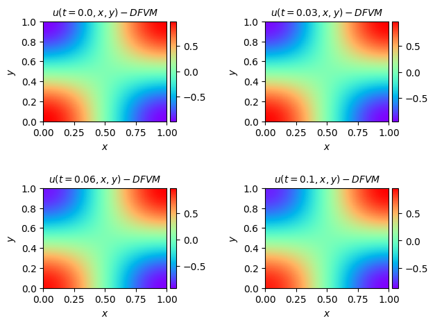
(a) DFVM solution

Fig. 3: Results of C-H equation.

3.2.3 Black-Scholes Equation

In this example, We consider the well-known Black-Scholes equation below

(39) $$\begin{cases}\displaystyle{\frac{\partial u}{\partial t}(t,x)=-\frac{1}{2}\operatorname{Tr}\left[0.16\operatorname{diag}\left(x^{2}\right)\operatorname{Hess}_{x}u(t,x)\right]+0.05(u(t,x)-(\nabla u(t,x),x)),}\\ u(T,x)=\|x\|^{2},\end{cases}$$

in $\Omega\times[0,T]$, which admits an exact solution

$$u(x,t)=\exp\left(\left(0.05+0.4^{2}\right)(T-t)\right)\|x\|^{2}.$$

The equation (39) has been discussed in [28], but here we discuss an alternative formulation of the same equation. We take $\Omega=[0,2]^{2}$ and obtain

(40) $$u_{t}=-0.08\text{div}\begin{pmatrix}\displaystyle{x_{1}^{2}\frac{\partial u}{\partial x_{1}}}\\ \displaystyle{x_{2}^{2}\frac{\partial u}{\partial x_{2}}}\end{pmatrix}+0.05u+(0.16-0.05)(\nabla u,\mathbf{x}).$$

In this test, we set $|\mathcal{T}_{r}|=1,000$, $\mathcal{T}_{b}=\{(x,T)|x\in\Omega\}$ with a size of $1,000$, and set the number of neurons of each layer to $64$.

Fig 4 illustrates the dynamic changes of the relative errors for both DFVM and PINN methods as the iteration steps and time increase. The specific numerical values are listed in Table 9, and we also evaluate the start point’s relative error of the two methods, which is defined by $\displaystyle{{\rm RE}_{0}=\frac{\|u_{\theta}(0,x)-u(0,x)\|_{L^{2}}}{\|u(0,x)\|_{L^{2}}}}$. We observe that DFVM outperforms PINN in terms of both accuracy and computational efficiency. We conclude that DFVM also performs well on parabolic PDEs.

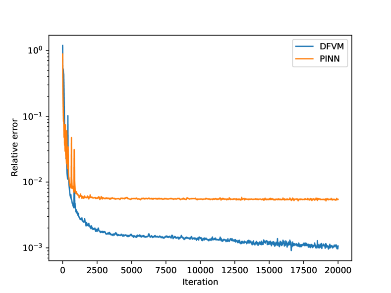
(a) RE w.r.t. iteration steps

Fig. 4: Results of Black-Scholes Equation.

Method	RE	RE0	Time (s)
DFVM	$0.10\%$	$0.16\%$	481
PINN	$0.54\%$	$0.94\%$	613

Table 9: Errors and computation time for (39).

4 Concluding remarks

We propose the DFVM, a combination of traditional method finite volume methods with deep learning methods. The key idea of the DFVM is in the loss, we calculate the second or more higher order derivatives of a network function by using a combination of first order derivatives which have been already obtained with the AD mechanism.

A deep learning method often does not suffer from the curse of dimensionality, but might suffer from the issue of low computational accuracy. The DFVM, as a paradigm combining traditional methods and deep learning methods, can ensure good computational accuracy without being plagued by the curse of dimensionality..

In this work, we present a DFVM that combine the FVM with deep learning method. The key idea in our DFVM is that we construct a FVM-based loss function. The regular n-Cube and n-Sphere are used as the control volume. The performance of DFVM is illustrated via several PDE problems including high-dimensional linear and nonlinear problems, PDEs in unbounded domains, and time-dependent PDEs. It is shown that DFVM can obtain more accurate solution with less computation cost compared with PINN, DGM and WAN.

To further improve the DFVM, we will transfer our experiences from classical numerical analysis at a deeper level. The efficient and stable DFVM for solving nonlinear time-independent equations, such as Allen-Cahn and Cahn-Hilliard equations is on the way.

References

- [1] A. G. Baydin, B. A. Pearlmutter, A. A. Radul, et al. Automatic differentiation in machine learning: a survey. Journal of Marchine Learning Research, 2018, 18: 1-43.
- [2] R. E. Caflisch. Monte Carlo and quasi-monte carlo methods. Acta numerica, 1998, 7: 1-49.
- [3] J. G. Cervera, Solution of the black-scholes equation using artificial neural networks, J. Phys. Conf. Ser. 2019,1221: 012044.
- [4] J. Chen, R. Du, P. Li and L. Lyu. Quasi-Monte Carlo Sampling for Solving Partial Differential Equations by Deep Neural Networks. Numerical Mathematics: Theory, Methods and Applications. 2021, 14(2):377-404.
- [5] X. Chen, J. Cen, Q. Zou. Adaptive trajectories sampling for solving PDEs with deep learning methods. arXiv preprint arXiv:2303.15704, 2023.
- [6] W. E, B. Yu. The Deep Ritz Method: A deep learning-based numerical algorithm for solving variational problems. Communications in mathematics and statistics, 6: 1–12 , 2018.
- [7] W. E, J. Han, A. Jentzen, Deep learning-based numerical methods for high-dimensional parabolic partial differential equations and bacc ward stochastic differential equations, Commun. Math. Stat. 2017,5 (4) :349–380.
- [8] Z. Gao, L. Yan, T. Zhou. Failure-informed adaptive sampling for PINNs. SIAM Journal on Scientific Computing, 2023, 45(4): A1971-A1994.
- [9] J. Han, L. Zhang, W. E, Solving many-electron schrödinger equation using deep neural networks, Journal of Computational Physics. 399 (2019) 108929.
- [10] K. He, X. Zhang, S. Ren, et al. Deep residual learning for image recognition. Proceedings of the IEEE conference on computer vision and pattern recognition, 770-778, 2016.
- [11] E. Kharazmi, Z. Zhang, G. Karniadakis. hp-VPINNs: Variational physics-informed neural networks with domain decomposition. Computer Methods in Applied Mechanics and Engineering, 2021, 374:113547.
- [12] Liao, Yulei, and Pingbing Ming. ”Deep nitsche method: Deep ritz method with essential boundary conditions.” arXiv preprint arXiv:1912.01309 (2019).
- [13] Sheng, Hailong, and Chao Yang. ”PFNN: A penalty-free neural network method for solving a class of second-order boundary-value problems on complex geometries.” Journal of Computational Physics 428 (2021): 110085.
- [14] D. P. Kingma, J. L. Ba. Adam: A Method for Stochastic Optimization, arXiv:1412.6980, 2014.
- [15] P. K. Kundu, I. M. Cohen, D. R. Dowling. Fluid mechanics. Academic press, 2015.
- [16] H. Kurt, Approximation capabilities of multilayer feedforward networks, Neural Networks. 4 (2), 251–257, 1991.
- [17] H. Kurt; T. Maxwell, W. Halbert, Multilayer feedforward networks are universal approximators (PDF). Neural Networks, 2, 359–366, 1989.
- [18] Y. LeCun, Y. Bengio, G. Hinton. Deep learning. nature, 2015, 521(7553): 436-444.
- [19] R. LeVeque. Finite Difference Methods for Ordinary and Partial Differential Equations: Steady-State and Time-Dependent Problems. SIAM, 2007.
- [20] Z. Li, N. Kovachki, K. Azizzadenesheli, et al. Fourier neural operator for parametric partial differential equations. arXiv preprint arXiv:2010.08895, 2020.
- [21] L. Lu, P. Jin, G. Pang, et al. Learning nonlinear operators via deeponet based on the universal approximation theorem of operators. Nature Machine Intelligence, 2021,3(3):218–229.
- [22] L. Lu, X. Meng, Z. Mao, et al. DeepXDE: A deep learning library for solving differential equations, SIAM Rev. 2021,63(1): 208–228.
- [23] L. Lyu, Z. Zhang, J. Chen, et al. MIM: A deep mixed residual method for solving high order partial differential equations. Journal of Computational Physics, 2022, 452(1): 110930.
- [24] C. C. Margossian. A review of automatic differentiation and its efficient implementation. Wiley interdisciplinary reviews: data mining and knowledge discovery, 2019, 9(4): e1305.
- [25] M. Nabian, R.Gladstone, H. Meidani, Efficient training of physics-informed neural networks via importance sampling, Computer-Aided Civil and Infrastructure Engineering,2021,36(8):597-1090.
- [26] W. F. Pfeffer. The divergence theorem. Transactions of the American Mathematical Society 295.2 (1986): 665-685.
- [27] A. Pinkus. Approximation theory of the MLP model in neural networks. Acta numerica, 1999, 8: 143-195.
- [28] M. Raissi. Forward-backward stochastic neural networks: Deep learning of high-dimensional partial differential equations, arXiv: 1804.07010, 2018.
- [29] Han, Jihun, Mihai Nica, and Adam R. Stinchcombe. ”A derivative-free method for solving elliptic partial differential equations with deep neural networks.” Journal of Computational Physics 419 (2020): 109672.
- [30] M. Raissi, P. Perdikaris and G.E. Karniadakis. Physics-informed neural networks: A deep learning framework for solving forward and inverse problems involving nonlinear partial differential equations, Journal of Computational Physic, 378, 686-707,2019.
- [31] Berg, Jens, and Kaj Nyström. ”A unified deep artificial neural network approach to partial differential equations in complex geometries.” Neurocomputing 317 (2018): 28-41.
- [32] D. E. Rumelhart, G. E. Hinton, R.J. Williams. Learning representations by back-propagating errors. nature, 1986, 323(6088): 533-536.
- [33] M. V. Shcherbakov, A. Brebels, N. L. Shcherbakova, A. P. Tyukov, T. A. Janovsky, V. A. E. Kamaev. A survey of forecast error measures. World applied sciences journal. 2013, 24(24), 171-176.
- [34] J. Sirignano, K. Spiliopoulosb. DGM: A deep learning algorithm for solving partial differential equations, Journal of Computational Physics, 375:1339-1364, 2018.
- [35] I. Smears, E. Suli. Discontinuous Galerkin finite element approximation of nondivergence form elliptic equations with Cordes coefficients. SIAM Journal on Numerical Analysis, 2013, 51(4): 2088-2106.
- [36] K. Tang, X. Wan, C. Yang. DAS-PINNs: A deep adaptive sampling method for solving high-dimensional partial differential equations. Journal of Computational Physics, 2023, 476: 111868.
- [37] J. Xu, Q. Zou, Analysis of linear and quadratic finite volume methods for elliptic equations, Numer. Math., 2009, 111: 469-492.
- [38] Y. Zang, G. Bao, X. Ye, H. Zhou, Weak adversarial networks for high-dimensional partial differential equations, Journal of Computational Physic, 411: 109409, 2020.
- [39] S. Zeng, Z. Zhang, Q. Zou. Adaptive deep neural networks methods for high-dimensional partial differential equations. Journal of Computational Physics, 2022, 463: 111232.
- [40] D. Zhang, L. Lu, L. Guo, et al., Quantifying total uncertainty in physics-informed neural networks for solving forward and inverse stochastic problems, Journal of Computational Physics, 2019,397: 108850.
- [41] Y. Zhu, N. Zabaras, P. Koutsourelakiset et al., Physics-constrained deep learning for high-dimensional surrogate modeling and uncertainty quantification without labeled data, Journal of Computational Physics, 2019,394: 56–81.
- [42] O. Zienkiewicz, R. Taylor, and J. Zhu. The Finite Element Method: Its Basis and Fundamentals. Elsevier, 2005.