Enhancing Datalog Reasoning with Hypertree Decompositions

Abstract

Datalog reasoning based on the seminaïve evaluation strategy evaluates rules using traditional join plans, which often leads to redundancy and inefficiency in practice, especially when the rules are complex. Hypertree decompositions help identify efficient query plans and reduce similar redundancy in query answering. However, it is unclear how this can be applied to materialisation and incremental reasoning with recursive Datalog programs. Moreover, hypertree decompositions require additional data structures and thus introduce nonnegligible overhead in both runtime and memory consumption. In this paper, we provide algorithms that exploit hypertree decompositions for the materialisation and incremental evaluation of Datalog programs. Furthermore, we combine this approach with standard Datalog reasoning algorithms in a modular fashion so that the overhead caused by the decompositions is reduced. Our empirical evaluation shows that, when the program contains complex rules, the combined approach is usually significantly faster than the baseline approach, sometimes by orders of magnitude.

1 Introduction

Datalog (Abiteboul et al., 1995) is a widely used rule language that can express recursive dependencies, such as graph reachability and transitive closure. Reasoning in Datalog has found applications in different areas and supports a wide range of tasks including consistency checking (Luteberget et al., 2016) and data analysis (Alvaro et al., 2010). Datalog is also able to capture OWL 2 RL ontologies (Motik et al., 2009) extended with SWRL rules (Horrocks et al., 2004) and can thus support query answering over ontology-enriched data; it has been implemented in a growing number of open-source and commercial systems, such as VLog (Carral et al., 2019), LogicBlox (Aref et al., 2015), Vadalog (Bellomarini et al., 2018), RDFox (Nenov et al., 2015), Oracle’s database (Wu et al., 2008), and GraphDB.

In a typical application, Datalog is used to declaratively represent domain knowledge as ‘if-then’ rules. Given a set of explicit facts and a set of rules, Datalog systems are required to answer queries over all the facts entailed by the given rules and facts. To facilitate query answering, the entailed facts are often precomputed in a preprocessing step; we use materialisation to refer to both this process and the resulting set of facts. Queries can then be evaluated directly over the materialisation without considering the rules. The materialisation can be efficiently computed using the seminaïve algorithm (Abiteboul et al., 1995), which ensures that each inference is performed only once. Incremental maintenance algorithms can then be used to avoid the cost of recomputing the materialisation when explicitly given facts are added/deleted; these include general algorithms such as the counting algorithm (Gupta et al., 1993), the Delete/Rederive (DRed) algorithm (Staudt and Jarke, 1995), and the Backward/Forward (B/F) algorithm (Motik et al., 2015), as well as special purpose algorithms designed for rules with particular shapes (Subercaze et al., 2016). It has recently been shown that general and special purpose algorithms can be combined in a modular framework that supports both materialisation and incremental maintenance (Hu et al., 2022).

Existing (incremental) materialisation algorithms implicitly assume that the evaluation of rule bodies is based on traditional join plans which can be suboptimal in many cases (Ngo et al., 2014; Gottlob et al., 2016), especially in the case of cyclic rules. This can lead to a blow-up in the number of intermediate results and a corresponding degradation in performance (as we demonstrate in Section 5). This phenomenon can be observed in real-life applications, for example where rules are used to model complex systems, which may include the evaluation of numerical expressions. The resulting rules are often cyclic and have large numbers of body atoms.

Similar problems also exist in query answering. One promising solution is based on hypertree decomposition (Gottlob et al., 2016). Hypertree decomposition is able to decompose cyclic queries, and Yannakakis’s algorithm (Yannakakis, 1981) can then be used to achieve efficient evaluation over the decomposition (Gottlob et al., 2016). This method has been well-investigated with its effectiveness shown in many empirical experiments for query evaluation (Tu and Ré, 2015; Aberger et al., 2016).

It is unclear, however, whether the hypertree decomposition approach can benefit rule evaluation in Datalog reasoning. Unlike query answering, which requires only a single evaluation via decomposition, rules in a Datalog program are applied multiple times until no new data can be derived. In this setting, it is important to avoid repetitive derivations, but this is not easy to achieve when hypertree decomposition is used for rule evaluation. Moreover, incremental materialisation usually depends on efficiently tracking fact derivations, and it is unclear how to achieve this when such derivations depend on hypertree decomposition. Finally, hypertree decomposition introduces some additional overhead, and this may degrade performance on simple rules.

In this paper, we introduce a Datalog reasoning algorithm that exploits hypertree decomposition to provide efficient (incremental) reasoning of recursive programs. Moreover, we show how this algorithm can be combined with the seminaïve algorithm in a modular framework so as to avoid unnecessary additional overhead on simple rules. Our empirical evaluation shows that this combined approach significantly outperforms the standard approach, sometimes by orders of magnitude, and it is never significantly slower. Our test system and data are available online. Proofs and additional evaluation results are included in a technical report (Zhang et al., 2023).

2 Preliminaries

Datalog: A term is a variable or a constant. An atom is an expression of the form $P(t_{1},...,t_{k})$ where $P$ is a predicate with arity $k$, $k\geq 0$, and each $t_{i}$, $1\leq i\leq k$, is a term. A fact is a variable-free atom, and a dataset is a finite set of facts. A rule is an expression of the following form:

$$B_{0}\wedge\dots\wedge B_{n}\rightarrow H,$$ (1)

where $n\geq 0$ and $B_{i}$, $0\leq i\leq n$, and $H$ are atoms. For $r$ a rule, $\mathsf{h}(r)=H$ is its head, and $\mathsf{b}(r)=\{B_{0},\dots,B_{n}\}$ is the set of body atoms. For $S$ an atom or a set of atoms, $\mathsf{var}(S)$ is the set of variables appearing in $S$. For a rule $r$ to be safe, each variable occurring in its head must also occur in at least one of its body atoms, i.e., $\mathsf{var(h}(r))\subseteq\mathsf{var(b}(r))$. A program is a finite set of safe rules.

A substitution $\sigma$ is a mapping of finitely many variables to constants. For $\alpha$ a term, an atom, a rule, or a set of them, $\alpha\sigma$ is the result of replacing each occurrence of a variable $x$ in $\alpha$ with $\sigma(x)$ if $\sigma(x)$ is defined in $\sigma$. For a rule $r$ and a substitution $\sigma$, if $\sigma$ maps all the variables occurring in $r$ to constants, then $r\sigma$ is an instance of $r$.

For a rule $r$ and a dataset $I$, $r[I]$ is the set of facts obtained by applying $r$ to $I$:

$$r[I]=\{\mathsf{h}(r\sigma)\ |\ \mathsf{b}(r\sigma)\subseteq I\}.$$ (2)

Moreover, for a program $\Pi$ and a dataset $I$, $\Pi[I]$ is the set obtained by applying every rule $r$ in $\Pi$ to $I$:

$$\Pi[I]=\bigcup_{r\in\Pi}\{r[I]\}.$$ (3)

For E a dataset, let $I_{0}=E$, and we define the materialisation $I_{\infty}$ of $\Pi$ w.r.t. $E$ as:

$$I_{\infty}=\bigcup_{i\geq 0}I_{i},\text{ where }I_{i}=I_{i-1}\cup\Pi[I_{i-1}]\text{ for }i>0.$$ (4)

Seminaïve Algorithm: We will briefly introduce the seminaïve algorithm to facilitate our discussion in later sections. As we shall see, our algorithms exploit similar techniques to avoid repetition in reasoning.

Algorithm 1 MAT($\Pi,E$)

1:$I\leftarrow\emptyset$

2:$\Delta\leftarrow E$

3:while $\Delta\neq\emptyset$ do

4:     $I:=I\cup\Delta$

5:     $\Delta:=\Pi[I\,\begin{subarray}{c}\cdot\\[-3.41418pt] \cdot\\[-3.41418pt] \cdot\\[1.42271pt] \end{subarray}\,\Delta]\ \backslash\ I$

The seminaïve algorithm (Abiteboul et al., 1995) realises non-repetitive reasoning by identifying newly derived facts in each round of rule application. Given a program $\Pi$ and a set of facts $E$, the algorithm computes the materialisation $I$ of $\Pi$ w.r.t. $E$. As shown in Algorithm 1, $\Delta$ is initialised as $E$. In each round of rule applications, the algorithm will first update $I$ by adding to it the newly derived facts from the previous round and then computing a fresh set of derived facts using the operator $\Pi$ defined as below:

$$r[I\,\begin{subarray}{c}\cdot\\[-3.41418pt] \cdot\\[-3.41418pt] \cdot\\[1.42271pt] \end{subarray}\,\Delta]=\{\mathsf{h}(r\sigma)\ |\ \mathsf{b}(r\sigma)\subseteq I\ \text{and}\ \mathsf{b}(r\sigma)\cap\Delta\neq\emptyset\},$$ (5)

$$\Pi[I\,\begin{subarray}{c}\cdot\\[-3.41418pt] \cdot\\[-3.41418pt] \cdot\\[1.42271pt] \end{subarray}\,\Delta]=\bigcup_{r\in\Pi}\{r[I\,\begin{subarray}{c}\cdot\\[-3.41418pt] \cdot\\[-3.41418pt] \cdot\\[1.42271pt] \end{subarray}\,\Delta]\},$$ (6)

in which $\sigma$ in expression (5) is a substitution mapping variables in $r$ to constants, and $\Delta\subseteq I$. The definition of $\Pi[I\,\begin{subarray}{c}\cdot\\[-3.41418pt] \cdot\\[-3.41418pt] \cdot\\[1.42271pt] \end{subarray}\,\Delta]$ ensures that the algorithm will only consider rule instances that have not been considered before. In practice, $r[I\,\begin{subarray}{c}\cdot\\[-3.41418pt] \cdot\\[-3.41418pt] \cdot\\[1.42271pt] \end{subarray}\,\Delta]$ can be efficiently implemented by evaluating the rule body $n+1$ times (Motik et al., 2019). Specifically, for the $i$th evaluation, $0\leq i\leq n$, the body is evaluated by:

$$B_{0}^{I\backslash\Delta}\wedge\dots\wedge B_{i-1}^{I\backslash\Delta}\wedge B_{i}^{\Delta}\wedge B_{i+1}^{I}\wedge\dots\wedge B_{n}^{I},$$ (7)

in which the superscript identifies the set of facts where each atom is matched.

DRed Algorithm: The original DRed algorithm is presented by Gupta et al. (1993), but it does not support non-repetitive reasoning. In this paper, we consider a non-repetitive and generalised version of the DRed algorithm presented by Hu et al. (2022). This version of the DRed algorithm allows modular reasoning, i.e., reasoning over different parts of the program can be implemented using customised algorithms, which is more suitable for our discussions below.

The DRed algorithm is shown in Algorithm 2 where input arguments $\Pi$ and $E$ represent the program and the original set of explicitly given facts, $I$ is the materialisation of $\Pi$ w.r.t. $E$, and $E^{+}$ and $E^{-}$ are the sets of facts that are to be added to and deleted from $E$, respectively. As shown in lines 2–4, the main idea behind DRed is to first overdelete all possible derivations that depend on $E^{-}$; and then the algorithm tries to rederive facts that have alternative proofs using the remaining facts; lastly, to add to the materialisation, the algorithm computes the consequences of $E^{+}$ as well as the rederived facts.

Specifically, overdeletion involves recursively finding all the consequences derived by $\Pi$ and $E^{-}$, directly or indirectly, as shown in lines 7–14. The function $\mathsf{Del}^{r}$ called in line 13 is intended to compute the facts that are directly affected by the deletion of $\Delta^{-}$. More precisely, $\mathsf{Del}^{r}(I,\Delta^{-})$ should compute ${r[I\,\begin{subarray}{c}\cdot\\[-3.41418pt] \cdot\\[-3.41418pt] \cdot\\[1.42271pt] \end{subarray}\,\Delta^{-}]}\cap(I\backslash\Delta^{-})$. Note that in line 13 the first argument of the call is $I\backslash D$, so it should compute ${r[I^{\prime}\,\begin{subarray}{c}\cdot\\[-3.41418pt] \cdot\\[-3.41418pt] \cdot\\[1.42271pt] \end{subarray}\,\Delta^{-}]}\cap(I^{\prime}\backslash\Delta^{-})$ with ${I^{\prime}=I\backslash D}$; the same clarification applies to $\mathsf{Red}^{r}$ and $\mathsf{Add}^{r}$, so we will not reiterate.

The rederivation step recovers the facts that are overdeleted but are one-step provable from the remaining facts. Formally, function $\mathsf{Red}^{r}(I,\Delta)$ should compute ${r[I]\cap\Delta}$. Finally, during addition, the added set $N_{A}$ is initialised in line 21, and then from line 22 to 28 the rules are iteratively applied, similarly as in the seminaïve algorithm. In this case, function $\mathsf{Add}^{r}(I,\Delta^{+})$ is required to compute ${r[I\,\begin{subarray}{c}\cdot\\[-3.41418pt] \cdot\\[-3.41418pt] \cdot\\[1.42271pt] \end{subarray}\,\Delta^{+}]}\backslash I$.

The correctness of Algorithm 2 is guaranteed by Theorem 1, which straightforwardly follows from the correctness of the modular update algorithm by Hu et al. (2022).

Theorem 1.

Algorithm 2 correctly updates the materialisation $I_{\infty}$ of $\Pi$ w.r.t. $E$ to $I^{\prime}_{\infty}$ of $\Pi$ w.r.t. $E^{\prime}$ where $E^{\prime}=(E\backslash E^{-})\cup E^{+}$, provided that $\mathsf{Del}^{r}(I,\Delta^{-})$, $\mathsf{Red}^{r}(I,\Delta)$, and $\mathsf{Add}^{r}(I,\Delta^{+})$ compute ${r[I\,\begin{subarray}{c}\cdot\\[-3.41418pt] \cdot\\[-3.41418pt] \cdot\\[1.42271pt] \end{subarray}\,\Delta^{-}]\cap(I\backslash\Delta^{-})}$, ${r[I]\cap\Delta}$, and ${r[I\,\begin{subarray}{c}\cdot\\[-3.41418pt] \cdot\\[-3.41418pt] \cdot\\[1.42271pt] \end{subarray}\,\Delta^{+}]\backslash I}$, respectively.

Please note that the DRed algorithm could be used for the initial materialisation as well. To achieve this, we can set $E,\ I$ and $E^{-}$ as empty sets, and pass the set of explicitly given facts as $E^{+}$ to the algorithm.

Algorithm 2 DRed($\Pi,E,I,E^{+},E^{-}$)

1:$D:=A:=\emptyset$, $E^{-}:=(E^{-}\cap E)\backslash E^{+}$, $E^{+}:=E^{+}\backslash E$

2:Overdelete

3:Rederive

4:Add

5:$E:=(E\backslash E^{-})\cup E^{+}$, $I:=(I\backslash D)\cup A$

6:procedure Overdelete

7:     $N_{D}:=E^{-}$

8:     loop

9:         $\Delta^{-}:=N_{D}\backslash D$

10:         if $\Delta^{-}=\emptyset$ then break          

11:         $N_{D}:=\emptyset$

12:         for $r\in\Pi$ do

13:              $N_{D}:=N_{D}\cup\mathsf{Del}^{r}(I\backslash D,\Delta^{-})$          

14:         $D:=D\cup\Delta^{-}$      

15:procedure Rederive

16:     $\Delta:=\emptyset$

17:     for $r\in\Pi$ do

18:         $\Delta:=\Delta\cup\mathsf{Red}^{r}(I\backslash D,D)$      

19:     $\Delta:=\Delta\cup((E\backslash E^{-})\cap D)$

20:procedure Add

21:     $N_{A}:=(\Delta\cup E^{+})\backslash(I\backslash D)$

22:     loop

23:         $\Delta^{+}:=N_{A}\backslash((I\backslash D)\cup A)$

24:         if $\Delta^{+}=\emptyset$ then break          

25:         $A:=A\cup\Delta^{+}$

26:         $N_{A}:=\emptyset$

27:         for $r\in\Pi$ do

28:              $N_{A}:=N_{A}\cup\mathsf{Add}^{r}((I\backslash D)\cup A,\Delta^{+})$               

Hypertree Decomposition: Following the definition of hypertree decomposition for conjunctive queries (Gottlob et al., 2002), we define it for Datalog rules in a similar way.

For a Datalog rule $r$, a hypertree decomposition is a hypertree $HD=\langle T,\chi,\lambda\rangle$ in which $T=\langle N,E\rangle$ is a rooted tree, and $\chi$ associates each vertex $p\in N$ with a set of variables in $r$ whereas $\lambda$ associates $p$ with a set of atoms in $\mathsf{b}(r)$. This hypertree satisfies all the following conditions:

1. for each body atom $B_{i}\in\mathsf{b}(r)$, there exists $p\in N$ such that $\mathsf{var}(B_{i})\subseteq\chi(p);$

2. for each variable $v\in\mathsf{var}(r)$, the set $\{p\in N\ |\ v\in\chi(p)\}$ induces a connected subtree of $T$.

3. for each vertex $p\in N$, $\chi(p)\subseteq\mathsf{var}(\lambda(p))$.

4. for each vertex $p\in N$, $\mathsf{var}(\lambda(p))\cap\chi(T_{p})\subseteq\chi(p)$ in which $T_{p}$ is the subtree of T rooted at $p$.

The width of the hypertree decomposition is defined as $max_{p\in N}|\lambda(p)|$. The hypertree-width hw(r) of $r$ is the minimum width over all possible hypertree decompositions of $r$. In this paper, we refer to $r$ as a complex rule, or interchangeably, a cyclic rule, if and only if its hypertree width $hw(r)$ is greater than 1.

Next, we will introduce how query evaluation works using a decomposition as join plan. Query evaluation via hypertree decomposition is a well-investigated problem in the database literature (Gottlob et al., 2016; Flum et al., 2002), and such a process typically consists of in-node evaluation and cross-node evaluation. During in-node evaluation, each node $p$ in the decomposition joins the body atoms that are assigned to it (i.e., $\lambda(p)$) and stores the join results for later use. Then, cross-node evaluation applies the Yannakakis algorithm to the above join results using $T$ as the join tree. The standard Yannakakis algorithm in turn has two steps. The full reducer stage applies a sequence of bottom-up left semi-joins through the tree, followed by a sequence of top-down left semi-joins using the same fixed root of the tree (Bernstein and Chiu, 1981). This removes dangling data that will not be needed in the second stage and decreases the join result size for each node. The cross-node join stage joins the nodes bottom-up, and it projects to the output variables, i.e., $\mathsf{var}(\mathsf{h}(r))$, to obtain the final answers.

Overall, the (combined) complexity of query evaluation via a decomposition tree is known to be $O(v\cdot(m^{k}+s)\cdot log(m+s))$ (Gottlob et al., 2016) where $v$ is the number of variables in the query, $m$ is the cardinality of the largest relation in data, $k$ is the hypertree width of $r$, and $s$ is the output size.

3 Motivation

In this section, we use an example to explain how hypertree decompositions could benefit rule evaluation and provide some intuitions as to how they can be exploited in the evaluation of recursive Datalog rules. To this end, consider the following rule $r$, in which $\mathsf{PC,CW}$ and $\mathsf{CA}$ represent $\mathsf{PossibleCollaborator}$, $\mathsf{Coworker}$, and $\mathsf{Coauthor}$, respectively:

$$\mathsf{PC}(x,y)\leftarrow\mathsf{CW}(x,z_{1}),\mathsf{CA}(x,z_{2}),\mathsf{PC}(z_{1},y),\mathsf{PC}(z_{2},y).$$

Moreover, consider the dataset $E$ as specified below, where $n$ and $k$ are constants. Refer to Figure 1 for a (partial) illustration of the dataset and the joins.

$$\{\mathsf{CW}(a_{i},b_{i\cdot k+j})\mid 0\leq i<n,\quad 1\leq j\leq k\}\;\cup$$

$$\{\mathsf{CA}(a_{i},c_{i\cdot k+j})\mid 0\leq i<n,\quad 1\leq j\leq k\}\;\cup$$

$$\{\mathsf{CW}(a_{n},a_{2}),\quad\mathsf{CA}(a_{n},a_{3})\}\;\cup$$

$$\{\mathsf{PC}(b_{i\cdot k+j},d_{j})\mid 0\leq i<n,\quad 1\leq j\leq k\}\;\cup$$

$$\{\mathsf{PC}(c_{i\cdot k+j},d_{j})\mid 0\leq i<n,\quad 1\leq j\leq k\}$$

Each relation above contains $O(n\cdot k)$ facts, and the materialisation will additionally derive ${n\cdot k+k}$ facts, i.e., $\{\mathsf{PC}(a_{i},d_{j})\mid 0\leq i\leq n,\quad 1\leq j\leq k\}$.

Now consider the first round of rule evaluation, and assume that the rule body of $r$, which corresponds to a conjunctive query, is evaluated left-to-right. Then, matching the first three atoms involves considering $O(n\cdot k^{2})$ different substitutions for variables $x$, $y$, $z_{1}$, and $z_{2}$; only $O(n\cdot k)$ of them will match the last atom and eventually lead to successful derivations. In fact, one can verify that no matter how we reorder the body atoms of $r$, it will result in similar behaviour.

Using hypertree decompositions could help process the query more efficiently. Consider decomposition $T$ of the above query consisting of two nodes $p_{1}$ and $p_{2}$, where $p_{1}$ is the parent node of $p_{2}$. Furthermore, function $\chi$ is defined as: $\chi(p_{1})=\{x,z_{1},y\}$, $\chi(p_{2})=\{x,z_{2},y\}$, and function $\lambda$ is defined as: $\lambda(p_{1})=\{\mathsf{CW}(x,z_{1}),\mathsf{PC}(z_{1},y)\}$, $\lambda(p_{2})=\{\mathsf{CA}(x,z_{2}),\mathsf{PC}(z_{2},y)\}$. Recall the steps of decomposition-based query evaluation we introduced in Section 2. During the in-node evaluation stage, each node in the decomposition will consider $O(n\cdot k)$ substitutions; the full reducer will consider $O(n\cdot k)$ substitutions and find out that nothing needs to be reduced; lastly, the cross-node evaluation joining $p_{1}$ and $p_{2}$ also considers $O(n\cdot k)$ substitutions. Compared with the left-to-right evaluation of the query, the overall cost of this approach is $O(n\cdot k)$, as opposed to $O(n\cdot k^{2})$. For every $a_{i}$ ($0\leq i<n$), the first round of rule application will introduce additional $\mathsf{PC}$ relations between $a_{i}$ and $d_{1}$ to $d_{k}$ ($n\cdot k$ in total).

Notice that rule $r$ is recursive, so the facts produced by the first round of rule evaluation could potentially lead to further derivations of the same rule. This is indeed the case in our example: the first round derives all $\mathsf{PC}(a_{i},d_{j})$ facts with ${0\leq i<n}$ and ${1\leq j\leq k}$; combined with $\{\mathsf{CW}(a_{n},a_{2}),\mathsf{CA}(a_{n},a_{3})\}$ this will additionally derive ${\mathsf{PC}(a_{n},d_{j})}$ with ${1\leq j\leq k}$. If we used the hypertree decomposition-based technique discussed above, then a naïve implementation would just add all the facts derived in the first round to the corresponding nodes and run the decomposition-based query evaluation again. However, this is unlikely to be very efficient as it would have to repeat all the work performed in the first round of rule evaluation. Ideally, we would like to make the decomposition-based query evaluation algorithm ‘incremental’, in the sense that the algorithm minimises the amount of repeated work between different rounds of rule evaluation. As we shall see in Section 4, this requires nontrivial adaptation of in-node evaluation, as well as the two stages of the Yannakakis algorithm. Handling incremental deletion presents another challenge, which we address following the well-known DRed algorithm.

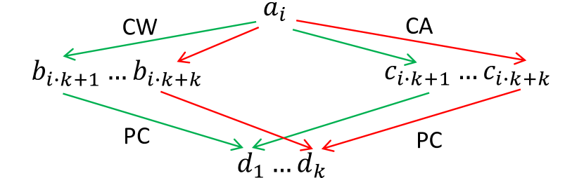
Figure 1: Illustration of joins related to a particular $a_{i}$, $0\leq i<n$, in the first round of rule evaluation.

4 Algorithms

We now introduce our reasoning algorithms based on hypertree decomposition. We use DRed as the backbone of our algorithm, but instead of standard reasoning algorithms with plan-based rule evaluation, we will use our hypertree decomposition-based functions $\mathsf{Del}^{r}$, $\mathsf{Add}^{r}$, and $\mathsf{Red}^{r}$ as discussed below. For each rule $r$ in $\Pi$, we assume its hypertree decomposition $\langle T^{r},\chi^{r},\lambda^{r}\rangle$ with ${T^{r}=\langle N^{r},E^{r}\rangle}$ has already been computed, and $t^{r}$ is the root of the decomposition tree $T^{r}$. Our reasoning algorithms are independent of decomposition methods.

Notation: First, analogously to expression (5), for each node $p\in N^{r}$ we define operator $\Pi_{p}[I,\Delta]$, in which $I$ and $\Delta$ are sets of facts with $\Delta\subseteq I$.

$$\Pi_{p}[I,\Delta]=\{\chi^{r}(p)\sigma\ |\ \lambda^{r}(p)\sigma\subseteq I\text{ and }\\ \lambda^{r}(p)\sigma\cap\Delta\nsubseteq\emptyset\},$$

Intuitively, this operator is intended to compute for a node $p$ all the instantiations influenced by the incremental update $\Delta$. Additionally, for each node $p\in N^{r}$, we will make use of the following sets in the presentation of our algorithms. These sets are initialised as empty the first time DRed is executed.

1. $\mathsf{inst}_{p}^{I}$ contains the join result of in-node evaluation for $p$ under the current materialisation $I$, and it is represented as tuples for variables $\chi^{r}(p)$. Since cross-node evaluation builds upon such join results, to facilitate incremental evaluation and to avoid computing $\mathsf{inst}_{p}^{I}$ every time from scratch, $\mathsf{inst}_{p}^{I}$ has to be correctly maintained between different executions of DRed.

2. $\mathsf{inst}_{p}^{I\,\begin{subarray}{c}\cdot\\[-3.41418pt] \cdot\\[-3.41418pt] \cdot\\[1.42271pt] \end{subarray}\,\Delta^{+}}$ represents the set of instantiations that should be added to $\mathsf{inst}_{p}^{I}$ given a set of newly added facts $\Delta^{+}$. This set can be obtained using the operator $\Pi_{p}$.

3. $\mathsf{inst}_{p}^{I\,\begin{subarray}{c}\cdot\\[-3.41418pt] \cdot\\[-3.41418pt] \cdot\\[1.42271pt] \end{subarray}\,\Delta^{-}}$ represents the set of instantiations that no longer hold after removing $\Delta^{-}$ from $I$; these instantiations should then be deleted from $\mathsf{inst}_{p}^{I}$. Similarly as above, this set can be computed using $\Pi_{p}$.

4. $\mathsf{inst}_{p}^{ac}$ represents the currently active instantiations that will participate in the cross-node evaluation.

5. $\mathsf{inst}_{p}^{re}$ represents the instantiations that will need to be checked during the rederivation phase.

Algorithm 3 $\mathsf{Add}^{r}[I,\Delta^{+}]$

1:/* in-node evaluation */

2:for $p\in N^{r}$ do:

3:     $\mathsf{inst}_{p}^{I\,\begin{subarray}{c}\cdot\\[-3.41418pt] \cdot\\[-3.41418pt] \cdot\\[1.42271pt] \end{subarray}\,\Delta^{+}}:=\Pi_{p}[I,\Delta^{+}]\ \backslash\ \mathsf{inst}_{p}^{I}$

4:/* cross-node evaluation */

5:$\Delta_{A}:=\mathsf{CrossNodeEvaluation}^{r}(\mathsf{L^{+}})$

6:/* updating instantiations for each node */

7:for $p\in N^{r}$ do

8:     $\mathsf{inst}_{p}^{I}:=\mathsf{inst}_{p}^{I}\cup\mathsf{inst}_{p}^{I\,\begin{subarray}{c}\cdot\\[-3.41418pt] \cdot\\[-3.41418pt] \cdot\\[1.42271pt] \end{subarray}\,\Delta^{+}}$

9:     $\mathsf{inst}_{p}^{I\,\begin{subarray}{c}\cdot\\[-3.41418pt] \cdot\\[-3.41418pt] \cdot\\[1.42271pt] \end{subarray}\,\Delta^{+}}:=\emptyset$

10:return $\Delta_{A}\backslash I$

Addition: As discussed in Section 3, the decomposition-based query evaluation should be made incremental. To this end, Algorithm 3, which is responsible for addition, needs to distinguish between old instantiations and the new ones added due to changes in the explicitly given data. This is achieved by executing the in-node evaluation for each node $p\in N^{r}$ in line 3 using the $\Pi_{p}$ operator. Then, the cross-node evaluation (line 5) is performed in a way similar to the evaluation of $r[I\,\begin{subarray}{c}\cdot\\[-3.41418pt] \cdot\\[-3.41418pt] \cdot\\[1.42271pt] \end{subarray}\,\Delta]$ outlined in Section 2, treating each node in $T^{r}$ as a body atom. Specifically, as shown in algorithm 4, we will evaluate the tree $|N^{r}|$ times. Assume that there is a fixed order among all the tree nodes for $r$, and let $p_{i}$, $1\leq i\leq|N^{r}|$, denote the $i$th node in this ordering. Then, in the $i$th iteration of the loop of lines 2–8, node $p_{i}$ is chosen in line 2, and the label of each node will be determined by the labelling function $\mathsf{L}^{+}$ as specified below. In particular, node $p_{i}$ will be labelled $\Delta^{+}$; nodes preceding and succeeding $p_{i}$ will be labelled $I$ and $I\cup\Delta^{+}$, respectively.

$$\mathsf{L^{+}}(p_{i},p_{j})=\left\{\begin{array}[]{lr}I\cup\Delta^{+},&p_{j}\prec p_{i}\\ \Delta^{+},&p_{j}=p_{i}\\ I,&p_{j}\succ p_{i}\end{array}.\right.$$ (8)

Based on the labels assigned in line 4, we will set $p_{j}^{ac}$, the active instantiations that will participate in the subsequent evaluation, as follows. Note that the last two cases will be used later for deletion.

$$\mathsf{inst}_{p}^{ac}=\left\{\begin{array}[]{ll}\mathsf{inst}_{p}^{I}&I\\ \mathsf{inst}_{p}^{I\,\begin{subarray}{c}\cdot\\[-3.41418pt] \cdot\\[-3.41418pt] \cdot\\[1.42271pt] \end{subarray}\,\Delta^{+}}&\Delta^{+}\\ \mathsf{inst}_{p}^{I}\cup\mathsf{inst}_{p}^{I\,\begin{subarray}{c}\cdot\\[-3.41418pt] \cdot\\[-3.41418pt] \cdot\\[1.42271pt] \end{subarray}\,\Delta^{+}}&I\cup\Delta^{+}\\ \mathsf{inst}_{p}^{I\,\begin{subarray}{c}\cdot\\[-3.41418pt] \cdot\\[-3.41418pt] \cdot\\[1.42271pt] \end{subarray}\,\Delta^{-}}&\Delta^{-}\\ \mathsf{inst}_{p}^{I}\backslash\mathsf{inst}_{p}^{I\,\begin{subarray}{c}\cdot\\[-3.41418pt] \cdot\\[-3.41418pt] \cdot\\[1.42271pt] \end{subarray}\,\Delta^{-}}&I\backslash\Delta^{-}\end{array}.\right.$$ (9)

After fixing the active instantiations, algorithm 4 proceeds with an adapted version of the Yannakakis algorithm: lines 6–7 complete the full reducer stage whereas line 8 performs the cross-node join. By performing left semi-joins between nodes, the full reducer stage aims at deactivating instantiations that do not join and keep only the relevant ones. The standard full reducer does not consider incremental updates so adaptations are required. In particular, our incremental version of the full reducer traverses the tree three times. The first traversal in line 6 consists of a sequence of top-down left semi-joins with $p_{i}$ (the node labelled with $\Delta^{+}$) as the root. As $\Delta^{+}$ is typically smaller than the materialisation $I$, starting from $p_{i}$ could potentially reduce the numbers of active instantiations for the other nodes to a large extent. The second and the third traversal (line 7) involves applying the standard bottom-up and top-down left semi-join sequences, respectively, using the root of the decomposition tree $t^{r}$ as the root for the evaluation. Then, the cross-node join in line 8 evaluates the decomposition tree $T^{r}$ bottom-up: for each node $p\in N^{r}$, it joins active instantiations in $p$ with those in its children, and then projects the result to variables $\chi^{r}(p)\ \cup\ \mathsf{var(h}(r))$. The join result obtained at the root $t^{r}$ is projected to the output variables $\mathsf{var(h}(r))$ to compute the derived facts, which are then returned to the $\mathsf{Add}^{r}$ function.

Lastly, lines 7–9 of algorithm 3 update the instantiations $\mathsf{inst}_{p}^{I}$ for each node $p$ and empty $\mathsf{inst}_{p}^{I\,\begin{subarray}{c}\cdot\\[-3.41418pt] \cdot\\[-3.41418pt] \cdot\\[1.42271pt] \end{subarray}\,\Delta^{+}}$ for later use.

By applying the principles of seminaïve evaluation to both the in-node evaluation and the cross-node evaluation, $\mathsf{Add}^{r}$ avoids repeatedly reasoning over the same facts or instantiations. Lemma 1 states that the algorithm is correct.

Lemma 1.

Algorithm 3 computes ${r[I\,\begin{subarray}{c}\cdot\\[-3.41418pt] \cdot\\[-3.41418pt] \cdot\\[1.42271pt] \end{subarray}\,\Delta^{+}]\backslash I}$.

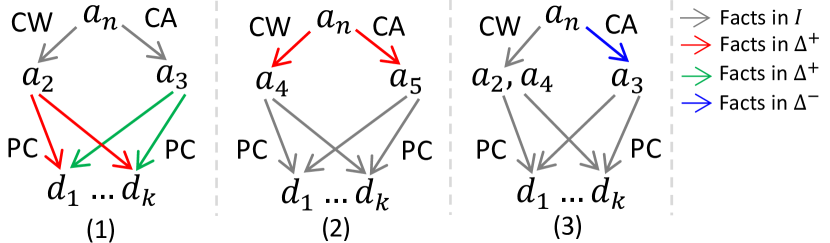
Figure 2: The illustrations depict joins in three scenarios: (1) the second round of rule evaluation; (2) the incremental rule evaluation in response to the addition of $\mathsf{CW}(a_{n},a_{4})$ and $\mathsf{CA}(a_{n},a_{5})$; and (3) the incremental rule evaluation in response to the removal of $\mathsf{CA}(a_{n},a_{3})$. From these joins, one can easily compute the corresponding instantiations for nodes $p_{1}$ and $p_{2}$.

To further elucidate the algorithmic process, we will build upon the examples presented in Section 3 to demonstrate our algorithm’s recursive application in a step-by-step manner.

Example 1.

Following the initial round of rule application as detailed in Section 3, the instantiations in $\mathsf{inst}_{p_{1}}^{I\,\begin{subarray}{c}\cdot\\[-3.41418pt] \cdot\\[-3.41418pt] \cdot\\[1.42271pt] \end{subarray}\,\Delta^{+}}$ and $\mathsf{inst}_{p_{2}}^{I\,\begin{subarray}{c}\cdot\\[-3.41418pt] \cdot\\[-3.41418pt] \cdot\\[1.42271pt] \end{subarray}\,\Delta^{+}}$ are derived in line 3 of algorithm 3 and then merged into $\mathsf{inst}_{p_{1}}^{I}$ and $\mathsf{inst}_{p_{2}}^{I}$ in line 8, respectively, before being cleared in line 9. Therefore, we have ${\mathsf{inst}_{p_{1}}^{I}=\{(a_{i},b_{i\cdot k+j},d_{j})\mid 0\leq i<n,\;1\leq j\leq k\}}$, and $\mathsf{inst}_{p_{2}}^{I}=\{(a_{i},c_{i\cdot k+j},d_{j})\mid 0\leq i<n,\;1\leq j\leq k\}$. Additionally, the cross-node evaluation in line 5 derives facts ${\{\mathsf{PC}(a_{i},d_{j})\mid 0\leq i<n,\;1\leq j\leq k\}}$, which are all returned in line 10 of the algorithm.

In the second round of application, the facts derived in the first round, i.e., $\mathsf{PC}(a_{i},d_{j})$ with $0\leq i<n$ and $1\leq j\leq k$, are passed to the $\mathsf{Add}^{r}$ function as $\Delta^{+}$. Then, line 3 identifies for $p_{1}$ the new instantiations involving facts in $\Delta^{+}$; specifically, $\{(a_{n},a_{2},d_{j})\mid 1\leq j\leq k\}$ are assigned to $\mathsf{inst}_{p_{1}}^{I\,\begin{subarray}{c}\cdot\\[-3.41418pt] \cdot\\[-3.41418pt] \cdot\\[1.42271pt] \end{subarray}\,\Delta^{+}}$. Similarly, we have $\mathsf{inst}_{p_{2}}^{I\,\begin{subarray}{c}\cdot\\[-3.41418pt] \cdot\\[-3.41418pt] \cdot\\[1.42271pt] \end{subarray}\,\Delta^{+}}$ $=$ $\{(a_{n},a_{3},d_{j})\mid 1\leq j\leq k\}$. For an illustration of the related joins, please refer to figure 2 (1). Then, during the cross-node evaluation, lines 2–5 ensure that when node $p_{1}$ is labeled with $\Delta^{+}$, node $p_{2}$ is labeled with $I$, and so $\mathsf{inst}_{p_{1}}^{I\,\begin{subarray}{c}\cdot\\[-3.41418pt] \cdot\\[-3.41418pt] \cdot\\[1.42271pt] \end{subarray}\,\Delta^{+}}$ is joined with $\mathsf{inst}_{p_{2}}^{I}$, deriving no new fact. In contrast, when node $p_{2}$ is labeled with $\Delta^{+}$, node $p_{1}$ is labeled with $I\cup\Delta^{+}$, and so $\mathsf{inst}_{p_{2}}^{I\,\begin{subarray}{c}\cdot\\[-3.41418pt] \cdot\\[-3.41418pt] \cdot\\[1.42271pt] \end{subarray}\,\Delta^{+}}$ is joined with $\mathsf{inst}_{p_{1}}^{I}$ $\cup$ $\mathsf{inst}_{p_{1}}^{I\,\begin{subarray}{c}\cdot\\[-3.41418pt] \cdot\\[-3.41418pt] \cdot\\[1.42271pt] \end{subarray}\,\Delta^{+}}$, deriving $\mathsf{PC}(a_{n},d_{j})$ with $1\leq j\leq k$. As one can readily see, the second round of rule application does not repeat work already carried out in the first round.

The above example demonstrates the process of initial materialisation. Now consider adding $\{\mathsf{CW}(a_{n},a_{4})$, $\mathsf{CA}(a_{n},a_{5})\}$ to the explicitly given data, i.e., by setting $E^{+}$ to the above set of facts in the DRed algorithm. In this case, $\Delta^{+}$ in $\mathsf{Add}^{r}$ will consist of $\mathsf{CW}(a_{n},a_{4})$ and $\mathsf{CA}(a_{n},a_{5})$. Then, in line 3 of algorithm 3, we clearly have $\Pi_{p_{1}}[I,\Delta^{+}]=\{(a_{n},a_{4},d_{j})\mid 1\leq j\leq k\}$, as illustrated by figure 2 (2). However, $\mathsf{inst}_{p_{1}}^{I\,\begin{subarray}{c}\cdot\\[-3.41418pt] \cdot\\[-3.41418pt] \cdot\\[1.42271pt] \end{subarray}\,\Delta^{+}}$ will be empty since the identified instantiations already exist in $\mathsf{inst}_{p_{1}}^{I}$; the same applies to $p_{2}$. As a result, no new fact is derived. This shows the benefit of keeping instantiations for the nodes of the decomposition between different runs of the DRed algorithm.

Algorithm 4 $\mathsf{CrossNodeEvaluation}^{r}(\mathsf{L})$

1:$\Delta:=\emptyset$

2:for $p_{i}\in N^{r}$ do /* the $\Delta$ node */

3:     for $p_{j}\in N^{r}$ do

4:         $\text{label }p_{j}\text{ with the output of }\mathsf{L}(p_{i},p_{j})$

5:         set $\mathsf{inst}_{p_{j}}^{ac}$ according to the label      

6:     $\mathsf{TopDownLSJ}(p_{i})$

7:     $\mathsf{BottomUpLSJ}(t^{r})$; $\mathsf{TopDownLSJ}(t^{r})$

8:     $\Delta:=\Delta\cup\pi_{\mathsf{var(h}(r))}(\mathsf{CrossNodeJoin}(t^{r}))$

9:return $\Delta$

Deletion: The $\mathsf{Del}^{r}$ algorithm shown in algorithm 5 is analogous to $\mathsf{Add}^{r}$, and it identifies consequences of $r$ that are affected by the deletion of $\Delta^{-}$. The algorithm first computes the overdeletion $\mathsf{inst}_{p}^{I\,\begin{subarray}{c}\cdot\\[-3.41418pt] \cdot\\[-3.41418pt] \cdot\\[1.42271pt] \end{subarray}\,\Delta^{-}}$ using the operator $\Pi_{p}$ in lines 2–3. In addition, the instantiations that have been overdeleted are also added to $\mathsf{inst}_{p}^{re}$ so that they can be checked and potentially recovered during rederivation.

The cross-node evaluation in line 6 is similar to that of $\mathsf{Add}^{r}$, except that a different labelling function $\mathsf{L}^{-}$ is used:

$$\mathsf{L}^{-}(p_{i},p_{j})=\left\{\begin{array}[]{lr}I,&p_{j}\prec p_{i}\\ \Delta^{-},&p_{j}=p_{i}\\ I\backslash\Delta^{-},&p_{j}\succ p_{i}\end{array}.\right.$$ (10)

Note that the initialisation of $\mathsf{inst}_{p_{j}}^{ac}$ follows equation (9). Finally, for each node $p$, the set of instantiations $\mathsf{inst}_{p}^{I}$ is updated in line 9 to reflect the change, and $\mathsf{inst}_{p}^{I\,\begin{subarray}{c}\cdot\\[-3.41418pt] \cdot\\[-3.41418pt] \cdot\\[1.42271pt] \end{subarray}\,\Delta^{-}}$ is emptied in line 10 for later use. Similarly as in $\mathsf{Add}^{r}$, our $\mathsf{Del}^{r}$ function exploits the idea of seminaïve evaluation to avoid repeated reasoning. Lemma 2 states that the algorithm is correct.

Lemma 2.

Algorithm 5 computes ${r[I\,\begin{subarray}{c}\cdot\\[-3.41418pt] \cdot\\[-3.41418pt] \cdot\\[1.42271pt] \end{subarray}\,\Delta^{-}]\cap(I\backslash\Delta^{-})}$.

Algorithm 5 $\mathsf{Del}^{r}[I,\Delta^{-}]$

1:/* in-node: overdelete */

2:for $p\in N^{r}$ do:

3:     $\mathsf{inst}_{p}^{I\,\begin{subarray}{c}\cdot\\[-3.41418pt] \cdot\\[-3.41418pt] \cdot\\[1.42271pt] \end{subarray}\,\Delta^{-}}:=\Pi_{p}[I,\Delta^{-}]\cap\mathsf{inst}_{p}^{I}$

4:     $\mathsf{inst}_{p}^{re}:=\mathsf{inst}_{p}^{re}\cup\mathsf{inst}_{p}^{I\,\begin{subarray}{c}\cdot\\[-3.41418pt] \cdot\\[-3.41418pt] \cdot\\[1.42271pt] \end{subarray}\,\Delta^{-}}$

5:/* cross-node: overdelete */

6:$\Delta_{D}:=\mathsf{CrossNodeEvaluation}^{r}(\mathsf{L^{-}})$

7:/* updating instantiations for each node */

8:for $p\in N^{r}$ do

9:     $\mathsf{inst}_{p}^{I}:=\mathsf{inst}_{p}^{I}\backslash\mathsf{inst}_{p}^{I\,\begin{subarray}{c}\cdot\\[-3.41418pt] \cdot\\[-3.41418pt] \cdot\\[1.42271pt] \end{subarray}\,\Delta^{-}}$

10:     $\mathsf{inst}_{p}^{I\,\begin{subarray}{c}\cdot\\[-3.41418pt] \cdot\\[-3.41418pt] \cdot\\[1.42271pt] \end{subarray}\,\Delta^{-}}:=\emptyset$

11:return $\Delta_{D}\cap(I\backslash\Delta^{-})$

The following example illustrates overdeletion using our customised algorithms.

Example 2.

Assume that $E^{-}$ is set as $\{\mathsf{CA}(a_{n},a_{3})\}$ in algorithm 2. During the overdeletion phase, $E^{-}$ is passed to $\mathsf{Del}^{r}$ as $\Delta^{-}$. After the execution of line 3 in algorithm 5, we have $\mathsf{inst}_{p_{2}}^{I\,\begin{subarray}{c}\cdot\\[-3.41418pt] \cdot\\[-3.41418pt] \cdot\\[1.42271pt] \end{subarray}\,\Delta^{-}}$ $=\{(a_{n},a_{3},d_{j})\mid 1\leq j\leq k\}$ and $\mathsf{inst}_{p_{1}}^{I\,\begin{subarray}{c}\cdot\\[-3.41418pt] \cdot\\[-3.41418pt] \cdot\\[1.42271pt] \end{subarray}\,\Delta^{-}}$ $=\emptyset$, as can be seen from figure 2 (3). Then, the cross-node evaluation will derive $\mathsf{PC}(a_{n},d_{j})$, $1\leq j\leq k$. These facts are temporarily overdeleted, and the rederivation stage will check whether they have alternative derivations from the remaining facts.

Rederivation: The rederivation step described in algorithm 6 aims at recovering facts that are overdeleted but are one-step rederivable from the remaining facts using rule $r$. In the presentation of the algorithm we take advantage of an oracle function $\mathsf{O}$ which serves the purpose of encapsulation. The oracle function can be implemented arbitrarily, as long as it satisfies the following requirement: given a fact/tuple $f$, the oracle function returns true if $f$ has a one-step derivation from the remaining facts/tuples, and it returns false otherwise.

In practice, there are several ways to implement such an oracle function. A straightforward way is through query evaluation. For example, to check whether a tuple $f\in\mathsf{inst}_{p}^{re}$ is one-step rederivable, one can construct a query using atoms in ${\lambda(p)}$, instantiate the query with the corresponding constants in $f$, and then evaluate the partially instantiated query over the remaining facts. A more advanced approach is through tracking derivation counts (Hu et al., 2018): each tuple is associated with a number that indicates how many times it is derived; during reasoning, this count is incremented if a new derivation is identified, and it is decremented if a derivation no longer holds. Then, the oracle function can be realised with a simple check on the derivation count of the relevant tuple. We have adopted the second approach in this paper.

Algorithm 6 proceeds as follows. First, lines 1–2 perform rederivation for in-node evaluation using the oracle. Recall that rule evaluation is decomposed into in-node evaluation and cross-node evaluation stages, so changes in the join results stored in the tree nodes have to be propagated through the decomposition tree, and this is achieved through line 3. Then, lines 4–6 update the join results and clear temporal variables. Finally, line 7 performs rederivation for cross-node evaluation and returns all the rederived facts. Lemma 3 states that the algorithm is correct. Together with Theorem 1 and Lemmas 1 and 2, this ensures the correctness of our approach.

Lemma 3.

Algorithm 6 computes ${r[I]\cap\Delta}$.

Below we continue with our running example and focus on the rederivation stage.

Example 3.

After the overdeletion in Example 2, we have $\mathsf{inst}_{p_{2}}^{re}=\{(a_{n},a_{3},d_{j})\mid 1\leq j\leq k\}$. These instantiations will not be recovered in line 2 of algorithm 6 since the oracle $O$ will find out that they have no alternative derivation from the remaining data. In contrast, the overdeleted facts $\mathsf{PC}(a_{n},d_{j})$ with $1\leq j\leq k$ are recovered in line 7. This is so since each $\mathsf{PC}(a_{n},d_{j})$ can be rederived using instantiation $(a_{n},a_{2},d_{j})$ from $\mathsf{inst}_{p_{1}}^{I}$ and instantiation $(a_{n},a_{5},d_{j})$ from $\mathsf{inst}_{p_{2}}^{I}$. These rederived triples are passed on to $\mathsf{Add}^{r}$ as $\Delta^{+}$, but no new fact will be derived. Overall, the removal of $\{\mathsf{CA}(a_{n},a_{3})\}$ do not affect the materialisation.

Algorithm 6 $\mathsf{Red}^{r}[I,\Delta]$

1:for $p\in N^{r}$ do

2:     $\mathsf{inst}_{p}^{I\,\begin{subarray}{c}\cdot\\[-3.41418pt] \cdot\\[-3.41418pt] \cdot\\[1.42271pt] \end{subarray}\,\Delta^{+}}:=\{f\in\mathsf{inst}_{p}^{re}\ |\ \mathsf{O}[f]=\mathsf{true}\}$

3:$\Delta_{R}:=\mathsf{CrossNodeEvaluation}^{r}(\mathsf{L^{+}})\cap\Delta$

4:for $p\in N^{r}$ do

5:     $\mathsf{inst}_{p}^{I}:=\mathsf{inst}_{p}^{I}\cup\mathsf{inst}_{p}^{I\,\begin{subarray}{c}\cdot\\[-3.41418pt] \cdot\\[-3.41418pt] \cdot\\[1.42271pt] \end{subarray}\,\Delta^{+}}$

6:     $\mathsf{inst}_{p}^{re}:=\mathsf{inst}_{p}^{I\,\begin{subarray}{c}\cdot\\[-3.41418pt] \cdot\\[-3.41418pt] \cdot\\[1.42271pt] \end{subarray}\,\Delta^{+}}:=\emptyset$

7:return $\Delta_{R}\cup\{f\in\Delta\ |\ \mathsf{O}[f]=\mathsf{true}\}$

5 Implementation and Evaluation

Benchmarks	$|E|$	$|I|$	$|\Pi|$	$|\Pi_{s}|$	$|\Pi_{c}|$
LUBM L	66,751,196	91,128,727	98	98	0
LUBM L+C	66,751,196	99,361,809	114	98	16
Exp	3,362,280	6,440,280	3	0	3
YAGO	58,276,868	59,755,990	23	0	23

Table 1: Dataset statistics. $|\Pi_{s}|$ and $|\Pi_{c}|$ refer to the numbers of simple and complex rules, respectively.

Method	materialisation				small deletions				large deletions				small additions
	L+C	L	Exp	YAGO	L+C	L	Exp	YAGO	L+C	L	Exp	YAGO	L+C	L	Exp	YAGO
standard	29,577.90	95.73	7,039.87	155,022.00	0.92	0.03	37.60	20.06	15,193.70	27.09	4,006.44	126,562.00	0.97	0.02	40.23	20.42
HD	1,168.83	740.81	56.83	367.59	4.00	3.70	0.47	0.18	812.32	558.90	30.93	168.34	1.04	0.45	0.57	0.17
combined	554.00	75.50	57.01	366.03	1.06	0.04	0.45	0.20	195.51	21.71	28.62	159.43	0.73	0.06	0.53	0.17

Table 2: Materialisation and incremental reasoning time in seconds

To evaluate our algorithms we have developed a proof-of-concept implementation and conducted several experiments.

Implementation: The algorithms presented in Section 4 are independent of the choice of decompositions; however, different hypertree decompositions will lead to very different performance even if they share the same hypertree width. This is because the decomposition method only considers structural information of the queries and ignores quantitative information of the data. To address this problem, Scarcello et al. (2007) introduced an algorithm that chooses the optimal decomposition w.r.t. a given cost model. We adopt this algorithm with a cost model consisting of two parts: (1) an estimate of the cost of intra-node evaluation, i.e., the joins among $\lambda(p)$; and (2) an estimate of the cost of inter-node evaluation, i.e., the joins between nodes. In our implementation, for (1), we use the standard textbook cardinality estimator described in Chapter 16.4 of the book (Garcia-Molina, 2008) to estimate the cardinality of $\underset{B_{i}\in\lambda(p)}{\large\bowtie}B_{i}$ for a node $p$; for (2), we use $2*(|\hat{p_{i}}|+|\hat{p_{j}}|)$ to estimate the cost of performing semi-joins between nodes $p_{i}$ and $p_{j}$, where $|\hat{p_{i}}|$ and $|\hat{p_{j}}|$ represent the estimated node size.

Moreover, the extra step of full reducer we introduced in algorithm 4 (line 6) is more suitable for small updates, in which the node with the smallest size helps reduce other large nodes. If the size of all the nodes is comparable, then this step would be unnecessary. Therefore, in practice, we only perform this optimisation if the number of active instantiations in the $\Delta$ node (i.e., $p_{i}$) is more than three times smaller than the maximum number of active instantiations in each node.

Benchmarks: We tested our system using the well-known LUBM and YAGO benchmarks (Guo et al., 2005; Suchanek et al., 2008), and a synthetic Exp (expressions) benchmark which we created to capture complex rule patterns that commonly occur in practice. LUBM models a university domain, and it includes a data generator that can create datasets of varying sizes; we used the LUBM-500 dataset which includes data for 500 universities. Since the ontology of LUBM is not in OWL 2 RL, we use the LUBM L variant created by Zhou et al. (2013). The LUBM L rules are very simple, so we added 16 rules that capture more complex but semantically reasonable relations in the domain; some of these rules are rewritten from the cyclic queries used by Stefanoni et al. (2018); we call the resulting rule set LUBM L+C. One example rule is $\mathsf{SA}(?p_{1},?p_{2})\leftarrow\mathsf{HA}(?o.?p_{1}),\mathsf{AD}(?p_{1},?ad),\mathsf{HA}(?o,?p_{2}),\mathsf{AD}(?p_{2},?ad)$, in which $\mathsf{HA}$ and $\mathsf{AD}$ represent predicates $\mathsf{hasAlumnus}$ and $\mathsf{hasAdvisor}$ respectively, while $\mathsf{SA}$ in the head represents a new predicate $\mathsf{haveSameAdvisor}$ that links pairs of students $?p_{1}$ and $?p_{2}$ (not necessarily distinct) who are from the same university $?o$ and share the same advisor $?ad$.

YAGO is a real-world RDF dataset with general knowledge about movies, people, organisations, cities, and countries. We rewrote 23 cyclic queries with different topologies (i.e., cycle, clique, petal, flower) used by Park et al. (2020) into 19 non-recursive rules and 4 recursive rules. These rules are helpful to evaluate the performance of our algorithm on topologies that are frequently observed in real-world graph queries (Bonifati et al., 2017).

As mentioned in Section 1, realistic applications often involve complex rules. One example is the use of rules to evaluate numerical expressions, and our Exp benchmark has been created to simulate such cases. Specifically, Exp applies Datalog rules to evaluate expression trees of various depths. It contains three recursive rules capturing the arithmetical operations addition, subtraction and multiplication; each of these rules is cyclic and contains 9 body atoms. A generator is used to create data for a given number of expressions, sets of values and maximum depth. In our evaluation we generated 300 expressions, each with 300 values and a maximum depth of 5. Details of the three benchmarks are given in Table 1, where $|E|$ is the number of given facts, $|I|$ is the number of facts in the materialisation, and $|\Pi|$, $|\Pi_{s}|$, $|\Pi_{c}|$ are the numbers of rules, simple rules, and complex rules, respectively.

Compared Approaches: We considered three different approaches. The standard approach uses the seminaïve algorithm for materialisation and an optimised variant of DRed for incremental maintenance. The HD approach uses our hypertree decomposition based algorithms. The combined approach applies HD algorithms to complex rules and standard algorithms to the remaining rules. To ensure fairness, all three approaches are implemented on top of the same code base obtained from the authors of the modular reasoning framework  (Hu et al., 2022). The framework allows us to partition a program into modules and apply custom algorithms to each module as required.

Test Setups: All of our experiments are conducted on a Dell PowerEdge R730 server with 512GB RAM and 2 Intel Xeon E5-2640 2.60GHz processors, running Fedora 33, kernel version 5.10.8. We evaluate the running time of materialisation (the initial materialisation with all the explicitly given facts inserted as $E^{+}$ in Algorithm 2), small deletions (randomly selecting 1,000 facts from the dataset as $E^{-}$ in Algorithm 2), large deletions (randomly selecting 25% of the dataset as $E^{-}$), and small additions (adding 1,000 facts as $E^{+}$ into the dataset). Materialisation can be regarded as a large addition.

Analysis: The experimental results are shown in Table 2 in which L and L+C are short for LUBM L and LUBM L+C respectively. The computation of decompositions takes place during initial materialisation only and the time taken is included in the materialisation time reported in Table 2; it takes less than 0.05 seconds in all cases. As can be seen, the combined approach outperforms the other approaches in most cases, sometimes by a large factor, and it is slower than the standard approach only for some of the small update tasks on LUBM L and L+C where processing time is generally small. In contrast, the standard approach performs poorly when complex rules are included (i.e., L+C, YAGO, and Exp), while the HD approach performs poorly on the simple rules in LUBM L. In particular, our combined approach is 75-139x faster than the standard approach for all the tasks on Exp; on YAGO, it is 100-793x faster. Moreover, for the materialisation and large deletion tasks on LUBM L+C, the combined approach is about 53x and 77x faster than the standard approach, respectively. Furthermore, for the small deletion and addition tasks on LUBM L+C and all the tasks on LUBM L, our combined method achieves a comparable result with the standard approach. The combined approach performs similarly to the standard approach on LUBM L, as the HD module is never invoked (there are no cyclic rules), and it performs similarly to the HD approach on Exp and YAGO, as the HD module is always invoked (all rules are cyclic). Our evaluation illustrates the benefit of the hypertree decomposition-based algorithms when processing complex rules, and it shows that by combining HD algorithms with standard reasoning algorithms in a modular framework we can enjoy this benefit without degrading performance in cases where some or all of the rules are relatively simple.

Finally, the HD algorithms have to maintain auxiliary data structures for rule evaluation, which incurs some space overhead when the HD module is invoked. Specifically, our combined method consumes up to 2.3 times the memory consumed by the standard algorithm; the detailed memory consumption for each setting can be found in the technical report (Zhang et al., 2023).

6 Related Work

HD in Query Answering: The HD methods have been used in database systems to optimise the performance of query answering. For RDF workload, Aberger et al. (2016) evaluated empirically the use of HD combined with worst-case optimal join algorithms, showing up to 6x performance advantage on bottleneck cyclic RDF queries. Also, in the EmptyHeaded (Aberger et al., 2017) relational engine, a query compiler has been implemented to choose the order of attributes in multiway joins based on a decomposition. This line of work focuses on optimising the evaluation of a single query, while our work focuses on evaluating recursive Datalog rules. For a more comprehensive review of HD techniques for query answering, please refer to Gottlob et al. (2016).

HD in Answer Set Programming: Jakl et al. (2009) applied HD techniques to the evaluation of propositional answer set programs. Assuming that the treewidth of a program is fixed as a constant, they devise fixed-parameter tractable algorithms for key ASP problems including consistency checking, counting the number of answer sets of a program, and enumerating such answers. In contrast to our work, their research focuses on propositional answer set programs.

For ASP in the non-ground setting, a program is usually grounded first, and then a solver deals with the ground instances. The usage of (hyper)tree decomposition has been investigated to decrease the size of generated ground rules in the grounding phase (Bichler et al., 2020; Calimeri et al., 2019). Bichler et al. (2020) used hypertree decomposition as a guide to rewrite a larger rule into several smaller rules, thus reducing the number of considered groundings; Calimeri et al. (2019) studied several heuristics that could predict in advance whether a decomposition is beneficial. In contrast, our work focuses on the (incremental) evaluation directly over the decomposition since the decomposition solely cannot avoid the potential blowup during the evaluation of the smaller rules.

7 Perspectives

In this paper, we introduced a hypertree decomposition-based reasoning algorithm, which supports rule evaluation, incremental reasoning, and recursive reasoning. We implemented our algorithm in a modular framework such that the overhead caused by using decomposition is incurred only for complex rules, and demonstrate empirically that this approach is effective on simple, complex and mixed rule sets.

Despite the promising results, we see many opportunities for further improving the performance of the presented algorithms. Firstly, our decomposition remains unchanged once it is fixed. However, as the input data and the materialisation change over time, the initial decomposition may no longer be optimal for rule evaluation. It would be beneficial if the maintenance could be done with the underlying decomposition changing. However, this would be challenging since the data structure in each decomposition node is maintained based on the previous decomposition, and changing the decomposition would require transferring information from the old node to the new one.

Secondly, although the memory usage has been optimised to some extent, intermediate results still take up a significant amount of space. This problem could be mitigated by incrementally computing the final join result without explicitly storing the intermediate results, or by storing only “useful” intermediate results.

Finally, it would be interesting to adapt our work to Datalog extensions, such as Datalog^± (Calì et al., 2011) and DatalogMTL (Walega et al., 2019). This would require introducing mechanisms to process the relevant additional features, such as the existential quantifier in Datalog^± and the use of intervals in DatalogMTL.

See pages 1,2,3,4,5,6 of appendix.pdf

References

- Aberger et al. [2016] Christopher R Aberger, Susan Tu, Kunle Olukotun, and Christopher Ré. Old techniques for new join algorithms: A case study in rdf processing. In 2016 IEEE 32nd International Conference on Data Engineering Workshops (ICDEW), pages 97–102. IEEE, 2016.
- Aberger et al. [2017] Christopher R Aberger, Andrew Lamb, Susan Tu, Andres Nötzli, Kunle Olukotun, and Christopher Ré. Emptyheaded: A relational engine for graph processing. ACM Transactions on Database Systems (TODS), 42(4):1–44, 2017.
- Abiteboul et al. [1995] Serge Abiteboul, Richard Hull, and Victor Vianu. Foundations of databases, volume 8. Addison-Wesley Reading, 1995.
- Alvaro et al. [2010] Peter Alvaro, Tyson Condie, Neil Conway, Khaled Elmeleegy, Joseph M Hellerstein, and Russell Sears. Boom analytics: exploring data-centric, declarative programming for the cloud. In Proceedings of the 5th European conference on Computer systems, pages 223–236, 2010.
- Aref et al. [2015] Molham Aref, Balder ten Cate, Todd J Green, Benny Kimelfeld, Dan Olteanu, Emir Pasalic, Todd L Veldhuizen, and Geoffrey Washburn. Design and implementation of the logicblox system. In Proceedings of the 2015 ACM SIGMOD International Conference on Management of Data, pages 1371–1382, 2015.
- Bellomarini et al. [2018] Luigi Bellomarini, Georg Gottlob, and Emanuel Sallinger. The vadalog system: Datalog-based reasoning for knowledge graphs. arXiv preprint arXiv:1807.08709, 2018.
- Bernstein and Chiu [1981] Philip A Bernstein and Dah-Ming W Chiu. Using semi-joins to solve relational queries. Journal of the ACM (JACM), 28(1):25–40, 1981.
- Bichler et al. [2020] Manuel Bichler, Michael Morak, and Stefan Woltran. lpopt: A rule optimization tool for answer set programming. Fundamenta Informaticae, 177(3-4):275–296, 2020.
- Bonifati et al. [2017] Angela Bonifati, Wim Martens, and Thomas Timm. An analytical study of large sparql query logs. arXiv preprint arXiv:1708.00363, 2017.
- Calì et al. [2011] Andrea Calì, Georg Gottlob, Thomas Lukasiewicz, and Andreas Pieris. Datalog+/-: A family of languages for ontology querying. In Datalog Reloaded: First International Workshop, Datalog 2010, Oxford, UK, March 16-19, 2010. Revised Selected Papers, pages 351–368. Springer, 2011.
- Calimeri et al. [2019] Francesco Calimeri, Simona Perri, and Jessica Zangari. Optimizing answer set computation via heuristic-based decomposition. Theory and Practice of Logic Programming, 19(4):603–628, 2019.
- Carral et al. [2019] David Carral, Irina Dragoste, Larry González, Ceriel Jacobs, Markus Krötzsch, and Jacopo Urbani. Vlog: A rule engine for knowledge graphs. In International Semantic Web Conference, pages 19–35. Springer, 2019.
- Flum et al. [2002] Jörg Flum, Markus Frick, and Martin Grohe. Query evaluation via tree-decompositions. Journal of the ACM (JACM), 49(6):716–752, 2002.
- Garcia-Molina [2008] Hector Garcia-Molina. Database systems: the complete book. Pearson Education India, 2008.
- Gottlob et al. [2002] Georg Gottlob, Nicola Leone, and Francesco Scarcello. Hypertree decompositions and tractable queries. Journal of Computer and System Sciences, 64(3):579–627, 2002.
- Gottlob et al. [2016] Georg Gottlob, Gianluigi Greco, Nicola Leone, and Francesco Scarcello. Hypertree decompositions: Questions and answers. In Proceedings of the 35th ACM SIGMOD-SIGACT-SIGAI Symposium on Principles of Database Systems, pages 57–74, 2016.
- Guo et al. [2005] Yuanbo Guo, Zhengxiang Pan, and Jeff Heflin. Lubm: A benchmark for owl knowledge base systems. Journal of Web Semantics, 3(2-3):158–182, 2005.
- Gupta et al. [1993] Ashish Gupta, Inderpal Singh Mumick, and Venkatramanan Siva Subrahmanian. Maintaining views incrementally. ACM SIGMOD Record, 22(2):157–166, 1993.
- Horrocks et al. [2004] Ian Horrocks, Peter F Patel-Schneider, Harold Boley, Said Tabet, Benjamin Grosof, Mike Dean, et al. Swrl: A semantic web rule language combining owl and ruleml. W3C Member submission, 21(79):1–31, 2004.
- Hu et al. [2018] Pan Hu, Boris Motik, and Ian Horrocks. Optimised maintenance of datalog materialisations. In Proceedings of the AAAI Conference on Artificial Intelligence, volume 32, 2018.
- Hu et al. [2022] Pan Hu, Boris Motik, and Ian Horrocks. Modular materialisation of datalog programs. Artificial Intelligence, 308:103726, 2022.
- Jakl et al. [2009] Michael Jakl, Reinhard Pichler, and Stefan Woltran. Answer-set programming with bounded treewidth. In IJCAI, volume 9, pages 816–822, 2009.
- Luteberget et al. [2016] Bjørnar Luteberget, Christian Johansen, and Martin Steffen. Rule-based consistency checking of railway infrastructure designs. In International Conference on Integrated Formal Methods, pages 491–507. Springer, 2016.
- Motik et al. [2009] Boris Motik, Peter F Patel-Schneider, Bijan Parsia, Conrad Bock, Achille Fokoue, Peter Haase, Rinke Hoekstra, Ian Horrocks, Alan Ruttenberg, Uli Sattler, et al. Owl 2 web ontology language: Structural specification and functional-style syntax. W3C recommendation, 27(65):159, 2009.
- Motik et al. [2015] Boris Motik, Yavor Nenov, Robert Piro, and Ian Horrocks. Incremental update of datalog materialisation: the backward/forward algorithm. In Proceedings of the AAAI Conference on Artificial Intelligence, volume 29, 2015.
- Motik et al. [2019] Boris Motik, Yavor Nenov, Robert Piro, and Ian Horrocks. Maintenance of datalog materialisations revisited. Artificial Intelligence, 269:76–136, 2019.
- Nenov et al. [2015] Yavor Nenov, Robert Piro, Boris Motik, Ian Horrocks, Zhe Wu, and Jay Banerjee. Rdfox: A highly-scalable rdf store. In International Semantic Web Conference, pages 3–20. Springer, 2015.
- Ngo et al. [2014] Hung Q Ngo, Christopher Ré, and Atri Rudra. Skew strikes back: New developments in the theory of join algorithms. ACM SIGMOD Record, 42(4):5–16, 2014.
- Park et al. [2020] Yeonsu Park, Seongyun Ko, Sourav S Bhowmick, Kyoungmin Kim, Kijae Hong, and Wook-Shin Han. G-care: A framework for performance benchmarking of cardinality estimation techniques for subgraph matching. In Proceedings of the 2020 ACM SIGMOD International Conference on Management of Data, pages 1099–1114, 2020.
- Scarcello et al. [2007] Francesco Scarcello, Gianluigi Greco, and Nicola Leone. Weighted hypertree decompositions and optimal query plans. Journal of Computer and System Sciences, 73(3):475–506, 2007.
- Staudt and Jarke [1995] Martin Staudt and Matthias Jarke. Incremental maintenance of externally materialized views. Citeseer, 1995.
- Stefanoni et al. [2018] Giorgio Stefanoni, Boris Motik, and Egor V Kostylev. Estimating the cardinality of conjunctive queries over rdf data using graph summarisation. In Proceedings of the 2018 World Wide Web Conference, pages 1043–1052, 2018.
- Subercaze et al. [2016] Julien Subercaze, Christophe Gravier, Jules Chevalier, and Frederique Laforest. Inferray: fast in-memory rdf inference. In VLDB, volume 9, 2016.
- Suchanek et al. [2008] Fabian M Suchanek, Gjergji Kasneci, and Gerhard Weikum. Yago: A large ontology from wikipedia and wordnet. Journal of Web Semantics, 6(3):203–217, 2008.
- Tu and Ré [2015] Susan Tu and Christopher Ré. Duncecap: Query plans using generalized hypertree decompositions. In Proceedings of the 2015 ACM SIGMOD International Conference on Management of Data, pages 2077–2078, 2015.
- Walega et al. [2019] Przemyslaw Andrzej Walega, B Cuenca Grau, Mark Kaminski, and Egor V Kostylev. Datalogmtl: Computational complexity and expressive power. International Joint Conferences on Artificial Intelligence, 2019.
- Wu et al. [2008] Zhe Wu, George Eadon, Souripriya Das, Eugene Inseok Chong, Vladimir Kolovski, Melliyal Annamalai, and Jagannathan Srinivasan. Implementing an inference engine for rdfs/owl constructs and user-defined rules in oracle. In 2008 IEEE 24th International Conference on Data Engineering, pages 1239–1248. IEEE, 2008.
- Yannakakis [1981] Mihalis Yannakakis. Algorithms for acyclic database schemes. In VLDB, volume 81, pages 82–94, 1981.
- Zhang et al. [2023] Xinyue Zhang, Pan Hu, Yavor Nenov, and Ian Horrocks. Enhancing datalog reasoning with hypertree decompositions. CoRR, abs/2305.06854, 2023.
- Zhou et al. [2013] Yujiao Zhou, Bernardo Cuenca Grau, Ian Horrocks, Zhe Wu, and Jay Banerjee. Making the most of your triple store: query answering in owl 2 using an rl reasoner. In Proceedings of the 22nd international conference on World Wide Web, pages 1569–1580, 2013.