Stochastic Variance-Reduced Majorization-Minimization Algorithms
Abstract
We study a class of nonconvex nonsmooth optimization problems in which the objective is a sum of two functions: One function is the average of a large number of differentiable functions, while the other function is proper, lower semicontinuous and has a surrogate function that satisfies standard assumptions. Such problems arise in machine learning and regularized empirical risk minimization applications. However, nonconvexity and the large-sum structure are challenging for the design of new algorithms. Consequently, effective algorithms for such scenarios are scarce. We introduce and study three stochastic variance-reduced majorization-minimization (MM) algorithms, combining the general MM principle with new variance-reduced techniques. We provide almost surely subsequential convergence of the generated sequence to a stationary point. We further show that our algorithms possess the best-known complexity bounds in terms of gradient evaluations. We demonstrate the effectiveness of our algorithms on sparse binary classification problems, sparse multi-class logistic regressions, and neural networks by employing several widely-used and publicly available data sets.
Keywords— Majorization-minimization, surrogate functions, variance reduction techniques
1 Introduction
We focus on a class of nonsmooth and nonconvex problems of the form
| (1) |
where is a proper and lower semicontinuous function, and has a large-sum structure, that is,
| (2) |
where is differentiable (possibly nonconvex). The large-sum structure captures, in particular, regularized empirical risk, where represents a loss function on a single data point and is often a nonsmooth (possibly nonconvex) function that regularizes the promotion of sparse solutions, such as -norm, Geman [16], MCP [51], log-sum penalty [8], and exponential concave penalty [7]. Thus, problem (1) models a broad range of optimization problems from convex (i.e., and are convex functions), such as logistic regression, to fully nonconvex problems (i.e., both and are nonconvex) such as optimizing deep neural networks. Since nonconvex optimization became indispensable in recent advances in machine learning models, we focus our attention on the fully nonconvex scenario in problem (1). Specifically, we are interested in the case where the number of components is extremely large since it is a key challenge in the era of big data applications.
1.1 Motivation and Related Work
In the convex setting, a standard method for solving the non-composite form () of problem (1) is the gradient descent method (GD). Given an initial point , the iterative step of the GD method computes by
where is a stepsize. In (2), if the number of components is very large, each iteration of the GD method becomes extremely expensive since it requires the computation of the gradient for all of the components . An effective alternative is the standard stochastic gradient method (SGD) [43]. In this case, in each iteration, the SGD draws randomly from , and updates by
The advantage of the SGD method is that in each iteration, it only evaluates the gradient of a single component function. Consequently, the computational cost per iteration is only of that of the full step in the GD method. However, due to the variance, inadvertently generated by random sampling, the SGD method converges much slower than the full GD method. Fortunately, we can overcome this drawback by variance-reduction techniques, utilizing information regarding the gradient from previous iterations to construct a better estimation of the gradient at the current step. To date, some of the most widely applied variance reduction methods in the literature are the stochastic average gradient algorithm (SAGA) [12], the stochastic variance reduced gradient (SVRG) [21], and the stochastic average gradient (SAG) [48]. We note in passing that SAGA is an unbiased version of SAG. Variance reduction methods inherit the advantage of low iteration cost of the SGD method while providing similar convergence rates of the full GD method in convex settings.
Thus far, however, only several variance reduction methods have been developed in order to deal with nonconvex optimization problems possessing the large-sum structure. Furthermore, these methods mainly focus on special cases of (1), where , such as [1, 2, 37], or where is convex, such as [20, 29]. For the fully nonconvex problem with an extremely large value of (such as we study here), such developments become even more challenging. Consequently, research in this direction is sparse. Several recent studies, such as [30, 49, 27, 28] promote stochastic methods based on difference-of-convex (DC) algorithm, developed in [26, 41], or majorization minimization (MM), developed in [25]. In particular, if is -smooth and has a DC structure, that is, with being proper lower semicontinuous convex and being convex, problem (1) can be reformulated as a DC program
| (3) |
where and are convex functions with . The classic DC algorithm (DCA) linearizes the function iteratively and updates by
| (4) | ||||
for some .
For convenience, before we continue our discussion, we set the following notations. Throughout, for , we denote by the index batch which is a list of (possibly repeated) indices of fixed size where each index is independently and randomly chosen from . We refer to as a random batch of size . Let . With a sequence and a sequence of batches , we associate for all , and inductively, having defined , we set
| (5) |
In other words, is updated to if and only if .
In [49, 27], a stochastic version of DCA, named SDCA, was studied based on the idea of incrementally linearizing the components of . More specifically, is replaced by the so-called SAG estimator
| (6) |
Consequently, subproblem (4) is replaced by
| (7) |
where for all .
Recently, Le Thi et al. [28] developed stochastic DC algorithms, named DCA-SAGA and DCA-SVRG, based on the so-called SAGA and SVRG estimators for the problem in which is a DC function. Specifically, DCA-SAGA applied to (3) successively replaces in DCA’s subproblem (4) by the SAGA stochastic gradient estimate:
which, when combined with (4), implies that
| (8) | ||||
In comparison, DCA-SVRG replaces in DCA’s subproblem by the SVRG stochastic gradient estimate:
| (9) |
where if , and otherwise, where is a fixed positive integer. Consequently, the corresponding subproblem for DCA-SVRG is
| (10) | ||||
In general, problem (1) can be solved by an MM principle such that at each iteration, a complex objective function is approximated by an upper bound which is created around the current iteration and which can be minimized effectively. This step is called the majorization step. The minimum of this upper bound (the minimization step) is then used to sequentially create another, hopefully, tighter, upper bound (another majorization step) to be minimized. More specifically, the MM scheme applied to (1) computes by
| (11) |
where is an upper bound (or surrogate, see Definition 3.1) of at . Indeed, various deterministic approaches can be interpreted from the MM point of view such as proximal or gradient-based methods [11, 22, 3, 46, 31, 5, 17, 33], and expectation-maximization algorithms in statistics [13, 32]. To date, many extensions of MM have been developed, e.g., [42, 39, 23, 19, 18, 9, 10]. However, only a few algorithms have been applied in the large-sum structure settings. In particular, Mairal [30] introduced the minimization of incremental surrogate (MISO) that applies to problem (1) and successively updates by
| (12) |
where is a surrogate of at . However, in order to study asymptotic convergence, Mairal [30] employs a strong assumption, namely, that the approximation errors are -smooth in . It is noteworthy that although MISO was inspired by SAG (see (6)), it does not recover SAG as a special case for smooth and composite convex optimization.
1.2 Contribution and Organization
For solving problem (1) in the case where it incorporates a large-sum structure and nonconvexity of the objective, we introduce three stochastic variance-reduced majorization-minimization (SVRMM) algorithms:
-
•
MM-SAGA (incorporates the techniques of SAGA);
-
•
MM-SVRG (incorporates loop-less variants of SVRG); and
-
•
MM-SARAH (incorporates loop-less variants of SARAH).
Unlike MISO, the SVRMM iterates on and the large-sum separately. In particular, at each iteration, MM-SAGA, MM-SVRG, and MM-SARAH replace the full gradient of in the deterministic MM by stochastic gradient estimators employing SAGA, loop-less SVRG, and loop-less SARAH, respectively. It is important to note that MM-SAGA updates the proximal term at the current iterate in the same manner as in the MM scheme. This distinguishes MM-SAGA from DCA-SAGA when applied to the DC program (3), where the latter’s update rule consists of the proximal at . In addition, we point out that MM-SVRG employs the loop-less SVRG estimator, which was shown to have superior performance [24] when compared to the classic estimator technique SVRG, employed in DCA-SVRG.
Under mild assumptions, we analyze the subsequential convergence for the generated sequence of the SVRMM algorithms. More concretely, we show that each limit point of the generated sequence is a stationary point of Problem (1). Meanwhile, Le Thi et al. [28] showed that each limit point of the generated sequence by their algorithms DCA-SAGA and DCA-SVRG is a DC critical point of , i.e., , which is weaker than the stationary point property, since . Furthermore, we show that our algorithms have convergence rate with respect to the proximity to a stationary point. In order to obtain an -stationary point, we show that MM-SAGA and MM-SVRG have complexity of while MM-SARAH has complexity of in terms of gradient evaluations. That is, our results are superior to those of DCA-SAGA and DCA-SVRG which have complexity of and , respectively, for finding an -DC critical point. Another advantage of our methods is that we do not impose -smoothness on the function , it may be nonsmooth and nonconvex, but rather, in order to obtain our results, the stochastic DCA based algorithms require that the second DC component of , namely, the component in the decomposition , is -smooth. Table 1 contains a comparison between our new methods and DCA-SAGA and DCA-SVRG for solving nonsmooth nonconvex optimization problems, in terms of the requirement on our stepsize and our batch size , in order to achieve the corresponding complexity.
| Method | Requirement | Stepsize | Batch size | Complexity |
|---|---|---|---|---|
| DCA-SAGA [28] | ||||
| DCA-SVRG [28] | , | |||
| MM-SAGA (new) | ||||
| MM-SVRG (new) | , | |||
| MM-SARAH (new) | , |
In Table 1, the stepsizes and batchsizes of DCA-SAGA and DCA-SVRG are taken from [28], and the stepsizes and batchsizes for the MM-SAGA, MM-SVRG, and MM-SARAH are chosen in order to achieve the optimal order of complexity. We also note by passing that by setting the stepsize , we obtain the same complexity in all three SVRMM algorithms.
Finally, we apply our algorithms to solve three problems: sparse binary classification with nonconvex loss and regularizer, sparse multi-class logistic regression with nonconvex regularizer, and feedforward neural network training, in order to illustrate their applicability and efficiency.
The paper is organized as follows. In Section 2, we present basic concepts and properties in nonconvex optimization. In Section 3, we present our algorithms. We analyze the convergence properties of our methods in Section 4. In Section 5, we provide a demonstration by numerical experiments, followed by conclusions in Section 6.
2 Preliminaries
We follow standard notations such as in [4, 45]. Throughout, denotes the inner product in with induced norm defined by . We set . For a nonempty closed set , the distance of from is defined by . An extended-real-valued function is said to be proper if its domain, the set , is nonempty. We say that is lower semicontinuous if, at each ,
Let . We say that is -convex if is convex, equivalently, if
In particular, is convex if and only if is -convex. In the case where the function is -convex, we say that is -strongly convex if and we say that is -weakly convex if .
Definition 2.1 (Fréchet and limiting subdifferential).
[45, Definition 8.3] Let be a proper lower semicontinuous function.
-
(a)
For each we denote by the Fréchet subdifferential of at . It contains all of the vectors which satisfy
If we set
-
(b)
The limiting-subdifferential of at is defined by
If is convex, then the Fréchet and the limiting subdifferential coincide with the convex subdifferential:
Definition 2.2 (-Lipschitz).
A mapping is said to be -Lipschitz, , if
Definition 2.3 (-smooth).
Let . We say that is -smooth if it is differentiable and its gradient, , is -Lipschitz.
We now recall several useful basic facts.
Lemma 2.4.
Let and be proper and lower semicontinuous. Then,
-
(a)
if attains a local minimum at .
-
(b)
if and is continuously differentiable in a neighborhood of .
-
(c)
if is convex and is defined by
-
(d)
if is -smooth.
Proof.
Definition 2.5 (Stationary point).
We say that a stationary point of if
Definition 2.6 (-stationary point).
A point is said to be an -stationary point of if
The following lemma is a fundamental tool in our convergence analysis.
Lemma 2.7 (Supermartingale convergence [44, Theorem 1]).
Let , and be three sequences of random variables and let be sets of random variables such that for all . Assume that
-
(a)
The random variables , and are nonnegative and are functions of random variables in ;
-
(b)
for each ;
-
(c)
with probability .
Then, , and converges to a nonnegative random variable, almost surely.
3 Stochastic Variance-Reduced Majorization-Minimization
In this section, we introduce three stochastic variance-reduced majorization-minimization (SVRMM) algorithms for solving problem (1). To this end, we define surrogate functions as follows.
Definition 3.1 (Surrogate function).
A function is said to be a surrogate function of if
-
(a)
for all ;
-
(b)
for all .
We introduce our first SVRMM algorithm, which we call MM-SAGA. It combines the deterministic MM and the SAGA-style of stochastic gradient update. In particular, we replace the full gradient in the deterministic MM (11) with the stochastic gradient estimate (13). MM-SAGA is formally detailed in Algorithm 1.
| (14) |
Remark 3.2 (MM-SAGA vs. DCA-SAGA).
The update rule (8) of DCA-SAGA [28] can be expressed as
where and . This update is different from our update rule (14) in MM-SAGA which employs the proximal term , in the same manner as in the deterministic MM.
It is worth mentioning an advantage of MM-SAGA over DCA-SAGA in terms of memory storage, which can be described as follows. For MM-SAGA, one employs solely for computing only. In other words, (13) and (14) are completely defined and updated using only the gradient values. Thus, it suffices to keep only the value , and then discard . In many problems, such as binary classifications and multi-class logistic regressions, each gradient is a scalar multiple of the data point , where the scalar can be updated in each iteration. In such cases, one may only store the weights, instead of the full gradient . In contrast, for DCA-SAGA, in addition to the values of gradients , one must store all vectors in order to compute in each iteration.
Our second SVRMM algorithm, named MM-SVRG, is inspired by a loop-less SVRG estimator. Specifically, we replace the full gradient in the deterministic MM (11) by the loop-less SVRG stochastic gradient estimate (15) (see [24]). MM-SVRG is formally detailed in Algorithm 2.
| (15) |
| (16) |
Remark 3.3.
Our third SVRMM algorithm is named MM-SARAH, in which we replace the gradient in the deterministic MM (11) with a loop-less variant of SARAH (17). MM-SARAH is formally detailed in Algorithm 3.
| (17) |
| (18) |
Finally, for convenience, we summarize all of the algorithms under discussion in the following three tables. First, the gradient estimators are detailed as follows.
The next table details iteration updates for algorithms from the literature.
Finally, iteration updates for our three SVRMM algorithms are summarized in the following table, where is a surrogate function for , see Definition 3.1.
4 Convergence analysis
We now focus on convergence analysis of our SVRMM algorithms. To this end, throughout this paper, we assume the following basic assumptions regarding problem (1). Such assumptions are standard in optimization literature, see, e.g., [34, 40].
Assumption 4.1.
-
(a)
is bounded from below, that is, , and
-
(b)
is continuously differentiable and there exists a positive constant such that
(19)
We note that (19) is satisfied if each component function is -smooth. Indeed, in this case,
which implies that (19) holds with . It is also worth noting that (19) implies -smoothness of . Indeed,
which implies that , i.e., is -smooth.
Our following assumption is regarding the surrogate function of , see Definition 3.1.
Assumption 4.2.
-
(a)
For every , is continuous in .
-
(b)
For every , is lower semicontinuous and convex.
-
(c)
There exists a function such that for every , is continuously differentiable at with , and the approximation error satisfies
(20)
Remark 4.3.
We recall several classes of functions which satisfy Assumption 4.2. In particular, we recall functions with -smooth approximation error such that . Additional examples can be found in [30, 23].
Example 4.4 (Proximal surrogates).
If is -weakly convex, it is natural to consider the surrogate
Example 4.5 (Lipschitz gradient surrogates).
If is -smooth, a natural surrogate is
for some .
Example 4.6 (DC surrogates).
If is a DC function, that is, where is -smooth, we consider the surrogate function
We now provide an example in which the approximation error function is nonsmooth, however, Assumption 4.2 is satisfied.
Example 4.7 (Composite surrogates).
Consider a class of functions of the form
where is decomposed into blocks with , , and where are convex and Lipschitz continuous with a common Lipschitz constant , and are concave and smooth with a common smoothness constant on the image . This class includes composite functions, in particular, several existing sparsity-reduced regularizers, which are nonconvex and nonsmooth approximations of the -norm or -norm, see, e.g., [7, 8]. Since is concave, we can setup a surrogate function for as follows
Since is -smooth on the image , it follows from Lemma 2.4 (d) that
which, when combined with the -Lipschitz continuity of , implies that
Therefore, Assumption 4.2 (c) is satisfied when we set .
The following lemma will be useful in our convergence analysis.
Lemma 4.8.
Let and set . Suppose that is a list of length of (possibly repeated) indices where each is chosen independently and randomly from . Then
| (21) |
where the expectation is taken over all possible choices of .
Proof.
We begin with the observation that
Since are chosen independently and randomly from , then for each pair such that ,
and
By recalling that contains indices, it follows that
which completes the proof. ∎
Before we proceed to our convergence analysis, for simplicity, we associate with each of our algorithms a sequence of random variables , which is defined by
| (22) |
In our analysis, we estimate , where denotes either , or , and denotes the conditional expectation given the history of the sequence up to the iteration . We also provide several properties of the sequence . Our arguments are similar to the arguments in the study [14] of stochastic proximal alternating linearized minimization algorithms using SAGA and SARAH for two-block optimization. However, we consider one block, which yields tighter bounds when compared to the bounds in [14, Proposition 2].
Lemma 4.9.
Proof.
First, we estimate as follows. From the definition of the stochastic gradient estimator (13), it follows that
| (24) | ||||
We note that for each ,
| (25) |
Consequently, Lemma 4.8 implies that
Thus, (a) holds for MM-SAGA. Next, we prove that (b) holds for MM-SAGA. By employing the inequality
| (26) |
we see that
| (27) | |||
| (28) |
where (27) follows from
and (28) follows from Assumption 4.1 (b). By setting , we see that
i.e., (b) holds for MM-SAGA
Next, we show that (a) holds for MM-SVRG. From the definition of and (see (15)), it follows that
We note that for each ,
| (29) |
Consequently, Lemma 4.8 implies that
Finally, we prove that (b) holds for MM-SVRG. Again, by recalling (26), we see that
Consequently, by setting , we arrive at
as asserted. ∎
Lemma 4.10.
Proof.
We now present our main convergence results. The following theorem provides almost surely subsequential convergence of the iterations generated by our algorithms to a stationary point. For simplicity, we set the constant in (33).
| (33) |
Theorem 4.11 (Almost surely subsequential convergence).
Let be a sequence generated by one of the SVRMM algorithms. Suppose that Assumptions 4.1 and 4.2 are satisfied, and that the condition
| (34) |
where and are determined by (23) for MM-SAGA and MM-SVRG, by (30) for MM-SARAH, and is defined by (33), holds. Then
-
(a)
The sequence converges almost surely.
-
(b)
The sequence has a finite sum (in particular, vanishes) almost surely.
-
(c)
Every limit point of is a stationary point of , almost surely.
Proof.
First, we prove (a) and (b). From the definition of a surrogate function (see Definition 3.1), it follows that
| (35) |
By combining the -smoothness of with Lemma 2.4(d), we arrive at
| (36) |
Now, by combining the update rule for with Lemma 2.4(c), we see that
| (37) |
Consequently, by summing up (35), (36), and (37), and by recalling that , we obtain
| (38) |
By taking the expectation in (38), conditioned on , we arrive at
| (39) |
We now consider two cases. One case, in which the sequence is generated by either MM-SAGA or MM-SVRG, and the second case, in which the sequence is generated by MM-SARAH.
Case 1: Suppose that is generated by either MM-SAGA or MM-SVRG. Lemma 4.9 (a) asserts that
which, when combined with inequality (39), implies that
By recalling Lemma 4.9 (b), which asserts that , we obtain
Consequently, by setting , we see that
Case 2: Suppose that is generated by MM-SARAH. It follows from (39) and Lemma 4.10 that
Thus, by setting , we obtain
| (40) |
Consequently, in both cases, (40) holds for the corresponding sequences . Now, since
by setting , we see that
On the other hand, without the loss of generality, we may assume that . Thus, by supermartingale convergence (Lemma 2.7), the sequence almost surely has a finite sum (in particular, it vanishes), and almost surely converges to a nonnegative random variable . Consequently, by combining Lemma 4.9, 4.10, and the supermartingale convergence in Lemma 2.7, has a finite sum (in particular, it vanishes) almost surely. It follows that the sequence converges to almost surely, which concludes the proof of (a) and (b).
Proof of (c): First, we claim that
| (41) |
Indeed, by taking the total expectation in (40), we see that
| (42) |
where . By telescoping (42) over , we arrive at
where we employed the fact that . Consequently, has a finite sum.
We now prove that the claim holds by considering two cases: Case 1, where is generated by either MM-SAGA or MM-SVRG, and case 2, where the sequence is generated by MM-SARAH.
Case 1: Suppose that is generated by either MM-SAGA or MM-SVRG. Lemma 4.9 implies that
| (43) |
By telescoping (43), we see that
| (44) |
where (44) is a consequence of and . The claim now follows from (44) and the fact that has a finite sum.
Case 2: Suppose that is generated by MM-SARAH. Lemma 4.10 implies that
| (45) |
By telescoping (45), we see that
| (46) |
where (46) is a consequence of and . The claim now follows from (46) and the fact that has a finite sum.
This concludes the proof of claim (41).
By combining (41) and part (b), for any sequence generated by one of our SVRMM algorithms,
| (47) |
almost surely. Let be generated by an SVRMM algorithm which satisfies (47). Let be a limit point of , that is, there is a subsequence of such that as . From the update rule of the SVRMM algorithms, it follows that
which implies that for any ,
| (48) |
By plugging into (48) and by letting , we arrive at
| (49) |
where we employed the continuity of in (Assumption 4.2 (a)), the fact that
By combining (49) with the lower semicontinuity of in (Assumption 4.2 (b)), we conclude that
Consequently, by letting in (48), we see that for all ,
| (50) |
On the other hand, since is -smooth,
| (51) |
By summing up (50) and (51), we arrive at
for some function which satisfies Assumption 4.2 (c). Consequently, is a minimizer of
It follows that
| (52) |
which concludes part (c) and completes the proof.
∎
Remark 4.12 (feasibility of the batchsize and the stepsize ).
We now provide iteration complexity in order to obtain an -stationary point. To this end, we incorporate the following additional assumption [19, Assumption 3(ii)] regarding the surrogate function of .
Assumption 4.13.
For any bounded subset of , there exists a constant such that for any and for any , there exists such that .
Remark 4.14.
We consider the case where is -smooth in and , as assumed in [30]. We assert that Assumption 4.13 captures this case. Indeed, since , if , then there exists such that
It follows that the proximal surrogates (Examples 4.4), the Lipschitz gradient surrogates (Examples 4.5), and the DC surrogates (Example 4.6) satisfy Assumption 4.13. Furthermore, Assumption 4.13 captures composite surrogates (Example 4.7) with non-smooth approximation error functions. Indeed, let . Then
On the other hand, it follows from [47, Corollary 5Q] that
Consequently, by letting , we arrive at
which implies that Assumption 4.13 is satisfied by letting .
Theorem 4.15 (Iteration complexity).
Let be a sequence generated by one of the SVRMM algorithms. Suppose that Assumptions 4.1, 4.2, 4.13, and condition (34) are satisfied. Then for any ,
| (53) |
In other words, it takes at most iterations, in expectation, to obtain an -stationary point of .
Proof.
From the update rule of the SVRMM algorithms, it follows that
Thus, by Assumption 4.13, there exists such that . Consequently, by invoking Lemma 2.4 (b), it follows that
We see that
It now follows that
| (54) |
On the other hand, if the sequence is generated by either MM-SAGA or MM-SVRG, Lemma 4.9 implies that
| (55) |
By plugging (55) into (54) we arrive at
| (56) |
Moreover, it follows from (40) that
| (57) |
where . By combining (56) and (57), we see that
| (58) |
Consequently, by telescoping (58) over , we obtain
| (59) |
where (59) follows from , , and . We conclude the proof in the case of MM-SAGA and MM-SVRG by combining (59) and the fact that
| (60) | ||||
| (61) |
where (61) follows from (38) and (60) follows by recalling that
The SVRMM algorithm includes two parameters: and the batch-size . Setting yields a larger stepsize compared to other stochastic gradient methods such as DCA-SAGA and DCA-SVRG [28], with a stepsize of , ProxSVRG [20], with a stepsize of , and ProxSVRG+ [29], with a stepsize of . After fixing , we select the batch-size that satisfies condition (34). The following corollary summarizes choices of the batch size and the associated complexity of each algorithm in terms of the number of individual stochastic gradient valuations .
Corollary 4.16.
-
(a)
In the case of MM-SAGA, we set and . Consequently, the complexity is .
-
(b)
In the case of MM-SVRG, we set , and . Consequently, the complexity is .
-
(c)
In the case of MM-SARAH, we set , and . Consequently, the complexity is .
Remark 4.17.
- (a)
- (b)
5 Numerical experiments
We now examine the applicability and efficiency of our SVRMM algorithms. To this end, we consider the following three problems: sparse binary classification with nonconvex loss and regularizer, sparse multi-class logistic regression with nonconvex regularizer, and feedforward neural network training.
We compare six algorithms:
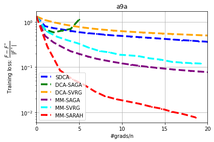
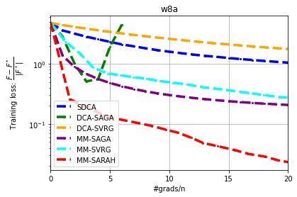
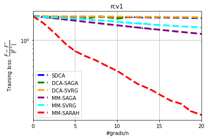
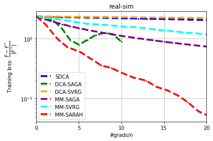
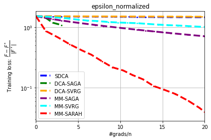
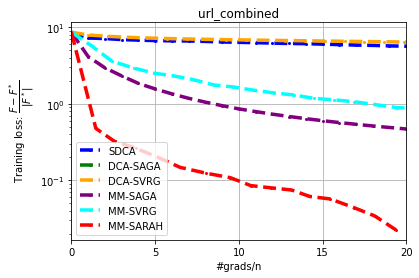
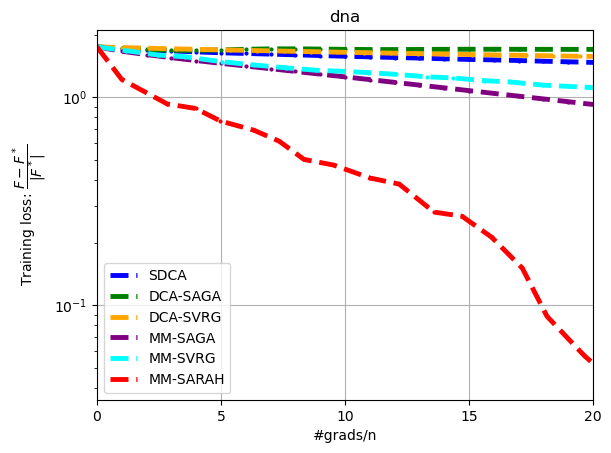
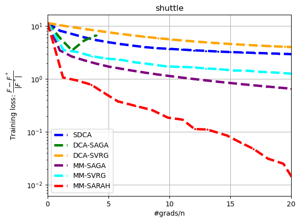
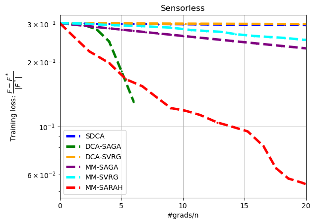
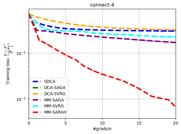
In our experiments, we run each algorithm 20 epochs repeated 20 times, where each epoch consists of gradient evaluations. We are interested in the relative loss residuals , where is the minimum loss values generated by all algorithms, and in classification accuracy on testing sets.
All tests are performed using Python on a Linux server with configuration: Intel(R) Xeon(R) Gold 5220R CPU 2.20GHz of 64GB RAM. The code is available at https://github.com/nhatpd/SVRMM.
5.1 Sparse binary classification with nonconvex loss and regularizer
Let be a training set with observation vectors and labels . We consider the sparse binary classification with nonconvex loss function and nonconvex regularizer:
| (64) |
where is a nonconvex loss function and is a regularization term. We revisit a nonconvex loss function from [52]: , and the exponential regularization from [7]: , where and are the functions
| (65) |
where and are nonnegative tuning parameters. The hessian matrix of is evaluated as follows:
We thus have
Therefore, is -smooth with
and, in this case, problem (64) is within the scope of problem (1) when we let . Moreover, since is concave and -smooth on , and since is convex and -Lipschitz continuous, we set a surrogate function for as follows:
Assumptions 4.2 and 4.13 are then satisfied. The SVRMM algorithms update to be the solution of the nonsmooth convex subproblem:
for which a closed-form solution was provided in [38, Section 6.5.2] by
where .
5.2 Sparse multi-class logistic regression with nonconvex regularizer
We revisit the multi-class logistic regression with a nonconvex regularizer:
| (66) |
where is the number of classes, is a training set with the feature vectors and the labels , is a regularizer, and is a loss function defined by
where is the -th column of . We employ an exponential regularizer, defined by
where is defined as in (65), and is the -th row of . Since is -smooth with , it follows that problem (66) is within the scope of problem (1) when we set . The SVRMM algorithms applied to (66) iteratively determine a surrogate function of at by
and then update by
for which a closed-form solution was provided in [38, Section 6.5.1] by
where .
5.3 Feedforward neural network training problem with nonconvex regularizer
We consider the nonconvex optimization model arising in a feedforward neural network configuration
| (67) |
where all of the weight matrices and bias vectors of the neural network are concatenated in one vector of variables , is a training data set with the feature vectors and the labels , is a composition of linear transforms and activation functions of the form , where is a weight matrix, is a bias vector, is an activation function, is the number of layers, is the soft-max cross-entropy loss, and is a regularizer. By considering the exponential regularization , where and are set in (65), problem (67) is within the scope of of problem (1) when we let . The SVRMM algorithms applied to (67) are different from the SVRMM algorithms for problem (64) only in computation of stochastic gradient estimates . In our experiment, we employ a one-hidden-layer fully connected neural network, , as studied in [40]. The activation function of the hidden layer is ReLU.
5.4 Experiment setups and data sets
In our experiments, for the first two problems (64) and (66), all of the algorithms under study start at the zero point, while for the last problem (67), we use the global_variables_initializer function from Tensorflow. We set the regularization parameters for the first two problems and for the latter, and we fix . These regularization parameters are standard in the literature, e.g., [40, 7]. It is important to mention that in all of the experiments, we use the same problem settings for all of the algorithms.
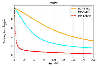
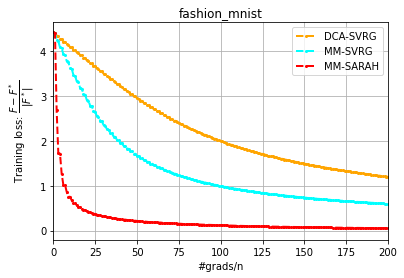
For the sparse binary classification, we carried out the experiments on six different well-known data sets: a9a, w8a, rcv1, real-sim, epsilon, and url. For the sparse multi-class logistic regression, we test all of the algorithms on four data sets: dna, shuttle, Sensorless, and connect-4. Finally, for the feedforward neural network training, we use two data sets minist and fashion_mnist, to compare MM-SVRG and MM-SARAH with DCA-SVRG. We randomly pick 90% of the data for training and the rest for testing. The characteristics of the data sets are provided in Table 2. The first eleven data sets are obtained from the LIBSVM Data website111https://www.csie.ntu.edu.tw/~cjlin/libsvmtools/datasets/ while the data sets minist and fashion_mnist are obtained from the library tensorflow.keras.datasets.
| Data set | Data points | Class number | Feature number |
|---|---|---|---|
| a9a | 32,561 | 2 | 123 |
| w8a | 49,749 | 2 | 300 |
| rcv1-binary | 20,242 | 2 | 47,236 |
| real-sim | 27,309 | 2 | 20,958 |
| epsilon | 400,000 | 2 | 2,000 |
| url | 2,396,130 | 2 | 3,231,961 |
| dna | 2,000 | 11 | 180 |
| shuttle | 43,500 | 7 | 9 |
| Sensorless | 58,509 | 11 | 48 |
| connect-4 | 67,557 | 3 | 126 |
| mnist | 60,000 | 10 | 780 |
| fashion mnist | 60,000 | 10 | 780 |
5.5 Results
We plotted the curves of the average value of relative loss residuals versus epochs in Figures 1-2, and reported the average and the standard deviation of the relative loss residuals and the testing accuracy in Table 3. We observe from Table 3 and Figures 1-2 that MM-SARAH has the fastest convergence on all of the data sets. MM-SARAH achieves not only the best relative loss residuals but also the best classification accuracy on the testing sets. This illustrates the theoretical results, see Corollary 4.16, where MM-SARAH has the best complexity among these algorithms. In addition, MM-SAGA performs better than DCA-SAGA, which is not stable on the first ten data sets. This illustrates the benefit of the proximal term in the iterate of MM-SAGA. Moreover, MM-SVRG performs better than DCA-SVRG on all of the data sets, which illustrates the benefit of the loop-less variant of SVRG in MM-SVRG.
6 Conclusion
We introduced three stochastic variance-reduced MM algorithms: MM-SAGA, MM-SVRG, and MM-SARAH, combining the MM principle and the variance reduction techniques from SAGA, SVRG, and SARAH for solving a class of nonconvex nonsmooth optimization problems with the large-sum structure. The complex objective function is approximated by compatible surrogate functions, providing closed-form solutions in the updates of our algorithms. At the same time, we employ the benefits of the stochastic gradient estimators (SAGA, loop-less SVRG, and loop-less SARAH) to overcome the challenge of the large-sum structure. We provided almost surely subsequential convergence of MM-SAGA, MM-SVRG, and MM-SARAH to a stationary point under mild assumptions. In addition, we proved that our algorithms possess the state-of-the-art complexity bounds in terms of the number of gradient evaluations without assuming that the approximation errors of the regularizer are -smooth. We applied our new algorithms to three important problems in machine learning in order to demonstrate the advantages of combining the MM principle with SAGA, SVRG, and SARAH. Overall, MM-SARAH outperforms other stochastic algorithms under consideration. This is not surprising since the methods based on SAGA and SVRG have unvoidable limitations. In particular, SAGA requires storing the most recent gradient of each component function while SVRG employs a pivot iterate that may be unchanged during many iterations and, thus, may no longer be highly correlated with the current iterate .
| Data | Method | |||||
| SDCA | DCA-SAGA | DCA-SVRG | MM-SAGA | MM-SVRG | MM-SARAH | |
| w7a | 0.962 (0.063) | 0.584 (0.390) | 1.580 (0.019) | 0.208 (0.054) | 0.276 (0.034) | 0.047 (0.029) |
| 0.893 (0.007) | 0.893 (0.007) | 0.895 (0.005) | 0.893 (0.007) | 0.895 (0.005) | 0.894 (0.005) | |
| a9a | 0.366 (0.012) | 0.591 (0.063) | 0.5 (0.002) | 0.078 (0.016) | 0.12 (0.012) | 0.008 (0.004) |
| 0.779 (0.007) | 0.782 (0.032) | 0.758 (0.005) | 0.833 (0.009) | 0.834 (0.005) | 0.845 (0.006) | |
| w8a | 1.048 (0.053) | 0.513 (0.38) | 1.742 (0.008) | 0.207 (0.05) | 0.273 (0.069) | 0.022 (0.015) |
| 0.895 (0.006) | 0.895 (0.006) | 0.89 (0.004) | 0.896 (0.006) | 0.89 (0.004) | 0.892 (0.003) | |
| rcv1 | 1.78 (0.025) | 1.74 (0.091) | 1.816 (0.005) | 1.173 (0.153) | 1.342 (0.111) | 0.14 (0.108) |
| 0.854 (0.043) | 0.856 (0.044) | 0.877 (0.031) | 0.891 (0.029) | 0.901 (0.02) | 0.927 (0.011) | |
| real-sim | 2.034 (0.162) | 0.791 (0.142) | 2.198 (0.106) | 0.734 (0.158) | 1.118 (0.085) | 0.05 (0.026) |
| 0.797 (0.025) | 0.872 (0.014) | 0.784 (0.005) | 0.882 (0.012) | 0.858 (0.011) | 0.927 (0.004) | |
| epsilon | 1.468 (0.076) | 1.095 (0.046) | 1.495 (0.071) | 0.712 (0.051) | 1.003 (0.061) | 0.034 (0.025) |
| 0.71 (0.007) | 0.713 (0.004) | 0.707 (0.003) | 0.844 (0.009) | 0.8 (0.013) | 0.885 (0.002) | |
| url | 5.644 (0.262) | 8.584 (1.751) | 6.266 (0.201) | 0.469 (0.184) | 0.866 (0.15) | 0.023 (0.014) |
| 0.721 (0.015) | 0.67 (0.011) | 0.671, (0.001) | 0.962 (0.007) | 0.961 (0.001) | 0.969 (0.001) | |
| dna | 1.471 (0.029) | 1.68 (0.002) | 1.56 (0.015) | 0.923 (0.032) | 1.056 (0.074) | 0.042 (0.012) |
| 0.514 (0.027) | 0.514 (0.027) | 0.491 (0.031) | 0.719 (0.049) | 0.631 (0.004) | 0.928 (0.015) | |
| shuttle | 2.942 (0.063) | 3.451 (0.095) | 3.775 (0.008) | 0.655 (0.034) | 1.162 (0.007) | 0.009 (0.005) |
| 0.802 (0.007) | 0.802 (0.007) | 0.797 (0.009) | 0.902 (0.006) | 0.856 (0.007) | 0.949 (0.005) | |
| Sensorless | 0.296 (0.001) | 0.13 (0.134) | 0.299 (0.006) | 0.231 (0.003) | 0.249 (0.007) | 0.051 (0.029) |
| 0.291 (0.033) | 0.302 (0.028) | 0.267 (0.025) | 0.314 (0.032) | 0.338 (0.006) | 0.48 (0.008) | |
| connect-4 | 0.299 (0.001) | 0.334 (0.013) | 0.314 (0.001) | 0.168 (0.005) | 0.214 (0.011) | 0.005 (0.002) |
| 0.659 (0.004) | 0.659 (0.004) | 0.663 (0.001) | 0.679 (0.007) | 0.664 (0.002) | 0.742 (0.003) | |
| mnist | - | - | 1.672 (0.245) | - | 1.021 (0.119) | 0.028 (0.013) |
| - | - | 0.88 (0.009) | - | 0.905 (0.007) | 0.954 (0.002) | |
| fashion mnist | - | - | 0.665 (0.112) | - | 0.355 (0.065) | 0.015 (0.008) |
| - | - | 0.753 (0.016) | - | 0.799 (0.01) | 0.846 (0.002) | |
 |
 |
 |
 |
 |
 |
 |
 |
 |
 |
|
Acknowledgements. DNP, SB, and HMP are partially supported by a Seed Grant from the Kennedy College of Sciences, University of Massachusetts Lowell. SB is partially supported by a Simons Foundation Collaboration Grant for Mathematicians. DNP and HMP are partially supported by a Gift from Autodesk, Inc. NG is partially supported by the National Science Foundation grant: NSF DMS #2015460.
References
- [1] Zeyuan Allen-Zhu. Natasha 2: Faster non-convex optimization than sgd. Advances in neural information processing systems, 31, 2018.
- [2] Zeyuan Allen-Zhu and Yuanzhi Li. Neon2: Finding local minima via first-order oracles. Advances in Neural Information Processing Systems, 31, 2018.
- [3] Hedy Attouch, Jérôme Bolte, and Benar Fux Svaiter. Convergence of descent methods for semi-algebraic and tame problems: proximal algorithms, forward–backward splitting, and regularized gauss–seidel methods. Mathematical Programming, 137(1):91–129, Feb 2013.
- [4] Heinz H Bauschke, Patrick L Combettes, et al. Convex analysis and monotone operator theory in Hilbert spaces, volume 408. Springer, 2017.
- [5] A. Beck and M. Teboulle. A fast iterative shrinkage-thresholding algorithm for linear inverse problems. SIAM J. Imag. Sci., 2:183–202, 2009.
- [6] Amir Beck. First-order methods in optimization. SIAM, 2017.
- [7] P. S. Bradley and O. L. Mangasarian. Feature selection via concave minimization and support vector machines. In Proceeding of international conference on machine learning ICML’98, 1998.
- [8] E. J. Candès, M. B. Wakin, and S. P. Boyd. Enhancing sparsity by reweighted minimization. J. Fourier Anal. Appl., 14(5–6):877–905, Dec. 2008.
- [9] Emilie Chouzenoux and Jean-Baptiste Fest. Sabrina: A stochastic subspace majorization-minimization algorithm. Journal of Optimization Theory and Applications, pages 1–34, 2022.
- [10] Emilie Chouzenoux and Jean-Christophe Pesquet. A stochastic majorize-minimize subspace algorithm for online penalized least squares estimation. IEEE Transactions on Signal Processing, 65(18):4770–4783, 2017.
- [11] Patrick L Combettes and Jean-Christophe Pesquet. Proximal splitting methods in signal processing. In Fixed-point algorithms for inverse problems in science and engineering, pages 185–212. Springer, 2011.
- [12] Aaron Defazio, Francis Bach, and Simon Lacoste-Julien. Saga: A fast incremental gradient method with support for non-strongly convex composite objectives. Advances in neural information processing systems, 27, 2014.
- [13] Arthur P Dempster, Nan M Laird, and Donald B Rubin. Maximum likelihood from incomplete data via the em algorithm. Journal of the Royal Statistical Society: Series B (Methodological), 39(1):1–22, 1977.
- [14] Derek Driggs, Junqi Tang, Jingwei Liang, Mike Davies, and Carola-Bibiane Schonlieb. A stochastic proximal alternating minimization for nonsmooth and nonconvex optimization. SIAM Journal on Imaging Sciences, 14(4):1932–1970, 2021.
- [15] Cong Fang, Chris Junchi Li, Zhouchen Lin, and Tong Zhang. Spider: Near-optimal non-convex optimization via stochastic path-integrated differential estimator. Advances in Neural Information Processing Systems, 31, 2018.
- [16] Donald Geman and Chengda Yang. Nonlinear image recovery with half-quadratic regularization. IEEE transactions on Image Processing, 4(7):932–946, 1995.
- [17] Elaine T Hale, Wotao Yin, and Yin Zhang. Fixed-point continuation for ell_1-minimization: Methodology and convergence. SIAM Journal on Optimization, 19(3):1107–1130, 2008.
- [18] Le Thi Khanh Hien, Duy Nhat Phan, and Nicolas Gillis. Inertial alternating direction method of multipliers for non-convex non-smooth optimization. Computational Optimization and Applications, 83(1):247–285, 2022.
- [19] LTK Hien, DN Phan, and N Gillis. An inertial block majorization minimization framework for nonsmooth nonconvex optimization. Journal of Machine Learning Research, 24:1–41, 2023.
- [20] Sashank J Reddi, Suvrit Sra, Barnabas Poczos, and Alexander J Smola. Proximal stochastic methods for nonsmooth nonconvex finite-sum optimization. Advances in neural information processing systems, 29, 2016.
- [21] Rie Johnson and Tong Zhang. Accelerating stochastic gradient descent using predictive variance reduction. Advances in neural information processing systems, 26, 2013.
- [22] A. Kaplan and R. Tichatschke. Proximal point methods and nonconvex optimization. Journal of Global Optimization, 13(4):389–406, Dec 1998.
- [23] Le Thi Khanh Hien, Duy Nhat Phan, Nicolas Gillis, Masoud Ahookhosh, and Panagiotis Patrinos. Block bregman majorization minimization with extrapolation. SIAM Journal on Mathematics of Data Science, 4(1):1–25, 2022.
- [24] Dmitry Kovalev, Samuel Horváth, and Peter Richtárik. Don’t jump through hoops and remove those loops: Svrg and katyusha are better without the outer loop. In Algorithmic Learning Theory, pages 451–467. PMLR, 2020.
- [25] Kenneth Lange, David R Hunter, and Ilsoon Yang. Optimization transfer using surrogate objective functions. Journal of computational and graphical statistics, 9(1):1–20, 2000.
- [26] H. A Le Thi and T. Pham Dinh. The DC (difference of convex functions) programming and DCA revisited with DC models of real world nonconvex optimization problems. Annals of Operations Research, 133:23–46, 2005.
- [27] Hoai An Le Thi, Hoai Minh Le, Duy Nhat Phan, and Bach Tran. Stochastic dca for minimizing a large sum of dc functions with application to multi-class logistic regression. Neural Networks, 132:220–231, 2020.
- [28] Hoai An Le Thi, Hoang Phuc Hau Luu, Hoai Minh Le, and Tao Pham Dinh. Stochastic dca with variance reduction and applications in machine learning. Journal of Machine Learning Research, 23(206):1–44, 2022.
- [29] Zhize Li and Jian Li. A simple proximal stochastic gradient method for nonsmooth nonconvex optimization. Advances in neural information processing systems, 31, 2018.
- [30] Julien Mairal. Incremental majorization-minimization optimization with application to large-scale machine learning. SIAM Journal on Optimization, 25(2):829–855, 2015.
- [31] B. Martinet. Brève communication. régularisation d’inéquations variationnelles par approximations successives. ESAIM: Mathematical Modelling and Numerical Analysis-Modélisation Mathématique et Analyse Numérique, 4(R3):154–158, 1970.
- [32] Radford M Neal and Geoffrey E Hinton. A view of the em algorithm that justifies incremental, sparse, and other variants. In Learning in graphical models, pages 355–368. Springer, 1998.
- [33] Yu Nesterov. Gradient methods for minimizing composite functions. Mathematical programming, 140(1):125–161, 2013.
- [34] Yurii Nesterov. Introductory lectures on convex optimization: A basic course, volume 87. Springer Science & Business Media, 2003.
- [35] Yurii Nesterov et al. Lectures on convex optimization, volume 137. Springer, 2018.
- [36] Lam M Nguyen, Jie Liu, Katya Scheinberg, and Martin Takáč. Sarah: A novel method for machine learning problems using stochastic recursive gradient. In International Conference on Machine Learning, pages 2613–2621. PMLR, 2017.
- [37] Lam M Nguyen, Marten van Dijk, Dzung T Phan, Phuong Ha Nguyen, Tsui-Wei Weng, and Jayant R Kalagnanam. Optimal finite-sum smooth non-convex optimization with sarah. arXiv preprint arXiv:1901.07648, 2019.
- [38] Neal Parikh, Stephen Boyd, et al. Proximal algorithms. Foundations and trends® in Optimization, 1(3):127–239, 2014.
- [39] Sobhan Naderi Parizi, Kun He, Reza Aghajani, Stan Sclaroff, and Pedro Felzenszwalb. Generalized majorization-minimization. In International Conference on Machine Learning, pages 5022–5031. PMLR, 2019.
- [40] Nhan H Pham, Lam M Nguyen, Dzung T Phan, and Quoc Tran-Dinh. Proxsarah: An efficient algorithmic framework for stochastic composite nonconvex optimization. J. Mach. Learn. Res., 21(110):1–48, 2020.
- [41] T. Pham Dinh and H. A. Le Thi. Convex analysis approach to D.C. programming: Theory, algorithms and applications. Acta Mathematica Vietnamica, 22(1):289–355, 1997.
- [42] Meisam Razaviyayn, Mingyi Hong, and Zhi-Quan Luo. A unified convergence analysis of block successive minimization methods for nonsmooth optimization. SIAM Journal on Optimization, 23(2):1126–1153, 2013.
- [43] Herbert Robbins and Sutton Monro. A stochastic approximation method. The annals of mathematical statistics, pages 400–407, 1951.
- [44] Herbert Robbins and David Siegmund. A convergence theorem for non negative almost supermartingales and some applications. In Optimizing methods in statistics, pages 233–257. Elsevier, 1971.
- [45] R. Rockafellar and R. Wets. Variational Analysis. Springer Berlin Heidelberg, 2009.
- [46] R. Tyrrell Rockafellar. Monotone operators and the proximal point algorithm. SIAM Journal on Control and Optimization, 14(5):877–898, 1976.
- [47] R. Tyrrell Rockafellar. The theory of subgradients and its applications to problems of optimization : convex and nonconvex functions. 1981.
- [48] Mark Schmidt, Nicolas Le Roux, and Francis Bach. Minimizing finite sums with the stochastic average gradient. Mathematical Programming, 162(1):83–112, 2017.
- [49] Hoai An Le Thi, Hoai Minh Le, Phan Duy Nhat, and Bach Tran. Stochastic DCA for the large-sum of non-convex functions problem and its application to group variable selection in classification. In Proceedings of the 34th International Conference on Machine Learning, ICML 2017, Sydney, NSW, Australia, 6-11 August 2017, volume 70 of Proceedings of Machine Learning Research, pages 3394–3403, 2017.
- [50] Zhe Wang, Kaiyi Ji, Yi Zhou, Yingbin Liang, and Vahid Tarokh. Spiderboost and momentum: Faster variance reduction algorithms. Advances in Neural Information Processing Systems, 32, 2019.
- [51] Cun-Hui Zhang. Nearly unbiased variable selection under minimax concave penalty. The Annals of statistics, 38(2):894–942, 2010.
- [52] Lei Zhao, Musa Mammadov, and John Yearwood. From convex to nonconvex: a loss function analysis for binary classification. In 2010 IEEE International Conference on Data Mining Workshops, pages 1281–1288. IEEE, 2010.