Bayesian sensitivity analysis for a missing data model

Abstract

In causal inference, sensitivity analysis is important to assess the robustness of study conclusions to key assumptions. We perform sensitivity analysis of the assumption that missing outcomes are missing completely at random. We follow a Bayesian approach, which is nonparametric for the outcome distribution and can be combined with an informative prior on the sensitivity parameter. We give insight in the posterior and provide theoretical guarantees in the form of Bernstein-von Mises theorems for estimating the mean outcome. We study different parametrisations of the model involving Dirichlet process priors on the distribution of the outcome and on the distribution of the outcome conditional on the subject being treated. We show that these parametrisations incorporate a prior on the sensitivity parameter in different ways and discuss the relative merits. We also present a simulation study, showing the performance of the methods in finite sample scenarios.

t1The research leading to these results is partly financed by grant VI.Veni.192.087 by the Netherlands Organisation for Scientific Research (NWO). t2The research leading to these results is partly financed by a Spinoza prize awarded by the Netherlands Organisation for Scientific Research (NWO).

1 Introduction

Drawing causal conclusions from missing data usually rests on unverifiable assumptions. Sensitivity analysis allows to assess the robustness of study conclusions to these assumptions. A Bayesian approach allows to incorporate prior beliefs on parameters that govern the sensitivity, and can lead to a single summary through the posterior distribution. However, theoretical support for many Bayesian methods has been lacking.

In this paper we follow Scharfstein et al. (2003) in performing sensitivity analysis for the assumption that missing outcomes are missing completely at random (MCAR), i.e. the assumption that observing an individual’s outcome is independent of that outcome (Little and Rubin, 2019). Under MCAR the observed outcomes can be considered representative for the missing outcomes, and an ordinary analysis of the observed outcomes yields unbiased conclusions for the full population. Yet in many applications, MCAR is not plausible. For example, in HIV research, patients who drop out tend to have worse outcomes than those who stay on the study (see e.g. Hammer et al. (1996), Balzer et al. (2020), Scharfstein et al. (2003)). A naive analysis of only the observed outcomes would tend to result in biased, overly optimistic conclusions.

With sensitivity analysis, we aim to answer the question: how will our conclusions change under plausible deviations from MCAR? For example, how does our estimate of drug effectiveness change, if data is missing not at random? To get a mathematical grip on this question, we need to quantify a ‘deviation from MCAR’. We do so by introducing a sensitivity parameter. Ideally, the sensitivity parameter has a clear interpretation, so that we can be precise about what deviations from MCAR can be considered ‘plausible’. Moreover, we wish to impose as little structure as possible on the distribution of the observed data.

In this paper we denote the distributions of the observed and unobserved outcomes by $P_{1}$ and $P_{0}$, respectively, and are interested in the distribution $P$ of the outcome in the full population, which is the mixture $P=(1-p)P_{0}+pP_{1}$, for $1-p$ the probability that an observation is missing. Under MCAR the distributions $P_{0}$ and $P_{1}$ coincide, and hence the distribution of interest $P$ agrees with the distribution $P_{1}$ of the observed outcomes. However, without further assumptions, the distribution $P$ is not identifiable from the observed data. Following Scharfstein et al. (2003), we adopt the working model

$$dP_{0}(y)\propto e^{q(y)}\,dP_{1}(y),$$

where $q$ is a given function, referred to as the sensitivity function. Any given function $q$ allows to identify the distribution $P$ from the observed data. The MCAR assumption corresponds to the special case that the function $q$ is constant. Sensitivity analysis may consist of performing the statistical analysis for every function $q$ in a given parameterised collection $\{q_{\alpha}:\alpha\in A\}$ of functions, and compare the results for different values of the parameter $\alpha$, referred to as the sensitivity parameter. Here it is not assumed that the working model is correct, or that there exists a ‘true’ sensitivity function or parameter.

Typically, and certainly if we adopt a non-parametric model for $P$, the sensitivity parameter will not be identifiable from the data. Further inference must then rely on subjective knowledge of the substantive scientist. He or she might deem particular values of $\alpha$ plausible for their particular study and conduct their data analysis accordingly. In this subjective approach, the Bayesian paradigm is natural, as this allows a range of possible values accompanied by weights, as an alternative to assigning a single, fixed value to the sensitivity parameter.

In Scharfstein et al. (2003) the authors followed a non-parametric Bayesian approach, putting the classical Dirichlet process prior on $P$. They conjectured a Bernstein-von Mises theorem for estimating the mean of $P$, conditional on the sensitivity parameter. One aim of the present paper is to prove the validity of their conjecture. For this purpose, we first show that the Dirichlet prior on $P$ leads to an extended Gamma type prior on the observed data distribution. Next we develop novel theory for posterior distributions corresponding to such priors.

We also introduce an alternative non-parametric Bayesian modelling strategy and compare the results of the approaches. It turns out that the two approaches are asymptotically equivalent given the sensitivity function, but differ when the sensitivity function is also equipped with a prior distribution. In both approaches the final inference is a mixture of the inferences for known sensitivity functions, but the two approaches differ in the mixing distribution. In one approach this is just the prior over the sensitivity function, but in the other approach the mixing distribution is dependent on the estimated data distribution. This is true, even though in both cases the sensitivity parameter is modelled a priori independent from the other parameters. We discuss this somewhat surprising finding in Section 5, when comparing the two approaches.

Our theoretical analysis is ‘frequentist Bayesian’ in nature in the sense that we adopt prior modelling as a method to derive posterior distributions, but perform theoretical analysis under the assumption that the observations are sampled from a fixed distribution $H_{0}$. This observational distribution is arbitrary and independent of the sensitivity parameter.

The paper is organised as follows. After presenting the model in Section 2, we investigate two different ways of putting a prior on the model, and derive asymptotic distributions relating to these priors in Sections 3 and 4. In Section 5 we compare the results of the two approaches and discuss the merits of the two priors. In Section 6, we present a simulation study and in Section 7 we discuss open questions and further work. In particular, we discuss extension of our results to general missing at random (MAR) models and causal inference, which both require that covariates are included in the analysis. There we also briefly review other Bayesian approaches to causal inference.

Section 8 contains the main technical part of the paper, which consists of an analysis of the posterior process based on the extended gamma normalised completely random measure, that arises when using one of our two priors. Part of the simulations and proofs can be found in the supplementary material (Eggen et al. (2023)), along with the derivation of the asymptotic information bound for the model.

1.1 Notation

We use operator notation $Pg=\int g\,dP$ for the expectation of a function $g$ under a probability measure $P$. The distribution of a random variable $X$ or its conditional distribution given a random variable $Y$ are denoted by $\mathcal{L}(X)$ or $\mathcal{L}(X\mathchar 25194\relax Y)$. We write $X\mathchar 25194\relax Y\sim P$ if $\mathcal{L}(X\mathchar 25194\relax Y)=P$. We also write $X\mathchoice{\mathrel{\hbox to0.0pt{$\displaystyle\perp$\hss}\mkern 2.0mu{\displaystyle\perp}}}{\mathrel{\hbox to0.0pt{$\textstyle\perp$\hss}\mkern 2.0mu{\textstyle\perp}}}{\mathrel{\hbox to0.0pt{$\scriptstyle\perp$\hss}\mkern 2.0mu{\scriptstyle\perp}}}{\mathrel{\hbox to0.0pt{$\scriptscriptstyle\perp$\hss}\mkern 2.0mu{\scriptscriptstyle\perp}}}Y\mathchar 25194\relax Z$ if the variables $X$ and $Y$ are conditionally independent given $Z$. Furthermore we write $\mathbb{P}_{n}$, $\mathbb{H}_{n}$ or $\mathbb{P}_{1,n}$ for the empirical distribution of a sample of observations, while $\mathbb{B}_{P}$ is a $P$-Brownian bridge process (defined below). We write $X_{n}\mathchar 25194\relax Y_{n}\rightsquigarrow Z$ if the conditional distribution of $X_{n}$ given $Y_{n}$ converges in distribution to $Z$, in probability or almost surely. The latter concept is defined formally as convergence to zero, in probability or almost surely, of the bounded Lipschitz distance between $\mathcal{L}(X_{n}\mathchar 25194\relax Y_{n})$ and $\mathcal{L}(Z)$, as explained in the beginning of Section 8.

2 Model specification

In this section we define the missing outcomes model and introduce sensitivity functions.

Let the ‘full data’ consist of a random variable $Y$ with values in a measurable space $(\mathfrak{Y},\mathcal{Y})$, and a Bernoulli variable $R$, with values in $\{0,1\}$, which registers whether the full data is observed or not. Instead of $(Y,R)$, we only observe the pair $(X,R)$, for $X$ defined by, for some arbitrary symbol $\ast$, not contained in $\mathfrak{Y}$,

$$X=\begin{cases}Y,&R=1,\\ \ast,&R=0.\end{cases}$$ (2.1)

Thus $(X,R)$ takes values in $\mathfrak{X}\times\{0,1\}$, for $\mathfrak{X}=\mathfrak{Y}\cup\{\ast\}$. In the case that $\mathfrak{Y}=(0,\infty)$, it is customary to choose $\ast$ equal to $0\in\mathbb{R}$, and we then have the identity $X=RY$, but this special structure is irrelevant for the following. In fact, the results in the following are valid for $(\mathfrak{Y},\mathcal{Y})$ a general Polish space with its Borel $\sigma$-field, and $\mathfrak{X}$ equipped with the $\sigma$-field generated by $\mathfrak{Y}$ and the point $\ast$. (Since $X=\ast$ if and only if $R=0$, the variable $R$ in the observation $(X,R)$ is redundant, but we shall keep it for ease of notation.)

We assume that we observe a sample $(X_{1},R_{1}),\ldots,(X_{n},R_{n})$ of $n$ i.i.d. copies of $(R,X)$, and are interested in estimating characteristics of the distribution of $Y$. In particular, we consider estimating the expectation $\mathbb{E}_{P}g(Y)$, for a given measurable function $g:\mathfrak{Y}\to\mathbb{R}$, for instance the mean outcome $\mathbb{E}_{P}Y$ or the distribution function $\mathbb{E}_{P}1_{Y\leq y}$, in the case that $\mathfrak{Y}=(0,\infty)$.

Denote the distribution of $Y$ by $P$, and denote the conditional distributions of $Y$ given $R=0$ and $R=1$ by $P_{0}$ and $P_{1}$. Then $P=pP_{1}+(1-p)P_{0}$, for $p=\Pr(R=1)$ the success probability of $R$. The distribution $P_{1}$ is identifiable from $X$, but $P_{0}$ and hence $P$ are not. Following Scharfstein et al. (2003), we assume as a working hypothesis, that for a given measurable function $q:\mathfrak{Y}\to\mathbb{R}$ such that $\int e^{q}\,dP_{1}<\infty$,

$$P_{0}(A)=\frac{\int_{A}e^{q}\,dP_{1}}{\int e^{q}\,dP_{1}},\qquad A\in\mathcal{Y}.$$ (2.2)

In particular, the measures $P_{0}$ and $P_{1}$ possess the same support. The identity $P=(1-p)P_{0}+pP_{1}$ now implies the relationship

$$P(A)=p\int_{A}\left(1+\frac{1-p}{p\int e^{q}dP_{1}}e^{q}\right)dP_{1},\qquad A\in\mathcal{Y}.$$ (2.3)

Since $p$ and $P_{1}$ are identifiable from the distribution of the data, it is then clear that, for a given function $q$, the distribution $P$ is identifiable as well.

Another way to interpret model (2.2) is through the propensity score, the conditional probability of (not) being observed given the outcome. An application of Bayes’s theorem gives

$$\text{logit }\text{Pr}\left(R=0\mathchar 25194\relax Y\right)=\eta+q(Y),$$ (2.4)

where

$$e^{\eta}=\frac{1-p}{p}\frac{1}{\int e^{q}\,dP_{1}}.$$ (2.5)

Because of this relationship, the function $q$ will be referred to as the selection bias or the sensitivity function. When $q=0$ (or constant), the propensity score is independent of the outcome and therefore the model is MCAR. In the other case the missingness depends on the outcomes, and $q$ models deviations from the MCAR assumption. The function $q$ can be modelled parametrically, as in the following example, or non-parametrically.

Example 2.1 (Scharfstein et al. (2003)).

Let $\mathfrak{Y}=\mathbb{R}^{+}$ and let $q$ range over all functions of the form $q_{\alpha}(y)=\alpha\log y$, where $\alpha$ ranges over $\mathbb{R}$. Think of a clinical trial, with $R=0$ indicating a dropout of the study. For $\alpha>0$, the function $y\mapsto P(R=0\mathchar 25194\relax Y=y)$ increases monotonically from 0 to 1 as $y$ increases from 0 to infinity. Thus for $\alpha>0$, subjects with higher outcomes are more likely to drop out of the study. For $\alpha<0$, this is reversed. For $\alpha=0$, the dropout is MCAR.

We do not assume that the model (2.2) or (2.4) is correct, or that there is a ‘true’ frequentist parameter $q_{0}$ that generates the observations. The main purpose is to assess robustness of study conclusions when the function $q$ varies, or is equipped with a prior.

We are interested in estimating, for a given measurable function $g:\mathfrak{Y}\to\mathbb{R}$,

$$\mathbb{E}_{P}g(Y)=\int g\,dP=p\int g(y)\left(1+\frac{1-p}{p}\frac{e^{q(y)}}{\int e^{q}\,dP_{1}}\right)\,dP_{1}(y).$$ (2.6)

The right side of the equation shows that this functional is estimable from the observed data, for any given function $q$. We might for instance be interested in all functions $q$ such that this functional is above or below a certain threshold, or to give confidence or credible intervals on this functional for varying $q$. A prior on $q$ in addition to a prior on the data model will lead to a posterior distribution on the functional. It is reasonable to combine non-informative priors on the data distribution with an informative prior on $q$.

The full model can be parameterised by the triplet $(p,P_{1},q)$, but also by the triplet $(\eta,P,q)$. The first triple determines the marginal distribution of $R$ through $p$, and next the conditional distribution of $Y$ given $R=1$ through $P_{1}$, and given $R=0$ through $q$ in view of equation (2.2). The second triple gives the marginal distribution of $Y$ through $P$ and next the conditional distribution of $R$ given $Y$ through $(\eta,q)$, in view of equation (2.4). This suggests various possibilities for prior modelling and inference, which we discuss in the next sections.

3 Parametrisation by $p$, $P_{1}$

The distribution of the observation $X$ in (2.1) is given by

$$H=(1-p)\delta_{\ast}+pP_{1},$$

for $\delta_{\ast}$ the Dirac measure at the missingness indicator $\ast$. Since there is a bijective relation between $H$ and the pair $(p,P_{1})$, the model can also be parameterised by the pair $(H,q)$. The standard non-parametric prior on the distribution $H$ is the Dirichlet process prior $\text{DP}(a)$, which is given by a base measure $a$, a finite Borel measure on $\mathfrak{X}$ (see Ferguson (1973) or Chapter 4 in Ghosal and Van der Vaart (2017) for a review). It is well known that the Dirichlet process prior is conjugate: if $H\sim\text{DP}(a)$ and $X_{1}\ldots,X_{n}\mathchar 25194\relax H\sim H$, then a version of the posterior distribution is given by $H\mathchar 25194\relax X_{1},\ldots,X_{n}\sim\text{DP}(a+n\mathbb{H}_{n})$, where $\mathbb{H}_{n}=\sum_{i=1}^{n}\delta_{X_{i}}/n$ is the empirical measure of the observations. Furthermore, the functional Bernstein-von Mises theorem for the Dirichlet process (Lo (1983, 1986) or (Ghosal and Van der Vaart, 2017, p. 364)) gives that

$$\sqrt{n}\left(H-\mathbb{H}_{n}\right)\mathchar 25194\relax X_{1},\ldots,X_{n}\rightsquigarrow\mathbb{B}_{H_{0}},\qquad H_{0}^{\infty}-\text{a.s.}$$ (3.1)

Here $\mathbb{B}_{H_{0}}$ is an $H_{0}$-Brownian bridge process, and the convergence can be understood to mean that, for every finite set of measurable functions $g_{j}:\mathfrak{X}\to\mathbb{R}$ with $(H_{0}+a)^{\ast}g_{j}^{2}<\infty$, and for almost every realisation of the i.i.d. sequence $X_{1},X_{2},\ldots$ with law $H_{0}$, the posterior distribution of

$$\bigl{(}\sqrt{n}\left(H-\mathbb{H}_{n}\right)g_{1},\ldots,\sqrt{n}\left(H-\mathbb{H}_{n}\right)g_{k}\bigr{)}\mathchar 25194\relax X_{1},\ldots,X_{n}$$

converges to the distribution of the random vector $(\mathbb{B}_{H_{0}}g_{1},\ldots,\mathbb{B}_{H_{0}}g_{k})$: a multivariate normal distribution with mean zero and covariances $\mathop{\rm cov}\nolimits(\mathbb{B}_{H_{0}}g_{i},\mathbb{B}_{H_{0}}g_{j})=H_{0}g_{i}g_{j}-H_{0}g_{i}H_{0}g_{j}$. The convergence is also true in the space $\ell^{\infty}(\mathcal{G})$, for every $H_{0}$-Donsker class $\mathcal{G}$ with measurable envelope function $G$ such that $(H_{0}+a)G^{2}<\infty$. (See e.g. Dudley (2014) or Van der Vaart and Wellner (1996) for the definition of Donsker classes.)

The posterior distribution of $H$ induces a posterior distribution on the pair $(p,P_{1})$, and hence for a fixed function $q$, a posterior distribution on the parameter of interest (2.6). In fact, when the domain of $q$ is extended to $\mathfrak{X}$ such that $\delta_{*}e^{q}=0$, the parameter of interest can be expressed as a function of $H$ as

$$\mathbb{E}_{P}g(Y)=\frac{H\left(ge^{q}\right)H\{\ast\}}{H\left(e^{q}\right)}+Hg=:\chi(H,q).$$ (3.2)

We may use the (conditional) delta-method to deduce the limit behaviour of the posterior distribution of this quantity.

Theorem 3.1 (Bernstein-von Mises $H$).

If $H\mathchar 25194\relax X_{1},\ldots,X_{n}\sim\text{DP}(a+n\mathbb{H}_{n})$ and
$\left(H_{0}+a\right)(g^{2}e^{2q}+g^{2}+e^{2q})<\infty$, then, conditional on $q$, $H_{0}^{\infty}-\text{a.s.}$,

$$\sqrt{n}\bigl{(}\chi(H,q)-\chi(\mathbb{H}_{n},q)\bigr{)}\mathchar 25194\relax X_{1},\ldots,X_{n},q$$

$$\rightsquigarrow\frac{\mathbb{B}_{H_{0}}(1_{\{\ast\}})H_{0}(ge^{q})}{H_{0}e^{q}}+\frac{H_{0}\{\ast\}\mathbb{B}_{H_{0}}(ge^{q})}{H_{0}e^{q}}-\frac{H_{0}\{\ast\}H_{0}(ge^{q})\mathbb{B}_{H_{0}}(e^{q})}{(H_{0}e^{q})^{2}}+\mathbb{B}_{H_{0}}g.$$

Proof.

The functional can be written $\chi(H,q)=\phi\left(H\{\ast\},H(ge^{q}),He^{q},Hg\right)$, for the function $\phi:\mathbb{R}^{4}\to\mathbb{R}$, defined by

$$\phi(x_{1},x_{2},x_{3},x_{4})=\frac{x_{1}x_{2}}{x_{3}}+x_{4}.$$

The theorem therefore follows from the delta-method for conditional distributions (Van der Vaart and Wellner (1996), Section 3.9.3, or more precisely Van der Vaart and Wellner (2023), Theorem 3.10.13) combined with the functional Bernstein-von Mises theorem (3.1). The limit variable arises as the inner product

$$\nabla\phi(\theta_{0})\cdot\bigl{(}\mathbb{B}_{H_{0}}(1_{\{\ast\}}),\mathbb{B}_{H_{0}}(ge^{q}),\mathbb{B}_{H_{0}}e^{q},\mathbb{B}_{H_{0}}g\bigr{)},$$

where $\nabla\phi(\theta_{0})$ is the gradient of the function $\phi$ evaluated at the vector $\theta_{0}=(H_{0}\{\ast\},\allowbreak H_{0}(ge^{q}),H_{0}e^{q},H_{0}g)$. ∎

By the multivariate central limit theorem (or Donsker’s theorem), the empirical process $\sqrt{n}(\mathbb{H}_{n}-H_{0})$ converges (unconditionally) to the same $H_{0}$-Brownian bridge process $\mathbb{B}_{H_{0}}$. Therefore, the (ordinary) delta-method gives that the sequence $\sqrt{n}\bigl{(}\chi(\mathbb{H}_{n},q)-\chi(H_{0},q)\bigr{)}$ tends in distribution to the same limit variable as in the theorem. Thus the Bayesian and non-Bayesian estimation procedures of the parameter merge asymptotically. In the non-parametric situation that the distribution $H$ of the observations is completely unknown, the empirical distribution $\mathbb{H}_{n}$ is asymptotically efficient for estimating $H_{0}$. Because efficiency is retained under the delta-method (van der Vaart (1991)), the estimator $\chi(\mathbb{H}_{n},q)$ is asymptotically efficient for estimating the parameter of interest $\chi(H,q)=Pg$. This implies that the posterior distribution of $\chi(H,q)$ has minimal concentration as well. We give an explicit derivation of the lower bound theory in the supplementary material (Eggen et al. (2023)).

However, these results refer to the situation that the function $q$ is known, while our purpose here is sensitivity analysis. The unknown function $q$ can be equipped with a prior as well and be incorporated in a joint Bayesian analysis. This prior would ordinarily be elicited from experts in the field of research. In the present setup this will typically lead to mixing the limit distribution over the prior, as we now argue.

If the sensitivity parameter is specified to be a priori independent from $H$, and we maintain that $X\mathchar 25194\relax(H,q)\sim H$, then it follows that $(X_{1},\ldots,X_{n})\mathchoice{\mathrel{\hbox to0.0pt{$\displaystyle\perp$\hss}\mkern 2.0mu{\displaystyle\perp}}}{\mathrel{\hbox to0.0pt{$\textstyle\perp$\hss}\mkern 2.0mu{\textstyle\perp}}}{\mathrel{\hbox to0.0pt{$\scriptstyle\perp$\hss}\mkern 2.0mu{\scriptstyle\perp}}}{\mathrel{\hbox to0.0pt{$\scriptscriptstyle\perp$\hss}\mkern 2.0mu{\scriptscriptstyle\perp}}}q\mathchar 25194\relax H$, and hence $q\mathchar 25194\relax X_{1},\ldots,X_{n},H\sim q\mathchar 25194\relax H\sim q$. Thus the data provide no information about $q$ and by conditioning on $q$, the posterior distribution of the parameter can be seen to satisfy

$$\mathcal{L}\bigl{(}\chi(H,q)\mathchar 25194\relax X_{1},\ldots,X_{n}\bigr{)}=\int{\cal L}\bigl{(}\chi(H,q)\mathchar 25194\relax X_{1},\ldots,X_{n},q\bigr{)}\,d\Pi(q).$$ (3.3)

Here the integrand is the distribution considered in the preceding theorem and $\Pi$ is the prior of $q$. We conclude that putting a prior on the sensitivity function leads simply to averaging the inferences for fixed sensitivity function with respect to the prior. At first sight this seems natural, but it is special to the present prior modelling, as we shall see in the next section.

In any case, given a prior on the sensitivity function, the distribution of the functional will not be asymptotically normal, but a mixture of normal distributions. This is a consequence of the fact that the sensitivity function is not identifiable from the data, so that its posterior does not contract to a Dirac measure.

We finish this section with two more technical observations on non-parametric modelling with the Dirichlet process.

Remark 3.1.

Although the Dirichlet process is the canonical non-parametric prior for the unknown distribution $H$, in the present case it induces a possibly undesirable relation between the priors on the probability $1-p=H\{\ast\}$ of a missing observation and the prior on $P_{1}=H_{|\mathfrak{Y}}/p$. If $H\sim\text{DP}(a)$, then $1-p\sim B\bigl{(}a\{\ast\},a(\mathfrak{Y})\bigr{)}$ and is independent of $P_{1}\sim\text{DP}(a_{|\mathfrak{Y}})$, where $B(\alpha,\beta)$ denotes the Beta distribution and is to be interpreted as a point mass at 0 if $0=\alpha<\beta$ (see Ghosal and Van der Vaart (2017), Theorem 4.5). Thus the specification $H\sim\text{DP}(a)$ with a single base measure $a$ links the parameters of the Beta prior for $p$ through the ‘prior precision’ $a(\mathfrak{Y}\cup\{\ast\})$ of the base measure. An alternative would be to combine a general beta prior on $p$ with a general Dirichlet process prior on $P_{1}$. It can be verified that this does not change the asymptotic distribution of the posterior distribution, although it does change the finite sample behaviour.

Remark 3.2.

Choosing a base measure $a$ in $H\sim\text{DP}(a)$ without an atom at the point $\ast$ leads to the Dirac distribution at 0 as a prior on $H\{\ast\}=1-p$. In the preceding theorem the negative effect of this extreme prior is not seen, because the theorem considers the standard $\text{DP}(a+n\mathbb{H}_{n})$-posterior distribution. However, this is only a version of the posterior distribution, while a posterior distribution is only unique up to null sets under the Bayesian marginal distribution of the data. If $X\mathchar 25194\relax P\sim P$ and $P\sim DP(a)$, then $X\sim a$. Therefore, in the present case non-uniqueness of the posterior arises for a set of positive frequentist probability if $a\{\ast\}=0<H_{0}\{\ast\}$. Since it is likely that $H_{0}\{\ast\}>0$, it is reasonable to put a prior $H\sim\text{DP}(a)$ with $a\{\ast\}>0$.

4 Parametrisation by $\eta$, $P$

The distribution $P$ of the full data variable $Y$ is the parameter of prime interest, and is intuitively more fundamental than the distribution $H$ of the observed data variable $X$. Therefore, as is also argued in Scharfstein et al. (2003), it is reasonable to put a Dirichlet process prior on $P$ rather than $H$. To obtain a full prior on the observation model, we combine this with an independent prior on the parameter $(\eta,q)$. The resulting posterior distribution is more complicated than the one in the preceding section, but can, for fixed $(\eta,q)$, be studied using the theory of completely random measures.

Also in the parametrisation by the triplet $(\eta,P,q)$, the sensitivity parameter $q$ is unidentifiable from the observed data. Nevertheless, due to the functional relations between the parameters, the posterior distribution of $q$ under the present prior modelling will be dependent on the data, even if $q$ is modelled a priori independent of $(\eta,P)$. We discuss this intriguing situation further at the end of the section, after first analysing the posterior distribution for fixed $q$.

In view of (2.5) and (2.3), we have $dP=p(1+e^{\eta+q})\,dP_{1}$. This can be inverted to give

$$P_{1}(A)=\frac{1}{p}\int_{A}\frac{1}{1+e^{\eta+q}}\,dP,\qquad A\in\mathcal{Y}.$$ (4.1)

Here the parameter $p=\Pr(R=1)$ acts as the normalising constant to the probability distribution on the right and can be expressed in $(\eta,P,q)$ as

$$p=\int\frac{1}{1+e^{\eta+q}}\,dP.$$ (4.2)

The distribution $P_{1}$ is the distribution of the observed outcome $X$. In the following lemma we show that a Dirichlet process prior on $P$ leads, for fixed $(\eta,q)$, to a normalised extended gamma process prior on $P_{1}$. We briefly review this terminology, referring to Kingman (1967, 1975) or Appendix J of Ghosal and Van der Vaart (2017) for extended discussion.

A completely random measure is a random element $U$ taking values in the set of Borel measures on a Polish space $\mathfrak{Y}$ such that $U(A_{1}),\ldots,U(A_{k})$ are independent random variables, for every finite measurable partition $A_{1},\ldots,A_{k}$ of $\mathfrak{Y}$. Every such measure can be represented as the sum of a deterministic measure and a measure of the form

$$U(A)=\int_{A}\int_{0}^{\infty}s\,N^{c}(dy,ds)+\sum_{j=1}^{\infty}U_{j}\delta_{y_{j}}(A),$$ (4.3)

where $N^{c}$ is a Poisson process on $\mathfrak{Y}\times(0,\infty]$, the variables $U_{1},U_{2},\ldots$ are arbitrary independent, nonnegative variables independent of $N^{c}$, and $y_{1},y_{2},\ldots$ is an arbitrary sequence of elements of $\mathfrak{Y}$. The weights $U_{i}$ and locations $y_{i}$ together form the ‘fixed atoms’ of $U$. The distribution of $U$ is determined by the intensity measure of $N^{c}$ and the distributions and locations of the fixed atoms, which we denote by

$$\nu^{c}(A\times B) =\mathbb{E}N^{c}(A\times B),$$

$$\nu^{d}(\{y_{j}\}\times B) =\Pr(U_{j}\in B).$$

We can think of $\nu^{d}$ as another measure on $\mathfrak{Y}\times(0,\infty]$ concentrated on the union $\cup_{j}\{y_{j}\}\times[0,\infty]$. The pair $(\nu^{c},\nu^{d})$, or equivalently the sum $\nu^{c}+\nu^{d}$, is known as the intensity measure of $U$.

If $0<U(\mathfrak{Y})<\infty$ almost surely, then $U$ can be normalised to the random probability measure $U/U(\mathfrak{Y})$, which can serve as a prior for a probability measure. The posterior distribution of this measure given an i.i.d. sample $X_{1},\ldots,X_{n}$ from the prior $U/U(\mathfrak{Y})$, can be characterised as a mixture of normalised, completely random measures (see James (2005); James et al. (2009) or Theorem 14.56 in Ghosal and Van der Vaart (2017)).

The Dirichlet process is a normalised completely random measure derived from the Gamma process $U$. If the process $\bigl{(}U(A):A\in\mathcal{Y}\bigr{)}$ consists of random variables such that $U(A_{1}),\ldots,U(A_{k})$ are independent variables with $U(A_{i})\sim\text{Ga}\left(a(A_{i}),1\right)$, for every $i$ and every finite collection of disjoint sets $A_{1},\ldots,A_{k}\in\mathcal{Y}$, then $P=U/U(\mathfrak{Y})$ follows the Dirichlet process $\text{DP}(a)$. In this case, in view of (4.1),

$$P_{1}(A)=\frac{\int_{A}\frac{1}{1+e^{\eta+q}}\,dU}{\int\frac{1}{1+e^{\eta+q}}\,dU},\qquad A\in\mathcal{Y}.$$ (4.4)

This exhibits $P_{1}$ also as a normalised completely random measure. Its intensity measure can be obtained from the intensity measure of the gamma process. This process is a generalisation of the extended gamma process on $\mathbb{R}^{+}$.

Lemma 4.1.

If $P\sim\text{DP}(a)$ for an atomless finite Borel measure $a$ on $\mathfrak{Y}$, then the measure $P_{1}$ given in (4.1) is a normalised completely random measure with intensity measure given by $\nu^{d}=0$ and

$$\nu^{c}(dy,ds)=s^{-1}e^{-s\left(1+e^{\eta+q(y)}\right)}\,ds\,da(y).$$ (4.5)

Proof.

The gamma process $U$ has no fixed atoms and continuous intensity measure $\nu^{c}(dy,ds)=s^{-1}e^{-s}\,ds\,da(y)$. Consider the completely random measure defined by $P_{1}^{\prime}(A)=\int_{A}1/\left(1+e^{\eta+q}\right)\,dU$. For any non-negative measurable function $f:\mathfrak{Y}\to\mathbb{R}$, we have that $\int f\,dP_{1}^{\prime}=\int f/\left(1+e^{\eta+q}\right)\,dU$, as $P_{1}^{\prime}\ll U$ with Radon-Nikodym derivative $1/\left(1+e^{\eta+q}\right)$. As in (J.6) on p. 599 of Ghosal and Van der Vaart (2017), the minus log Laplace transform of $P_{1}^{\prime}$ is then given by

$$-\log\mathbb{E}\left(e^{-\theta\int fdP_{1}^{\prime}}\right) =-\log\mathbb{E}\left(e^{-\theta\int\frac{f}{1+e^{\eta+q}}dU}\right)$$

$$=\int\!\!\int_{0}^{\infty}\left(1-e^{-\theta s\frac{f(y)}{1+e^{\eta+q(y)}}}\right)s^{-1}e^{-s}\,ds\,da(y).$$

To identify the intensity measure $\nu^{\prime}$ of $P_{1}^{\prime}$, the right side must be written in the form $\int\!\int_{0}^{\infty}\left(1-e^{-\theta sf(y)}\right)\,\nu^{\prime}(dy,ds)$. By the substitution $s^{\prime}=s/(1+e^{\eta+q(y)})$, we obtain

$$\int\!\!\int_{0}^{\infty} \left(1-e^{-\theta s\frac{f(y)}{1+e^{\eta+q(y)}}}\right)s^{-1}e^{-s}\,ds\,da(y)$$

$$=\int\!\!\int_{0}^{\infty}\left(1-e^{-\theta s^{\prime}f(y)}\right)(s^{\prime})^{-1}e^{-s^{\prime}\left(1+e^{\eta+q(y)}\right)}\,ds^{\prime}\,da(y).$$

As the Laplace functional determines the completely random measure, the proof is complete. ∎

Remark 4.1.

Unlike in the preceding section, the base measure $a$ of the $\text{DP}(a)$-prior is now a measure on $\mathcal{Y}$, and not on $\mathcal{X}=\mathcal{Y}\cup\{\ast\}$. To apply the theory on normalised completely random measures, it will be convenient to take it without atoms. This is natural in this situation, unlike in the preceding section, where an atom at the special point $\{\ast\}$ is natural, as noted in Remark 3.2.

The non-missing observations $Y_{i}$ (the values $X_{i}$ with $R_{i}=1$, or equivalently $X_{i}\not=\ast$) form a random sample from the distribution $P_{1}$, of random size

$$N_{n}=\sum_{i=1}^{n}R_{i}.$$

The variable $N_{n}$ follows a Binomial$(n,p)$ distribution, and will tend to infinity with $n$. In the Bayesian setup with a Dirichlet $\text{DP}(a)$ prior on $P$, the data may be thought of as having been generated by the Bayesian hierarchy (with every step conditioned on the outcomes of all preceding steps):

• prior:

• generate $(\eta,q)$ from a prior.

• generate $P_{1}$ as a normalised completely random measure with intensity measure (4.5).

• compute $p=1/\int(1+e^{\eta+q})\,dP_{1}$.

• data:

• generate $N_{n}\sim\text{binom}(n,p)$.

• generate $\bar{X}_{1},\ldots,\bar{X}_{N_{n}}$ i.i.d. from $P_{1}$.

• randomly permute $\bar{X}_{1},\ldots,\bar{X}_{N_{n}}$ and $n-N_{n}$ copies of $\ast$ to define $X_{1},\ldots,X_{n}$.

If we also compute $P$ by inverting (4.1), then the variables $(\eta,q,p,P,X_{1},\ldots,X_{n})$ will have the same joint distribution as in the scheme with prior $(\eta,q)\mathchoice{\mathrel{\hbox to0.0pt{$\displaystyle\perp$\hss}\mkern 2.0mu{\displaystyle\perp}}}{\mathrel{\hbox to0.0pt{$\textstyle\perp$\hss}\mkern 2.0mu{\textstyle\perp}}}{\mathrel{\hbox to0.0pt{$\scriptstyle\perp$\hss}\mkern 2.0mu{\scriptstyle\perp}}}{\mathrel{\hbox to0.0pt{$\scriptscriptstyle\perp$\hss}\mkern 2.0mu{\scriptscriptstyle\perp}}}P\sim\text{DP}(a)$. Therefore, the resulting posterior distributions of $P$ or $P_{1}$ given $(\eta,q,p)$ and $(X_{1},\ldots,X_{n})$ are the same.

In the Bayesian hierarchy the conditional distribution of $P_{1}$ given $N_{n}=k,\bar{X}_{1},\ldots,\allowbreak\bar{X}_{k},\eta,q,p$ is the same as the posterior distribution of $P_{1}$ based on a sample of size $k$ from the normalised completely random measure with intensity measure (4.5). The asymptotics of this posterior distribution are obtained in Theorem 8.1 and imply the following theorem.

The theorem gives the limit of the posterior distribution under the assumption that the observations are an i.i.d. sample from the distribution of $(R,X)$ given by $\Pr(R=1)=p_{0}$ and $X\mathchar 25194\relax R=1\sim P_{1,0}$, for given $(p_{0},P_{1,0})$, or equivalently $X_{1},\ldots,X_{n}$ are i.i.d. copies of $X\sim H_{0}$, where $H_{0}=(1-p_{0})\delta_{\ast}+p_{0}P_{1,0}$, as in Theorem 3.1. Denote the empirical distribution of the observed outcomes by $\mathbb{P}_{n,1}=N_{n}^{-1}\sum_{i=1}^{n}\delta_{X_{i}}1_{R_{i}=1}.$

Theorem 4.1 (Functional Bernstein-von Mises $P_{1}$).

The posterior distribution of $P_{1}$ under the prior $P\sim\text{DP}(a)$ independent of $(\eta,q)$ satisfies, $H_{0}^{\infty}$-almost surely,

$$\sqrt{n}(P_{1}-\mathbb{P}_{n,1})\mathchar 25194\relax X_{1},\ldots,X_{n},\eta,q,p\rightsquigarrow\sqrt{\frac{1}{p_{0}}}\,\mathbb{B}_{P_{1,0}},$$

uniformly in $\eta$ and $q$ that are uniformly bounded above.

Proof.

Given $X_{1},\ldots,X_{n}$, define $N_{n}$ as the number of $X_{i}$ unequal to $\ast$ and let $\bar{X}_{1},\ldots,\allowbreak\bar{X}_{N_{n}}$ be the $X_{i}$ that are not equal to $\ast$. The variables $N_{n},\bar{X}_{1},\ldots,\bar{X}_{N_{n}}$ represent the same information as $X_{1},\ldots,X_{n}$, apart from ordering. Thus for any measurable function $h$,

$$\mathbb{E}h\bigl{(}\sqrt{n}(P_{1}-\mathbb{P}_{n,1})\mathchar 25194\relax X_{1},\ldots,X_{n},\eta,q,p\bigr{)}$$

$$\qquad\qquad\qquad=\mathbb{E}h\bigl{(}\sqrt{n}(P_{1}-\mathbb{P}_{n,1})\mathchar 25194\relax N_{n}=k,\bar{X}_{1},\ldots,\bar{X}_{k},\eta,q,p\bigr{)}.$$

The Bayesian hierarchy shows that given $\eta,q,p$, the variable $N_{n}$ follows a binomial distribution with probability $p$, while given $N_{k}=k,\eta,q,p$ the variables $\bar{X}_{1},\ldots,\bar{X}_{k}$ are an i.i.d. sample from the distribution $P_{1}$, which follows an extended gamma normalised completely random measure without fixed atoms and continuous intensity given by (4.5). Thus the distribution of $P_{1}$ given $N_{n}=k,\bar{X}_{1},\ldots,\bar{X}_{k},\eta,q,p$ in the present notation is the same as the distribution in the notation of Section 8 of $P_{k}$ given $X_{1},\ldots,X_{k}$, with $b$ in the latter section taken equal to $b=1+e^{\eta+q}$ and $P_{0}$ in the latter section taken equal to the present $P_{1,0}$.

By the law of large numbers $N_{n}/n\rightarrow p_{0}$, almost surely. Hence the theorem follows from Theorem 8.1. ∎

For posterior inference on the functional of interest, we need the posterior distribution of $p$ next to the one of $P_{1}$. The preceding theorem shows that $P_{1}$ is asymptotically independent of $p$ under the posterior distribution. Because the parameters $p$ and $P_{1}$ are related under the prior, this is not true for finite $n$, and it appears that the posterior distribution of $p$ may depend on the values $\bar{X}_{1},\ldots,\bar{X}_{N_{n}}$ generated later in the Bayesian hierarchy, besides on the variable $N_{n}$. The asymptotic independence suggests that little is lost by ignoring $\bar{X}_{1},\ldots,\bar{X}_{N_{n}}$ in posterior inference on $p$ and base this on the observational model $N_{n}\sim\text{binom}(n,p)$ only. This so-called cut-posterior Jacob et al. (2017); Moss and Rousseau (2022) (which cuts out the later data) will satisfy the usual Bernstein-von Mises theorem for the binomial distribution.

Lemma 4.2.

Suppose that the prior of $\eta$ possesses a bounded, continuous density on a compact interval in $\mathbb{R}$ and that $|q|$ is uniformly bounded. Then the posterior distribution of $p$ based on the observation $N_{n}\sim\text{binom}(n,p)$ and prior on $p$ induced by $P\sim\text{DP}(a)\mathchoice{\mathrel{\hbox to0.0pt{$\displaystyle\perp$\hss}\mkern 2.0mu{\displaystyle\perp}}}{\mathrel{\hbox to0.0pt{$\textstyle\perp$\hss}\mkern 2.0mu{\textstyle\perp}}}{\mathrel{\hbox to0.0pt{$\scriptstyle\perp$\hss}\mkern 2.0mu{\scriptstyle\perp}}}{\mathrel{\hbox to0.0pt{$\scriptscriptstyle\perp$\hss}\mkern 2.0mu{\scriptscriptstyle\perp}}}\eta$, almost surely under $p_{0}$,

$$\sqrt{n}\Bigl{(}p-\frac{N_{n}}{n}\Bigr{)}\mathchar 25194\relax N_{n},q\rightsquigarrow N\bigl{(}0,p_{0}(1-p_{0})\bigr{)}.$$

Proof.

The lemma follows from the classical Bernstein-von Mises theorem (e.g. Van der Vaart (1998), Chapter 10), provided that the prior density of $p$ is continuous.

By (4.2) $p=\int\Psi(\eta+q)\,dP=:\phi_{P}(\eta)$, where $\Psi(v)=1/(1+e^{v})$ is the logistic function, and $P\sim\text{DP}(a)$ is independent of $\eta$. Because the function $\eta\mapsto\phi_{P}(\eta)$ is strictly increasing, it follows that the cumulative distribution function of $p$ can be written

$$\Pr\bigl{(}\phi_{P}(\eta)\leq t\bigr{)}=\mathbb{E}_{P}\int_{0}^{\phi_{P}^{-1}(t)}h(\eta)\,d\eta,$$

for $h$ the density of $\eta$. The function $\Psi$ is differentiable with derivative $\phi_{P}^{\prime}(\eta)=\int\psi(\eta+q)\,dP$, where $\psi(v)=\Psi(v)\bigl{(}1-\Psi(v)\bigr{)}$ is bounded away from zero if $v$ is restricted to a compact set in $\mathbb{R}$. It follows that the cumulative distribution function in the preceding display is continuously differentiable with derivative $t\mapsto\mathbb{E}_{P}h\circ\phi_{P}^{-1}(t)/\phi_{P}^{\prime}\circ\phi_{P}^{-1}(t)$. ∎

Remark 4.2.

The Bayesian hierarchy shows that $\bar{X}_{1},\ldots,\bar{X}_{N_{n}}\mathchoice{\mathrel{\hbox to0.0pt{$\displaystyle\perp$\hss}\mkern 2.0mu{\displaystyle\perp}}}{\mathrel{\hbox to0.0pt{$\textstyle\perp$\hss}\mkern 2.0mu{\textstyle\perp}}}{\mathrel{\hbox to0.0pt{$\scriptstyle\perp$\hss}\mkern 2.0mu{\scriptstyle\perp}}}{\mathrel{\hbox to0.0pt{$\scriptscriptstyle\perp$\hss}\mkern 2.0mu{\scriptscriptstyle\perp}}}p\mathchar 25194\relax N_{n},P_{1},q$, whence $p\mathchar 25194\relax(\bar{X}_{1},\ldots,\bar{X}_{N_{n}},N_{n},P_{1},q)\sim p\mathchar 25194\relax N_{n},P_{1},q$. Thus the posterior distribution of $p$ given the full data and $P_{1},q$ is obtainable from the observational model $N_{n}\mathchar 25194\relax p,P_{1},q\sim\text{binom}(n,p)$ with prior $p\mathchar 25194\relax P_{1},q$. If the latter conditional prior is sufficiently smooth, then the posterior distribution of $p$ given the full data and $P_{1},q$ will satisfy the ordinary binomial Bernstein-von Mises theorem, where the Gaussian approximation will be independent of the prior and hence coincide with the cut-posterior in the preceding lemma. We conjecture that this is true, but verifying the required smoothness seems not trivial due to the infinite-dimensional nature of $P_{1}$.

The parameter of interest can be expressed in the parameters $(P_{1},\eta,p,q)$ as

$$\mathbb{E}_{P}g(Y)=(1-p)\frac{P_{1}(ge^{q})}{P_{1}e^{q}}+pP_{1}g=:\kappa(p,P_{1},q).$$

Therefore, combining the preceding theorem and lemma gives the following Bernstein-von Mises theorem for the parameter of interest.

Theorem 4.2 (Bernstein-von Mises $\eta,P$).

If $P_{1}$ is as in Theorem 4.1 and $p$ is as in Lemma 4.2, then, conditional on $q$, $H_{0}^{\infty}$-a.s.,

$$\sqrt{n}\bigl{(}\kappa(p,P_{1},q)-\kappa(N_{n}/n,\mathbb{P}_{1,n},q)\bigr{)}\mathchar 25194\relax X_{1},\ldots,X_{n},q\rightsquigarrow Z_{H_{0}},$$

where the limit variable $Z_{H_{0}}$ has the same distribution as the limit in Theorem 3.1.

Proof.

The functional can be written $\kappa(p,P_{1},q)=\phi\bigl{(}p,P_{1}(ge^{q}),P_{1}e^{q},P_{1}g\bigr{)}$, for the function $\phi:\mathbb{R}^{4}\to\mathbb{R}$, defined by $\phi(x_{1},x_{2},x_{3},x_{4})=(1-x_{1})x_{2}/x_{3}+x_{1}x_{4}$. The theorem therefore can be derived with the help of the delta-method for conditional distributions (see Van der Vaart and Wellner (1996), Section 3.9.3, or more precisely Van der Vaart and Wellner (2023), Theorem 3.10.13) combined with the results of Theorem 4.1 and Lemma 4.2. The limit variable $Z_{H_{0}}$ arises as the inner product

$$Z_{H_{0}}=\nabla\phi(\theta_{0})\cdot\Bigl{(}Z_{0},\sqrt{\frac{1}{p_{0}}}\mathbb{B}_{P_{1,0}}(ge^{q}),\sqrt{\frac{1}{p_{0}}}\mathbb{B}_{P_{1,0}}e^{q},\sqrt{\frac{1}{p_{0}}}\mathbb{B}_{P_{1,0}}g\Bigr{)},$$

for $Z_{0}\sim N\bigl{(}0,p_{0}(1-p_{0})\bigr{)}$ independent of the Brownian bridge $\mathbb{B}_{P_{1,0}}$ and $\nabla\phi(\theta_{0})$ the gradient of $\phi$ evaluated at the vector $\theta_{0}=\bigl{(}p_{0},P_{1,0}(ge^{q}),P_{1,0}e^{q},P_{1,0}g\bigr{)}$. We can check by explicit calculation of the variance that $Z_{H_{0}}$ possesses the same centred normal distribution as the limit variable in Theorem 3.1. (Alternatively, we can apply Corollary 4.1 below to see that the posterior distributions of $\bigl{(}H\{\ast\},H_{|\mathcal{Y}}/H(\mathfrak{Y})\bigr{)}$ and $(1-p,P_{1})$ in the two theorems are the same, together with the identity $(1-N_{n}/n)\delta_{\ast}+(N_{n}/n)\mathbb{P}_{1,n}=\mathbb{H}_{n}$.) ∎

Corollary 4.1.

If $P_{1}$ is as in Theorem 4.1 and $p$ is as in Lemma 4.2 and $H=(1-p)\delta_{\ast}+pP_{1}$, then the sequence $\sqrt{n}(H-\mathbb{H}_{n}\bigr{)}$ has the same asymptotic conditional distribution given $X_{1},\ldots,X_{n}$ as the sequence $\sqrt{n}(H-\mathbb{H}_{n})$ in Theorem 3.1.

Proof.

Since $\mathbb{H}_{n}=(1-N_{n}/n)\delta_{\ast}+(N_{n}/n)\mathbb{P}_{n,1}$, it follows that $H=\phi(p,P_{1})$ and $\mathbb{H}_{n}=\phi(N_{n}/n,\mathbb{P}_{1,n})$, for the map $\phi:[0,1]\times\ell^{\infty}(\mathcal{F})\to\ell^{\infty}(\mathcal{F})$ given by $\phi(s,Q)=(1-s)\delta_{\ast}+sQ$. By Lemma 4.2 and Theorem 4.1, the sequence $\sqrt{n}(p-N_{n}/n,P_{1}-\mathbb{P}_{1,n})$ converges in distribution given $X_{1},\ldots,X_{n}$ in the space $[0,1]\times\ell^{\infty}(\mathcal{F})$ to the pair $(Z_{0},\mathbb{B}_{P_{1,0}})$ of a normal variable $Z_{0}\sim N\bigl{(}0,p_{0}(1-p_{0})\bigr{)}$ and an independent $P_{1,0}$-Brownian bridge process, almost surely. Thus the delta-method for conditional distributions (Van der Vaart and Wellner, 1996, p. 511) gives that, almost surely,

$$\sqrt{n}(H-\mathbb{H}_{n})\mathchar 25194\relax X_{1},\ldots,X_{n}\rightsquigarrow\phi_{p_{0},P_{1,0}}^{\prime}\Bigl{(}Z_{0},\sqrt{\frac{1}{p_{0}}}\mathbb{B}_{P_{1,0}}\Bigr{)},$$

where the derivative is given by $\phi_{p_{0},P_{1,0}}^{\prime}(g,G)=-g\delta_{\ast}+gP_{1,0}+p_{0}G$. The limit process $f\mapsto Z_{0}\bigl{(}-f(\ast)+P_{1,0}f\bigr{)}+\sqrt{p_{0}}\mathbb{B}_{P_{1,0}}f$ is centred Gaussian and linear in $f$ with variance function $p_{0}(1-p_{0})\bigl{(}P_{1,0}f-f(\ast)\bigr{)}^{2}+p_{0}\bigl{(}P_{1,0}f^{2}-(P_{1,0}f)^{2}\bigr{)}$. It can be verified that this is equal to $\mathop{\rm var}\nolimits\mathbb{B}_{H_{0}}f$ for a $\mathbb{B}_{H_{0}}$-Brownian bridge process, which is the limit process in Theorem 3.1. ∎

Theorem 4.2 gives the posterior distribution of the parameter of interest given the sensitivity function $q$. Suppose that we also equip the sensitivity function with a prior. In practical situations this might be an informative prior based on substantive knowledge. If the parameter $q$ is independent of $(\eta,P)$ under the prior, then $q$ will not be independent of the distribution $H=(1-p)\delta_{\ast}+pP_{1}$ of the observations. We can write

$$\mathcal{L}\bigl{(}\kappa(p,P_{1},q)\mathchar 25194\relax X_{1},\ldots,X_{n}\bigr{)}=\int\mathcal{L}\bigl{(}\kappa(p,P_{1},q)\mathchar 25194\relax X_{1},\ldots,X_{n},q\bigr{)}\,d\Pi(q\mathchar 25194\relax X_{1},\ldots,X_{n})$$

$$\qquad\qquad=\iint\mathcal{L}\bigl{(}\kappa(p,P_{1},q)\mathchar 25194\relax X_{1},\ldots,X_{n},q\bigr{)}\,d\Pi(q\mathchar 25194\relax H)\,d\Pi(H\mathchar 25194\relax X_{1},\ldots,X_{n}).$$

In the second step we use that $q\mathchar 25194\relax H,X_{1},\ldots,X_{n}\sim q\mathchar 25194\relax H$, since $X_{1},\ldots,X_{n}\mathchoice{\mathrel{\hbox to0.0pt{$\displaystyle\perp$\hss}\mkern 2.0mu{\displaystyle\perp}}}{\mathrel{\hbox to0.0pt{$\textstyle\perp$\hss}\mkern 2.0mu{\textstyle\perp}}}{\mathrel{\hbox to0.0pt{$\scriptstyle\perp$\hss}\mkern 2.0mu{\scriptstyle\perp}}}{\mathrel{\hbox to0.0pt{$\scriptscriptstyle\perp$\hss}\mkern 2.0mu{\scriptscriptstyle\perp}}}q\mathchar 25194\relax H$, as follows from the fact that $X_{1},\ldots,X_{n}\mathchar 25194\relax H,q,\eta\,\raise-2.0pt\hbox{$\stackrel{{\scriptstyle\makebox{\scriptsize iid}}}{{\sim}}$}\,H$. By Corollary 4.1 the posterior distribution $H\mathchar 25194\relax X_{1}\ldots,X_{n}$ satisfies the same Bernstein-von Mises theorem as in Theorem 3.1. In particular, the posterior distribution of $H$ will concentrate near $\mathbb{H}_{n}$ (equivalently near $H_{0}$). Thus informally the preceding display approximates to

$$\int\mathcal{L}\bigl{(}\kappa(p,P_{1},q)\mathchar 25194\relax X_{1},\ldots,X_{n},q\bigr{)}\,d\Pi(q\mathchar 25194\relax\mathbb{H}_{n}).$$ (4.6)

Thus the observations influence the posterior distribution of $q$ through the prior dependence between $q$ and $H$. In the next section we compare this to the result of the preceding section.

5 Comparison of the two parametrisations

While the posterior distributions of the parameter of interest given $q$ is the same for the two prior setups in Sections 3 and 4, the distributions differ when $q$ is also (independently) equipped with a prior.

The asymptotic posterior distributions of the parameter for the two priors are given in (3.3) and (4.6). Both expressions can be informally written in the form

$$\chi(H,q)\mathchar 25194\relax X_{1},\ldots,X_{n}\sim W_{n}+\frac{1}{\sqrt{n}}Z_{n},$$

where the variables on the right satisfy informally, asymptotically, for a latent ‘posterior variable’ $q$,

$$W_{n}\mathchoice{\mathrel{\hbox to0.0pt{$\displaystyle\perp$\hss}\mkern 2.0mu{\displaystyle\perp}}}{\mathrel{\hbox to0.0pt{$\textstyle\perp$\hss}\mkern 2.0mu{\textstyle\perp}}}{\mathrel{\hbox to0.0pt{$\scriptstyle\perp$\hss}\mkern 2.0mu{\scriptstyle\perp}}}{\mathrel{\hbox to0.0pt{$\scriptscriptstyle\perp$\hss}\mkern 2.0mu{\scriptscriptstyle\perp}}}Z_{n}\mathchar 25194\relax q,\quad W_{n}=\chi(\mathbb{H}_{n},q)\quad Z_{n}\mathchar 25194\relax q\sim N(0,\sigma_{H_{0}}^{2}),$$

for $\sigma_{H_{0}}^{2}$ the variance of the limit variable in Theorem 3.1. The two prior settings differ in the distributions of the latent variable $q$:

• When using the prior on $H$ as in Section 3, the sensitivity function $q$ is distributed according to its prior.

• When using the prior on $(\eta,P)$ as in Section 4, the sensitivity function is distributed according to $q\mathchar 25194\relax H=\mathbb{H}_{n}$, where $(q,H)\sim(q,(1-p)\delta_{\ast}+pP_{1})$.

Thus when using the first prior, the inference on the functional is simply mixed over the various values of the sensitivity function, weighted by its prior. When using the second prior, the data will influence our ideas about the sensitivity function.

Note that this is true even though in both cases the sensitivity function is not identifiable from the data. The non-identifiability makes that for both priors the sensitivity function remains a random object, even if the number of observations tends to infinity: its posterior distribution does not contract to a degenerate distribution. However, the two posterior distributions differ. In the first case the posterior is equal to the prior, while in the second it is adapted to the data through the estimation of $H$.

One can debate which of the two situations is more desirable. From a nonparametric Bayesian view, it seems natural to place the Dirichlet process prior, which in many ways is the nonparametric prior, comparable to the empirical distribution, on the most fundamental distribution in the problem. This seems to favour the second prior, the one which makes the posterior distribution learn something about the sensitivity parameter from the data.

From an applied point of view, the choice of prior may be decided based on subject matter experts’ beliefs about $q$ in relation to $(p,P_{1})$. Only if experts’ ideas about the magnitude of the selection bias are unwavering, no matter the observed values of $X$, does the first prior seem to be preferable. The second prior is the better choice if experts’ beliefs about the extent of selection bias will change if observed outcomes turn out to be higher or lower than expected, or if fewer or more subjects drop out than expected. Scharfstein et al. (2003) provide an example of the latter situation in the context of HIV research. The desired dependence between $q$ and $(p,P_{1})$ can then be expressed in the second prior. Since $\eta$ is a function of $q,p$ and $P_{1}$, and $p$ and $P_{1}$ can be identified from the observed data, a prior belief on $\eta$ induces a posterior belief on $q$ which will depend on the data. To set the priors on $\eta$ and $q$ in practice, relationship (2.4) forms a useful basis for discussion. For several values of $\eta$ and functions $q$, the prior expectations of the conditional probability of drop-out can be shown for a realistic range of values for $Y$. In this process the priors of $\eta$ and $q$ are intimately linked, as will be fleshed out further in the simulations.

6 Simulations

In this section we present the results of a simulation study, illustrating the theoretical results of the preceding sections, in particular when a prior is placed on the sensitivity parameter. We focus on the setting where the prior on $\alpha$ is misspecified, as this is where we expect to see differences between the two parametrisations. The code can be found on Gitlab.

We consider a model with sample space $\mathfrak{Y}=(0,\infty)$ and sensitivity function $q(y)=\alpha\left(\log y-c\right)$, for $\alpha,c\in\mathbb{R}$. When $c=0$, the function is equal to the choice in Scharfstein et al. (2003). More information on $c$ can be found below in Section 6.3. The functional of interest is the mean outcome $\mathbb{E}_{P}Y$. We take $\ast=0$, and therefore the observations can be written as $X=RY\in[0,\infty)$.

6.1 Sampling scheme for the ($P_{1}$, $p$, $\alpha$) parametrisation

A $\text{DP}(a)$ prior on $H=(1-p)\delta_{0}+pP_{1}$ is combined with an independent prior on $\alpha$. As the observed data $X_{1},\ldots X_{n}$ is a random sample from $H$, the posterior distribution of $H$ again is a Dirichlet process, but with base measure $a+n\mathbb{H}_{n}$, where $\mathbb{H}_{n}=\sum_{i=1}^{n}\delta_{X_{i}}=(1-N_{n}/n)\delta_{0}+\sum_{i=1}^{n}R_{i}\delta_{X_{i}}$. Furthermore, as discussed in Section 3, see (3.3), the posterior distribution of $\alpha$ is equal to its prior, and the two parameters $H$ and $\alpha$ remain independent.

The functional of interest is written as a function of $H$ and $\alpha$ by equation (3.2), with $q$ the function $q(y)=\alpha\left(\log y-c\right)$. The posterior distribution of the functional is obtained by inserting the $\text{DP}(a+n\mathbb{H}_{n})$-distribution for $H$ and the prior distribution for $\alpha$. We approximated the Dirichlet process through its stick-breaking representation (Sethuraman (1994), or Ghosal and Van der Vaart (2017), Theorem 4.12), where we truncated the infinite sum such that the retained weights summed numerically to one. We sampled $10000$ times from the posterior of ($H$, $\alpha$) and approximated each expectation in $\chi(H,\alpha)$ by the average of the samples.

6.2 Sampling scheme for the ($P$, $\eta$, $\alpha$) parametrisation

A $\text{DP}(a)$ prior on $P$ is combined with independent priors on $\eta$ and $\alpha$. In this case the posterior distribution given the observed data does not possess a simple form, but the posterior distribution given the full data does. Following a similar approach to Scharfstein et al. (2003), we implement a Gibbs sampling scheme, which fills in the missing data.

The full data can be generated through the Bayesian hierarchy, for $\Psi$ the logistic function (see (2.4)):

• $P\sim\text{DP}(a)\mathchoice{\mathrel{\hbox to0.0pt{$\displaystyle\perp$\hss}\mkern 2.0mu{\displaystyle\perp}}}{\mathrel{\hbox to0.0pt{$\textstyle\perp$\hss}\mkern 2.0mu{\textstyle\perp}}}{\mathrel{\hbox to0.0pt{$\scriptstyle\perp$\hss}\mkern 2.0mu{\scriptstyle\perp}}}{\mathrel{\hbox to0.0pt{$\scriptscriptstyle\perp$\hss}\mkern 2.0mu{\scriptscriptstyle\perp}}}(\eta,\alpha)$.

• $Y_{1}\ldots,Y_{n}\mathchar 25194\relax P,\eta,\alpha\,\raise-2.0pt\hbox{$\stackrel{{\scriptstyle\makebox{\scriptsize iid}}}{{\sim}}$}\,P$.

• $R_{1},\ldots,R_{n}\mathchar 25194\relax Y_{1},\ldots,Y_{n},P,\alpha,\eta\,\raise-2.0pt\hbox{$\stackrel{{\scriptstyle\makebox{\scriptsize ind}}}{{\sim}}$}\,\text{Bernoulli}\bigl{(}\Psi(-\eta-\alpha(\log Y_{i}-c))\bigr{)}$.

This hierarchy shows that $P\mathchoice{\mathrel{\hbox to0.0pt{$\displaystyle\perp$\hss}\mkern 2.0mu{\displaystyle\perp}}}{\mathrel{\hbox to0.0pt{$\textstyle\perp$\hss}\mkern 2.0mu{\textstyle\perp}}}{\mathrel{\hbox to0.0pt{$\scriptstyle\perp$\hss}\mkern 2.0mu{\scriptstyle\perp}}}{\mathrel{\hbox to0.0pt{$\scriptscriptstyle\perp$\hss}\mkern 2.0mu{\scriptscriptstyle\perp}}}(\eta,\alpha,R_{1},\ldots,R_{n})\mathchar 25194\relax(Y_{1},\ldots,Y_{n})$. This implies that the posterior distribution of $P$ given the full data $(Y_{1},\ldots,Y_{n},R_{1},\ldots,R_{n})$ is the same as its posterior distribution given $Y_{1},\ldots,Y_{n}$, which is $\text{DP}(a+\sum_{i=1}^{n}\delta_{Y_{i}})$. Moreover, this implies $P\mathchoice{\mathrel{\hbox to0.0pt{$\displaystyle\perp$\hss}\mkern 2.0mu{\displaystyle\perp}}}{\mathrel{\hbox to0.0pt{$\textstyle\perp$\hss}\mkern 2.0mu{\textstyle\perp}}}{\mathrel{\hbox to0.0pt{$\scriptstyle\perp$\hss}\mkern 2.0mu{\scriptstyle\perp}}}{\mathrel{\hbox to0.0pt{$\scriptscriptstyle\perp$\hss}\mkern 2.0mu{\scriptscriptstyle\perp}}}(\eta,\alpha)\mathchar 25194\relax(Y_{1},\ldots,Y_{n},R_{1},\ldots,R_{n})$, so that the posterior distributions of $P$ and $(\eta,\alpha)$ given the full data are independent. Finally, the second posterior distribution $(\eta,\alpha)\mathchar 25194\relax(Y_{1},\ldots,Y_{n},R_{1},\ldots,R_{n})$ is recognized as the posterior distribution of the parameters $(\eta,\alpha)$ in the logistic linear regression model regressing $R_{1},\ldots,R_{n}$ on the independent variables $\log Y_{i}$ with intercept $-\eta$, slope $-\alpha$.

The observed data consists of $R_{1},\ldots,R_{n}$ and the $N_{n}=\sum_{i=1}^{n}R_{i}$ values $Y_{i}$ with $R_{i}=1$. Given the parameters $(P,\eta,\alpha)$, the $n-N_{n}$ missing values $(Y_{i}:R_{i}=0)$ are distributed according to the measure $P_{0}$ given by (combine equations (2.2) and (4.1)):

$$P_{0}(A)=\frac{\int_{A}\frac{e^{q}}{1+e^{\eta+q}}\,dP}{\int\frac{e^{q}}{1+e^{\eta+q}}\,dP},\qquad A\in\mathcal{Y}.$$ (6.1)

Furthermore, given $(P,\eta,\alpha)$, the missing values are conditionally independent of each other and of the observed data.

These observations lead to the following Gibbs sampling scheme, which augments the observed data to full data in the first step and next updates the parameters $P$ and $(\eta,\alpha)$ according to the full data posterior in the second and third steps. In each step we take the observed data as given, as well as the outcomes of the other two steps.

1. Sample $n-N_{n}$ values from $P_{0}$, assign them to the (missing) values $(Y_{i}:R_{i}=0)$.

2. Sample $P\sim\text{DP}(a+\sum_{i=1}^{n}\delta_{Y_{i}})$.

3. Sample $(\eta,\alpha)$ from its posterior distribution given $R_{1},\ldots,R_{n},Y_{1},\ldots,Y_{n}$ in logistic regression model $R_{1},\ldots,R_{n}$ on $-\eta-\alpha\left(\log Y_{1}-c\right),\ldots,-\eta-\alpha\left(\log Y_{n}-c\right)$.

The three steps are repeated until convergence, giving a sample $P$ in each iteration. The corresponding mean values $\int y\,dP(y)$, after burn-in, form an approximate sample from the posterior distribution of the functional of interest. The third step of the algorithm was carried out by the Metropolis-Hastings algorithm (Metropolis et al., 1953; Hastings, 1970). We used a random walk proposal distribution with steps generated from the normal distribution with mean zero and a given variance. The latter variance was set such that the probability of accepting a new draw was approximately 0.234 (Gelman et al., 1997). The acceptance probabilities are computed using the likelihood of the logistic regression model, given by

$$\prod_{i=1}^{n}\left(\frac{1}{1+e^{\eta+\alpha\left(\log Y_{i}-c\right)}}\right)^{R_{i}}\left(\frac{e^{\eta+\alpha\left(\log Y_{i}-c\right)}}{1+e^{\eta+\alpha\left(\log Y_{i}-c\right)}}\right)^{1-R_{i}}.$$

6.3 Simulation settings

First, we simulate data under the assumption that the true data distribution belongs to the sensitivity model. Specifically, we fix a true data distribution through choosing $P^{0}_{1}=\text{Gamma}(r,s)$, for some $r,s>0$, a fraction $1-p_{0}$ of missing observations and a sensitivity parameter $\alpha_{0}$, where the superscript $0$ indicates the truth. We reserve the subscript for denoting the conditional distributions. With the choice of $q$, the sensitivity model (2.2) imposes $dP^{0}_{0}(y)\propto e^{\alpha_{0}\left(\log y-c\right)}\,dP^{0}_{1}(y)$, resulting in $P^{0}_{0}=\text{Gamma}(r+\alpha_{0},s)$. The full data distribution $P^{0}=(1-p_{0})P^{0}_{0}+p_{0}P^{0}_{1}$ is a mixture of the two Gamma distributions, and the functional of interest is given by $\mathbb{E}_{P^{0}}Y=p_{0}r/s+(1-p_{0})(r+\alpha_{0})/s$. Relation (2.5) yields $\eta_{0}=\log\left((1-p_{0})/p_{0}\right)+\alpha_{0}\left(\log s+c\right)-\log\left(\Gamma(r+\alpha_{0})/\Gamma(r)\right)$.

We want to observe the performance of the model in a natural, but somewhat challenging setting by letting a substantial part of the data be missing and choosing $\alpha_{0}$ such that there is a deviation from MCAR, while keeping the groups comparable. Specifically, we chose $r=2$, $s=1$, $p_{0}=0.6$, $\alpha_{0}=2$ and $c\approx 0.42$, giving $\eta_{0}\approx-1.35$ and $\mathbb{E}_{P^{0}}Y=2.8$. A default choice is $c=0$, but a different interesting choice would be $c=\mathbb{E}_{P^{0}}[\log Y]=p_{0}\left(\psi(r)-ln(s)\right)+(1-p_{0})\left(\psi(r+\alpha_{0})-\ln(s)\right)$, where $\psi$ is the digamma function. Using this choice of $c$ results in a centred $q$, ideally resulting in independent behaviour of $\alpha$ and $\eta$. In practice, data would only be available from $P^{0}_{1}$. Therefore another choice for $c$ could be $\mathbb{E}_{P_{1}^{0}}\left[\log Y\right]$, which was the choice we made. Note that $P^{0}_{1}$, $P^{0}_{0}$ and the functional of interest do not depend on the choice of $c$. Choosing an oracle $c$ had similar results.

The posterior distributions are agnostic of the above choices, and depend only on the priors chosen for the parameters. In the first prior scheme, we let $H\sim\text{DP}(a)$, with $a(\{0\})=1-p_{0}$ and $a_{|\mathbb{R}^{+}}=\text{Gamma}(2,1)$. For the other parametrisation, we let $P\sim\text{DP}(\tilde{a})$, with $\tilde{a}$ a mixture between the true $P^{0}_{1}$ with probability $p_{0}$ and the true $P^{0}_{0}$ with probability $1-p_{0}$. In both parametrisations the prior precision was taken to be equal to one, as to minimise the effect of the base measure. We put a normal prior on $\alpha$ with mean 1 and standard deviation 0.5 and in the second parametrisation a uniform prior on $\eta$ with minimum -5 and maximum 2. By taking this interval relatively big we hope to investigate the effect of the data on the posterior of $\alpha$. Our main interest lies in observing this effect in the $P,\eta$ parametrisation, discussed in Section 5. We found that this effect is visible when the prior on $\alpha$ is misspecified: the mean of $\alpha$ is shifted from $\alpha_{0}$. Although it should be expected that practitioners have reasonable insight in this choice, usually the $\alpha$ can’t be correctly specified as it is not assumed that the sensitivity model is true.

6.4 Results

The results can be seen in Figure 1. We also calculated the coverage of the $90\%$-credible intervals. These intervals are defined by the 0.05 and 0.95 quantiles of the posteriors. The results for fixed $\alpha$ can be found in Table 1 and with prior on $\alpha$ in Table 2. Because of large run times, especially for $n=10000$, the coverage results were obtained using the Delftblue supercomputer (Delft High Performance Computing Centre, DHPC).

	$n=100$	$n=1000$	$n=10000$
	Coverage — Length	Coverage — Length	Coverage — Length
$H$	0.784 — 0.877	0.857 — 0.361	0.892 — 0.122
$P,\eta$	0.771 — 0.870	0.855 — 0.360	0.892 — 0.122

Table 1: Coverage of the $90\%$-credible intervals of the posterior distribution of the functional of interest for the different parametrisations with fixed $\alpha=\alpha_{0}$.

	$n=100$	$n=1000$	$n=10000$
	Coverage — Length	Coverage — Length	Coverage — Length
$H,\alpha$	0.560 — 0.946	0.328 — 0.700	0.026 — 0.662
$P,\eta,\alpha$	0.531 — 0.932	0.304 — 0.687	0.131 — 0.635

Table 2: Coverage of the $90\%$-credible intervals of the posterior distribution of the functional of interest for the different parametrisations with misspecified prior $\alpha\sim N(1,0.25)$.

$\mathbf{n=100}$	$\mathbf{n=1000}$	$\mathbf{n=10000}$

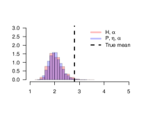
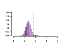
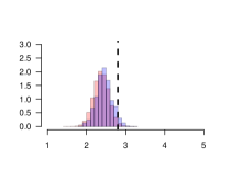
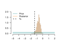
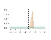
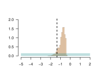
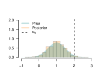
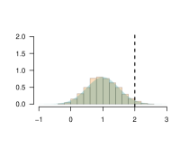
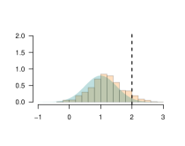
Figure 1: Posterior distributions with a prior on $\alpha$. Row 1: Histogram of draws of the posterior distribution of the functional of interest for the different parametrisations. Row 2: The prior and posterior of $\eta$. Row 3: The prior and posterior of $\alpha$.

From Figure 1 it can be seen that both methods perform similarly. When $n$ increases the variance of the posteriors decrease, but they will never converge to a Dirac measure due to the uncertainty in $\alpha$. This effect can be seen in Table 2, when compared to Table 1. The latter illustrates the identifiability of the model when $\alpha=\alpha_{0}$ is fixed. The posteriors converge to a Dirac and have proper uncertainty quantification, as the theory in this paper confirms. From Figure 1 and Table 2 it can be seen that the posteriors of the parametrisations asymptotically behave differently. The length of the credible intervals for the $P,\eta$ parametrisation are slightly smaller than those for $H$, but the coverage is higher. This means the location of this posterior is slightly different than the posterior of the functional in the other parametrisation, which is illustrated in in row 1 Figure 1. In row 3, the posterior of $\alpha$ slightly shifts compared to the prior on $\alpha$ when $n$ increases, indicating the influence of the added data. From the point of view of sensitivity analysis, the $P,\eta$ parametrisation might therefore be preferable: the credible intervals more often contains the truth when the number of observations is large. If experts don’t agree on the location of the prior on $\alpha$, but do on the direction of the relationship between $\alpha,\eta$ and $P$, the data might point the model in the right direction. When $\alpha$ is correctly specified, both parametrisations perform well and give similar results, as can be seen in the supplementary material (Eggen et al., 2023).

7 Discussion

The results in this paper justify the use of the studied Bayesian sensitivity analyses procedures in practice, with the caveat that the utility of the answers will depend on the ability of subject matter experts to express their ideas about the outcomes for those lost to follow-up through a prior on $q$. The need to incorporate expert knowledge originates from the unidentifiability of the distribution $P_{0}$ of those who dropped out and is thus not special to the Bayesian paradigm. In frequentist sensitivity analysis approaches, expert knowledge is incorporated in a variety of ways, usually through bounds on or specific values for parameters that depend on unknown, $P_{0}$-derived quantities (Liu et al., 2013). Bayesian approaches offer perhaps an advantage by allowing the user to specify their ideas about the sensitivity parameter through a probability distribution, leading to a single summary of the sensitivity analysis.

In practice, more information may be available than assumed in this paper, in the form of covariates $Z$ measured for each individual. In that case, the method can be extended to sensitivity analysis on the Missing At Random (MAR) assumption, by introducing dependence of $p,P_{1}$ and $q$ or $\eta,P$ and $q$ on $Z$. The approach taken here then becomes a Bayesian implementation of the modelling strategy proposed in Robins et al. (2000). They note that failure of the MAR assumption $Y\mathchoice{\mathrel{\hbox to0.0pt{$\displaystyle\perp$\hss}\mkern 2.0mu{\displaystyle\perp}}}{\mathrel{\hbox to0.0pt{$\textstyle\perp$\hss}\mkern 2.0mu{\textstyle\perp}}}{\mathrel{\hbox to0.0pt{$\scriptstyle\perp$\hss}\mkern 2.0mu{\scriptstyle\perp}}}{\mathrel{\hbox to0.0pt{$\scriptscriptstyle\perp$\hss}\mkern 2.0mu{\scriptscriptstyle\perp}}}R\mathchar 25194\relax Z$ is equivalent to the conditional distribution of $R\mathchar 25194\relax Z,Y$ not being free of $Y$. They then propose a sensitivity analysis by fitting a model of the type $\Pr(R=1\mathchar 25194\relax Z,Y)=\Psi\bigl{(}\eta(Z)+q(Y,Z)\bigr{)}$, for a given sensitivity function $q$, which depends on both $Y$ and $Z$. This is equivalent to (2.4) within levels of the covariate $Z$. In a Bayesian approach we need priors for this extended logistic regression model, the conditional distribution of the outcome $Y$ given $Z$, and the marginal distribution of $Z$. For a binary outcome, nonparametric priors for both conditional models can take the form of logistic Gaussian process models, as considered in Ray and van der Vaart (2020), who combine this with a Dirichlet process prior on the marginal distribution of the covariates, and prove a Bernstein-von Mises theorem under the MAR assumption. For survival outcomes, covariates could be added through a Cox proportional hazards model (Cox, 1972), for which several Bernstein-von Mises theorems exist (Kim, 2006; Kim and Lee, 2003). Another option of adding covariates is to use a dependent Dirichlet process prior (Quintana et al., 2020; MacEachern, 1999). It will be of interest to extend these results to the sensitivity setup, or from a different angle, extend the results of the present paper to include covariates.

In this paper we considered estimating a mean in the missing data problem, but this is easily extended to the estimation of an average causal effect. In the usual causal model (see Hernán and Robins (2022)), there are two potential outcomes $Y^{1}$ and $Y^{0}$, corresponding to an individual being treated $(R=1$) or not ($R=0$), and it is desired to estimate $\mathbb{E}Y^{1}-\mathbb{E}Y^{0}$, based on observing only $Y^{1}$ if $R=1$ and only $Y^{0}$ if $R=0$. In other words, one of the two potential outcomes is missing. The usual assumption, called conditional exchangeability (CE) or no unmeasured confounders, is that $Y^{r}\mathchoice{\mathrel{\hbox to0.0pt{$\displaystyle\perp$\hss}\mkern 2.0mu{\displaystyle\perp}}}{\mathrel{\hbox to0.0pt{$\textstyle\perp$\hss}\mkern 2.0mu{\textstyle\perp}}}{\mathrel{\hbox to0.0pt{$\scriptstyle\perp$\hss}\mkern 2.0mu{\scriptstyle\perp}}}{\mathrel{\hbox to0.0pt{$\scriptscriptstyle\perp$\hss}\mkern 2.0mu{\scriptscriptstyle\perp}}}R\mathchar 25194\relax Z$, for $r=0,1$, which is exactly the MAR assumption considered in the preceding paragraph. A sensitivity analysis may investigate deviations from (CE) in exactly the manner proposed.

Within the causal setting, a different modelling perspective was considered in McCandless et al. (2007, 2012), also see Gustafson et al. (2010); Gustafson and McCandless (2018); McCandless and Gustafson (2017), and Dorie et al. (2016). These authors interpret the failure of (CE) as the omission of a covariate in the conditioning. Thus they hypothesize the existence of a unmeasured confounder $U$ such that $Y^{r}\mathchoice{\mathrel{\hbox to0.0pt{$\displaystyle\perp$\hss}\mkern 2.0mu{\displaystyle\perp}}}{\mathrel{\hbox to0.0pt{$\textstyle\perp$\hss}\mkern 2.0mu{\textstyle\perp}}}{\mathrel{\hbox to0.0pt{$\scriptstyle\perp$\hss}\mkern 2.0mu{\scriptstyle\perp}}}{\mathrel{\hbox to0.0pt{$\scriptscriptstyle\perp$\hss}\mkern 2.0mu{\scriptscriptstyle\perp}}}R\mathchar 25194\relax Z,U$. Starting from a model for the distribution of $(Y^{r},R,Z,U)$, estimation of the parameter of interest is then achieved by considering this as a missing data problem with missing data $U$. Typically $U$ is assumed to be a binary variable and its effect on the other variables is modelled parametrically, although Dorie et al. (2016) allow a nonparametric relation between the outcomes and covariates $Z$.

8 Extended gamma posterior

In this section we study the posterior distribution for sampling from a prior equal to the extended gamma process. We are interested in the special case (4.1), but in this section adopt a general framework independent of the main paper. We prove a functional Bernstein-von Mises theorem and consistency of the posterior mean in the total variation norm.

For given measurable functions $b:\mathfrak{X}\to(0,\infty)$ and a finite, atomless Borel measure $a$ on the Polish space $\mathfrak{X}$, let $P_{n}$ be distributed as the normalised completely random measure without fixed atoms and continuous part with intensity measure $\nu^{c}(dx,ds)=s^{-1}e^{-sb(x)}\,ds\,da(x)$. Suppose that $P_{n}$ is used as a prior for the distribution of an i.i.d. sample of observations; hence $X_{1},\ldots,X_{n}\mathchar 25194\relax P_{n}\,\raise-2.0pt\hbox{$\stackrel{{\scriptstyle\makebox{\scriptsize iid}}}{{\sim}}$}\,P_{n}$. In this section we derive the asymptotics of the conditional distribution of $P_{n}$ given $X_{1},\ldots,X_{n}$ (i.e. the posterior distribution). In the intended application the function $b$ is equal to $b=(1+e^{\eta+q})$.

We identify probability distributions $P$ on $\mathfrak{X}$ with the stochastic processes $(Pf:f\in\mathcal{F})$, for a given collection of measurable maps $f:\mathfrak{X}\to\mathbb{R}$, and consider weak convergence of sequences of such processes in $\mathbb{R}^{\mathcal{F}}$ in the case of a finite collection, and more generally in the space $\ell^{\infty}(\mathcal{F})$ of bounded functions $z:\mathcal{F}\to\mathbb{R}$ equipped with the uniform norm $\|z\|_{\mathcal{F}}=\sup_{f\in\mathcal{F}}|z(f)|$. Weak convergence of conditional distributions is understood in terms of the bounded Lipschitz metric: we say that $Z_{n}\mathchar 25194\relax X_{n}\rightsquigarrow Z$ in probability or almost surely if $\sup_{h\in\text{BL}_{1}}\bigl{|}\mathbb{E}\bigl{(}h(Z_{n})\mathchar 25194\relax X_{n}\bigr{)}-\mathbb{E}h(Z)\bigr{|}\rightarrow 0,$ in probability or almost surely. Here $\text{BL}_{1}$ is the set of functions $h:\ell^{\infty}(\mathcal{F})\to[-1,1]$ such that $|h(z_{1})-h(z_{2})|\leq\|z_{1}-z_{2}\|_{\mathcal{F}}$, for every $z_{1},z_{2}\in\ell^{\infty}(\mathcal{F})$. Let $\mathbb{B}_{P_{0}}$ be a $P_{0}$-Brownian bridge process: a tight, Borel measurable, zero-mean Gaussian map into $\ell^{\infty}(\mathcal{F})$ with covariance function $\mathop{\rm cov}\nolimits(\mathbb{B}_{P_{0}}f,\mathbb{B}_{P_{0}}g)=P_{0}(fg)-P_{0}fP_{0}g$.

Theorem 8.1 (Bernstein-von Mises for extended gamma processes).

Let $\mathcal{F}$ be a $P_{0}$-Donsker class with measurable envelope function $F$ such that $\int F\,da<\infty$, and let $b:\mathfrak{X}\to[\underline{b},\infty)$ be a measurable function, for some constant $\underline{b}>0$. If there exist $q,r>0$ with $1/q+1/r<1/2$ such that $P_{0}b^{q}+P_{0}F^{r}<\infty$, then for $P_{0}^{\infty}$-almost every sequence $X_{1},X_{2},\ldots$,

$$\sqrt{n}\left(P_{n}-\mathbb{P}_{n}\right)\mathchar 25194\relax X_{1},\ldots,X_{n}\rightsquigarrow\mathbb{B}_{P_{0}},\qquad\text{in }\ell^{\infty}(\mathcal{F}).$$

The convergence is uniform in measurable functions $b:\mathfrak{X}\to[\underline{b},\infty)$ such that $\max_{1\leq i\leq n}\allowbreak b(X_{i})=o(n^{1/q})$ and $\mathbb{P}_{n}b-P_{0}b\rightarrow 0$, almost surely, uniformly in $b$. If the latter uniform convergence is true in probability, then the statement is true in probability, uniformly in $b$.

Proof.

Denote the distinct values in $X^{(n)}:=(X_{1},\ldots,X_{n})$ by $\tilde{X}_{1},\ldots,\tilde{X}_{K_{n}}$ and let $N_{1,n},\ldots,N_{K_{n},n}$ be their multiplicities. It was shown in James et al. (2009) (alternatively, see Theorem 14.56 of Ghosal and Van der Vaart (2017)), that the posterior distribution of $P_{n}$ is a mixture over $\lambda$ of the distributions of the normalised completely random measures $\Phi_{\lambda}/\Phi_{\lambda}(\mathfrak{X})$ with intensity measures

$$\nu^{c}_{\Phi_{\Lambda}\mathchar 25194\relax X^{(n)}}(dx,ds\mathchar 25194\relax\lambda) =s^{-1}e^{-s\bigl{(}\lambda+b(x)\bigr{)}}\,ds\,a(dx),$$ (8.1)

$$\nu^{d}_{\Phi_{\Lambda}\mathchar 25194\relax X^{(n)}}(\{\tilde{X}_{j}\},s\mathchar 25194\relax\lambda) \propto s^{N_{j,n}-1}e^{-s\bigl{(}\lambda+b(\tilde{X}_{j})\bigr{)}}\,ds,$$ (8.2)

and mixing distribution with Lebesgue density proportional to

$$\pi(\lambda\mathchar 25194\relax X^{(n)}) \propto\lambda^{n-1}e^{-\psi(\lambda)}\prod_{j=1}^{K_{n}}\frac{1}{(\lambda+b(\tilde{X}_{j}))^{N_{j,n}}},$$ (8.3)

where $\psi(\lambda):=\int\!\int_{0}^{\infty}\left(1-e^{-\lambda s}\right)s^{-1}e^{-sb(x)}\,ds\,da(x)$. For convenience of notation, let $\Lambda$ be a random variable following the mixing density (8.3), for given $X^{(n)}$. Then (see (4.3)) the posterior distribution can be interpreted as the distribution of $(P_{n}(A):A\in\mathcal{X})$ for

$$P_{n}(A)=\frac{\Psi(A)+\sum_{j=1}^{K_{n}}W_{j,K_{n}}^{\prime}\delta_{\tilde{X}_{j}}(A)}{\Psi(\mathfrak{X})+\sum_{j=1}^{K_{n}}W_{j,K_{n}}^{\prime}},$$

where the random measure $\Psi$ is distributed as $\Psi(A)=\iint\mathbbm{1}_{A}(x)s\,dN^{c}(x,s)$ conditional on $\Lambda=\lambda$, for a Poisson process $N^{c}$ on $\mathfrak{X}\times(0,\infty]$ with intensity measure (8.1), and the variables $W_{j,K_{n}}^{\prime}$ follow gamma distributions with parameters $\bigl{(}N_{j,n},\lambda+b(\tilde{X}_{j})\bigr{)}$ (as given in (8.2)), independent of each other and of $\Psi$. By the properties of the gamma distribution, for any $j\in\{1,\ldots,K_{n}\}$, we can represent $W_{j,K_{n}}^{\prime}$ as the sum of $N_{j,K_{n}}$ independent exponential random variables with intensity $\lambda+b(\tilde{X}_{j})$. This allows to simplify the preceding representation to

$$P_{n}(A)=\frac{\Psi(A)+\sum_{i=1}^{n}W_{i}\delta_{X_{i}}(A)}{\Psi(\mathfrak{X})+\sum_{i=1}^{n}W_{i}},$$ (8.4)

where conditional on $\Lambda=\lambda$ the variables $W_{1},\ldots,W_{n}$ are independent exponentially distributed with intensity parameters $\lambda+b(X_{i})$, and are independent of $\Psi$. We denote by $\mathbb{E}_{\Psi}$ and $\mathbb{E}_{W}$ the expectations with respect to $\Psi$ and the $W_{i}$, for given observations $X^{(n)}$ and given $\Lambda$. Furthermore, we denote by $\mathbb{E}_{\Lambda}$ the expectation relative to the mixture measure with density (8.3), for given $X^{(n)}$. In this notation we need to show that $\bigl{|}\mathbb{E}_{\Lambda}\mathbb{E}_{W}\mathbb{E}_{\Psi}h\bigl{(}\sqrt{n}(P_{n}-\mathbb{P}_{n})\bigr{)}-\mathbb{E}h(\mathbb{B}_{P_{0}})\bigr{|}\rightarrow 0$, almost surely (or in probability), uniformly in $h\in\text{BL}_{1}$. Define a weighted empirical distribution by $\mathbb{P}_{n}^{W}=(\sum_{i=1}^{n}W_{i}\delta_{X_{i}})/(\sum_{i=1}^{n}W_{i})$. We shall show that the following two statements are true, almost surely (or in probability), after which an application of the triangle inequality gives the desired result:

$$\sup_{h\in\text{BL}_{1}}\Bigl{|}\mathbb{E}_{\Lambda}\mathbb{E}_{W}\mathbb{E}_{\Psi}h\bigl{(}\sqrt{n}(P_{n}-\mathbb{P}_{n})\bigr{)}-\mathbb{E}_{\Lambda}\mathbb{E}_{W}h\bigl{(}\sqrt{n}(\mathbb{P}_{n}^{W}-\mathbb{P}_{n})\bigr{)}\Bigr{|}\rightarrow 0,$$ (8.5)

$$\sup_{h\in\text{BL}_{1}}\Bigl{|}\mathbb{E}_{\Lambda}\mathbb{E}_{W}h\bigl{(}\sqrt{n}(\mathbb{P}_{n}^{W}-\mathbb{P}_{n})\bigr{)}-\mathbb{E}h(\mathbb{B}_{P_{0}})\Bigr{|}\rightarrow 0.$$ (8.6)

An essential ingredient for proving these statements is that the distributions of $\Lambda$ will give probability tending to one to the sets $[cn/\log n,\infty)$, for some small $c>0$, as is shown in Lemma 8.4. This causes that the contribution of $\Psi$ to (8.4) is negligible relative to the contribution of $\mathbb{P}_{n}^{W}$, leading to (8.5). Furthermore, it causes that the $W_{i}$ will be asymptotically i.i.d. exponential variables (with large but almost equal intensities), so that the processes $\mathbb{P}_{n}^{W}$ are asymptotically equivalent to the Bayesian bootstrap process, which is known to tend to a Brownian bridge, leading to (8.6). To handle (8.5), we start by noting that, by (8.4) and the definition of $\mathbb{P}_{n}^{W}$,

$$P_{n}-\mathbb{P}_{n}^{W}=\frac{\Psi-\Psi(\mathfrak{X})\mathbb{P}_{n}^{W}}{\Psi(\mathfrak{X})+\sum_{i=1}^{n}W_{i}}.$$

Because $\|\Psi\|_{\mathcal{F}}\leq\Psi F$ and $\|\mathbb{P}_{n}^{W}\|_{\mathcal{F}}\leq M_{n}:=\max_{1\leq i\leq n}F(X_{i})$, it follows that the left side of (8.5) is bounded above by

$$\mathbb{E}_{\Lambda}\mathbb{E}_{W}\mathbb{E}_{\Psi}\bigl{\|}\sqrt{n}(P_{n}-\mathbb{P}_{n}^{W})\bigr{\|}_{\mathcal{F}}\leq\sqrt{n}\,\mathbb{E}_{\Lambda}\mathbb{E}_{W}\mathbb{E}_{\Psi}\frac{\Psi F+\Psi(\mathfrak{X})M_{n}}{\Psi(\mathfrak{X})+\sum_{i=1}^{n}W_{i}}.$$

The expression on the right side without the leading expectation on $\Lambda$ is of the form as in Lemma 8.1, with $f=F+1_{\mathfrak{X}}M_{n}$ (and with $M_{n}$ fixed due to the conditioning on $X_{1},\ldots,X_{n}$). Thus the preceding display can be bounded above by

$$\sqrt{n}\,\mathbb{E}_{\Lambda}\int_{0}^{\infty}\Bigl{[}e^{\int\log\bigl{(}(\Lambda+b)/(t+\Lambda+b)\bigr{)}\,da}\cdot\int\frac{f}{t+\Lambda+b}\,da\cdot\prod_{i=1}^{n}\frac{\Lambda+b(X_{i})}{t+\Lambda+b(X_{i})}\Bigr{]}\,dt.$$

The first term of the product in the integrand is bounded above by 1, since the logarithm in the exponent is negative. To bound the second and third terms we split the integral over $t$ in the ranges $[0,P_{0}b)$ and $[P_{0}b,\infty)$. For $t$ in the range $[0,P_{0}b)$ we use the bound $\int f/(t+\Lambda+b)\,da\leq af/(\Lambda+\underline{b})$ on the second term, where $af=\int f\,da$. Furthermore, in this range we bound the third term by 1. This shows that the integral over the range $[0,P_{0}b)$ contributes no more than $af\,P_{0}b\,\mathbb{E}_{\Lambda}\left[(\Lambda+\underline{b})^{-1}\right]$. For $t$ in the range $[P_{0}b,\infty)$, we bound the second term by $af/(t+\Lambda+\underline{b})$, while for the third term we use Jensen’s inequality on the logarithm to see that

$$\prod_{i=1}^{n}\frac{\lambda+b(X_{i})}{t+\lambda+b(X_{j})} =e^{n\int\log\big{(}\frac{\lambda+b}{t+\lambda+b}\bigr{)}\,d\mathbb{P}_{n}}\leq\Bigl{(}\mathbb{P}_{n}\frac{\lambda+b}{t+\lambda+b}\Bigr{)}^{n}\leq\Bigl{(}\frac{\lambda+\mathbb{P}_{n}b}{t+\lambda+\underline{b}}\Bigr{)}^{n}.$$

Substituting these bounds in the integral, we find

$$af\,\mathbb{E}_{\Lambda}\Bigl{[}(\Lambda+\mathbb{P}_{n}b)^{n}\int_{P_{0}b}^{\infty}\frac{1}{(t+\Lambda+\underline{b})^{n+1}}\,dt\Bigr{]} =\frac{af}{n}\mathbb{E}_{\Lambda}\Bigl{(}\frac{\Lambda+\mathbb{P}_{n}b}{P_{0}b+\Lambda+\underline{b}}\Bigr{)}^{n}.$$

Since $\underline{b}>0$ and $\mathbb{P}_{n}b-P_{0}b\rightarrow 0$, almost surely (or in probability), the quotient on the right is bounded above by 1 eventually, almost surely. Thus combining the results for the two ranges, we find that as $n\rightarrow\infty$, almost surely,

$$\mathbb{E}_{\Lambda}\mathbb{E}_{W}\mathbb{E}_{\Psi}\left[\frac{\Psi f}{\Psi(\mathfrak{X})+\sum_{i=1}^{n}W_{i}}\right]\leq af\Bigl{[}\mathbb{E}_{\Lambda}\frac{P_{0}b}{\Lambda+\underline{b}}+\frac{1}{n}\Bigr{]}$$

$$\qquad\qquad\qquad\qquad\qquad\leq af\Bigl{[}\frac{P_{0}b}{\underline{b}}\Pi\Bigl{(}\Lambda<\frac{cn}{\log n}\mathchar 25194\relax X^{(n)}\Bigr{)}+\frac{P_{0}b\,\log n}{cn}+\frac{1}{n}\Bigr{]}.$$

We substitute $f=F+1_{\mathfrak{X}}M_{n}$ in the right side and multiply by $\sqrt{n}$ to obtain a bound on (8.5) of the form

$$\bigl{(}aF+M_{n}a(\mathfrak{X})\bigr{)}\Bigl{[}\frac{P_{0}b}{\underline{b}}\sqrt{n}\,\Pi\Bigl{(}\Lambda<\frac{cn}{\log n}\mathchar 25194\relax X^{(n)}\Bigr{)}+\frac{P_{0}b\,\log n+1}{c\sqrt{n}}\Bigr{]}.$$

Here $M_{n}=O(n^{1/r})$, almost surely, for some $r>2$, by Lemma 8.2 and the assumption that $P_{0}F^{r}<\infty$. This shows that the second term tends to zero. The first term tends to zero for sufficiently small $c>0$ in view of Lemma 8.4.

We are left with showing (8.6). Given $\Lambda$ and $X^{(n)}$, the variables $\tilde{W}_{i}=W_{i}(\Lambda+b(X_{i}))/(\Lambda+\underline{b})$ are i.i.d. exponential variables with parameter $\Lambda+\underline{b}$. Since this is a scale parameter, the normalised variables $\tilde{W}_{i}/\sum_{i=1}^{n}\tilde{W}_{i}$ are equal in distribution to the normalised variables $\xi_{i}/\sum_{i=1}^{n}\xi_{i}$, for $\xi_{1},\ldots,\xi_{n}$ standard exponential variables, still conditionally on $\Lambda$ and $X^{(n)}$. This shows that the empirical process $\mathbb{P}_{n}^{\tilde{W}}$ with weights $\tilde{W}$, is equal in distribution to the Bayesian bootstrap process (see Example 3.7.9 in Van der Vaart and Wellner (2023)), conditionally given $\Lambda$, but then also unconditionally (still given $X^{(n)}$), as its distribution does not depend on $\Lambda$. By Præstgaard and Wellner (1993) (or Theorem 3.6.13 in Van der Vaart and Wellner (1996)), the Bayesian bootstrap process converges to the Brownian bridge process $\mathbb{B}_{P_{0}}$. Therefore, in view of the triangle inequality it suffices to bound the difference in (8.6) when replacing $\mathbb{P}_{n}^{W}$ by $\mathbb{P}_{n}^{\tilde{W}}$. This difference can be bounded by, with $M_{n}=\max_{1\leq i\leq n}F(X_{i})$ as before,

$$\mathbb{E}_{\Lambda}\mathbb{E}_{W}\sqrt{n}\|\mathbb{P}_{n}^{W}-\mathbb{P}_{n}^{\tilde{W}}\|_{\mathcal{F}} \leq 2M_{n}\sqrt{n}\,\mathbb{E}_{\Lambda}\mathbb{E}_{W}\frac{\sum_{i=1}^{n}|W_{i}-\tilde{W}_{i}|}{\sum_{i=1}^{n}W_{i}}$$

$$=2M_{n}\sqrt{n}\max_{1\leq i\leq n}b(X_{i})\,\mathbb{E}_{\Lambda}\left[\left(\Lambda+\underline{b}\right)^{-1}\right],$$

because $|W_{i}-\tilde{W}_{i}|=W_{i}\bigl{(}b(X_{i})-\underline{b}\bigr{)}$. We again split the expectation over $\Lambda$ in two parts to bound this by

$$2M_{n}\max_{1\leq i\leq n}b(X_{i})\Bigl{[}\frac{\sqrt{n}}{\underline{b}}\Pi\Bigl{(}\Lambda<\frac{cn}{\log n}\mathchar 25194\relax X^{(n)}\Bigr{)}+\frac{\log n}{c\sqrt{n}}\Bigr{]}.$$

Here $M_{n}=O(n^{1/r})$ and $\max_{1\leq i\leq n}b(X_{i})=O(n^{1/q})$ almost surely, by Lemma 8.2 and the integrability assumptions on $F$ and $b$, where $1/q+1/r<1/2$. it follows that the leading term is $O(n^{1/2-\epsilon})$, for some $\epsilon>0$. Together with Lemma 8.4 this shows that the expression tends to zero, for sufficiently small $c>0$. ∎

Theorem 8.2 (Posterior mean).

For $P_{0}^{\infty}$-almost every sequence $X_{1},X_{2},\ldots$,

$$\sup_{A\in\mathcal{X}}\bigl{|}\mathbb{E}\bigl{(}P_{n}(A)\mathchar 25194\relax X_{1},\ldots,X_{n}\bigr{)}-\mathbb{P}_{n}(A)\bigr{|}=O(1/n),\qquad\text{a.s.}$$

Lemma 8.1.

Let $\Psi$ be a completely random measure without fixed atoms and continuous intensity measure given by $\nu^{c}(dx,ds)=s^{-1}e^{-sb(x)}\,ds\,dx$ and let $W_{1},\ldots,W_{n}$ be independent exponential variables with means $b(X_{i})$, independent of $\Psi$. Then, for any measurable function $f:\mathfrak{X}\to[0,\infty)$,

$$\mathbb{E}_{W}\mathbb{E}_{\Psi}\left[\frac{\Psi f}{\Psi(\mathfrak{X})+\sum_{i=1}^{n}W_{i}}\right]=\int_{0}^{\infty}\Bigl{[}e^{\int\log\left(\frac{b}{t+b}\right)\,da}\cdot\int\frac{f}{t+b}\,da\cdot\prod_{i=1}^{n}\frac{b(X_{i})}{t+b(X_{i})}\Bigr{]}\,dt.$$

Lemma 8.2 (Maximum of iid random variables).

If $X_{1},\ldots,X_{n}$ are i.i.d. random variables with $\mathbb{E}|X_{i}|^{r}<\infty$ for some $r>0$, then $\max_{1\leq i\leq n}\left|X_{i}\right|n^{-1/r}\stackrel{{\scriptstyle\text{as}}}{{\longrightarrow}}0$. If $X_{1,n},\ldots,\allowbreak X_{n,n}$ are i.i.d. random variables for every $n$ such that the variables $|X_{1,n}|^{r}$ are uniformly integrable, then the assertion is true in probability.

Lemma 8.3.

For any nonnegative measurable function $b:\mathfrak{X}\to(0,\infty)$, and any $\lambda>0$, we have $\int\!\int_{0}^{\infty}(1-e^{-\lambda s})s^{-1}e^{-sb}\,ds\,da=\int\log(1+\lambda/b)\,da$.

Lemma 8.4 (Concentration of the mixing distribution).

For $\Lambda$ conditionally distributed given $X^{(n)}=(X_{1},\ldots,X_{n})$ according to density given in (8.3), for a measurable function $b:\mathfrak{X}\to[\underline{b},\infty)$ with $P_{0}b<\infty$, we have for $P_{0}^{\infty}$-almost every sequence $X_{1},X_{2},\ldots$, for any $d\in\mathbb{R}^{+}$ and $0<c<\underline{b}/\bigl{(}a(\mathfrak{X})+1+d)\bigr{)}$,

$$n^{d}\,\Pi\left(\Lambda<\frac{cn}{\log n}\mathchar 25194\relax X^{(n)}\right)\rightarrow 0.$$

The convergence is uniform in functions $b:\mathfrak{X}\to[\underline{b},\infty)$ such that the sequence $\mathbb{P}_{n}b$ remains uniformly bounded, almost surely. If the functions are uniformly bounded in probability, then the convergence is true uniformly in probability.

Correctly specified prior on $\alpha$, efficiency theory and proofs In the supplementary material, we provide additional simulation results when the prior on the sensitivity parameter is correctly specified. It also contains a derivation of the efficiency theory and some proofs not contained in the main manuscript.

References

- Balzer et al. (2020) Balzer, L. B., Ayieko, J., Kwarisiima, D., Chamie, G., Charlebois, E. D., Schwab, J., van der Laan, M. J., Kamya, M. R., Havlir, D. V., and Petersen, M. L. (2020). “Far from MCAR: Obtaining Population-level Estimates of HIV Viral Suppression.” Epidemiology, 31(5).
- Cox (1972) Cox, D. R. (1972). “Regression models and life-tables.” J. Roy. Statist. Soc. Ser. B, 34: 187–220. With discussion by F. Downton, R. Peto, D. Bartholomew, D. Lindley, P. Glassborow, D. Barton, S. Howard, B. Benjamin, J. Gart, L. Meshalkin, A. Kagan, M. Zelen, R. Barlow, J. Kalbfleisch, R. Prentice and N. Breslow, and a reply by D. R. Cox.
- Delft High Performance Computing Centre (DHPC) Delft High Performance Computing Centre (DHPC) (2022). “DelftBlue Supercomputer (Phase 1).” https://www.tudelft.nl/dhpc/ark:/44463/DelftBluePhase1.
-
Dorie et al. (2016)
Dorie, V., Harada, M., Carnegie, N. B., and Hill, J. (2016).
“A flexible, interpretable framework for assessing
sensitivity to unmeasured confounding.”
Statistics in Medicine, 35(20): 3453–3470.
URL https://onlinelibrary.wiley.com/doi/abs/10.1002/sim.6973 - Dudley (2014) Dudley, R. M. (2014). Uniform central limit theorems, volume 142 of Cambridge Studies in Advanced Mathematics. Cambridge University Press, New York, second edition.
- Eggen et al. (2023) Eggen, B., Van der Pas, S. L., and Van der Vaart, A. W. (2023). “Supplement to ”Bayesian sensitivity analysis for a missing data model”.”
-
Ferguson (1973)
Ferguson, T. S. (1973).
“A Bayesian Analysis of Some Nonparametric Problems.”
The Annals of Statistics, 1(2): 209 – 230.
URL https://doi.org/10.1214/aos/1176342360 -
Gelman et al. (1997)
Gelman, A., Gilks, W. R., and Roberts, G. O. (1997).
“Weak convergence and optimal scaling of random walk
Metropolis algorithms.”
The Annals of Applied Probability, 7(1): 110 – 120.
URL https://doi.org/10.1214/aoap/1034625254 - Ghosal and Van der Vaart (2017) Ghosal, S. and Van der Vaart, A. (2017). Fundamentals of Nonparametric Bayesian Inference. Cambridge University Press.
-
Gustafson and McCandless (2018)
Gustafson, P. and McCandless, L. C. (2018).
“When is a sensitivity parameter exactly that?”
Statist. Sci., 33(1): 86–95.
URL https://doi.org/10.1214/17-STS632 -
Gustafson et al. (2010)
Gustafson, P., McCandless, L. C., Levy, A. R., and Richardson, S. (2010).
“Simplified Bayesian sensitivity analysis for mismeasured
and unobserved confounders.”
Biometrics, 66(4): 1129–1137.
URL https://doi.org/10.1111/j.1541-0420.2009.01377.x -
Hammer et al. (1996)
Hammer, S. M., Katzenstein, D. A., Hughes, M. D., Gundacker, H., Schooley,
R. T., Haubrich, R. H., Henry, W. K., Lederman, M. M., Phair, J. P., Niu, M.,
Hirsch, M. S., and Merigan, T. C. (1996).
“A Trial Comparing Nucleoside Monotherapy with Combination
Therapy in HIV-Infected Adults with CD4 Cell Counts from 200 to 500 per Cubic
Millimeter.”
New England Journal of Medicine, 335(15): 1081–1090.
PMID: 8813038.
URL https://doi.org/10.1056/NEJM199610103351501 -
Hastings (1970)
Hastings, W. K. (1970).
“Monte Carlo Sampling Methods Using Markov Chains and Their
Applications.”
Biometrika, 57(1): 97–109.
URL http://www.jstor.org/stable/2334940 - Hernán and Robins (2022) Hernán, M. and Robins, J. (2022). “Causal Inference: What If.”
- Jacob et al. (2017) Jacob, P. E., Murray, L. M., Holmes, C. C., and Robert, C. P. (2017). “Better together? Statistical learning in models made of modules.” ArXiv:1708.08719.
-
James (2005)
James, L. (2005).
“Bayesian Poisson process partition calculus with an
application to Bayesian Lévy moving averages.”
Ann. Statist., 33(4): 1771–1799.
URL http://dx.doi.org.prox.lib.ncsu.edu/10.1214/009053605000000336 -
James et al. (2009)
James, L., Lijoi, A., and Prünster, I. (2009).
“Posterior analysis for normalized random measures with
independent increments.”
Scand. J. Stat., 36(1): 76–97.
URL http://dx.doi.org.prox.lib.ncsu.edu/10.1111/j.1467-9469.2008.00609.x -
Kim (2006)
Kim, Y. (2006).
“The Bernstein-von Mises theorem for the proportional
hazard model.”
Ann. Statist., 34(4): 1678–1700.
URL http://dx.doi.org.prox.lib.ncsu.edu/10.1214/009053606000000533 -
Kim and Lee (2003)
Kim, Y. and Lee, J. (2003).
“Bayesian bootstrap for proportional hazards models.”
Ann. Statist., 31(6): 1905–1922.
URL http://dx.doi.org.prox.lib.ncsu.edu/10.1214/aos/1074290331 - Kingman (1967) Kingman, J. (1967). “Completely random measures.” Pacific J. Math., 21: 59–78.
- Kingman (1975) — (1975). “Random discrete distribution.” J. Roy. Statist. Soc. Ser. B, 37: 1–22. With a discussion by S. J. Taylor, A. G. Hawkes, A. M. Walker, D. R. Cox, A. F. M. Smith, B. M. Hill, P. J. Burville, T. Leonard and a reply by the author.
- Little and Rubin (2019) Little, R. J. A. and Rubin, D. B. (2019). Statistical analysis with missing data. Wiley Series in Probability and Statistics. Wiley-Interscience [John Wiley & Sons], Hoboken, NJ, third edition.
- Liu et al. (2013) Liu, W., Kuramoto, S., and Stuart, E. (2013). “An introduction to sensitivity analysis for unobserved confounding in nonexperimental prevention research.” Prevention Science, 14(6): 570–580.
-
Lo (1983)
Lo, A. Y. (1983).
“Weak Convergence for Dirichlet Processes.”
Sankhyā: The Indian Journal of Statistics, Series A
(1961-2002), 45(1): 105–111.
URL http://www.jstor.org/stable/25050418 -
Lo (1986)
— (1986).
“A Remark on the Limiting Posterior Distribution of the
Multiparameter Dirichlet Process.”
Sankhyā: The Indian Journal of Statistics, Series A
(1961-2002), 48(2): 247–249.
URL http://www.jstor.org/stable/25050593 - MacEachern (1999) MacEachern, S. (1999). “Dependent nonparametric processes.” In ASA Proceedings of the Section on Bayesian Statistical Science, 50–55. American Statistical Association, pp. 50–55, Alexandria, VA.
-
McCandless and Gustafson (2017)
McCandless, L. C. and Gustafson, P. (2017).
“A comparison of Bayesian and Monte Carlo sensitivity
analysis for unmeasured confounding.”
Stat. Med., 36(18): 2887–2901.
URL https://doi.org/10.1002/sim.7298 -
McCandless et al. (2007)
McCandless, L. C., Gustafson, P., and Levy, A. (2007).