Two new algorithms for maximum likelihood estimation of sparse covariance matrices with applications to graphical modeling

Abstract

In this paper, we propose two new algorithms for maximum-likelihood estimation (MLE) of high dimensional sparse covariance matrices. Unlike most of the state-of-the-art methods, which either use regularization techniques or penalize the likelihood to impose sparsity, we solve the MLE problem based on an estimated covariance graph. More specifically, we propose a two-stage procedure: in the first stage, we determine the sparsity pattern of the target covariance matrix (in other words the marginal independence in the covariance graph under a Gaussian graphical model) using the multiple hypothesis testing method of false discovery rate (FDR), and in the second stage we use either a block coordinate descent approach to estimate the non-zero values or a proximal distance approach that penalizes the distance between the estimated covariance graph and the target covariance matrix. Doing so gives rise to two different methods, each with its own advantage: the coordinate descent approach does not require tuning of any hyper-parameters, whereas the proximal distance approach is computationally fast but requires a careful tuning of the penalty parameter. Both methods are effective even in cases where the number of observed samples is less than the dimension of the data. For performance evaluation, we test the proposed methods on both simulated and real-world data and show that they provide more accurate estimates of the sparse covariance matrix than two state-of-the-art methods.

I Introduction and Problem formulation

The estimation of covariance matrices is an extensively studied research problem in the field of multivariate analysis due to its pivotal role in a wide variety of applications such as high-dimensional classification [1], spectral analysis [2], computational biology [3], system identification [4], radar and wireless communication [5], portfolio optimization [6], asset allocation and risk assessment [7, 8, 9] and analysis of relationships between components in graphical models [10, 11].

Let $\mathbf{Y}\triangleq\left[\mathbf{y}_{1},\mathbf{y}_{2},\ldots,\mathbf{y}_{n}\right]\in\mathbb{R}^{p\times n}$ be the data matrix consisting of $n$ independent and identically distributed realizations of a $p-$variate Gaussian random variable $\mathbf{y}\in\mathbb{R}^{p}$ with zero mean and covariance matrix $\boldsymbol{\Sigma}$ $\left(\mathbf{y}\sim\mathcal{N}\left(0,\boldsymbol{\Sigma}\right)\right)$. The joint distribution of the multivariate Gaussian data $\mathbf{Y}$ is:

$$p\left(\boldsymbol{\Sigma}\right)=\left(2\pi\right)^{-\frac{pn}{2}}\left(\det\left(\boldsymbol{\Sigma}\right)\right)^{-\frac{n}{2}}\exp\left(-\frac{1}{2}\stackrel{{\scriptstyle[}}{{i}}=1]{n}{\sum}\mathbf{y}_{i}^{T}\boldsymbol{\Sigma}^{-1}\mathbf{y}_{i}\right)$$ (1)

from which the log-likelihood of the data follows:

$$\mathcal{L}\left(\boldsymbol{\Sigma}\right)=-\frac{pn}{2}\log\left(2\pi\right)-\frac{n}{2}\log\det\left(\boldsymbol{\Sigma}\right)-\frac{n}{2}\textrm{Tr}\left(\boldsymbol{\Sigma}^{-1}\mathbf{S}\right),$$ (2)

where $\mathbf{S}=\frac{1}{n}\mathbf{Y}\mathbf{Y}^{T}$ is the sample covariance matrix (SCM). To estimate $\boldsymbol{\Sigma}$ from the data $\mathbf{Y}$, the maximum likelihood estimation (MLE) problem can be cast as the minimization of the negative log-likelihood:

$$\underset{\boldsymbol{\Sigma}\succ 0}{\min}f\left(\Sigma\right)\triangleq\log\det\left(\boldsymbol{\Sigma}\right)+\textrm{Tr}\left(\boldsymbol{\Sigma}^{-1}\mathbf{S}\right)$$ (3)

When the number of samples is greater than or equal to the number of variables $\left(n\geq p\right)$, the matrix $\mathbf{S}$ is non-singular with probability one and the problem (3) has a unique solution $\hat{\boldsymbol{\Sigma}}=\mathbf{S}$. However, when $n<p$, $\mathbf{S}$ is singular. In addition, when $p$ is large, $\mathbf{S}$ is rather noisy due to the accumulation of a large number of errors. Thus, even when the sample size is greater than but comparable to the dimension of the data, $\mathbf{S}$ is a poor estimate of $\boldsymbol{\Sigma}$.

The massive data surge in recent years has led to the availability of high-dimensional data with limited sample sizes (for instance in applications such as mobile networks, social networks, and computational biology), thus making the problem of accurate covariance matrix estimation a challenging task. Therefore, any existing prior information on the covariance matrix must be exploited for its accurate estimation. Several works available in the literature exploit the intrinsic structure of the covariance matrix such as sparsity, which is a common occurrence in high-dimensional settings since many of the variables (features) are only weakly correlated and imposing sparsity in the estimation problem enables the detection of important relationships.

Motivated by the fact that in high dimensional settings many variables are weakly correlated, we formulate our problem as the estimation of a covariance matrix under the constraint that the target matrix is sparse, i.e., many of its elements are zero. Hence, the optimization problem can be written as:

$$\underset{\boldsymbol{\Sigma}\succ 0}{\min} f\left(\boldsymbol{\Sigma}\right)$$ (4)

$$\mathrm{s.t.\;} \boldsymbol{\Sigma}\in\mathcal{C}$$

where $\mathcal{C}$ is a set of sparse symmetric matrices. The assumption of sparsity is not only practical, but it also ensures that the MLE exists for cases with $n<p$.

I-A Graph motivation

The methods based on sparse covariance matrix estimation are widely used for inferring networks and graphs in high-dimensional applications. The marginal independence between random variables is encoded using a bi-directional graph where the random variables are identified by the graph vertices and two random variables are said to be marginally independent if they do not have an edge between them. Graphical models are a useful tool for discovering the structure in high-dimensional data, which is of significant interest in many applications such as social networks [12] and biology [13].

Gaussian graphical models for marginal independence, also known as Gaussian covariance graph models [14], impose sparsity on the covariance matrix. The sparsity pattern of a covariance matrix can be visualized with the help of covariance graph $\mathcal{G}\left(\mathcal{V},\mathcal{\mathcal{E}},\mathbb{I}\left(\boldsymbol{\Sigma}\right)\right)$ (notation explained at the end of this section), which has one vertex for each of the variables and a bi-directional edge between two variables if the covariance between them is non-zero. Fig. 1 shows a sparse covariance matrix and its corresponding covariance graph. The vertices $\mathcal{V}=\{1,2,3,4\}$ correspond to the indices of the random variables $\left\{y_{i}\right\}$. Two vertices $i$ and $j$ ($i\neq j$) are connected by a bidirectional edge $i\longleftrightarrow j$, if $\Sigma_{ij}$ is non-zero, i.e., $\left\{i,j\right\}\in\mathcal{E}$.

Figure 1: An example of a sparse covariance matrix with $p=4$ variables and its associated graph.

I-B Literature review

The most popular methods for sparse covariance estimation use regularized estimation techniques such as banding [15, 16], tapering [17, 18] and thresholding [19, 20, 21, 22]. In applications where the natural ordering of variables is known and the variables that are far apart are weakly correlated, methods based on banding or tapering are employed. However, these methods are sensitive to any permutation in the variables. In the absence of information on the natural ordering of variables, element-wise thresholding, which sets small entries of the SCM to zero, is useful. This is a simple and direct method to induce sparsity which is permutation-invariant with respect to indexing the variables. However, it does not guarantee a positive definite estimate. Therefore, the selection of an appropriate thresholding constant is important to balance the trade-off between positive definiteness of the estimated matrix and the desired level of sparsity. The authors of [23] and [24] resorted to the Frobenius norm approach with an $\ell_{1}$ norm penalty to enforce sparsity (soft thresholding), in which the positive definiteness of the estimate was ensured using a log-barrier term in the objective function in [23] and alternating directions methods in [24].

Similar to penalizing the Frobenius norm, the likelihood in (3) can be penalized as follows:

$$\underset{\boldsymbol{\Sigma}\succ 0}{\min}\;\log\det\left(\boldsymbol{\Sigma}\right)+\textrm{Tr}\left(\boldsymbol{\Sigma}^{-1}\mathbf{S}\right)+\lambda\left\|\mathbf{P}*\boldsymbol{\Sigma}\right\|_{1},$$ (5)

where $\lambda$ is the penalty parameter and $\mathbf{P}$ is a weight matrix (two common choices of $\mathbf{P}$ are an all-ones matrix to penalize all the elements of $\boldsymbol{\Sigma}$, and an all-ones matrix with the diagonal elements set to zero to avoid penalizing the diagonal elements of $\boldsymbol{\Sigma}$). The problem in (5) is challenging since the negative log-likelihood of the covariance matrix is not convex. The authors of [25] and [26] estimated sparse covariance matrices by solving (5) using a majorize-minimize method (SPCOV) and a coordinate descent approach, respectively. However, in general, the $\ell_{1}$ norm penalty causes shrinkage towards the origin leading to biased estimates. A better way to impose sparsity is to use the $\ell_{0}$ norm penalty in the MLE problem:

$$\underset{\boldsymbol{\Sigma}\succ 0}{\min}\;\log\det\left(\boldsymbol{\Sigma}\right)+\textrm{Tr}\left(\boldsymbol{\Sigma}^{-1}\mathbf{S}\right)+\lambda\left\|\boldsymbol{\Sigma}\right\|_{0},$$ (6)

where $\left\|\boldsymbol{\Sigma}\right\|_{0}$ denotes the number of nonzero off-diagonal elements in $\boldsymbol{\Sigma}$. However, solving (6) is even more challenging as both the negative log-likelihood and the penalty terms are non-convex. The authors of [27] replaced the $\ell_{0}$ norm in (6) with non-convex DC (difference of convex functions) approximations and solved the resultant approximate problem using DC programming techniques. Recently, the authors of [28] proposed an alternative method for solving problem (6). Specifically, they minimized the negative log-likelihood subject to the constraint that $\left\|\boldsymbol{\Sigma}\right\|_{0}\leq 2k$, where $2k$ denotes the desired number of non-zero off-diagonal elements in the covariance matrix, using a distance-to-set penalty (Euclidean distance from the target matrix to the constraint set) in place of the sparsity inducing $\ell_{0}$ norm:

$$\underset{\boldsymbol{\Sigma}}{\min}\;\log\det\left(\boldsymbol{\Sigma}\right)+\textrm{Tr}\left(\boldsymbol{\Sigma}^{-1}\mathbf{S}\right)+\frac{\rho}{2}\textrm{dist}^{2}\left(\boldsymbol{\Sigma},\mathcal{C}\right).$$ (7)

Here $\textrm{dist}^{2}\left(\boldsymbol{\Sigma},\mathcal{C}\right)$ is the minimum Euclidean distance from $\boldsymbol{\Sigma}$ to the constraint set $\mathcal{C}=\left\{\boldsymbol{\Sigma}|\boldsymbol{\Sigma}=\boldsymbol{\Sigma}^{T},\left\|\boldsymbol{\Sigma}\right\|_{0}\leq 2k\right\}$. Note that the constraint set consists of symmetric matrices with at most $2k$ non-zero off-diagonal elements but does not impose positive-definiteness. Moreover, the surrogate function used in [28] is constructed using local quadratic approximations and is not an actual upper bound on the negative log-likelihood function. Consequently, the authors of [28] had to resort to back tracking line search to ensure a monotonic decrease of the objective as well as the positive definiteness of the iterates.

Apart from imposing sparsity on the covariance matrix, a number of papers impose sparsity on the inverse covariance matrix $\boldsymbol{\Phi}\triangleq\boldsymbol{\Sigma}^{-1}$. Similar to the penalized formulation in (5), the problem of sparse inverse covariance matrix estimation is:

$$\underset{\boldsymbol{\Phi}\succ 0}{\min}\;-\log\det\left(\boldsymbol{\Phi}\right)+\textrm{Tr}\left(\boldsymbol{\Phi}\mathbf{S}\right)+\lambda\left\|\boldsymbol{\Phi}\right\|_{1}.$$ (8)

This is a convex problem whose global minimizer can be obtained using solvers like CVX [29] or iterative techniques like the graphical Lasso [30]. All the aforementioned methods [25, 26, 27, 28] including the penalized sparse inverse covariance matrix approach in (8) require the appropriate selection of tuning parameters ($\lambda$ and $k$) which is usually done via multi-fold cross-validation in which for every value of the parameter in its range the problem must be solved many times and this can become intractable for large dimensions.

Regarding the maximum likelihood estimation in covariance graphical models the published approaches include the iterative conditional fitting algorithm in [31, 32], finding gene regulatory networks in [33] and identification of multi-factor models in [34].

I-C Contributions

In this paper, we consider the problem of sparse covariance matrix estimation and propose two methods to solve it. In contrast to the state-of-the-art techniques, the proposed methods comprise two steps. In the first step, which is common to both methods, we infer the bi-directed graphical model (the underlying covariance graph) using multiple hypothesis testing, and in the second step we solve the MLE problem based on the inferred graph using two different approaches. Specifically, we determine the sparsity-pattern using the multiple hypothesis testing method of false discovery rate (FDR) applied to $\mathbf{S}$. Then in the first method, we solve the MLE problem using a block coordinate descent (BCD) approach to estimate the non-zero values. In the second method, we employ a proximal distance (PD) algorithm that uses a penalty in the ML objective to minimize the distance between the estimated graphical model and the target covariance matrix. A novelty of our framework lies in the use of hypothesis testing for estimating the sparsity of the target covariance matrix, which also involves choosing the FDR-controlling parameter. As we explain in the next section, making this choice is computationally much less complex than the cross-validation method used in other methods. The main contributions of the paper are summarized below:

1. We propose a two-step sparse covariance matrix estimation framework that infers the sparsity pattern through multiple hypothesis testing (FDR) to find the covariance graph and then solves the MLE problem using two different methods (BCD and PD) based on the estimated covariance graph.

2. The proposed BCD method can solve problem (6) which is solved via DC approximations in [27]. In addition, our PD method is a more accurate approach for solving (6) than the proximal distance algorithm in [28].

3. We test the performance of the proposed approach on both simulated data as well as real-world data (international migration data and cell signaling data) and compare the results with those corresponding to the sample covariance matrix and the state-of-the-art methods in [25] and [28].

Notations: Scalars, column vectors and matrices are denoted by italics ($a$), bold small letters ($\mathbf{a}$) and bold capital letters ($\mathbf{A}$), respectively. The $i^{\textrm{th}}$ element of a vector $\mathbf{a}$ is denoted $a_{i}$, and the $i^{\textrm{th}}$ column and $\left(i,j\right)^{\textrm{th}}$element of matrix $\mathbf{A}$ is denoted $\mathbf{a}_{i}$ and $A_{ij}$. The notations $\left(\cdot\right)^{T}$, $\left(\cdot\right)^{-1}$, $\det\left(\cdot\right)/\left|\cdot\right|$, $\textrm{Tr}\left(\cdot\right)$ and $\left\|\cdot\right\|_{F}$ are used for the transpose, inverse, determinant, trace and Frobenius norm of a matrix. $\mathbf{A}\succ 0$ denotes a positive definite matrix. $\hat{\mathbf{A}}$ denotes the estimated matrix $\mathbf{A}$, and $\mathbf{A}^{t}$ denotes the matrix $\mathbf{A}$ at the end of the $t^{\textrm{th}}$ iteration. $\mathbb{E}\left(\cdot\right)$ denotes expectation and $\mathbb{R}$ denotes the field of real numbers. $\mathcal{G}\left(\mathcal{V},\mathcal{E},\mathbf{Z}\right)$ denotes a graph where $\mathcal{V}$ is the set of vertices, $\mathcal{E}$ is the set of edges, and $\mathbf{Z}$ is the adjacency matrix. The element-wise sparsity indicator function $\mathbb{I}\left(\mathbf{X}\right)$ is defined as:

$$\mathbb{I}\left(X_{ij}\right)=\begin{cases}0&\textrm{ if }X_{ij}=0\;\textrm{must hold}\\ 1&\textrm{ otherwise }\end{cases}$$

II Proposed Methodology

The proposed sparse covariance estimation approach is a two-stage procedure. In the first stage, we use hypothesis testing to estimate the sparsity-pattern of the target covariance matrix in the form of a binary matrix $\mathbf{Z}$. Specifically we use the FDR method of multiple hypothesis testing for sparsity pattern estimation. In the second stage, we solve the MLE problem in (4) under the inferred sparsity pattern using either a BCD method or a PD method.

We first present the FDR-based hypothesis testing for inferring the covariance graph and then present the coordinate descent and proximal distance algorithms to solve the MLE problem. Lastly, we discuss the computational complexity, convergence and initialization of the proposed algorithms.

II-A First stage: Hypothesis testing

We frame the problem of detecting whether an element $\Sigma_{ij}$ of $\boldsymbol{\Sigma}$ is zero or not as a hypothesis testing problem:

$$H_{ij}:\textrm{$\Sigma_{ij}$= 0},\;i,j=1,\ldots,p,\;i\neq j$$ (9)

We will use Pearson’s correlation coefficient [35] (denoted $\rho_{ij}$) to test the null hypothesis $H_{ij}$ :

$$\rho_{ij}=\frac{S_{ij}}{\sqrt{S_{ii}S_{jj}}}$$ (10)

We compute the following test statistic:

$$T_{ij}\triangleq\rho_{ij}\sqrt{\frac{n-2}{1-\rho_{ij}^{2}}}$$ (11)

which follows a Student’s t-distribution with $n-2$ degrees of freedom under the null hypothesis [36]. In the proposed algorithms, there are a total of $M=p(p-1)/2$ hypotheses to be tested (the upper or lower triangular elements of $\boldsymbol{\Sigma}$). For ease of notation, we change the indexing of the hypotheses from using two indexes to a single index and henceforth the hypotheses are denoted as $\left\{H_{m}\right\}_{m=1}^{M}$.

II-A1 False Discovery rate (FDR)

An estimate of the sparsity pattern of $\boldsymbol{\Sigma}$ can be obtained using any testing procedure that determines which of the hypotheses in (9) should be accepted. It is in principle possible to utilize even an individual testing process that evaluates each hypothesis separately. However, because of the accumulation of the false alarm probabilities of the individual tests, such a procedure may have a high overall false alarm probability. A procedure that can test all the hypotheses simultaneously and control the total false alarm probability is therefore advised. To this end, we utilize the FDR [37, 38], which controls the expected ratio of the number of incorrectly rejected hypotheses ($IR$) to the total number of rejected hypotheses ($R$):

$$\textrm{FDR}=\mathbb{E}\left(\frac{IR}{R}\right)$$ (12)

The first step of the FDR is to rearrange the test statistics $\left\{T_{m}\right\}$ in a descending order:

$$T_{[1]}\geq T_{[2]}\geq\cdots\geq T_{[M]},$$ (13)

where $\left[\cdot\right]$ denotes the ordered indices. The significance levels used by FDR are given by [37]:

$$p_{m}=\alpha\frac{m}{M\eta_{M}},$$ (14)

where alpha is a pre-specified value that controls the desired level of FDR ($\textrm{FDR}\leq\alpha$) and $\eta_{m}$ is the harmonic number defined as $\eta_{M}=\stackrel{{\scriptstyle[}}{{i}}=1]{M}{\sum}\frac{1}{i}$ ($\approx\log M+0.577$ for large $M$). The quantiles $\left\{q_{p_{m}}\right\}$ corresponding to (14) are calculated using the Student’s t-distribution of the test statistics:

$$q_{p_{m}}:\textrm{prob}\left(T_{\left[m\right]}\geq q_{p_{m}}|H_{m}\right)=p_{m}$$ (15)

Let

$$m_{\textrm{max}}=\textrm{max}\left[m:T_{m}\geq q_{p_{m}}\right].$$ (16)

Then, we reject $H_{i}$ for $i=1,\ldots,m_{\textrm{max}}$ and accept $H_{i}$ for $i=m_{\textrm{max}}+1,\ldots,m$, or reject no hypothesis if no $m$ satisfies (16). We construct the matrix $\mathbf{Z}$, which encodes the sparsity pattern, placing zeros at the indices corresponding to the accepted hypotheses, and $1$ at the remaining indices.

II-A2 Choosing the value of $\alpha$ in FDR

We employ the model selection rule of Extended Bayesian information Criterion (EBIC) [39] to choose $\alpha$. As a first step, we grid the interval $\left[0,1\right]$ using $K$ points (say, with a spacing of $0.005$) and construct a set $\boldsymbol{\alpha}\triangleq\left\{\alpha_{k}\right\}_{k=1}^{K}$. For each $k$, we then run FDR with $\alpha_{k}$ and obtain the sparse pattern matrices $\left\{\mathbf{Z}_{k}\right\}$. Typically many values of $\alpha_{k}$’s give the same sparsity pattern. It is also important to note that the sparsity patterns obtained using FDR for increasing values of $\alpha$ are hierarchical, i.e., $\textrm{supp}\left(Z_{k-1}\right)\subseteq\textrm{supp}\left(Z_{k}\right)$ for $\alpha_{k-1}\leq\alpha_{k}$. Therefore, from the set $\boldsymbol{\alpha}$ we obtain a new set $\overline{\boldsymbol{\alpha}}$ with only those values of $\alpha_{k}$ that yield different patterns $\mathbf{Z}_{k}$. For each value of $\alpha_{k}$ in $\overline{\boldsymbol{\alpha}},$ we calculate the MLE $\hat{\boldsymbol{\Sigma}}_{k}$ of $\boldsymbol{\Sigma}$ (using the methods discussed in the next section) and the EBIC criterion:

$$\textrm{EBIC}_{k}=-2\mathcal{L}\left(\hat{\boldsymbol{\Sigma}}_{k}\right)+m_{k}\log\left(pn\right)+2m_{k}\log\left(M+p\right),$$ (17)

where $\mathcal{L}\left(\cdot\right)$ is the log-likelihood function of the multivariate Gaussian data as defined in (2) and $\small m_{k}\log\left(pn\right)+2m_{k}\log\left(M+p\right)$ is the EBIC penalty in which $m_{k}$ denotes the number of non-zero elements in $\hat{\boldsymbol{\Sigma}}_{k}$.

In Section III, we will numerically illustrate the use of FDR for choosing $\alpha$. We note here that the EBIC based choice of $\alpha$ is not as cumbersome from a computational view point as using cross-validation for choosing the penalty parameter ($\lambda$) in [25] or the sparsity level ($k$) in [28]. Firstly, the search for $\alpha$ is limited to a sub-interval of $[0,1]$ (usually $[0,0.1]$) which is not the case in the aforementioned methods where $\lambda>0$ in [25] and $0\leq k\leq$$M$ in [28]. Secondly, unlike the methods in the cited papers, in the proposed approach we need to solve the MLE problem only for a small number of values of $\alpha_{k}$ (typically less than $10$, see Fig 2 in Section III).

II-B Second stage: Solving the MLE problem

Now that we have determined a sparsity pattern of the underlying covariance matrix, we move on to estimate the non-zero $\left\{\Sigma_{ij}\right\}$ by solving the constrained problem in (4) using two different methods.

II-B1 Block Coordinate descent (BCD) method

We first present a brief overview of the general BCD method, and then discuss the proposed BCD algorithm in detail.

Block Coordinate descent

BCD is an iterative approach which can be used to solve large dimensional optimization problems of the form:

$$\underset{\mathbf{x}_{1},\mathbf{x}_{2},\ldots,\mathbf{x}_{n}}{\min} f\left(\mathbf{x}_{1},\mathbf{x}_{2},\ldots,\mathbf{x}_{n}\right)$$ (18)

$$\mathrm{s.t.\;} \mathbf{x}_{1},\mathbf{x}_{2},\ldots,\mathbf{x}_{n}\in\mathcal{X}$$

At each iteration of BCD, the problem is solved with respect to one block of the optimization variable, with the remaining blocks fixed at their values from the previous iteration. The order in which the blocks are updated can be either random or deterministic (i.e., according to some coordinate selection rule). One of the simplest deterministic way is to cyclically iterate through the variables and update them, i.e., at the $\left(t+1\right)^{\textrm{th}}$ iteration:

$$\mathbf{x}_{i}^{t+1} =\textrm{arg}\;\underset{\mathbf{x}_{i}\in\mathcal{X}}{\min}\;f\left(\mathbf{x}_{1}^{t},\mathbf{x}_{2}^{t},\ldots,\mathbf{x}_{i-1}^{t},\mathbf{x}_{i},\mathbf{x}_{i+1}^{t},\ldots,\mathbf{x}_{n}^{t}\right),$$ (19)

$$\,\,\,\,\,\,\,\,\,\,\,\,\,\,\,\,\,\,\,\,\,\,\,\,\,\,\,\,\,\,\,\,\,\,\,\,\,\,\,\,\,\,\,\,\,\,\,\,\,\,\,\,\,\,\,\,\,\,\,\,\,\,\,\,\,i=(t+1)\textrm{ mod }n$$

$$\mathbf{x}_{j}^{t+1} =\mathbf{x}_{j}^{t},\;\forall j\neq i$$ (20)

The BCD method is useful in large-scale problems where a batch update (updating all the variables together) would be too complex and computationally expensive.

The Proposed BCD method for sparse covariance matrix estimation

Let us first restate the problem (4):

$$\underset{\boldsymbol{\Sigma}\succ 0}{\min} \log\det\left(\boldsymbol{\Sigma}\right)+\textrm{Tr}\left(\boldsymbol{\Sigma}^{-1}\mathbf{S}\right)$$ (21)

$$\mathrm{s.t.\;} \boldsymbol{\Sigma}\in\mathcal{C},$$

where $\mathcal{C}\triangleq\left\{\boldsymbol{\Sigma}|\mathbb{I}\left(\boldsymbol{\Sigma}\right)=\mathbf{Z}\right\}$ is the constraint set. Problem (21) is solved using a block coordinate descent based method.

In the proposed method, we update a $2\times 2$ block of the optimization variable $\boldsymbol{\Sigma}$ at each iteration. The block to be updated is selected cyclically as follows: Let $\mathcal{V}=\left\{1,2,\ldots p\right\}$ be the set of vertices (variables), and $\mathcal{A}=\{u,v\}\subset\mathcal{V}$ be the subset that describes the block to be updated. Then, the optimization variable $\boldsymbol{\Sigma}$ at the $\left(t+1\right)^{\textrm{th}}$ iteration can be written as follows:

$$\boldsymbol{\Sigma}=\begin{bmatrix}\boldsymbol{\Sigma}_{\mathcal{AA}}&\boldsymbol{\Sigma}_{\mathcal{AB}}^{t}\\ \boldsymbol{\Sigma}_{\mathcal{BA}}^{t}&\boldsymbol{\Sigma}_{\mathcal{BB}}^{t}\end{bmatrix}$$ (22)

where $\mathcal{AA}=\mathcal{A}\times\mathcal{A}$ gives the indices of the block to be updated at $\left(t+1\right)^{\textrm{th}}$ iteration and $\mathcal{AB}=\mathcal{A}\times\mathcal{B}$, $\mathcal{BA}=\mathcal{B}\times\mathcal{A}$ and $\mathcal{BB}=\mathcal{B}\times\mathcal{B}$ give the indices of the updated blocks from the previous $t^{\textrm{th}}$ iteration. It is worth mentioning that the block $\boldsymbol{\Sigma}_{\mathcal{AA}}$ to be updated can lie anywhere in the matrix $\boldsymbol{\Sigma}$. However for the ease of derivation and notation, we move it to the top-left corner using a permutation matrix $\mathbf{U}$. The matrix $\mathbf{U}$ is constructed by interchanging the $u^{\textrm{th}}$ and $v^{\textrm{th}}$ column of an identity matrix with its first and second columns, respectively. Then, the optimization variable $\boldsymbol{\Sigma}$ as well as the matrices $\mathbf{S}$ and $\mathbf{Z}$ are pre-multiplied with $\mathbf{U}^{T}$ and post-multiplied with $\mathbf{U}$ for rearrangement of the elements.

Thus, the problem to be solved at the $\left(t+1\right)^{\textrm{th}}$ iteration can be written as:

$$\underset{\boldsymbol{\Sigma}_{AA}\succ 0}{\min} \textrm{Tr}\left(\begin{bmatrix}\boldsymbol{\Sigma}_{\mathcal{AA}}&\boldsymbol{\Sigma}_{\mathcal{AB}}^{t}\\ \boldsymbol{\Sigma}_{\mathcal{BA}}^{t}&\boldsymbol{\Sigma}_{\mathcal{BB}}^{t}\end{bmatrix}^{-1}\begin{bmatrix}\mathbf{S}_{\mathcal{AA}}&\mathbf{S}_{\mathcal{AB}}\\ \mathbf{S}_{\mathcal{BA}}&\mathbf{S}_{\mathcal{BB}}\end{bmatrix}\right)$$ (23)

$$+\log\begin{vmatrix}\boldsymbol{\Sigma}_{\mathcal{AA}}&\boldsymbol{\Sigma}_{\mathcal{AB}}^{t}\\ \boldsymbol{\Sigma}_{\mathcal{BA}}^{t}&\boldsymbol{\Sigma}_{\mathcal{BB}}^{t}\end{vmatrix}$$

$$\mathrm{s.t.\;} \mathbb{I}\left(\boldsymbol{\Sigma}_{\mathcal{AA}}\right)=\mathbf{Z}_{\mathcal{AA}},$$

where $\mathbf{Z}_{\mathcal{AA}}\in[0,1]^{2\times 2}$ is the upper left block of the matrix $\mathbf{Z}$. Next, we express $\left|\boldsymbol{\Sigma}\right|$ in terms of the variable $\boldsymbol{\Sigma}_{AA}$ as shown below:

$$\left|\boldsymbol{\Sigma}\right| =\begin{vmatrix}\mathbf{I}&\boldsymbol{\Sigma}_{\mathcal{AB}}^{t}\\ \mathbf{0}&\boldsymbol{\Sigma}_{\mathcal{BB}}^{t}\end{vmatrix}\begin{vmatrix}\boldsymbol{\Sigma}_{\mathcal{AA}}-\boldsymbol{\Sigma}_{\mathcal{AB}}^{t}\left(\boldsymbol{\Sigma}_{\mathcal{BB}}^{t}\right)^{-1}\boldsymbol{\Sigma}_{\mathcal{BA}}^{t}&\mathbf{0}\\ \left(\boldsymbol{\Sigma}_{\mathcal{BB}}^{t}\right)^{-1}\boldsymbol{\Sigma}_{\mathcal{BA}}^{t}&\mathbf{I}\end{vmatrix}$$ (24)

$$=\left|\boldsymbol{\Sigma}_{\mathcal{BB}}^{t}\right|\left|\boldsymbol{\Sigma}_{\mathcal{AA}}-\boldsymbol{\Sigma}_{\mathcal{AB}}^{t}\left(\boldsymbol{\Sigma}_{\mathcal{BB}}^{t}\right)^{-1}\boldsymbol{\Sigma}_{\mathcal{BA}}^{t}\right|$$

$$=\left|\boldsymbol{\Sigma}_{\mathcal{BB}}^{t}\right|\left|\boldsymbol{\Sigma}_{\mathcal{AA}}-\boldsymbol{\Psi}\right|$$

$$=\left|\boldsymbol{\Sigma}_{\mathcal{BB}}^{t}\right|\left|\bar{\boldsymbol{\Sigma}}\right|$$

where $\boldsymbol{\Psi}\triangleq\boldsymbol{\Sigma}_{\mathcal{AB}}^{t}\left(\boldsymbol{\Sigma}_{\mathcal{BB}}^{t}\right)^{-1}\boldsymbol{\Sigma}_{\mathcal{BA}}^{t}$ and $\bar{\boldsymbol{\Sigma}}\triangleq\boldsymbol{\Sigma}_{\mathcal{AA}}-\boldsymbol{\Psi}$. Similarly,

$$\boldsymbol{\Sigma}^{-1} =\begin{bmatrix}\bar{\boldsymbol{\Sigma}}&\mathbf{0}\\ \left(\boldsymbol{\Sigma}_{\mathcal{BB}}^{t}\right)^{-1}\boldsymbol{\Sigma}_{\mathcal{BA}}^{t}&\mathbf{I}\end{bmatrix}^{-1}\begin{bmatrix}\mathbf{I}&\boldsymbol{\Sigma}_{\mathcal{AB}}^{t}\\ \mathbf{0}&\boldsymbol{\Sigma}_{\mathcal{BB}}^{t}\end{bmatrix}^{-1}$$ (25)

$$=\begin{bmatrix}\bar{\boldsymbol{\Sigma}}^{-1}&\mathbf{0}\\ -\left(\boldsymbol{\Sigma}_{\mathcal{BB}}^{t}\right)^{-1}\boldsymbol{\Sigma}_{\mathcal{BA}}^{t}\bar{\boldsymbol{\Sigma}}^{-1}&\mathbf{I}\end{bmatrix}\begin{bmatrix}\mathbf{I}&-\boldsymbol{\Sigma}_{\mathcal{AB}}^{t}\left(\boldsymbol{\Sigma}_{\mathcal{BB}}^{t}\right)^{-1}\\ \mathbf{0}&\left(\boldsymbol{\Sigma}_{\mathcal{BB}}^{t}\right)^{-1}\end{bmatrix}$$

$$=\small\begin{bmatrix}\bar{\boldsymbol{\Sigma}}^{-1}&-\bar{\boldsymbol{\Sigma}}^{-1}\boldsymbol{\Sigma}_{\mathcal{AB}}^{t}\left(\boldsymbol{\Sigma}_{\mathcal{BB}}^{t}\right)^{-1}\\ -\left(\boldsymbol{\Sigma}_{\mathcal{BB}}^{t}\right)^{-1}\boldsymbol{\Sigma}_{\mathcal{BA}}^{t}\bar{\boldsymbol{\Sigma}}^{-1}&\left(\left(\boldsymbol{\Sigma}_{\mathcal{BB}}^{t}\right)^{-1}\boldsymbol{\Sigma}_{\mathcal{BA}}^{t}\bar{\boldsymbol{\Sigma}}^{-1}\boldsymbol{\Sigma}_{\mathcal{AB}}^{t}\right.\\ &\left.\left(\boldsymbol{\Sigma}_{\mathcal{BB}}^{t}\right)^{-1}+\left(\boldsymbol{\Sigma}_{\mathcal{BB}}^{t}\right)^{-1}\right)\end{bmatrix}$$

$$=\begin{bmatrix}\bar{\boldsymbol{\Sigma}}^{-1}&-\bar{\boldsymbol{\Sigma}}^{-1}\boldsymbol{\Phi}^{T}\\ -\boldsymbol{\Phi}\bar{\boldsymbol{\Sigma}}^{-1}&\boldsymbol{\Phi}\bar{\boldsymbol{\Sigma}}^{-1}\boldsymbol{\Phi}^{T}+\left(\boldsymbol{\Sigma}_{\mathcal{BB}}^{t}\right)^{-1}\end{bmatrix},$$

where $\boldsymbol{\Phi}\triangleq\left(\boldsymbol{\Sigma}_{\mathcal{BB}}^{t}\right)^{-1}\boldsymbol{\Sigma}_{\mathcal{BA}}^{t}$. Using (24) and (25) in (23), and ignoring the constants, we get:

$$\underset{\bar{\boldsymbol{\Sigma}}\succ 0}{\min} \textrm{Tr}\left(\begin{bmatrix}\bar{\boldsymbol{\Sigma}}^{-1}&-\bar{\boldsymbol{\Sigma}}^{-1}\boldsymbol{\Phi}^{T}\\ -\boldsymbol{\Phi}\bar{\boldsymbol{\Sigma}}^{-1}&\boldsymbol{\Phi}\bar{\boldsymbol{\Sigma}}^{-1}\boldsymbol{\Phi}^{T}+\left(\boldsymbol{\Sigma}_{\mathcal{BB}}^{t}\right)^{-1}\end{bmatrix}\mathbf{S}\right)+\log\left|\bar{\boldsymbol{\Sigma}}\right|$$ (26)

$$\mathrm{s.t.\;} \mathbb{I}\left(\bar{\boldsymbol{\Sigma}}+\boldsymbol{\Psi}\right)=\mathbf{Z}_{\mathcal{AA}}$$

which can be compactly written as:

$$\underset{\bar{\boldsymbol{\Sigma}}\succ 0}{{\rm min}} g\left(\bar{\boldsymbol{\Sigma}}\right)\triangleq\mathrm{Tr}\left(\boldsymbol{\Theta}\bar{\boldsymbol{\Sigma}}^{-1}\right)+\mathrm{log}\left|\bar{\boldsymbol{\Sigma}}\right|$$ (27)

$$\mathrm{s.t.\;} \mathbb{I}\left(\bar{\boldsymbol{\Sigma}}+\boldsymbol{\Psi}\right)=\mathbf{Z}_{\mathcal{AA}}$$

where $\boldsymbol{\Theta}\triangleq\mathbf{S}_{\mathcal{AA}}-\mathbf{S}_{\mathcal{AB}}\boldsymbol{\Phi}-\boldsymbol{\Phi}^{T}\mathbf{S}_{\mathcal{BA}}+\boldsymbol{\Phi}^{T}\mathbf{S}_{\mathcal{BB}}\boldsymbol{\Phi}$. Since $\boldsymbol{\Theta}$ is positive-definite, $g\left(\bar{\boldsymbol{\Sigma}}\right)$ is bounded from below. Moreover $g\left(\bar{\boldsymbol{\Sigma}}\right)$ is convex in $\bar{\boldsymbol{\Sigma}}^{-1}$ and therefore has a unique minimum $\hat{\bar{\boldsymbol{\Sigma}}}=\boldsymbol{\Theta}$ (and $\hat{\boldsymbol{\Sigma}}_{\mathcal{AA}}=\boldsymbol{\Theta}+\boldsymbol{\Psi}$), which will also be the solution of the constrained problem (27) if the constraint $\mathbb{I}\left(\boldsymbol{\Theta}+\boldsymbol{\Psi}\right)=\mathbf{Z}_{\mathcal{AA}}$ is satisfied. To solve the constrained problem (27) we proceed as follows.

If $\left(\mathbf{Z}_{\mathcal{AA}}\right)_{12}=1$, then the element $\bar{\boldsymbol{\Sigma}}_{12}+\boldsymbol{\Psi}_{12}$ may or may not be zero, i.e., there is no restriction on the solution and the block $\boldsymbol{\mathbf{\Sigma}}_{\mathcal{AA}}$ is updated as $\boldsymbol{\Sigma}_{\mathcal{AA}}^{t+1}=\boldsymbol{\Theta}+\boldsymbol{\Psi}$. However, if $\left(\mathbf{Z}_{\mathcal{AA}}\right)_{12}=0$, then to satisfy the constraint the optimal solution is (note that $\bar{\boldsymbol{\Sigma}}$ and $\boldsymbol{\Psi}$ are $2\times 2$ matrices):

$$\hat{\bar{\Sigma}}_{12}=-\Psi_{12}$$ (28)

To find the optimal values of $\bar{\Sigma}_{11}$ and $\bar{\Sigma}_{22}$ in this case, we rewrite equation (27) using $\bar{\Sigma}_{12}=-\Psi_{12}$ to get:

$$\underset{\bar{\boldsymbol{\Sigma}}\succ 0}{{\rm min}} \mathrm{Tr}\left(\begin{bmatrix}\Theta_{11}&\Theta_{12}\\ \Theta_{12}&\Theta_{22}\end{bmatrix}\begin{bmatrix}\bar{\Sigma}_{11}&-\Psi_{12}\\ -\Psi_{12}&\bar{\Sigma}_{22}\end{bmatrix}^{-1}\right)$$ (29)

$$+\mathrm{log}\begin{vmatrix}\bar{\Sigma}_{11}&-\Psi_{12}\\ -\Psi_{12}&\bar{\Sigma}_{22}\end{vmatrix}$$

or equivalently

$$\underset{\bar{\boldsymbol{\Sigma}}\succ 0}{{\rm min}} \frac{1}{\bar{\Sigma}_{11}\bar{\Sigma}_{22}-\Psi_{12}^{2}}\left(\Theta_{11}\bar{\Sigma}_{22}+2\Theta_{12}\Psi_{12}+\Theta_{22}\bar{\Sigma}_{11}\right)$$ (30)

$$+\mathrm{log}\left(\bar{\Sigma}_{11}\bar{\Sigma}_{22}-\Psi_{12}^{2}\right)$$

Note that the constraint $\bar{\boldsymbol{\Sigma}}\succ 0$ in (29) is a convex set and the cost function in (29) is bounded from below over the set. Additionally, on the boundary of this set the objective function in (29) tends to $+\infty$. Therefore, the problem in (29) has a bounded global minimum.

Differentiating (30) with respect to $\bar{\Sigma}_{11}$ gives:

$$\Theta_{22}+\bar{\Sigma}_{22}=\frac{\left(\Theta_{11}\bar{\Sigma}_{22}+2\Theta_{12}\Psi_{12}+\Theta_{22}\bar{\Sigma}_{11}\right)\bar{\Sigma}_{22}}{\left(\bar{\Sigma}_{11}\bar{\Sigma}_{22}-\Psi_{12}^{2}\right)}$$ (31)

Similarly, differentiating (30) with respect to $\bar{\Sigma}_{22}$ gives:

$$\Theta_{11}+\bar{\Sigma}_{11}=\frac{\left(\Theta_{11}\bar{\Sigma}_{22}+2\Theta_{12}\Psi_{12}+\Theta_{22}\bar{\Sigma}_{11}\right)\bar{\Sigma}_{11}}{\left(\bar{\Sigma}_{11}\bar{\Sigma}_{22}-\Psi_{12}^{2}\right)}$$ (32)

Dividing (31) by (32) yields:

$$\bar{\Sigma}_{22}=\frac{\Theta_{22}}{\Theta_{11}}\bar{\Sigma}_{11}$$ (33)

Substituting for $\bar{\Sigma}_{22}$ in (31) we have that:

$$\Theta_{22}\bar{\Sigma}_{11}^{3}-\Theta_{22}\Theta_{11}\bar{\Sigma}_{11}^{2}-\Theta_{11}(\Psi_{12}^{2}+2\Theta_{12}\Psi_{12})\bar{\Sigma}_{11}-\Psi_{12}^{2}\Theta_{11}^{2}=0$$ (34)

which is a cubic equation in $\bar{\Sigma}_{11}$. Note that the first coefficient ($\Theta_{22}$) is positive, and the second and the fourth coefficients ($-\Theta_{22}\Theta_{11}$ and $-\Psi_{12}^{2}\Theta_{11}^{2}$) are negative (since $\Theta_{11}$ and $\Theta_{22}$ are positive quantities), therefore, depending on the sign of the third coefficient $-\Theta_{11}(\Psi_{12}^{2}+2\Theta_{12}\Psi_{12})$, (34) can have either one or three positive solutions. If $\Psi_{12}^{2}+2\Theta_{12}\Psi_{12}$ is positive, then by Descartes’ rule of signs, there is exactly one positive solution of (34) which gives the optimal value $\bar{\Sigma}_{11}.$ However, if $\Psi_{12}^{2}+2\Theta_{12}\Psi_{12}$ is negative, then there might be three positive solutions of which the one that yields the lowest value of the objective in (27) gives the optimal value of $\bar{\Sigma}_{11}.$ Thus, in the present case, the block $\mathbf{\Sigma}_{\mathcal{AA}}$ is updated as:

$$\mathbf{\boldsymbol{\Sigma}}_{\mathcal{AA}}^{t+1}=\begin{bmatrix}\hat{\bar{\Sigma}}_{11}+\Psi_{11}&0\\ 0&\hat{\bar{\Sigma}}_{22}+\Psi_{22}\end{bmatrix}$$ (35)

The stationary point of (29) thus obtained via the aforementioned method is also the global minimizer. This proves that the covariance matrix $\bar{\boldsymbol{\Sigma}}^{t+1}$ obtained at the end of each iteration is positive definite. The matrix $\mathbf{\boldsymbol{\Sigma}}_{\mathcal{AA}}^{t+1}$ at each iteration is also positive definite because when $\left(\mathbf{Z}_{\mathcal{AA}}\right)_{12}=1$, $\mathbf{\boldsymbol{\Sigma}}_{\mathcal{AA}}^{t+1}$ is equal to the sum of two positive definite matrices $\boldsymbol{\Theta}$ and $\boldsymbol{\Psi}$, and when $\left(\mathbf{Z}_{\mathcal{AA}}\right)_{12}=0$, $\mathbf{\boldsymbol{\Sigma}}_{\mathcal{AA}}^{t+1}$ is a diagonal matrix with positive elements $\hat{\bar{\Sigma}}_{11}+\Psi_{11}$ and $\hat{\bar{\Sigma}}_{22}+\Psi_{22}$ on the diagonal. Since both $\mathbf{\boldsymbol{\Sigma}}_{\mathcal{AA}}^{t+1}$ and $\bar{\boldsymbol{\Sigma}}^{t+1}$ (which is the Schur complement of $\mathbf{\boldsymbol{\Sigma}}_{\mathcal{AA}}^{t+1}$) are positive definite, the matrix $\mathbf{\boldsymbol{\Sigma}}^{t+1}$ as defined in (22) is also positive definite. We would also like to note that when $\left(\mathbf{Z}_{\mathcal{AA}}\right)_{12}=1$, the algorithm may introduce zeros in the estimated covariance matrix in addition to those in the initial sparsity pattern constraint.

Algorithm 1 The BCD algorithm

Input: $\mathbf{S}$, $\alpha$ , $\epsilon$

Initialize: $t=0$, $\mathbf{\boldsymbol{\Sigma}}^{0}$

• Determine the sparsity pattern matrix $\mathbf{Z}$ using FDR as discussed in Section II-A.

Iterate

for $u=1:p-1$

for

$v=u+1:p$

• Compute $\mathbf{U}$ and rearrange the matrices $\boldsymbol{\Sigma}$, $\mathbf{Z}$ and $\mathbf{S}$ using the permutation matrix $\mathbf{U}$.

• Compute $\boldsymbol{\Theta}$ and $\boldsymbol{\Psi}$.

• If $\left(Z_{\mathcal{AA}}\right)_{12}=1$, then:

  • $\mathbf{\boldsymbol{\Sigma}}_{\mathcal{AA}}^{t+1}=\boldsymbol{\Theta}+\boldsymbol{\Psi}$

  Else

  • $\hat{\bar{\Sigma}}_{12}=-\Psi_{12}$

  • Solve (34) and (33) to obtain $\hat{\bar{\Sigma}}_{11}$ and $\hat{\bar{\Sigma}}_{22}$.

  • $\mathbf{\boldsymbol{\Sigma}}_{\mathcal{AA}}^{t+1}=\hat{\bar{\boldsymbol{\Sigma}}}+\boldsymbol{\Psi}$

• $\boldsymbol{\Sigma}^{t+1}=\mathbf{U}\begin{bmatrix}\boldsymbol{\Sigma}_{\mathcal{AA}}^{t+1}&\boldsymbol{\Sigma}_{\mathcal{AB}}^{t}\\ \boldsymbol{\Sigma}_{\mathcal{BA}}^{t}&\boldsymbol{\Sigma}_{\mathcal{BB}}^{t}\end{bmatrix}\mathbf{U}^{T}$

end

end

• $t=t+1$

Stop and return $\boldsymbol{\Sigma}^{t+1}$ if $\left\|\boldsymbol{\Sigma}^{t+1}-\boldsymbol{\Sigma}^{t}\right\|_{F}/\left\|\boldsymbol{\Sigma}^{t}\right\|_{F}<\epsilon$

Output: $\hat{\boldsymbol{\Sigma}}=\boldsymbol{\Sigma}^{t+1}$ at convergence.

Algorithm 1 summarizes the pseudo-code of the BCD algorithm.

Remark 1.

It is worth mentioning that the proposed method BCD can be used to solve the $\ell_{0}$ norm regularized problem (6) after a slight modification. The $2\times 2$ problem in (27) can be written with the $\ell_{0}$ norm penalty as:

$$\begin{aligned} \underset{\bar{\boldsymbol{\Sigma}}\succ 0}{{\rm min}}\>&\mathrm{Tr}\left(\boldsymbol{\Theta}\bar{\boldsymbol{\Sigma}}^{-1}\right)+\mathrm{log}\left|\bar{\boldsymbol{\Sigma}}\right|+\lambda\left\|\bar{\boldsymbol{\Sigma}}+\boldsymbol{\Psi}\right\|_{0}\end{aligned},$$ (36)

for which two possible solutions exists: either the off-diagonal elements of $\boldsymbol{\Sigma}_{\mathcal{AA}}=\bar{\boldsymbol{\Sigma}}+\boldsymbol{\Psi}$ are zero and thus $\bar{\Sigma}_{12}^{*}=\bar{\Sigma}_{21}^{*}=-\Psi_{12}$ and $\bar{\Sigma}_{11}^{*}$, $\bar{\Sigma}_{22}^{*}$ can be obtained from (33) and (34), or the off-diagonal elements of $\boldsymbol{\Sigma}_{\mathcal{AA}}$ are non-zero in which case (36) has the closed-form solution $\bar{\boldsymbol{\Sigma}}^{*}=\boldsymbol{\Theta}$. The solution that yields the lower value of the objective function in (3) is chosen as the optimal solution.

II-B2 Proximal distance approach

In this sub-section we first introduce the general proximal distance algorithm, and then discuss the proposed PD method in detail.

Proximal distance algorithm

This type of algorithm is a combination of the classical Courant’s penalty method of constrained optimization and the principle of majorization-minimization (MM). Consider a constrained optimization problem of the form:

$$\underset{\mathbf{x}\in\mathcal{C}}{\textrm{min}}\;f\left(\mathbf{x}\right),$$ (37)

where $\mathcal{C}$ is the constraint set. Using the mentioned penalty method the constrained problem (37) can be written as an unconstrained problem as follows:

$$\underset{\mathbf{x}}{\textrm{min}}\;f\left(\mathbf{x}\right)+\rho q\left(\mathbf{x}\right)$$ (38)

where the penalty $q\left(\mathbf{x}\right)$ is nonnegative and equal to zero when $\mathbf{x}\in\mathcal{C}$. For $q\left(\mathbf{x}\right)\triangleq\frac{1}{2}\textrm{dist}^{2}\left(\mathbf{x},\mathcal{C}\right)$, (38) can be written as:

$$\underset{\mathbf{x}}{\textrm{min}}\;f\left(\mathbf{x}\right)+\frac{\rho}{2}\textrm{dist}^{2}\left(\mathbf{x},\mathcal{C}\right).$$ (39)

Using the Euclidean distance in (39) we get:

$$\underset{\mathbf{x}}{\textrm{min}}\;f\left(\mathbf{x}\right)+\frac{\rho}{2}\left\|\mathbf{x}-P_{\mathcal{C}}\left(\mathbf{x}\right)\right\|^{2},$$ (40)

where $P_{\mathcal{C}}\left(\mathbf{x}\right)$ is the orthogonal projection of $\mathbf{x}$ on $\mathcal{C}$ that minimizes the norm. In the next step, the quadratic penalty is majorized using MM. Before describing that step, we review the MM principle.

Let $h\left(\mathbf{x}\right)$ be the function to be minimized. In the first step of MM, for a given $\mathbf{x}^{t}$ a surrogate $g\left(\mathbf{x}|\mathbf{x}^{t}\right)$ that has the following properties is constructed:

$$g\left(\mathbf{x}|\mathbf{x}^{t}\right) \geq h\left(\mathbf{x}\right)\;\textrm{and }$$ (41)

$$g\left(\mathbf{x}^{t}|\mathbf{x}^{t}\right) =h\left(\mathbf{x}^{t}\right)$$ (42)

In the second step, the surrogate is minimized to obtain the next update:

$$\mathbf{x}^{t+1}=\underset{\mathbf{x}}{\textrm{argmin }}g\left(\mathbf{x}|\mathbf{x}^{t}\right)$$ (43)

From (41), (42), and (43), one can verify that:

$$h\left(\mathbf{x}^{t+1}\right)\leq g\left(\mathbf{x}^{t+1}|\mathbf{x}^{t}\right)\leq g\left(\mathbf{x}^{t}|\mathbf{x}^{t}\right)=h\left(\mathbf{x}^{t}\right).$$ (44)

Therefore an MM algorithm monotonically decreases the objective function. The key ingredient of such an algorithm is the construction of the surrogate, which should closely follow the objective function and should be simple to minimize. For details on the construction of surrogate functions, we refer to [40].

Using the MM principle, a surrogate for the problem (40) is constructed majorizing the distance term:

$$g\left(\mathbf{x}|\mathbf{x}^{t}\right)\triangleq f\left(\mathbf{x}\right)+\frac{\rho}{2}\left\|\mathbf{x}-P_{\mathcal{C}}\left(\mathbf{x}^{t}\right)\right\|^{2},$$ (45)

For more details on proximal distance algorithms, the interested readers can consult [41].

The Proposed PD method for sparse covariance matrix estimation

The problem of sparse covariance matrix estimation with distance penalty can be written as:

$$\underset{\boldsymbol{\Sigma}\succ 0}{\textrm{min}}\log\left|\boldsymbol{\Sigma}\right|+\textrm{Tr}\left(\mathbf{\boldsymbol{\Sigma}}^{-1}\mathbf{S}\right)+\frac{\rho}{2}\textrm{dist}^{2}\left(\boldsymbol{\Sigma},\mathcal{C}\right)$$ (46)

where $\textrm{dist}^{2}\left(\mathbf{\boldsymbol{\Sigma}},\mathcal{C}\right)$ is the squared distance from $\mathbf{\boldsymbol{\Sigma}}$ to $\mathcal{C}$ and $\rho$ is the penalty parameter. Writing the distance penalty term using the Frobenius norm, we get:

$$\begin{aligned} \underset{\boldsymbol{\Sigma}\succ 0}{\textrm{min}}&\log\left|\boldsymbol{\Sigma}\right|+\textrm{Tr}\left(\boldsymbol{\Sigma}^{-1}\mathbf{S}\right)+\frac{\rho}{2}\left\|\boldsymbol{\Sigma}-P_{\mathcal{C}}\left(\boldsymbol{\Sigma}\right)\right\|_{F}^{2}\end{aligned},$$ (47)

Problem (47) can also be written as:

$$\underset{\boldsymbol{\Sigma}\succ 0}{\textrm{min}} \textrm{Tr}\left[\boldsymbol{\Sigma}^{-1}\left(\mathbf{S}-\nu\mathbf{I}\right)\right]+\textrm{Tr}\left(\nu\boldsymbol{\Sigma}^{-1}\right)+\log\left|\boldsymbol{\Sigma}\right|$$ (48)

$$+\frac{\rho}{2}\left\|\boldsymbol{\Sigma}-P_{\mathcal{C}}\left(\boldsymbol{\Sigma}\right)\right\|_{F}^{2},$$

where

$$\nu=\lambda_{\textrm{max}}\left(\mathbf{S}\right)$$ (49)

Majorizing the distance penalty as in (45) and the concave terms $\log\left|\boldsymbol{\Sigma}\right|$ and $\textrm{Tr}\left(\mathbf{\boldsymbol{\Sigma}}^{-1}\left(\mathbf{S}-\nu\mathbf{I}\right)\right)$ using their tangent hyperplanes, we get the following surrogate problem:

$$\underset{\boldsymbol{\Sigma}\succ 0}{\textrm{min}} -\textrm{Tr}\left[\left(\boldsymbol{\Sigma}^{t}\right)^{-1}\left(\mathbf{S}-\nu\mathbf{I}\right)\left(\boldsymbol{\Sigma}^{t}\right)^{-1}\boldsymbol{\Sigma}\right]+\textrm{Tr}\left(\left(\boldsymbol{\Sigma}^{t}\right)^{-1}\boldsymbol{\Sigma}\right)$$ (50)

$$+\textrm{Tr}\left(\nu\mathbf{\boldsymbol{\Sigma}}^{-1}\right)+\frac{\rho}{2}\left\|\boldsymbol{\Sigma}-P_{\mathcal{C}}\left(\boldsymbol{\Sigma}^{t}\right)\right\|_{F}^{2}$$

Expanding the distance penalty term and ignoring the constants yields the following problem:

$$\underset{\boldsymbol{\Sigma}\succ 0}{\textrm{min}} \textrm{Tr}\left[\left(\left(\boldsymbol{\Sigma}^{t}\right)^{-1}-\left(\boldsymbol{\Sigma}^{t}\right)^{-1}\left(\mathbf{S}-\nu\mathbf{I}\right)\left(\boldsymbol{\Sigma}^{t}\right)^{-1}\right)\boldsymbol{\Sigma}\right]$$ (51)

$$+\textrm{Tr}\left(\nu\mathbf{\boldsymbol{\Sigma}}^{-1}\right)-\rho\textrm{Tr}\left[\boldsymbol{\Sigma}P_{\mathcal{C}}\left(\boldsymbol{\Sigma}^{t}\right)\right]+\frac{\rho}{2}\left\|\boldsymbol{\Sigma}\right\|_{F}^{2}$$

which can be rewritten as:

$$\underset{\boldsymbol{\Sigma}\succ 0}{\textrm{min}} \textrm{Tr}\left\{\left[\left(\boldsymbol{\Sigma}^{t}\right)^{-1}-\left(\boldsymbol{\Sigma}^{t}\right)^{-1}\left(\mathbf{S}-\nu\mathbf{I}\right)\left(\boldsymbol{\Sigma}^{t}\right)^{-1}\right.\right.$$ (52)

$$\left.\left.-\rho P_{\mathcal{C}}\left(\boldsymbol{\Sigma}^{t}\right)\right]\mathbf{\boldsymbol{\Sigma}}\right\}+\textrm{Tr}\left(\nu\boldsymbol{\Sigma}^{-1}\right)+\frac{\rho}{2}\left\|\boldsymbol{\Sigma}\right\|_{F}^{2}$$

Let

$$\mathbf{A}\triangleq\left(\boldsymbol{\Sigma}^{t}\right)^{-1}-\left(\boldsymbol{\Sigma}^{t}\right)^{-1}\left(\mathbf{S}-\nu\mathbf{I}\right)\left(\boldsymbol{\Sigma}^{t}\right)^{-1}-\rho P_{\mathcal{C}}\left(\boldsymbol{\Sigma}^{t}\right),$$ (53)

then (52) can be compactly written as:

$$\underset{\boldsymbol{\Sigma}\succ 0}{\textrm{min}} \textrm{Tr}\left(\mathbf{A}\mathbf{\boldsymbol{\Sigma}}\right)+\textrm{Tr}\left(\nu\boldsymbol{\Sigma}^{-1}\right)+\frac{\rho}{2}\left\|\boldsymbol{\Sigma}\right\|_{F}^{2}$$ (54)

The optimal solution of the above problem can be computed easily based on the eigenvalue decomposition of the matrix $\mathbf{A}$. Let $\mathbf{V}$ and $\mathbf{E}\triangleq\textrm{diag}\left(\left[e_{1},e_{2},\ldots,e_{p}\right]\right)$ denote the matrices containing the eigenvectors and eigenvalues of $\mathbf{A}$ such that $\mathbf{A}=\mathbf{V}\mathbf{E}\mathbf{V}^{T}$ and $e_{1}\geq e_{2}\geq\ldots\geq e_{p}$, and let $\mathbf{\mathbf{\Lambda}}\triangleq\textrm{diag}\left(\left[\lambda_{1},\lambda_{2},\ldots,\lambda_{p}\right]\right)$ denote the eigenvalues of $\mathbf{\boldsymbol{\Sigma}}$ such that $\lambda_{1}\leq\lambda_{2}\leq\ldots\leq\lambda_{p}$. Then, by Ruhe’s trace inequality [42] (see also [43]):

$$\textrm{Tr}\left(\mathbf{A}\mathbf{\boldsymbol{\Sigma}}\right)\geq\stackrel{{\scriptstyle[}}{{j}}=1]{p}{\sum}e_{j}\lambda_{j}$$ (55)

It follows from (54) and (55) that the minimizer of the problem (54) is $\mathbf{\boldsymbol{\Sigma}}=\mathbf{V}\mathbf{\mathbf{\Lambda}}\mathbf{V}^{T}$, where $\left\{\lambda_{i}\right\}$ are given by the solution to the following constrained minimization problem:

$$\underset{\lambda_{i}>0}{\textrm{min}} \stackrel{{\scriptstyle[}}{{i}}=1]{p}{\sum}\left(\frac{\nu}{\lambda_{i}}+\lambda_{i}e_{i}+\frac{\rho}{2}\lambda_{i}^{2}\right)$$ (56)

s.t. $$\lambda_{1}\leq\lambda_{2}\leq\ldots\leq\lambda_{p}$$

To solve (56), let us first consider the problem (56) without constraints:

$$\underset{\lambda_{i}>0}{\textrm{min}}\stackrel{{\scriptstyle[}}{{i}}=1]{p}{\sum}\left(\frac{\nu}{\lambda_{i}}+\lambda_{i}e_{i}+\frac{\rho}{2}\lambda_{i}^{2}\right),$$ (57)

which is separable in the variables $\left\{\lambda_{i}\right\}$. Equating the derivative of (57) with respect to $\lambda_{i}$ to zero, we get:

$$\rho\lambda_{i}^{3}+e_{i}\lambda_{i}^{2}-\nu=0$$ (58)

It follows from the Descartes rule of signs that (58) has only one positive root. We next show that the positive roots $\left\{\lambda_{i}\right\}$ of (58) (for $i=1,\ldots,p$) satisfy the constraint in (56) and therefore are the solutions of the problem (56).

Let $\lambda_{1}$ and $\lambda_{2}$ be the two positive roots of (58) corresponding to $i=1$ and $2$:

$$\rho\lambda_{1}+e_{1}-\frac{\nu}{\lambda_{1}^{2}}=0$$ and (59)

$$\rho\lambda_{2}+e_{2}-\frac{\nu}{\lambda_{2}^{2}}=0$$ (60)

Subtracting (59) from (60), we get

$$(\lambda_{1}-\lambda_{2})\left(\rho+\frac{\nu(\lambda_{1}+\lambda_{2})}{\lambda_{1}^{2}\lambda_{2}^{2}}\right)=e_{2}-e_{1}$$ (61)

Since the term $\left(\rho+\frac{\nu(\lambda_{1}+\lambda_{2})}{\lambda_{1}^{2}\lambda_{2}^{2}}\right)$ is positive, the fact that $e_{2}\leq e_{1}$ implies $\lambda_{1}\geq\lambda_{2}$ and hence the constraint in (56) is satisfied.

Algorithm 2 summarizes the pseudo-code of the PD method.

Algorithm 2 The PD Algorithm

Input: $\mathbf{S}$, $\epsilon$ , $\zeta$

Initialize: $t=0$, $\mathbf{\boldsymbol{\Sigma}}^{0}$,

Iterate:

• log$\rho=$$(t+1)$log$\zeta$

• Compute $P_{\mathcal{C}}\left(\boldsymbol{\Sigma}^{t}\right)$ as the orthogonal projection of $\boldsymbol{\Sigma}^{t}$ on $\mathcal{C}$ and $\nu$ and $\mathbf{A}$ from (49) and (53).

• Perform the eigenvalue decomposition $\mathbf{A=\mathbf{V}E\mathbf{V}}^{T}$.

• Solve the cubic equation (58) to obtain $\left\{\lambda_{i}\right\}$ as its positive solution.

• $\boldsymbol{\Sigma}^{t+1}=\mathbf{V}\mathbf{\mathbf{\Lambda}}\mathbf{V}^{T}$

• $t=t+1$

Stop and return $\boldsymbol{\Sigma}^{t+1}$ if $\left\|\boldsymbol{\Sigma}^{t+1}-\boldsymbol{\Sigma}^{t}\right\|_{F}/\left\|\boldsymbol{\Sigma}^{t}\right\|_{F}<\epsilon$

Output: $\hat{\boldsymbol{\Sigma}}=\boldsymbol{\Sigma}^{t+1}$ at convergence.

Several remarks regarding the proposed algorithms follow:

• Both the proposed PD method and the method in [28] use the proximal distance algorithm principle. However, they are significantly different from each other. The surrogate function proposed in [28] is constructed using local quadratic approximations and is not an actual upper bound on the likelihood function; therefore, a monotonic decrease of the objective is not ensured. Moreover, the minimizer of the approximate surrogate function is also not guaranteed to be positive definite. To deal with these issues, [28] needs backtracking at each iteration. In contrast to this, the surrogate function used in the PD method tightly upperbounds the objective function, and the proposed algorithm monotonically decrease the objective and yields a positive definite estimate of the covariance matrix at each iteration.

• The proposed PD method, with only a change in the definition of the projection operator $P_{\mathcal{C}}\left(\cdot\right)$, can also be used to solve the proximal distance problem considered in [28], where $\mathcal{C}$ is the set of symmetric matrices with at most $2k$ non-zero off-diagonal elements. In fact, PD is capable of solving the MLE problem with a wide-variety of constraints on the elements of the covariance matrix.

• The main computational burden for BCD is the calculation of the inverse of the matrix $\boldsymbol{\Sigma}_{\mathcal{BB}}^{t}$, and for PD is the eigenvalue decomposition of the matrix $\mathbf{A}$, both of which are of the order $\mathcal{O}\left(p^{3}\right)$. The memory requirement for both the methods is $\mathcal{O}\left(p^{2}\right)$.

• The convergence of BCD can be proved using the results in Sections 4 and 5 of [44], whereas the convergence of PD can be established using the results in Section 4.4 of [28].

• We initialize the BCD algorithm using a random positive definite matrix satisfying the sparsity constraint and the PD algorithm with a diagonal matrix made from the sample variances. In addition, we initialize the value of $\zeta$ in the PD as $1+\varepsilon$, where $\varepsilon$ is tuned for optimal convergence.

III Numerical Simulations

In this section we illustrate the performance of the proposed methodology using both synthetically generated data and real-world data. All simulations are done using MATLAB on a personal computer with 2.8 GHz Intel(R) Core(TM) i7-1165G7 CPU with $16$GB RAM.

III-A Synthetic data

We generate a true sparse covariance matrix $\mathbf{\boldsymbol{\Sigma}}_{\textrm{true}}$ with the desired level of sparsity (defined as the percentage of zero elements) and condition number using the sprandsym command in MATLAB. Then we generate the data samples $\mathbf{y}_{i}$, $i=1,...,n,$ as $\mathbf{\boldsymbol{\Sigma}}_{\textrm{true}}^{\frac{1}{2}}\eta$, where the elements of $\eta$ are independently drawn from $\mathcal{N}(0,1)$.

Using the so-generated data we will compare the proposed methods based on coordinate descent and proximal distance. We will also compare the proposed methods with two state-of-the-art methods in terms of the normalized root mean square error (NRMSE) and the Matthews correlation coefficient (MCC).

(a)

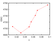
(b)

Figure 2: (a) Variation of the sparsity obtained with FDR for different values of $\alpha$ and (b) Variation of EBIC for the selected values of $\alpha$ ($p=30$ , $n=40$ and $80\%$ sparsity).

(a)

(b)

Figure 3: Variation of the objective function with (a) iteration index and (b) Time (seconds) for $p=20$ and $n=40$ .

III-A1 Choosing $\alpha$

To illustrate the choice of $\alpha$, we cover the interval $\left[0.01,0.1\right]$ using a fine grid with a step of $0.005$ and obtain the sparsity corresponding to each grid point using the FDR. Fig. 2(a) shows the sparsity vs $\alpha$ plot for an example where $p=30$, $n=40$ and the sparsity of the true covariance matrix is $80\%$. From the figure it can be observed that the variation of sparsity with $\alpha$ is step-wise. Also, the corresponding sparsity patterns are hierarchical (see Section II-A2). In particular, this means that the same sparsity level implies the same sparsity pattern, which allows us to evaluate EBIC only at a small number of points in the interval, thereby reducing the computational burden of choosing a value for $\alpha$. We pick one value of $\alpha$ for each sparsity level and evaluate EBIC at these points. Fig. 2(b) shows the variation of EBIC versus the selected values of $\alpha$ . The value of $\alpha$ that yields the lowest value of the criterion is chosen. Note from Fig. 2(b) that in the present case we had to compute the MLE of $\boldsymbol{\Sigma}$ only for seven values of $\alpha$ (i.e., seven sparsity patterns).

III-A2 Comparison of PD with the algorithm proposed in [28]

Fig. 3(a) shows the variation of the objective function versus the iteration index for both methods. The two algorithms are run on the same problem (7) for the choice of $k=40$. We can see from the figure that the proposed PD method converges to a lower value of the objective function than the method in [28] does. This difference can be attributed to the fact that the surrogate in [28] is not a real upper bound on the objective function whereas the surrogate used in the PD tightly upperbounds the objective function. The plot of the objective function versus time is shown in Fig. 3(b) for both methods. Note that the time complexity of PD is comparable to that of the method in [28]. However the comparison in the latter figure does not include the time needed for choosing the hyper-parameter for either method, which can be potentially much larger for the method of [28] (as explained before).

III-A3 BCD vs PD

Next we compare the performance of the two methods proposed in this paper in terms of their computational complexity and convergence. Fig. 4 shows the variation of the objective function with the iteration index, whereas Fig. 5 shows the variation versus time. From Fig. 4 we can see that PD converges to the same solution as BCD if the penalty parameter is properly tuned. However if $\zeta$ is not chosen correctly, the algorithm converges to sub-optimal values. From Fig. 5 it can be observed that PD with the a proper choice of $\zeta$ is not only capable of converging to the same solution as BCD, but can be faster than BCD. However, because the tuning of the penalty parameter $\zeta$ is not simple, in the subsequent examples we will use only BCD.

Figure 4: Objective function vs iteration for $p=30$, $n=40$ and $\textrm{sparsity}=75\%$

Figure 5: Objective function vs time (s) for $p=30$, $n=40$ and $\textrm{sparsity}=75\%$

III-A4 The effect of sparsity

We study the effect of sparsity of the true covariance matrix on the performance of BCD in terms of the normalized root mean square error (NRMSE):

$$\textrm{NRMSE}=\left\|\mathbf{\boldsymbol{\Sigma}}_{\textrm{true}}-\hat{\mathbf{\boldsymbol{\Sigma}}}\right\|_{F}/\left\|\mathbf{\boldsymbol{\Sigma}}_{\textrm{true}}\right\|_{F}.$$ (62)

Fig. 6 shows the variation of NRMSE with the sparsity. The dashed curves show the NRMSE obtained by solving the constrained problem (21) with the matrix $\mathbf{Z}$ in the constraint inferred via FDR (with $\alpha$ chosen via EBIC), whereas the solid curves show the NRMSE obtained from (21) where $\mathbf{Z}$ corresponds to the sparsity pattern of $\mathbf{\boldsymbol{\Sigma}}_{\textrm{true}}$. As expected the NRMSE is lower when $\mathbf{Z}$ encodes the true sparsity pattern. However, the performance difference is not large especially if $n>p$. Also, once again as expected, the NRMSE decreases as sparsity of $\mathbf{\boldsymbol{\Sigma}}_{\textrm{true}}$ increases.

Figure 6: NRMSE vs sparsity for $p=30$. The dashed curves show the NRMSE obtained with the sparsity pattern inferred via FDR and the solid curves show the NRMSE obtained with the true sparsity pattern.

III-A5 Comparison with two state-of-the-art methods

Lastly, we compare BCD with SCM and the state-of-the-art methods of [25] and [28]. Fig. 7 shows the variation of NRMSE with the number of samples $n$ for $p=150$ and $n$ between $100$ and 2$00$. The true covariance matrix has a sparsity of $66\%$. From the figure we can see that BCD yields a lower value of NRMSE (with a difference of above $10\%$ or more) for all values of $n$.

Figure 7: Variation of NRMSE with number of samples ($n)$ for $p=150$ and sparsity $=66\%$.

We also use the Matthews correlation coefficient (MCC) to evaluate the performance of the proposed algorithms w.r.t. recovering the true covariance graph structure. MCC is defined as [45]:

$$\small\textrm{MCC}=\frac{TP.TN-FP.FN}{\sqrt{(TP+FP)(TP+FN)(TN+FP)(TN+FN)}},$$ (63)

where $TP$, $TN$, $FP$, and $FN$ denote the number of true positives, true negatives, false positives and false negatives, see the so-called confusion matrix given in Table I. A higher value of MCC signifies fewer false alarms and misses, and therefore a better performance. Fig. 8 shows the variation of MCC with the number of samples for $p=30$ and a true covariance matrix with sparsity $75\%$. It can be seen that BCD has the highest MCC scores.

In both the experiments, the value of $\alpha$ for BCD is estimated using EBIC, the regularization parameter $\lambda$ in [25] is chosen by a rather time consuming cross-validation operation, whereas $k$ in [28] is chosen equal to the number of nonzero entries in the upper triangle of the true covariance matrix (a choice that of course would not be feasible in applications).

TABLE I: Confusion matrix

	$H_{ij}$ = accepted	$H_{ij}$ = rejected
	($\hat{\Sigma}_{ij}=0$)	($\hat{\Sigma}_{ij}\neq 0$)
$H_{ij}$ = true	$TN$	$FP$
($\Sigma_{ij}=0$)	(detection)	(false alarm)
$H_{ij}$ = false	$FN$	$TP$
($\Sigma_{ij}\neq 0$)	(miss)	(detection)

Figure 8: MCC vs the number of samples ($n$) for $p=30$, sparsity$=75\%$ and $n$ varying between $50$ and $500$.

III-B Real data

To test the performance of BCD on real data we consider two datasets: international migration forecast data that consist of the net migration estimates in different countries and cell signalling data that consist of the flow cytometry measurements of proteins in the cells.

(a)	(d)
(b)	(e)
(c)	(f)

Figure 9: Two examples of estimated correlations of five countries. Example 1 (left-hand side): (a) Pearson correlation estimates; (b) EBIC vs $\alpha$; (c) Estimated correlations using BCD ($\alpha=0.002$). Example 2 (right-hand side): (a) Pearson correlation estimates; (b) EBIC vs $\alpha$; (c) Estimated correlations using BCD ($\alpha=0.065$)

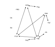
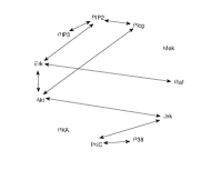
(a)	(b)	(c)	(d)

Figure 10: (a) Estimated covariance graphs obtained using BCD; (b) Markov graphs obtained using the Graphical Lasso for precision matrix estimation; (c) Estimated covariance graphs obtained using the method of [28]; (d) Estimated covariance graphs obtained using the method of [25]. First row: $k=16$ edges, second row: $k=9$ edges and third row: $k=6$ edges.

III-B1 Migration data

Estimating correlations of migration forecast errors for different countries helps yielding more accurate estimates and projections of international migration, which is important for policy making at a country level. The 2012 revision of the international migration data (as used in [28]) from the United Nations World Population Prospects division consist of net migration rate estimates in each country every five years starting from 1950 ($12$ measurements). Following [28], we determine the residual errors for net migration between all countries using an AR(1) model that yields $n=11$ observed samples, and estimate the covariance matrix for $p=5$ countries chosen from the total of $191$ countries. From the estimated covariance matrix, we determine the correlation across the chosen countries. For the purpose of illustration, we first choose the following five countries: Estonia, Latvia, Lithuania (northern Europe region), Vietnam (South-eastern Asia), and Hong Kong (Eastern Asia). Fig. 9(a) shows the heatmap of the Pearson correlation estimates obtained using SCM for this set of countries. In Fig. 9(b) we show the variation of EBIC with $\alpha$ for this example and find that the recommended $\alpha$ lies anywhere between $0.002$ and $0.07$. Using $\alpha=0.002$ we obtain the correlation matrix with BCD and show it in Fig 9(c). The non-zero values of the correlation estimates between the country pairs Latvia-Estonia and Latvia-Lithuania is probably due to the fact that Latvia shares borders with both Estonia and Lithuania. We also consider a second set of five countries: Bahamas, Puerto Rico, Jamaica (Caribbean), Zambia and Zimbabwe (Eastern Africa). Figs. 9(d)-(f) show their Pearson correlation estimates, the variation of EBIC with $\alpha$, and the correlation estimates obtained via BCD with $\alpha=0.065$. From Fig. 9(f), we observe that the non-zero entries estimated with BCD correspond to the country pairs that belong to the same region of the UN world partition. Additionally it is found that Puerto Rico is uncorrelated to Jamaica and Bahamas, even though they are in the same region of the UN world partition. This can mainly be attributed to Puerto Rico being an unincorporated territory of the United States, whereas Jamaica and Bahamas being independent nations. Moreover, the official language of Puerto Rico is Spanish and English, with Spanish being the predominant language in the island. On the other hand, both Jamaica and Bahamas have English as their official language, with most people speaking English or English-based creoles.

III-B2 Cell signalling data

The cell signalling dataset [46] has been previously studied in the context of sparse covariance estimation by the authors of [25] and [28]. The data contain the flow cytometry measurements of $p=11$ proteins in $n=7466$ cells. A missing edge between two proteins in the covariance graph suggests that the concentration of one protein gives no information about the concentration of the other protein.

We estimate the covariance matrix with different sparsity levels for the flow cytometry measurements using BCD (different sparsity levels in the covariance matrix are obtained using different values of $\alpha$). The corresponding covariance graphs with $k=16,9$ and $6$ edges are shown in the first column of Fig. 10. We compare these estimated covariance graphs with the Markov graphs (with the same number of edges), as shown in the second column of Fig. 10, which are undirected graphs obtained by solving the graphical Lasso problem for precision matrix estimation. Since a missing edge in the Markov graph indicates conditional independence between two variables, as opposed to marginal independence in the case of a covariance graph, the two graphs are not completely identical. However, as shown in the figure, the covariance graph obtained via BCD is quite similar to the Markov graph, and this similarity increases as the number of edges decreases (with completely identical graphs when $k=9$ and $6$). The third and the fourth column of the figure show the covariance graphs obtained using the methods in [28] and [25]. The covariance graphs using the method of [28] is also similar to the Markov graph (the covariance graphs obtained with BCD have a larger number of edges in common with the Markov graphs), whereas the covariance graphs obtained using the method of [25] are quite different from the Markov graphs.

Figure 11: Estimated covariance graph using BCD with the value of $\alpha$ ($0.004)$ obtained via EBIC.

We also estimate the covariance matrix using BCD with $\alpha$ obtained via EBIC, the covariance graph of which is shown in Fig. 11. This estimated covariance graph has a sparsity of $58\%$ and $23$ edges.

IV Conclusions

In this paper we have presented two methods for estimating sparse covariance matrices. The proposed methods estimate the sparsity pattern of the target covariance matrix using FDR multiple hypothesis testing before solving the MLE problem via two different algorithms. The first block coordinate descent method does not require the tuning of any hyper-parameter, whereas the second proximal distance method is computationally fast but requires the careful tuning of a hyper-parameter. We tested the proposed algorithms on both synthetically generated and real-world data, and compared them with two state-of-the-art methods.

References

- [1] D. M. Witten and R. Tibshirani, “Penalized classification using fisher’s linear discriminant,” Journal of the Royal Statistical Society: Series B (Statistical Methodology), vol. 73, no. 5, pp. 753–772, 2011.
- [2] P. Stoica and R. L. Moses, Spectral analysis of signals. Pearson Prentice Hall, 2005.
- [3] J. Schäfer and K. Strimmer, “A shrinkage approach to large-scale covariance matrix estimation and implications for functional genomics,” Statistical applications in genetics and molecular biology, vol. 4, no. 1, 2005.
- [4] T. Soderstrom and P. Stoica, System identification. Prentice-Hall, 1989.
- [5] A. Aubry, A. De Maio, and L. Pallotta, “A geometric approach to covariance matrix estimation and its applications to radar problems,” IEEE Transactions on Signal Processing, vol. 66, no. 4, pp. 907–922, 2017.
- [6] O. Ledoit and M. Wolf, “Honey, I shrunk the sample covariance matrix,” The Journal of Portfolio Management, vol. 30, no. 4, pp. 110–119, 2004.
- [7] L. Yang, R. Couillet, and M. R. McKay, “A robust statistics approach to minimum variance portfolio optimization,” IEEE Transactions on Signal Processing, vol. 63, no. 24, pp. 6684–6697, 2015.
- [8] S. Deshmukh and A. Dubey, “Improved covariance matrix estimation with an application in portfolio optimization,” IEEE Signal Processing Letters, vol. 27, pp. 985–989, 2020.
- [9] M. Senneret, Y. Malevergne, P. Abry, G. Perrin, and L. Jaffres, “Covariance versus precision matrix estimation for efficient asset allocation,” IEEE Journal of Selected Topics in Signal Processing, vol. 10, no. 6, pp. 982–993, 2016.
- [10] H. Toh and K. Horimoto, “Inference of a genetic network by a combined approach of cluster analysis and graphical gaussian modeling,” Bioinformatics, vol. 18, no. 2, pp. 287–297, 2002.
- [11] J. Schäfer and K. Strimmer, “An empirical bayes approach to inferring large-scale gene association networks,” Bioinformatics, vol. 21, no. 6, pp. 754–764, 2005.
- [12] O. Banerjee, L. El Ghaoui, and A. d’Aspremont, “Model selection through sparse maximum likelihood estimation for multivariate gaussian or binary data,” The Journal of Machine Learning Research, vol. 9, pp. 485–516, 2008.
- [13] M. O. Kuismin and M. J. Sillanpää, “Estimation of covariance and precision matrix, network structure, and a view toward systems biology,” Wiley Interdisciplinary Reviews: Computational Statistics, vol. 9, no. 6, p. e1415, 2017.
- [14] D. Cox and N. Wermuth, Multivariate Dependencies: Models, Analysis and Interpretation, vol. 67. CRC Press, 1996.
- [15] W. B. Wu and M. Pourahmadi, “Nonparametric estimation of large covariance matrices of longitudinal data,” Biometrika, vol. 90, no. 4, pp. 831–844, 2003.
- [16] P. J. Bickel and E. Levina, “Regularized estimation of large covariance matrices,” The Annals of Statistics, vol. 36, no. 1, pp. 199–227, 2008.
- [17] R. Furrer and T. Bengtsson, “Estimation of high-dimensional prior and posterior covariance matrices in kalman filter variants,” Journal of Multivariate Analysis, vol. 98, no. 2, pp. 227–255, 2007.
- [18] T. T. Cai, C.-H. Zhang, and H. H. Zhou, “Optimal rates of convergence for covariance matrix estimation,” The Annals of Statistics, vol. 38, no. 4, pp. 2118–2144, 2010.
- [19] N. El Karoui, “Operator norm consistent estimation of large-dimensional sparse covariance matrices,” The Annals of Statistics, vol. 36, no. 6, pp. 2717–2756, 2008.
- [20] A. J. Rothman, E. Levina, and J. Zhu, “Generalized thresholding of large covariance matrices,” Journal of the American Statistical Association, vol. 104, no. 485, pp. 177–186, 2009.
- [21] P. J. Bickel and E. Levina, “Covariance regularization by thresholding,” The Annals of statistics, vol. 36, no. 6, pp. 2577–2604, 2008.
- [22] T. Cai and W. Liu, “Adaptive thresholding for sparse covariance matrix estimation,” Journal of the American Statistical Association, vol. 106, no. 494, pp. 672–684, 2011.
- [23] A. J. Rothman, “Positive definite estimators of large covariance matrices,” Biometrika, vol. 99, no. 3, pp. 733–740, 2012.
- [24] L. Xue, S. Ma, and H. Zou, “Positive-definite 1-penalized estimation of large covariance matrices,” Journal of the American Statistical Association, vol. 107, no. 500, pp. 1480–1491, 2012.
- [25] J. Bien and R. J. Tibshirani, “Sparse estimation of a covariance matrix,” Biometrika, vol. 98, no. 4, pp. 807–820, 2011.
- [26] H. Wang, “Coordinate descent algorithm for covariance graphical lasso,” Statistics and Computing, vol. 24, no. 4, pp. 521–529, 2014.
- [27] D. N. Phan, H. A. Le Thi, and T. P. Dinh, “Sparse covariance matrix estimation by DCA-based algorithms,” Neural Computation, vol. 29, no. 11, pp. 3040–3077, 2017.
- [28] J. Xu and K. Lange, “A proximal distance algorithm for likelihood-based sparse covariance estimation,” Biometrika, vol. 109, no. 4, pp. 1047–1066, 2022.
- [29] M. Grant and S. Boyd, “CVX: Matlab software for disciplined convex programming, version 2.1.” http://cvxr.com/cvx, Mar. 2014.
- [30] J. Friedman, T. Hastie, and R. Tibshirani, “Sparse inverse covariance estimation with the graphical lasso,” Biostatistics, vol. 9, no. 3, pp. 432–441, 2008.
- [31] M. Drton and T. S. Richardson, “A new algorithm for maximum likelihood estimation in gaussian graphical models for marginal independence,” in Proceedings of the 19th Conference Annual Conference on Uncertainty in Artificial Intelligence (UAI-03), pp. 184–191, 2003.
- [32] S. Chaudhuri, M. Drton, and T. S. Richardson, “Estimation of a covariance matrix with zeros,” Biometrika, vol. 94, no. 1, pp. 199–216, 2007.
- [33] A. J. Butte, P. Tamayo, D. Slonim, T. R. Golub, and I. S. Kohane, “Discovering functional relationships between rna expression and chemotherapeutic susceptibility using relevance networks,” Proceedings of the National Academy of Sciences, vol. 97, no. 22, pp. 12182–12186, 2000.
- [34] M. Grzebyk, P. Wild, and D. Chouanière, “On identification of multi-factor models with correlated residuals,” Biometrika, vol. 91, no. 1, pp. 141–151, 2004.
- [35] O. J. Dunn and V. A. Clark, Applied statistics: analysis of variance and regression. John Wiley & Sons, Inc., 1986.
- [36] A. Rahman, N., A course in theoretical statistics. Charles Griffin and Company, 1968.
- [37] Y. Benjamini and Y. Hochberg, “Controlling the false discovery rate: a practical and powerful approach to multiple testing,” Journal of the Royal statistical society: series B (Methodological), vol. 57, no. 1, pp. 289–300, 1995.
- [38] Y. Benjamini and D. Yekutieli, “The control of the false discovery rate in multiple testing under dependency,” Annals of statistics, pp. 1165–1188, 2001.
- [39] J. Chen and Z. Chen, “Extended Bayesian information criteria for model selection with large model spaces,” Biometrika, vol. 95, no. 3, pp. 759–771, 2008.
- [40] Y. Sun, P. Babu, and D. P. Palomar, “Majorization-minimization algorithms in signal processing, communications, and machine learning,” IEEE Transactions on Signal Processing, vol. 65, no. 3, pp. 794–816, 2016.
- [41] K. L. Keys, H. Zhou, and K. Lange, “Proximal distance algorithms: Theory and practice,” The Journal of Machine Learning Research, vol. 20, no. 1, pp. 2384–2421, 2019.
- [42] A. Ruhe, “Perturbation bounds for means of eigenvalues and invariant subspaces,” BIT Numerical Mathematics, vol. 10, no. 3, pp. 343–354, 1970.
- [43] P. Stoica and P. Babu, “Low-rank covariance matrix estimation for factor analysis in anisotropic noise: application to array processing and portfolio selection,” arXiv preprint arXiv:2304.08813, 2023.
- [44] P. Tseng, “Convergence of a block coordinate descent method for nondifferentiable minimization,” Journal of optimization theory and applications, vol. 109, no. 3, p. 475, 2001.
- [45] B. W. Matthews, “Comparison of the predicted and observed secondary structure of t4 phage lysozyme,” Biochimica et Biophysica Acta (BBA)-Protein Structure, vol. 405, no. 2, pp. 442–451, 1975.
- [46] K. Sachs, O. Perez, D. Pe’er, D. A. Lauffenburger, and G. P. Nolan, “Causal protein-signaling networks derived from multiparameter single-cell data,” Science, vol. 308, no. 5721, pp. 523–529, 2005.