How Expressive are Spectral-Temporal Graph Neural Networks for Time Series Forecasting?

Abstract

Spectral-temporal graph neural network is a promising abstraction underlying most time series forecasting models that are based on graph neural networks (GNNs). However, more is needed to know about the underpinnings of this branch of methods. In this paper, we establish a theoretical framework that unravels the expressive power of spectral-temporal GNNs. Our results show that linear spectral-temporal GNNs are universal under mild assumptions, and their expressive power is bounded by our extended first-order Weisfeiler-Leman algorithm on discrete-time dynamic graphs. To make our findings useful in practice on valid instantiations, we discuss related constraints in detail and outline a theoretical blueprint for designing spatial and temporal modules in spectral domains. Building on these insights and to demonstrate how powerful spectral-temporal GNNs are based on our framework, we propose a simple instantiation named Temporal Graph GegenConv (TGC), which significantly outperforms most existing models with only linear components and shows better model efficiency.

1 Introduction

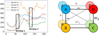
Figure 1: Differently signed spatial relations between time series in PeMS07 dataset. Left: Visualization of four randomly selected traffic sensor readings. Right: Spatial relations between time series may be different in two windows (e.g., A and D are positively and negatively correlated in windows 1 and 2, respectively).

Graph neural networks (GNNs) have achieved considerable success in static graph representation learning for many tasks [1]. Many existing studies, such as STGCN [2] and Graph WaveNet [3], have successfully extended GNNs to time series forecasting. Among these methods, either first-order approximation of ChebyConv [4] or graph diffusion [5] is typically used to model time series relations, where a strong assumption of local homophiles is made [6]. Thus, they are only capable of modeling positive correlations between time series that exhibit strong similarities, and we denote this branch of methods as message-passing-based spatial-temporal GNNs (MP-STGNNs). Nevertheless, how to model real-world multivariate time series with complex spatial dependencies that evolve remains an open question. This complexity is depicted in Figure 1, in which differently signed relations between time series are evident.

Recently, Cao et al. [7] introduced the concept of spectral-temporal GNNs (SPTGNNs), which sheds light on modeling differently signed time series correlations by approximating graph convolutions with a broad range of graph spectral filters beyond low-pass filtering [8, 9]. Though StemGNN [7] has achieved remarkable improvements in time series forecasting, the theoretical foundations of SPTGNNs remain under-researched. There are several unresolved fundamental questions: Q1. What is the general form of SPTGNNs? Q2. How expressive are SPTGNNs? Q3. When will they fail to generalize well? Q4. How to design provably expressive SPTGNNs?

We establish a series of theoretical results (summarized in Figure 2) to answer these questions. We begin by formulating a general framework of SPTGNNs (Q1; subsection 3.1), and then prove its universality of linear models (i.e., linear SPTGNNs are powerful enough to represent arbitrary time series) under mild assumptions through the lens of discrete-time dynamic graphs (DTDGs) [10] and spectral GNNs [13]. We further discuss related constraints from various aspects (Q3; subsection 3.2) to make our theorem useful in practice on any valid instantiations. After this, we extend the color-refinement algorithm on DTDGs and prove that the expressive power of SPTGNNs is theoretically bounded by the proposed temporal 1-WL test (Q2; subsection 3.2). To answer the last question (Q4; subsection 3.3), we prove that under mild assumptions, linear SPTGNNs are sufficient to produce expressive time series representations with orthogonal function bases and individual spectral filters in their graph and temporal frequency-domain models. Our results, for the first time, unravel the learning capabilities of SPTGNNs and outline a blueprint for designing powerful GNN-based forecasting models.

Figure 2: Venn diagram of our method and overview of our contributions.

Drawing from and to validate these theoretical insights, we present a simple SPTGNN instantiation, named TGC (short for Temporal Graph GegenConv), that well generalizes related work in time series forecasting. Though our primary goal is not to achieve state-of-the-art performance, our method, remarkably, is very efficient and significantly outperforms numerous existing models on several time series benchmarks and forecasting settings with minimal designs. Comprehensive experiments on synthetic and real-world datasets demonstrate that: (1) Our approach excels at learning time series relations of different types compared to MP-STGNNs; (2) Our design principles, e.g., orthogonal bases and individual filtering, are crucial for SPTGNNs to perform well; (3) Our instantiation (TGC) can be readily augmented with nonlinearities and other common model choices. Finally, and more importantly, our findings pave the way for devising a broader array of provably expressive SPTGNNs.

2 Preliminaries

In time series forecasting, given a series of historical observations $\mathbf{X}\in\mathbb{R}^{N\times T\times D}$ encompassing $N$ different $D$-dimensional variables across $T$ time steps, we aim to learn a function $f(\cdot):\mathbf{X}\mapsto\hat{\mathbf{Y}}$, where the errors between the forecasting results $\hat{\mathbf{Y}}\in\mathbb{R}^{N\times H\times D}$ and ground-truth $\mathbf{Y}$ are minimized with the following mean squared loss: $\frac{1}{H}\sum_{t=1}^{H}||\hat{\mathbf{Y}}_{t}-\mathbf{Y}_{t}||^{2}_{F}$. $H$ denotes the forecasting horizon.

In this work, we learn an adjacency matrix $\mathbf{A}\in\mathbb{R}^{N\times N}$ from the input window $\mathbf{X}$ to describe the connection strength between $N$ variables, as in [7]. Specifically, we use $\mathbf{X}_{t}:=\mathbf{X}_{:,t,:}\in\mathbb{R}^{N\times D}$ to denote the observations at a specific time $t$, and $\mathbf{X}_{n}:=\mathbf{X}_{n,:,:}\in\mathbb{R}^{T\times D}$ as a time series of a specific variable $n$ with $T$ time steps and $D$ feature dimensions. Detailed preliminaries are in Appendix A.

Graph Spectral Filtering.

For simplicity and modeling the multivariate time series from the graph perspective, we let $\mathcal{G}_{t}=(\mathbf{A},\mathbf{X}_{t})$ denote an undirected graph snapshot at a specific time $t$ with the node features $\mathbf{X}_{t}$. In a graph snapshot, $\mathbf{A}$ and its degree matrix $\mathbf{D}\in\mathbb{R}^{N\times N}$ s.t. $\mathbf{D}_{i,i}=\sum_{j=1}^{N}\mathbf{A}_{i,j}$; thus, its normalized graph Laplacian matrix $\hat{\mathbf{L}}=\mathbf{D}^{-\frac{1}{2}}(\mathbf{D}-\mathbf{A})\mathbf{D}^{-\frac{1}{2}}$ is symmetric and can be proven to be positive semi-definite. We let the eigendecomposition of $\mathcal{G}_{t}$ to be $\hat{\mathbf{L}}=\mathbf{U}\mathbf{\Lambda}\mathbf{U}^{\top}$. Below, we define graph convolution to filter input signal in the spectral domain w.r.t. node connectivity.

Definition 1 (Graph Convolution).

Assume there is a filter function of eigenvalues $g(\cdot):[0,2]\mapsto\mathbb{R}$, we define the graph convolution on $\mathcal{G}_{t}$ as filtering the input signal $\mathbf{X}_{t}$ with the spectral filter:

$$g(\mathbf{\Lambda})\star\mathbf{X}_{t}:=\mathbf{U}g(\mathbf{\Lambda})\mathbf{U}^{\top}\mathbf{X}_{t}.$$ (1)

Directly computing Equation 1 is costly. We approximate the learnable filter function $g_{\theta}(\mathbf{\Lambda})$ with a truncated $K$-degree polynomial expansion: $g_{\theta}(\lambda):=\sum_{k=0}^{K}\mathbf{\Theta}_{k,:}P_{k}(\lambda)$; thus, the graph spectral filtering takes the form of $\mathbf{U}g_{\theta}(\mathbf{\Lambda})\mathbf{U}^{\top}\mathbf{X}_{t}\!:=\!\sum_{k=0}^{K}\mathbf{\Theta}_{k,:}\mathbf{U}P_{k}(\mathbf{\Lambda})\mathbf{U}^{\top}\mathbf{X}_{t}\!=\!\!\sum_{k=0}^{K}\mathbf{\Theta}_{k,:}P_{k}(\hat{\mathbf{L}})\mathbf{X}_{t}$. If $g_{\theta}(\hat{\mathbf{L}})=\sum_{k=0}^{K}\mathbf{\Theta}_{k,:}P_{k}(\hat{\mathbf{L}})$, we have the graph convolution redefined as: $g(\mathbf{\Lambda})\star\mathbf{X}_{t}:=g_{\theta}(\hat{\mathbf{L}})\mathbf{X}_{t}$.

Orthogonal Time Series Representations.

Time series can be analyzed in both time and spectral domains. In this work, we focus on modeling time series using sparse orthogonal representations. Specifically, for an input signal of the $n^{\text{th}}$ variable, we represent $\mathbf{X}_{n}$ by a set of orthogonal components $\tilde{\mathbf{X}}_{n}$. We provide further details in Appendix A, discussing discrete Fourier transformation (DFT) and other applicable space projections with orthogonal bases.

3 Spectral-Temporal Graph Neural Networks

We address all research questions in this section. We first introduce the general form of SPTGNNs and then unravel the expressive power of this family of methods. On this basis, we further shed light on the design of powerful SPTGNNs with theoretical proofs.

3.1 Formulation

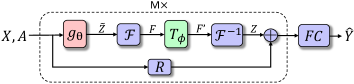
Figure 3: The general formulation of SPTGNNs with $M$ building blocks to predict future values $\hat{\mathbf{Y}}$ based on historical observations $\mathbf{X}$. $g_{\theta}(\cdot)$ and $\mathcal{T}_{\phi}(\cdot)$ are graph and temporal spectral filters. $\mathcal{F}(\cdot)$ and $\mathcal{F}^{-1}(\cdot)$ are forward and inverse space projectors.

Overall Architecture.

We illustrate the general framework of SPTGNNs in Figure 3, where we stack $M$ building blocks to capture spatial and temporal dependencies in spectral domains. Without loss of generality, we formulate this framework with the minimum redundancy and a straightforward optimization objective, where common add-ons in prior arts, e.g., spectral attention [14], can be easily incorporated. To achieve time series connectivity without prior knowledge, we directly use the latent correlation layer from [7], as this is not our primary focus.

Building Block.

From the graph perspective and given the adjacency matrix $\mathbf{A}$, we can view the input signal $\mathbf{X}$ as a particular DTDG with a sequence of regularly-sampled static graph snapshots $\{\mathcal{G}_{t}\}_{t=0}^{T-1}$, where node features evolve but with fixed graph topology. In a SPTGNN block, we filter $\mathbf{X}$ from the spatial and temporal perspectives in spectral domains with graph spectral filters (GSFs) and temporal spectral filters (TSFs). Formally, considering a single dimensional input $\mathbf{X}_{d}:=\mathbf{X}_{:,:,d}\in\mathbb{R}^{N\times T}$, we define a SPTGNN block as follows without the residual connection:

$$\mathbf{Z}_{d}=\mathcal{T}_{\phi_{d}}\Big{(}g_{\theta_{d}}(\hat{\mathbf{L}})\mathbf{X}_{d}\Big{)}=\mathcal{T}_{\phi_{d}}\Big{(}\sum_{k=0}^{K}\mathbf{\Theta}_{k,d}P_{k}(\hat{\mathbf{L}})\mathbf{X}_{d}\Big{)}.$$ (2)

This formulation is straightforward. $\mathcal{T}_{\phi}(\cdot)$ represents TSFs, which work in conjunction with space projectors (detailed in subsection 3.3) to model temporal dependencies between node embeddings across snapshots. The internal expansion corresponds to GSFs’ operation, which embeds node features in each snapshot $\mathcal{G}_{t}$ by learning variable relations. The above process can be understood in different ways. The polynomial bases and coefficients generate distinct GSFs, allowing the internal $K$-degree expansion in Equation 2 to be seen as a combination of different dynamic graph profiles at varying hops in the graph domain. Each profile filters out a specific frequency signal. Temporal dependencies are then modeled for each profile before aggregation: $\mathbf{Z}_{d}=\sum_{k=0}^{K}\mathcal{T}_{\phi_{d}}\Big{(}\mathbf{\Theta}_{k,d}P_{k}(\hat{\mathbf{L}})\mathbf{X}_{d}\Big{)}$, which is equivalent to our formulation. Alternatively, dynamic graph profiles can be formed directly in the spectral domain, resulting in the formulation in StemGNN [7] with increased model complexity.

3.2 Expressive Power of Spectral-Temporal GNNs

In this section, we develop a theoretical framework bridging spectral and dynamic GNNs, elucidating the expressive power of SPTGNNs for modeling time series data. All proofs are in Appendix C.

Linear GNNs.

For a linear GNN on $\mathbf{X}\in\mathbb{R}^{N\times D}$, we define it using a trainable weight matrix $\mathbf{W}$ and parameterized spectral filters $g_{\theta}(\hat{\mathbf{L}})$ as $\tilde{\mathbf{Z}}=g_{\theta}(\hat{\mathbf{L}})\mathbf{X}\mathbf{W}$. This simple linear GNN can express any polynomial filter functions, denoted as Polynomial-Filter-Most-Expressive (PFME), under mild assumptions [13]. Its expressiveness establishes a lower bound for spectral GNNs.

To examine the expressive power of SPTGNNs, we generalize spectral GNNs to model dynamic graphs. For simplicity, we initially consider linear GNNs with a single linear mapping $f_{\phi}(\cdot)$. To align with our formulation, $\mathcal{T}_{\phi}(\cdot)$ should also be linear functions; thus, Equation 2 can be interpreted as a linear GNN extension, where $f_{\phi}(\cdot)$ depends on historical observations instead of a graph snapshot. Accordingly, linear SPTGNNs establish a lower bound for the expressive power of SPTGNNs.

Proposition 1.

A SPTGNN can differentiate any pair of nodes at an arbitrary valid time that linear SPTGNNs can if $\mathcal{T}_{\phi}(\cdot)$ can express any linear time-variant functions.

Despite their simplicity, linear SPTGNNs maintain the fundamental spectral filtering forms of SPTGNNs. We begin by defining the universal approximation theorem for linear SPTGNNs.

Theorem 1.

A linear SPTGNN can produce arbitrary dimensional time series representations at any valid time iff: (1) $\hat{\mathbf{L}}$ has no repeated eigenvalues; (2) $\mathbf{X}$ encompasses all frequency components with respect to the graph spectrum; (3) $\mathcal{T}_{\phi}(\cdot)$ can express any single-dimensional univariate time series.

Next, we separately explore these conditions and relate them to practical spectral-temporal GNNs.

Multidimensional and Multivariate Prediction.

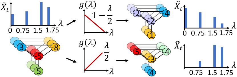
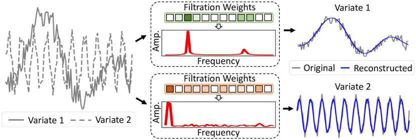
Figure 4: Multidimensional and multivariate predictions. Left: Multidimensional predictions within a snapshot require individual filtration for each output dimension to preserve different information. Right: Individual filter is needed to model each single-dimensional time series.

In a graph snapshot, each dimension may exhibit different properties, necessitating distinct filters for processing [13]. An example with two-dimensional predictions is provided in Figure 4. A simple solution involves using multidimensional polynomial coefficients, as explicitly shown in Equation 2. A concrete example is presented in [8], where given a series of Bernstein bases, different polynomial coefficients result in various Bernstein approximations, corresponding to distinct GSFs. Similarly, when modeling temporal clues between graph snapshots, either dimension in any variable constitutes a unique time series requiring a specific filtering. An example reconstructing a two-variate time series of one dimension is in Figure 4. In practice, we use multidimensional masking and weight matrices for each variable, forming a set of different TSFs. This is discussed in subsection 3.3.

Missing Frequency Components and Repeated Eigenvalues.

GSFs can only scale existing frequency components of specific eigenvalues. For each graph snapshot, linear SPTGNNs cannot generate new frequency components if certain frequencies are missing from the original graph spectrum. For instance, in Figure 4, a frequency component corresponding to $\lambda=1$ cannot be generated with a spectral filter. Although this issue is challenging to address, it is rare in real-world attributed graphs [13]. In a graph with repeated eigenvalues given its topology, multiple frequency components will be scaled by the same $P_{k}(\lambda)$, thus affecting spectral filtering.

Universal Temporal Spectral Filtering.

For a finite-length one-dimensional univariate time series, it can be provably modeled using a frequency-domain model (FDM), consisting of sparse orthogonal space projectors and spectral filters. Figure 4 exemplifies modeling two time series with distinct TSFs. Further details are discussed in subsection 3.3.

Nonlinearity.

Nonlinear activation can be applied in both GSFs and TSFs. In the first case, we examine the role of nonlinearity over the spatial signal, i.e., $\sigma(\mathbf{X}_{t})$, enabling frequency components to be mixed w.r.t. the graph spectrum [13]. In the second case, we investigate the role of nonlinearity over the temporal signal by studying its equivalent effect $\sigma^{\prime}(\cdot)$, as $\sigma(\mathbf{X}_{n})=\mathcal{F}^{-1}\big{(}\sigma^{\prime}(\mathcal{F}(\mathbf{X}_{n}))\big{)}$. Here, we have $\sigma^{\prime}(\tilde{\mathbf{X}}_{n})=\mathcal{F}\big{(}\sigma(\mathcal{F}^{-1}(\tilde{\mathbf{X}}_{n}))\big{)}$, where different components in $\tilde{\mathbf{X}}_{n}$ are first mixed (e.g., via Equation S6) and then element-wise transformed by a nonlinear function $\sigma(\cdot)$ before being redistributed (e.g., via Equation S5). Consequently, a similar mixup exists, allowing different components to transform into each other in an orthogonal space.

Connection to Dynamic Graph Isomorphism.

Analyzing the expressive power of GNNs is often laid on graph isomorphism. In this context, we first define the temporal Weisfeiler-Lehman (WL) test and subsequently establish a connection to linear SPTGNNs in Theorem 2.

Definition 2 (Temporal 1-WL test).

Temporal 1-WL test on discrete-time dynamic graphs $\mathcal{G}:=\{\mathcal{G}_{t}\}_{t=0}^{T-1}$ with a fixed node set $\mathbb{V}$ is defined below with iterative graph coloring procedures:

Initialization: All node colors are initialized using node features. In a snapshot at time $t$, we have $\forall v\in\mathbb{V},c^{(0)}(v,t)=\mathbf{X}_{t}[v]$. In the absence of node features, all nodes get the same color.

Iteration: At step $l$, node colors are updated with an injective (hash) function: $\forall v\in\mathbb{V},t\in[1,T),c^{(l+1)}(v,t)=\textsc{Hash}(c^{(l)}(v,t),c^{(l)}(v,t-1),\{\!\!\{c^{(l)}(u,t):e_{u,v,t}\in\mathbb{E}(\mathcal{G}_{t})\}\!\!\})$. When $t=0$ or $T=1$, node colors are refined without $c^{(l)}(v,t-1)$ in the hash function.

Termination: The test is performed on two dynamic graphs in parallel, stopping when multisets of colors diverge at the end time, returning non-isomorphic. Otherwise, it is inconclusive.

The temporal 1-WL test on DTDGs is an extension of the 1-WL test and serves as a specific case of the continuous-time variant [15]. Based on this, we demonstrate that the expressive power of linear SPTGNNs is bounded by the temporal 1-WL test.

Theorem 2.

For a linear SPTGNN with valid temporal FDMs and a $K$-degree polynomial basis in its GSFs, $\forall u,v\in\mathbb{V},\mathbf{Z}_{t}[u]=\mathbf{Z}_{t}[v]$ if $\mathbf{C}^{(K+1)}(u,t)=\mathbf{C}^{(K+1)}(v,t)$. $\mathbf{Z}_{t}[i]$ and $\mathbf{C}^{(K)}(i,t)$ represent node $i$’s embedding at time $t$ in such a GNN and the $K$-step temporal 1-WL test, respectively.

In other words, if a temporal 1-WL test cannot differentiate two nodes at a specific time, then a linear SPTGNN will fail as well. However, this seems to contradict Theorem 1, where a linear SPTGNN assigns any two nodes with different embeddings at a valid time step (under mild assumptions, regardless of whether they are isomorphic or not). For the temporal 1-WL test, it may not be able to differentiate some non-isomorphic temporal nodes and always assigns isomorphic nodes with the same representation/color. We provide examples in Figure 5. To resolve this discrepancy, we first prove that under mild conditions, i.e., a DTDG has no multiple eigenvalues and missing frequency components, the temporal 1-WL test can differentiate any non-isomorphic nodes at a valid time.

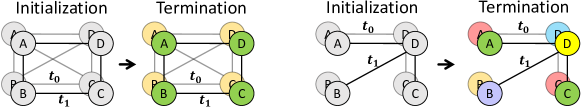
Figure 5: Two examples of temporal 1-WL test on non-attributive discrete-time dynamic graphs. The left test fails to distinguish non-isomorphic nodes at $t_{1}$, e.g., A and C, while the right example demonstrates a successful test.

Proposition 2.

If a discrete-time dynamic graph with a fixed graph topology at time $t$ has no repeated eigenvalues in its normalized graph Laplacian and has no missing frequency components in each snapshot, then the temporal 1-WL is able to differentiate all non-isomorphic nodes at time $t$.

We further prove that under the same assumptions, all pairs of nodes are non-isomorphic.

Proposition 3.

If a discrete-time dynamic graph with a fixed graph topology has no multiple eigenvalues in its normalized graph Laplacian and has no missing frequency components in each snapshot, then no automorphism exists.

Therefore, we close the gap and demonstrate that the expressive power of linear SPTGNNs is theoretically bounded by the proposed temporal 1-WL test.

3.3 Design of Spectral Filters

In this section, we outline a blueprint for designing powerful SPTGNNs, with all proofs available in Appendix C. We initially explore the optimal acquisition of spatial node embeddings within individual snapshots, focusing on the selection of the polynomial basis, $P_{k}(\cdot)$, for linear SPTGNNs.

Theorem 3.

For a linear SPTGNN optimized with mean squared loss, any complete polynomial bases result in the same expressive power, but an orthonormal basis guarantees the maximum convergence rate if its weight function matches the graph signal density.

This theorem guides the design of GSFs for learning node embeddings in each snapshot w.r.t. the optimization of coefficients. Following this, we discuss the optimal modeling of temporal clues between snapshots in spectral domains. We begin by analyzing the function bases in space projectors.

Lemma 1.

A time series with data points $x_{j}(t)$ can be expressed by $Q$ uncorrelated components $z_{i}(t)$ with an orthogonal (possibly complex) projector [16], i.e., $x_{j}(t)=\sum_{i=1}^{Q}e_{ij}z_{i}(t)$. The eigenvectors $e_{i}$ are orthogonal and determine the relationship between the data points $x_{j}(t)$.

Operating on all spectral components is normally unnecessary [17, 14]. Consider a multivariate time series $\mathbf{X}_{1}(t),\cdots,\mathbf{X}_{N}(t)$, where each $T$-length univariate time series $\mathbf{X}_{i}(t)$ is transformed into a vector $\mathbf{a}_{i}=({a}_{i,1},\cdots,{a}_{i,T})^{\top}\in\mathbb{R}^{T\times 1}$ through a space projection. We form matrix $\mathbf{A}=(\mathbf{a}_{1},\mathbf{a}_{2},\cdots,\mathbf{a}_{N})^{\top}\in\mathbb{R}^{N\times T}$ and apply a linear spectral filter as $\mathbf{A}\mathbf{W}$. Note that $\mathbf{A}$ does not denote the adjacency matrix here. We then randomly select $S<T$ columns in $\mathbf{A}$ using the masking matrix $\mathbf{S}\in\{0,1\}^{S\times T}$, obtaining compact representation $\mathbf{A}^{\prime}=\mathbf{A}\mathbf{S}^{\top}$ and linear spectral filtration as $\mathbf{A}^{\prime}\mathbf{W}$. We demonstrate that, under mild conditions, $\mathbf{A}^{\prime}\mathbf{W}$ preserves most information from $\mathbf{A}\mathbf{W}$. By projecting each column vector of $\mathbf{A}$ into the subspace spanned by column vectors in $\mathbf{A}^{\prime}$, we obtain $P_{\mathbf{A}^{\prime}}(\mathbf{A})=\mathbf{A}^{\prime}(\mathbf{A}^{\prime})^{\dagger}\mathbf{A}$. Let $\mathbf{A}_{k}$ represent $\mathbf{A}$’s approximation by its $k$ largest singular value decomposition. The lemma below shows $||\mathbf{A}\mathbf{W}-P_{\mathbf{A}^{\prime}}(\mathbf{A})\mathbf{W}||_{F}$ is close to $||\mathbf{W}||_{F}||\mathbf{A}-\mathbf{A}_{k}||_{F}$ if the number of randomly sampled columns $S$ is on the order of $k^{2}$.

Lemma 2.

Suppose the projection of $\mathbf{A}$ by $\mathbf{A}^{\prime}$ is $P_{\mathbf{A}^{\prime}}(\mathbf{A})$, and the coherence measure of $\mathbf{A}$ is $\mu(\mathbf{A})=\Omega(k/N)$, then with a high probability, the error between $\mathbf{A}\mathbf{W}$ and $P_{\mathbf{A}^{\prime}}(\mathbf{A})\mathbf{W}$ is bounded by $||\mathbf{A}\mathbf{W}-P_{\mathbf{A}^{\prime}}(\mathbf{A})\mathbf{W}||_{F}\leq(1+\epsilon)||\mathbf{W}||_{F}||\mathbf{A}-\mathbf{A}_{k}||_{F}$ if $S=O(k^{2}/\epsilon^{2})$.

The lemmas above demonstrate that in most cases we can express a 1-dimensional time series with (1) orthogonal space projectors and (2) a reduced-order linear spectral filter. For practical application on $D$-dimensional multivariate time series data, we simply extend dimensions in $\mathbf{S}$ and $\mathbf{W}$.

Theorem 4.

Assuming accurate node embeddings in each snapshot, a linear SPTGNN can, with high probability, produce expressive time series representations at valid times if its temporal FDMs consist of: (1) Linear orthogonal space projectors; (2) Individual reduced-order linear spectral filters.

3.4 Connection to Related Work

Here, we briefly discuss the connection between our theoretical framework and other GNN-based methods. See Appendix B for detailed related work. In comparison to MP-STGNNs, our approach offers two main advantages: (1) It can model differently signed time series relations by learning a wide range of GSFs (e.g., low-pass and high-pass); (2) On this basis, it can represent arbitrary multivariate time series under mild assumptions with provably expressive temporal FDMs. As such, our results effectively generalize these methods (Figure 2). While a few studies on SPTGNNs exist, e.g., StemGNN [7], our work is the first to establish a theoretical framework for generalizing this family of methods, which is strictly more powerful. See Appendix B for detailed comparisons.

4 Instantiation

In this section, we present a straightforward yet effective instantiation based on the discussion in section 3. We first outline the basic formulation of the proposed Temporal Graph GegenConv (TGC) and then connect it to other common practices. For the sake of clarity, we primarily present the canonical TGC, which contains only linear components in its building blocks and strictly inherits the basic formulation presented in Figure 3. Refer to Appendix D for model details. Again, our primary aim here is not to achieve state-of-the-art performance, but rather to validate our theoretical insights through the examination of TGC (and one of its variants, TGC^†).

Graph Convolution.

We implement $P_{k}(\cdot)$ in GSFs using the Gegenbauer basis due to its (1) generality and simplicity among orthogonal polynomials, (2) universality regarding its weight function, and (3) reduced model tuning expense. The Gegenbauer basis has the form $P_{k}^{\alpha}(x)=\frac{1}{k}[2x(k+\alpha-1)P_{k-1}^{\alpha}(x)-(k+2\alpha-2)P_{k-2}^{\alpha}(x)]$, with $P_{0}^{\alpha}(x)=1$ and $P_{1}^{\alpha}(x)=2\alpha x$ for $k<2$. Specifically, $P_{k}^{\alpha}(x),k=0,1,...$ are orthogonal on the interval $[-1,1]$ w.r.t. the weight function $(1-x^{2})^{\alpha-1/2}$. Based on this, we rewrite $P_{k}(\hat{\mathbf{L}})$ in Equation 2 as $P_{k}^{\alpha}(\mathbf{I}-\hat{\mathbf{L}})=P_{k}^{\alpha}(\hat{\mathbf{A}})$, and the corresponding graph frequency-domain model (convolution) is defined as $\sum_{k=0}^{K}\theta_{k}P^{\alpha}_{k}(\hat{\mathbf{A}})\mathbf{X}$.

Temporal Frequency-Domain Models.

When designing temporal FDMs, linear orthogonal projections should be approximately sparse to support dimension reduction, e.g., DFT. For spectral filters, we randomly select $S$ frequency components before filtration. Specifically, for components $\mathbf{f}\in\mathbb{C}^{T}$ in $\mathbf{F}\in\mathbb{C}^{N\times T\times D}$ along $N$ and $D$ dimensions, we denote sampled components as $\mathbf{f}^{\prime}:=\mathbf{f}_{\mathbb{I}}\in\mathbb{C}^{S}$, where $\mathbb{I}=\{i_{0},\cdots,i_{S-1}\}$ is a set of selection indices s.t. $\forall s\in\{0,\ldots,S-1\}$ and $i_{s-1}<i_{s}$. This is equivalent to $\mathbf{f}^{\prime}=\mathbf{f}\hat{\mathbf{S}}^{\top}$ with $\hat{\mathbf{S}}\in\{0,1\}^{S\times T}$, where $\hat{\mathbf{S}}_{i,s}=1$ if $i=i_{s}$. Thus, a standard reduced-order TSF is defined as $\mathbf{f}^{\prime}=\mathbf{f}\hat{\mathbf{S}}^{\top}\mathbf{W}$ with a trainable weight matrix $\mathbf{W}\in\mathbb{C}^{S\times S}$.

TGC Building Block.

Suppose $\tilde{\mathbf{Z}}=\sum_{k=0}^{K}\theta_{k}P^{\alpha}_{k}(\hat{\mathbf{A}})\mathbf{X}$, we discuss two linear toy temporal FDMs. We first consider a basic coarse-grained filtering with the masking and weight matrices $\mathbf{S}_{1}$ and $\mathbf{\Phi}_{1}$:

$$\mathbf{F} =\mathcal{F}(\tilde{\mathbf{Z}}), \hskip 5.0pt\mathbf{F}^{\prime} =\textsc{Pad}(\mathbf{F}\mathbf{S}_{1}^{\top}\mathbf{\Phi}_{1}), \hskip 5.0pt\mathbf{Z}^{\prime} =\mathcal{F}^{-1}(\mathbf{F}^{\prime}).$$ (3)

Next, we consider an optional fine-grained filtering based on time series decomposition, where $\mathbf{S}_{2}$ and $\mathbf{\Phi}_{2}$ are optimized to further capture the information in detailed signals (e.g., seasonalities) while maintaining global time series profiles (i.e., trends):

$$\mathbf{Z}^{\prime}_{t},\mathbf{Z}^{\prime}_{s} =\textsc{Decomp}(\mathbf{Z}^{\prime}), \hskip 3.00003pt\mathbf{F}_{s} =\mathcal{F}(\mathbf{Z}^{\prime}_{s}), \hskip 3.00003pt\mathbf{F}^{\prime}_{s} =\textsc{Pad}(\mathbf{F}_{s}\mathbf{S}_{2}^{\top}\mathbf{\Phi}_{2}), \hskip 3.00003pt\mathbf{Z} =\mathbf{Z}^{\prime}_{t}+\mathcal{F}^{-1}(\mathbf{F}^{\prime}_{s}).$$ (4)

After stacking multiple blocks, we forecast by transforming time series representations $\mathbf{Z}$. For time series decomposition and component padding, i.e., $\textsc{Decomp}(\cdot)$ and $\textsc{Pad}(\cdot)$, refer to Appendix D. In the same appendix, we also show that this implementation can be further boosted with the inclusion of nonlinearities and other common model choices (TGC^†), leading to more competitive performance.

Connection to Other Polynomial Bases.

We compare our design in TGC with other common practices in approximating graph convolutions: Monomial, Chebyshev, Bernstein, and Jacobi bases. More details are in Appendix E. For non-orthogonal polynomials, such as Monomial and Bernstein, our method with the Gegenbauer basis guarantees faster model convergences (Theorem 3) and better empirical performances in most cases. Compared with other orthogonal polynomials, we know that: (1) Our basis is a generalization of the second-kind Chebyshev basis; (2) Though our choice is a particular form of the Jacobi basis, the orthogonality of the Gegenbauer basis is well-posed in most real-world scenarios concerning its weight function; thus, our design is a simpler and nearly optimal solution for our purpose with only minor performance degradation.

5 Experiment

In this section, we evaluate the effectiveness and efficiency of our method on seven real-world benchmarks by comparing TGC and TGC^† with twenty different baselines. To empirically validate our theoretical claims, we further perform extensive ablation studies and present a variety of visualizations using both synthetic and real-world examples.

Table 1: Short-term forecasting results on four traffic benchmarks. We use the bold and underline fonts to indicate the best and second-best results. We follow [7] and [18] for the experimental setting and baseline results in left and right tables, respectively.

Method	MAE	RMSE	MAE	RMSE	MAE	RMSE	MAE	RMSE
	PeMS03		PeMS04		PeMS07		PeMS08
LSTNet [19]	19.07	29.67	24.04	37.38	2.34	4.26	20.26	31.69
DeepState [20]	15.59	20.21	26.50	33.00	3.95	6.49	19.34	27.18
DeepGLO [21]	17.25	23.25	25.45	35.90	3.01	5.25	15.12	25.22
DCRNN [22]	18.18	30.31	24.70	38.12	2.25	4.04	17.86	27.83
STGCN [2]	17.49	30.12	22.70	35.50	2.25	4.04	18.02	27.83
GWNet [3]	19.85	32.94	26.85	39.70	-	-	19.13	28.16
StemGNN [7]	14.32	21.64	20.24	32.15	2.14	4.01	15.83	24.93
TGC (Ours)	13.52	21.74	18.77	29.92	1.92	3.35	14.55	22.73

Method	MAE	RMSE	MAE	RMSE	MAE	RMSE	MAE	RMSE
	PeMS03		PeMS04		PeMS07		PeMS08
ASTGCN [23]	17.34	29.56	22.93	35.22	3.14	6.18	18.25	28.06
MSTGCN [23]	19.54	31.93	23.96	37.21	3.54	6.14	19.00	29.15
STG2Seq [24]	19.03	29.83	25.20	38.48	3.48	6.51	20.17	30.71
LSGCN [25]	17.94	29.85	21.53	33.86	3.05	5.98	17.73	26.76
STSGCN [26]	17.48	29.21	21.19	33.65	3.01	5.93	17.13	26.80
STFGNN [27]	16.77	28.34	20.48	32.51	2.90	5.79	16.94	26.25
STGODE [28]	16.50	27.84	20.84	32.82	2.97	5.66	16.81	25.97
TGC† (Ours)	16.22	27.07	20.00	32.10	2.81	5.58	16.54	26.10

Table 2: Long-term forecasting results on three time series benchmarks. We follow [29] for the experimental setting and baseline results. We use same notations as in Table 1.

Method		TGC†		FiLM [29]		FEDformer [14]		Autoformer [30]		Informer [31]		LogTrans [32]		Reformer [33]
Metric		MAE	RMSE	MAE	RMSE	MAE	RMSE	MAE	RMSE	MAE	RMSE	MAE	RMSE	MAE	RMSE
Electricity	96	0.293	0.425	0.267	0.392	0.297	0.427	0.317	0.448	0.368	0.523	0.357	0.507	0.402	0.558
	192	0.303	0.440	0.258	0.404	0.308	0.442	0.334	0.471	0.386	0.544	0.368	0.515	0.433	0.590
	336	0.313	0.470	0.283	0.433	0.313	0.460	0.338	0.480	0.394	0.548	0.380	0.529	0.433	0.591
Weather	96	0.235	0.408	0.262	0.446	0.296	0.465	0.336	0.515	0.384	0.547	0.490	0.677	0.596	0.830
	192	0.286	0.468	0.288	0.478	0.336	0.525	0.367	0.554	0.544	0.773	0.589	0.811	0.638	0.867
	336	0.317	0.515	0.323	0.516	0.380	0.582	0.395	0.599	0.523	0.760	0.652	0.892	0.596	0.799
Solar	96	0.242	0.443	0.311	0.557	0.363	0.448	0.552	0.787	0.264	0.469	0.262	0.467	0.255	0.451
	192	0.263	0.470	0.356	0.595	0.354	0.483	0.674	0.856	0.280	0.487	0.284	0.489	0.274	0.475
	336	0.271	0.478	0.370	0.628	0.372	0.518	0.937	1.131	0.285	0.496	0.295	0.512	0.278	0.491

Main Results.

Our method is evaluated against related work in terms of model effectiveness (Table 1 and Table 2, averaged over 5 runs) and efficiency (Table 3, averaged over 5 runs), showcasing the potential of SPTGNNs for time series forecasting. Our additional result statistics are in Appendix H. We compare our vanilla instantiation (TGC) with the most pertinent and representative works in Table 1 (left) on four traffic benchmarks, employing the forecasting protocol from [7]. Next, we assess our method (TGC^†, the nonlinear version of TGC) against state-of-the-art STGNNs in Table 1 (right), utilizing a standard testbed from [18]. Additionally, we report long-term forecasting results in Table 2, comparing our approach with state-of-the-art models and adhering to the setting in [29]. Detailed experimental setups are available in Appendix G.

Table 3: Efficiency comparison of representative models: Trainable parameters (M), time-per-epoch (s), and total training time (min); $\diamondsuit$ indicates significantly larger values compared to other methods.

Method	PeMS03	PeMS04	PeMS07	PeMS08
LSTNet	0.4/2.2/3.8	0.3/1.3/2.3	0.2/0.9/1.5	0.2/1.0/1.7
DeepGLO	0.6/14/8.3	0.6/8.5/6.0	0.3/6.2/6.6	0.3/5.9/4.2
DCRNN	OOM	0.4/$\diamondsuit$/$\diamondsuit$	0.4/$\diamondsuit$/$\diamondsuit$	0.4/$\diamondsuit$/$\diamondsuit$
STGCN	0.3/25/13	0.3/14/6.9	0.2/8.6/4.1	0.2/8.0/5.0
StemGNN	1.4/17/24	1.3/9.0/13	1.2/6.0/8.0	1.1/6.0/9.0
TGC	0.4/12/21	0.3/6.2/11	0.2/3.9/7.2	0.1/4.2/8.4

Our method consistently outperforms most baselines by significant margins in Table 1 and Table 2. In short-term forecasting, TGC and TGC^† achieve average performance gains of 7.3% and 1.7% w.r.t. the second-best results. Notably, we observe a significant improvement ($\sim$8%) over StemGNN [7], a special case of our method with nonlinearities. Considerable enhancements are also evident when compared to ASTGCN [23] ($\sim$9%) and LSGCN [25] ($\sim$7%), which primarily differ from StemGNN in temporal dependency modeling and design nuances. In long-term forecasting, our method further exhibits impressive performance, outperforming the second-best results by about 3.3%. These results indicate that even simple, yet appropriately configured SPTGNNs (discussed in subsection 3.3) are potent time series predictors. In Table 3, we examine our method’s efficiency by comparing TGC to representative baselines. We find that TGC forms the simplest and most efficient SPTGNN to date compared with StemGNN. In comparison to other STGNNs, such as STGCN [2] and DCRNN [22], our method also exhibits superior model efficiency across various aspects. Though deep time series models like LSTNet [19] are faster in model training, they do not have spatial modules and thus less effective.

Evaluation of Modeling Time Series Dependencies.

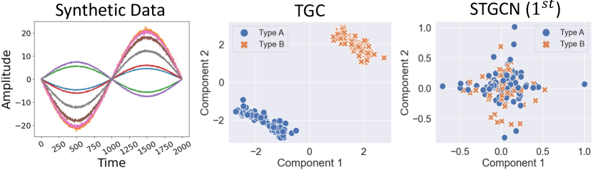
(a) Visualization of learned embeddings w.r.t. different time series correlations on a synthetic dataset. Types A and B represent series groups with opposing trends.

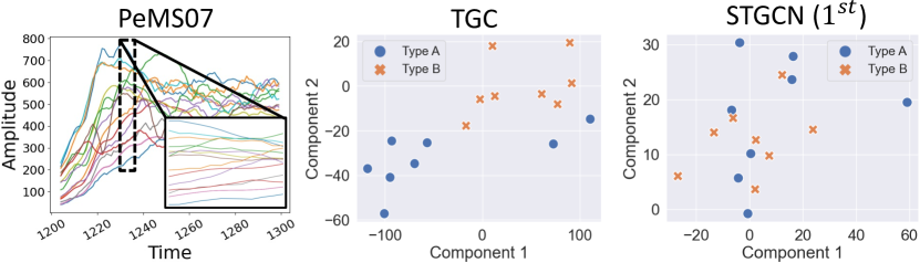
(b) Visualization of learned embeddings w.r.t. different time series correlations on PeMS07 dataset. Types A and B represent series groups with opposing trends.

Figure 6: Evaluation of learning differently signed time series relations.

Our method, in contrast to most GNN-based approaches, excels at learning different signed spatial relations between time series. Predetermined or learned graph topologies typically reflect the strength of underlying connectivity, yet strongly correlated time series might exhibit distinct properties (e.g., trends), which MP-STGNNs often struggle to model effectively. To substantiate our claims, we first visualize and compare the learned TGC and STGCN$(1^{st})$ [2] representations on two synthetic time series groups with positive and negative correlations. 6(a) reveals that STGCN$(1^{st})$ fails to differentiate between the two correlation groups. This is because methods like STGCN$(1^{st})$ aggregate neighborhood information with a single perspective (i.e., low-pass filtration). We further examine the learned embeddings of two groups of randomly sampled time series between TGC and STGCN$(1^{st})$ on a real-world traffic dataset (6(b)), where similar phenomena can be observed. Our experimental settings are detailed in Appendix G.

Ablation Studies.

Table 4: Ablation study results. We use the bold and underline fonts to denote the best and second-best results in each ablation block, respectively.

Variant	MAE	RMSE	MAE	RMSE	MAE	RMSE	MAE	RMSE
	PeMS03		PeMS04		PeMS07		PeMS08
A.1 Monomial	27.64	43.52	59.41	120.18	5.68	8.73	29.36	43.37
A.2 Bernstein	27.38	43.17	55.17	105.13	5.57	8.64	27.57	40.28
A.3 Chebyshev	13.56	21.84	18.78	29.89	1.94	3.37	14.36	22.93
A.4 Gegenbauer	13.52	21.74	18.77	29.92	1.92	3.35	14.35	22.73
A.5 Jacobi	13.14	21.51	18.64	29.44	1.91	3.34	14.29	22.15
TGC (Ours)	13.52	21.74	18.77	29.92	1.92	3.35	14.55	22.73
B.1 w/o MD-F	14.07	21.82	19.07	30.34	2.05	3.45	15.14	23.49
B.2 w/o MD-F†	13.62	21.73	18.92	30.11	1.96	3.40	15.06	23.25
B.3 w/o MV-F	13.80	21.77	19.12	30.50	1.97	3.44	15.12	23.58
B.4 w/o O-SP	13.72	21.75	19.10	30.42	2.03	3.53	15.38	28.84
B.5 w/o C-FDM	13.83	21.47	19.15	30.52	2.01	3.47	15.18	23.71
B.6 w/o F-FDM	13.71	21.59	18.81	29.96	1.93	3.39	14.88	23.10
TGC† (Ours)	13.39	21.34	18.41	29.39	1.84	3.28	14.38	22.43
C.1 w/o NL	13.75	21.43	18.63	29.70	1.92	3.36	14.94	24.93
C.2 w/o S-Attn	13.42	21.38	18.50	29.53	1.86	3.30	14.43	22.54

We perform ablation studies from three perspectives. First, we evaluate the GSFs in TGC with different polynomial bases (A.1 to A.5) in the first block. Next, we examine other core designs in the second block: B.1 and B.2 apply identical polynomial coefficients in GSFs and trainable weights in temporal FDMs along $D$ dimensions, respectively. B.3 utilizes the same set of TSFs across $N$ variables. B.4 replaces orthogonal space projections with random transformations. B.5 and B.6 separately remove the coarse-grained and fine-grained temporal FDMs. Lastly, we evaluate add-ons that make TGC^†. C.1 eliminates nonlinearities, and C.2 disables the spectral attention.

In the first block of results, we validate the discussion in section 4: (1) Orthogonal polynomials (A.3 to A.5) yield significantly better performance than non-orthogonal alternatives (A.1 and A.2); (2) Although the performance gaps between A.3 to A.5 are minor, polynomial bases with orthogonality that hold on more general weight functions tend to result in better performances. The results of B.1 to B.3 support the analysis of multidimensional and multivariate predictions in subsection 3.2, with various degradations observed. In B.4, we see an average 4% MAE and 7% RMSE reduction, confirming the related analysis in subsection 3.3. The results of B.5 and B.6 indicate that both implementations (Equation 3 and Equation 4) are effective, with fine-grained temporal FDMs icing on the cake. In the last block, we note a maximum 3.1% and 0.8% improvement over TGC by introducing nonlinearities (C.2) and spectral attention (C.1). Simply combining both leads to even better performance (i.e., TGC^†).

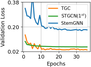
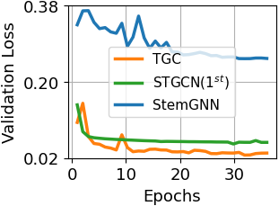
Figure 7: Model convergence comparison on PeMS07 dataset. Left: $lr=0.01$. Right: $lr=0.001$.

Model Convergence.

We compare model convergence between STGCN$(1^{st})$ [2], StemGNN [7], and TGC across two scenarios with different learning rates. Our instantiation with Gegenbauer bases has the fastest convergence rate in both cases, further confirming Theorem 3 with ablation studies. Also, as anticipated, STGCN$(1^{st})$ is more tractable than StemGNN w.r.t. the model training due to certain relaxations but at the cost of model effectiveness.

Additional Experiments.

Refer to Appendix H for details. (1) We evaluate TGC against additional baselines on other time series benchmarks; (2) We conduct parameter studies examining the impact of the Gegenbauer parameter $\alpha$, polynomial degree $K$, number of selected modes $S$, and number of building blocks $M$; (3) Additional visualizations; (4) Statistics of our results in Table 1 and Table 2.

6 Conclusion

We formally define spectral-temporal GNNs and establish a theoretical framework for this family of methods, with the following important takeaways: (1) Spectral-temporal GNNs can be universal with mild assumptions; (2) Orthogonal bases and individual spectral filters are key to designing powerful GNN-based time series models. To validate our theorem, we propose a simple instantiation (TGC) and its nonlinear variant (TGC^†), outperforming most baselines on various real-world benchmarks.

Having established a firm theoretical groundwork for GNN-based time series forecasting, we are yet to explore specific scenarios such as time-evolving graph structures. Additionally, investigating the applicability of our theories to other tasks, such as time series classification and anomaly detection, would also be valuable. We leave these explorations for future work.

Appendix A Preliminaries

For a matrix $\mathbf{M}\in\mathbb{R}^{a\times b}$, we denote $\mathbf{M}_{i,:}$ and $\mathbf{M}_{:,j}$ as the $i^{\text{th}}$ row and $j^{\text{th}}$ column of this matrix. Specifically, we use $\mathbf{M}_{\mathbb{A}\mathbb{B}}$ to denote a submatrix of $\mathbf{M}$ with row and column index sets $\mathbb{A}$ and $\mathbb{B}$. Suppose $\mathbf{M}$ can be factorized into a canonical form and represented by its eigenvalues $\mathbf{\Lambda}$ and eigenvectors $\mathbf{U}$, we denote its condition number as $\kappa{(\mathbf{M})}=\frac{|\lambda_{max}|}{|\lambda_{min}|}$, where $\lambda_{min}$ and $\lambda_{max}$ are the smallest and largest eigenvalues, respectively. $\kappa{(\mathbf{M})}=\infty$ if $\mathbf{M}$ is singular.

A.1 Graph Spectral Filtering

In this work, we model a multivariate time series with the length $T$ as a set of undirected graph snapshots $\{\mathcal{G}_{t}\}^{T-1}_{t=0}$ s.t. $\mathcal{G}_{t}=(\mathbf{A},\mathbf{X}_{t})$. Given a graph topology $\mathbf{A}$, we have its degree matrix defined as $\mathbf{D}\in\mathbb{R}^{N\times N}$ s.t. $\mathbf{D}_{i,i}=\sum_{j=1}^{N}\mathbf{A}_{i,j}$, which is symmetric. On this basis, we define the normalized graph Laplacian matrix as $\hat{\mathbf{L}}=\mathbf{D}^{-\frac{1}{2}}\mathbf{L}\mathbf{D}^{-\frac{1}{2}}$, where $\mathbf{L}=\mathbf{D}-\mathbf{A}$, and we know $\hat{\mathbf{L}}$ is symmetric and positive semi-definite. We let its eigendecomposition of $\hat{\mathbf{L}}$ to be $\hat{\mathbf{L}}=\mathbf{U}\mathbf{\Lambda}\mathbf{U}^{\top}$, where $\mathbf{\Lambda}$ and $\mathbf{U}$ are matrices of eigenvalues and eigenvectors. We first define graph Fourier transformation (GFT) below.

Definition A1.

Graph Fourier transform of the signal $\mathbf{X}_{t}$ is defined as $\tilde{\mathbf{X}}_{t}=\mathbf{U}^{\top}\mathbf{X}_{t}$, where $\tilde{\mathbf{X}}_{t}^{(\lambda)}=\mathbf{U}^{\top}_{:,\lambda}\mathbf{X}_{t}$ denote the frequency component of input signal at the frequency $\lambda$. Corresponsively, the inverse graph Fourier transform of $\tilde{\mathbf{X}}_{t}$ is defined as $\mathbf{X}_{t}=\mathbf{U}\tilde{\mathbf{X}}_{t}$.

The above definition describes how to transform input signals between original and orthonormal spaces, and we say $\mathbf{X}_{t}$ contains $\lambda$ frequency component if $\tilde{\mathbf{X}}_{t}^{(\lambda)}\neq\vec{0}$. To filter input signals in the frequency domain w.r.t. node connectivity, we have graph convolution defined below.

Definition A2.

Assume there is a filter function of eigenvalues $g(\cdot):[0,2]\mapsto\mathbb{R}$, we define the spectral convolution on $\mathcal{G}_{t}$ as filtering the input signal $\mathbf{X}_{t}$ with the spectral filter:

$$g(\mathbf{\Lambda})\star\mathbf{X}_{t}:=\mathbf{U}g(\mathbf{\Lambda})\mathbf{U}^{\top}\mathbf{X}_{t}.$$ (S1)

The filter function can be parameterized, i.e., $g_{\theta}(\mathbf{\Lambda})$, but directly calculating the above equation requires eigendecomposition with the time complexity of $\mathcal{O}(N^{3})$. To alleviate this issue, we can first approximate $g_{\theta}(\mathbf{\Lambda})$ with a truncated expansion of a polynomial with $K$ degrees:

$$g_{\theta}(\lambda):=\sum_{k=0}^{K}\mathbf{\Theta}_{k,:}P_{k}(\lambda).$$ (S2)

Thus, graph spectral filtering takes the following form:

$$\small\mathbf{U}g_{\theta}(\mathbf{\Lambda})\mathbf{U}^{\top}\mathbf{X}_{t}:=\sum_{k=0}^{K}\mathbf{\Theta}_{k,:}\mathbf{U}P_{k}(\mathbf{\Lambda})\mathbf{U}^{\top}\mathbf{X}_{t}=\sum_{k=0}^{K}\mathbf{\Theta}_{k,:}P_{k}(\hat{\mathbf{L}})\mathbf{X}_{t}.$$ (S3)

If we let $g_{\theta}(\hat{\mathbf{L}})=\sum_{k=0}^{K}\mathbf{\Theta}_{k,:}P_{k}(\hat{\mathbf{L}})$, we derive the following practical spectral graph convolution operation that goes beyond the low-pass filtering:

$$g(\mathbf{\Lambda})\star\mathbf{X}_{t}:=g_{\theta}(\hat{\mathbf{L}})\mathbf{X}_{t}.$$ (S4)

A.2 Orthogonal Time Series Representations

In real-world time series data, complex behaviors such as periodic patterns are prevalent. Spectral analysis facilitates the disentanglement and identification of these patterns. This study aims to represent time series using sparse orthogonal components. Given an input signal, $\mathbf{X}_{n}$, its values at time $t$ are denoted as $\mathbf{X}_{n}(t)$. As per Lemma 1, numerous orthogonal projections, such as discrete Fourier or cosine transformations, can serve as space projections for our objectives.

Definition A3.

Discrete Fourier transformation (DFT) on time series takes measurements at discrete intervals, and transforms observations into frequency-dependent amplitudes:

$$\small\tilde{\mathbf{X}}_{n}(k)=\sum_{t=0}^{T-1}\mathbf{X}_{n}(t)e^{-2\pi ikt/T},\ k=\{0,1,\cdots,T-1\}.$$ (S5)

Inverse transformation (IDFT) maps a signal from the frequency domain back to the time domain:

$$\small\mathbf{X}_{n}(t)=\frac{1}{T}\sum_{k=0}^{T-1}\tilde{\mathbf{X}}_{n}(k)e^{2\pi ikt/T},\ t=\{0,1,\cdots,T-1\}.$$ (S6)

Definition A4.

Discrete cosine transformation (DCT) is similar but uses real numbers, which express a sequence of observations with a set of cosine waves oscillating at different frequencies:

$$\small\tilde{\mathbf{X}}_{n}(k)=\sqrt{\frac{2}{T}}\sum_{t=0}^{T-1}\mathbf{X}_{n}(t)\text{cos}\big{[}\frac{\pi}{T}(t+\frac{1}{2})(k+\frac{1}{2})\big{]},\ k=\{0,1,\cdots,T-1\}.$$ (S7)

Inverse transformation (IDCT) distributes the data back to the time domain by multiplying $2/T$.

In this study, we employ DFT and IDFT by default in temporal frequency-domain models.

Appendix B Related Work

B.1 Deep Time Series Forecasting

Time series forecasting has been extensively researched over time. Traditional approaches primarily focus on statistical models, such as vector autoregressive (VAR) lutkepohl2013vector and autoregressive integrated moving average (ARIMA) box2015time. In contrast, deep learning-based methods have recently achieved significant success. Deep learning-based approaches, on the other hand, have achieved great success in recent years. For example, recurrent neural network (RNN) and its variants, e.g., FC-LSTM shi2015convolutional, are capable to well model univariate time series. TCN bai2018empirical improves these methods by modeling multivariate time series as a unified entity and considering the dependencies between different variables. Follow-up research, such as LSTNet [19] and DeepState [20], proposes more complex models to handle interlaced temporal and spatial clues by marrying sequential models with convolution networks or state space models. Recently, Transformer vaswani2017attention-based approaches have made great leaps, especially in long-term forecasting wen2022transformers. For these methods, an encoder-decoder architecture is normally applied with improved self- and cross-attention, e.g., logsparse attention [32], locality-sensitive hashing [33], and probability sparse attention [31]. As time series can be viewed as a signal of mixed seasonalities, Zhou et al. further propose FEDformer [14] and a follow-up work FiLM [29] to rethink how spectral analysis benefits time series forecasting. Nevertheless, these methods do not explicitly model inter-time series relationships (i.e., spatial dependencies), and we elaborate on the connections between them and our research later in this section.

B.2 Spatial-Temporal Graph Neural Networks

A line of research explores capturing time series relations using GNNs. For instance, DCRNN [22] combines recurrent units with graph diffusion [5] to simultaneously capture temporal and spatial dependencies, while Graph WaveNet [3] interleaves TCN bai2018empirical and graph diffusion layers. Subsequent studies, such as STSGCN [26], STFGNN [27], and STGODE [28], adopt similar principles but other ingenious designs to better characterize underlying spatial-temporal clues. However, these methods struggle to model differently signed time series relations since their graph convolutions operate under the umbrella of message passing, which serves as low-pass filtering assuming local homophiles. Some STGNNs, such as ASTGCN [23] and LSGCN [25], directly employ ChebConv [4] for capturing time series dependencies. However, their graph convolutions using the Chebyshev basis, along with the intuitive temporal models they utilize, result in sub-optimal solutions. Consequently, the expressiveness of most STGNNs remains limited. Spectral-temporal graph neural networks (SPTGNNs), on the other hand, first make it possible to fill the gap by (properly) approximating both graph and temporal convolutions with a broad range of filters in spectral domains, allowing for better pattern extraction and modeling. A representative work in this category is StemGNN [7]. However, it faces two fundamental limitations: (1) Its direct application of ChebConv is sub-optimal, and (2) although its temporal FDMs employ orthogonal space projections, they fail to make proper multidimensional and multivariate predictions as discussed. We elaborate on the connection between our research and GNN-based time series forecasting methods later in this section.

B.3 Spectral Graph Neural Networks

Spectral graph neural networks are grounded in spectral graph signal filtering, where graph convolutions are approximated by truncated polynomials with finite degrees. These graph spectral filters can be either trainable or not. Examples with predefined spectral filters include APPNP gasteiger2018predict and GraphHeat xu2019graph, as illustrated in [8]. Another branch of work employs different polynomials with trainable coefficients (i.e., filter weights) to approximate effective graph convolutions. For instance, ChebConv [4] utilizes Chebyshev polynomials, inspiring the development of many popular spatial GNNs with simplifications kipf2016semiluo2023npfkgc. BernNet [8] employs Bernstein polynomials but can only express positive filter functions due to regularization constraints. Recently, JacobiConv [13] demonstrated that graph spectral filtering with Jacobi polynomial approximation is highly effective on a wide range of graphs under mild constraints. Although spectral graph neural networks pave the way for SPTGNNs, they primarily focus on modeling static graph-structured data without the knowledge telling how to effectively convolute on dynamic graphs for modeling time series data.

B.4 Connection to Related Work

We discuss the connection between our theoretical framework of SPTGNNs and most related works, including deep time series models, spatial-temporal GNNs, and spectral GNNs. Most of the deep time series models approximate expressive temporal filters with deep neural networks and learn important patterns directly in the time domain, e.g., TCN bai2018empirical, where some complex properties (e.g., periodicity) may not be well modeled. Our work generalizes these methods in two ways: (1) When learning on univariate time series data, our temporal frequency-domain models guarantee that the most significant properties are well modeled with high probability (Lemma 1 and Lemma 2); (2) When learning on multivariate time series data, our framework models diverse inter-relations between time series (Figure 1) and intra-relations within time series with theoretical evidence. For most spatial-temporal GNNs, they either use the first-order approximation of ChebyConv [4] (e.g., STGCN$(1^{st})$ [2]) or graph diffusion (e.g., DCRNN [22]) to model time series dependencies. These methods can be generalized as message-passing-based spatial-temporal GNNs (MP-STGNNs). In comparison, our framework has two major advantages: (1) It can model differently signed time series relations by learning a wide range of graph spectral filters (e.g., low-pass and high-pass), while MP-STGNNs only capture positive correlations between time series exhibiting strong similarities; (2) On this basis, it can express any multivariate time series under mild assumptions with provably expressive temporal frequency-domain models, while MP-STGNNs approximate effective temporal filtering in time domains with deep neural networks. Even compared to STGNNs employing ChebyConv, our proposal generalizes them well: (1) We provide a blueprint for designing effective graph spectral filters and point out that using Chebyshev basis is sub-optimal; (2) Instead of approximating expressive temporal models with deep neural networks, we detail how to simply construct them in frequency domains. Therefore, our results generalize most STGNNs effectively. Although there are few studies on SPTGNNs, such as StemGNN [7], we are not only the first to define the general formulation and provide a theoretical framework to generalize this branch of methods but also free from the limitations of StemGNN mentioned above. Compared with spectral GNNs, such as BernNet [8] and JacobiConv [13], our work extends graph convolution to model dynamic graphs comprising a sequence of regularly-sampled graph snapshots. A detailed comparison between the polynomial basis in our instantiation and that in common spectral GNNs is in Appendix E.

Appendix C Proofs

C.1 Proof of Theorem 1

Theorem 1. A linear SPTGNN can produce arbitrary dimensional time series representations at any valid time iff: (1) $\hat{\mathbf{L}}$ has no repeated eigenvalues; (2) $\mathbf{X}$ encompasses all frequency components with respect to the graph spectrum; (3) $\mathcal{T}_{\phi}(\cdot)$ can express any single-dimensional univariate time series.

Proof.

Let us assume that $t=1$ (i.e., there is only one snapshot $\mathcal{G}_{t}$ of the graph $\{\mathcal{G}_{t}\}_{t=0}^{T-1}$), $\mathcal{T}_{\phi}(\cdot)$ reduces to linear functions of a graph snapshot and the linear spectral-temporal GNN reduces to a linear spectral GNN, which can be equivalently written as:

$$\mathbf{Z}_{t}=g_{\theta}(\hat{\mathbf{L}})\mathbf{X}_{t}\mathbf{\Phi}\in\mathbb{R}^{N\times D}.$$ (S8)

We first prove the universality theorem of linear spectral GNNs in a graph snapshot on the basis of Theorem 4.1 in [13]. In other words, assuming $\tilde{\mathbf{X}}_{t}=\mathbf{U}^{\top}\mathbf{X}_{t}$ has non-zero row vectors and $\hat{\mathbf{L}}$ has unique eigenvalues, we first aim to prove that for any $\mathbf{Z}_{t,d}\in\mathbb{R}^{N\times 1}$, there is a linear spectral GNN to produce it. We assume there exists $\boldsymbol{\phi}^{*}\in\mathbb{R}^{D}$ s.t. all elements in $\tilde{\mathbf{X}}_{t}\boldsymbol{\phi}^{*}$ are non-zero. Considering a case where $(\tilde{\mathbf{X}}_{t}\boldsymbol{\phi})_{i}=0$ and letting the solution space to be $\mathbb{S}_{i}$, we know that $\mathbb{S}_{i}$ is a proper subspace of $\mathbb{R}^{D}$ as the $i$-th row of $\tilde{\mathbf{X}}_{t}$ is non-zero. Therefore, $\mathbb{R}^{D}\setminus\cup_{i=1}^{N}\mathbb{S}_{i}\neq\emptyset$, and we know that all vectors $\boldsymbol{\phi}$ in $\mathbb{R}^{D}\setminus\cup_{i=1}^{N}\mathbb{S}_{i}$ are valid to form $\boldsymbol{\phi}^{*}$. We then filter $\tilde{\mathbf{X}}_{t}\boldsymbol{\phi}^{*}$ to get $\mathbf{Z}_{t,d}$. Firstly, we let $\tilde{\mathbf{Z}}_{t,d}=\mathbf{U}^{\top}\mathbf{Z}_{t,d}$ and assume there is a polynomial with $N-1$ order:

$$p_{i} :=g_{\theta}(\lambda_{i}),$$ (S9)

$$=\sum_{k=0}^{N-1}\theta_{k}\lambda_{i}^{k}\ \ \ \text{s.t.}\ \ \ p_{i}=\tilde{\mathbf{Z}}_{t,d}[i]/(\tilde{\mathbf{X}}_{t}\boldsymbol{\phi}^{*})_{i}\ \ \ \text{and}\ \ \ \forall i\in\{1,\cdots,N\}.$$

On this basis, the polynomial coefficients $\boldsymbol{\theta}$ is the solution of a linear system $\mathbf{B}\boldsymbol{\theta}=\mathbf{p}$ where $\mathbf{B}_{i,j}=\lambda_{i}^{j-1}$. Since $\lambda_{i}$ are different from each other, $\mathbf{B}^{\top}$ turns to a nonsingular Vandermonde matrix, where a solution $\boldsymbol{\theta}$ always exists. Therefore, a linear spectral GNN can produce any one-dimensional prediction under certain assumptions.

The above proof states that linear spectral GNNs can produce any one-dimensional prediction if $\hat{\mathbf{L}}$ has no repeated eigenvalues (i.e., condition 1) and the node features $\mathbf{X}$ contain all frequency components w.r.t. graph spectrum (i.e., condition 2). When $t\geq 2$, $\mathcal{T}_{\phi}(\cdot)$ turns to linear functions over all historical observations of graph snapshots. In order to distinguish between different historical graph snapshots, $\mathcal{T}_{\phi}(\cdot)$ must be universal approximations of all historical graph snapshots, implying that $\mathcal{T}_{\phi}(\cdot)$ is able to express any one-dimensional univariate time series (i.e., condition 3). ∎

C.2 Proof of Theorem 2

Theorem 2. For a linear SPTGNN with valid temporal FDMs and a $K$-degree polynomial basis in its GSFs, $\forall u,v\in\mathbb{V},\mathbf{Z}_{t}[u]=\mathbf{Z}_{t}[v]$ if $\mathbf{C}^{(K+1)}(u,t)=\mathbf{C}^{(K+1)}(v,t)$. $\mathbf{Z}_{t}[i]$ and $\mathbf{C}^{(K)}(i,t)$ represent node $i$’s embedding at time $t$ in such a GNN and the $K$-step temporal 1-WL test, respectively.

Proof.

Given valid temporal frequency-domain models (i.e., space projectors and TSFs) and a $K$-degree polynomial filter function, the prediction of a linear SPTGNN can be formulated as follows.

$$\mathbf{Z}=\mathcal{T}_{\phi}\left(\sum_{k=0}^{K}\boldsymbol{\Theta}_{k}P_{k}(\hat{\mathbf{L}})\mathbf{X}\right).$$ (S10)

For ease of reading, we redefine $\mathcal{T}_{\phi}(\cdot)$ as the combination of space projections and TSFs in the following proof. Let us assume $t=1$ (i.e., there is only one snapshot $\mathcal{G}_{t}$ of the graph $\{\mathcal{G}_{t}\}_{t=0}^{T-1}$), $\mathcal{T}_{\phi}(\cdot)$ reduces to linear functions of a single graph snapshot and a linear SPTGNN reduces to a linear spectral GNN. Using the framework in xu2019graph, Equation S10 can be viewed as a $k+1$-layer GNN. The output of the last layer in GNN produces the output of linear spectral GNNs [13]. According to the proof of Lemma 2 in xu2019graph, if WL node labels $\mathbf{C}^{(K+1)}(u)=\mathbf{C}^{(K+1)}(v)$, the corresponding GNN’s node features should be the same at any iteration. Therefore, for all nodes $\forall u,v\in\mathbb{V},\mathbf{Z}[u]=\mathbf{Z}[v]$ if $\mathbf{C}^{(K+1)}(u)=\mathbf{C}^{(K+1)}(v)$.

When $t\geq 2$, we have a DTDG defined as a sequence of graph snapshots $\left(\mathcal{G}_{1},\mathcal{G}_{2},\ldots\right)$ that are sampled at regular intervals, and each snapshot is a static graph. Note that any DTDGs can be equivalently converted to continuous-time temporal graphs (CTDGs). The CTDG can be equivalently viewed as time-stamped multi-graphs with timestamped edges, i.e., $\mathcal{G}(t)=$ $\left\{\left(u_{k},v_{k},t_{k}\right)\mid t_{k}<t\right\}$. According to Proposition 6 in [15], the expressive power of dynamic GNN with injective message passing is bounded by the temporal WL test on $\mathcal{G}(t)$. Since $\mathcal{T}_{\phi}(\cdot)$ is a set of linear functions over all historical observations of graph snapshots, i.e., $\mathcal{T}_{\phi}(\cdot)$ represents linear transformations of $\mathcal{G}(t)$. The defined SPTGNN, i.e., $\mathbf{Z}=\mathcal{T}_{\phi}(\sum_{k=0}^{K}\boldsymbol{\Theta}_{k}P_{k}(\hat{\mathbf{L}})\mathbf{X})$, should be as expressive as dynamic GNN with injective message passing. Hence, if temporal WL node labels $\mathbf{C}^{(K+1)}(u,t)=\mathbf{C}^{(K+1)}(v,t)$, the corresponding GNN’s node features should be the same at any timestamp $t$ and at any iteration. Therefore, for all nodes $\forall u,v\in\mathbb{V},\mathbf{Z}_{t}[u]=\mathbf{Z}_{t}[v]$ if $\mathbf{C}^{(K+1)}(u,t)=\mathbf{C}^{(K+1)}(v,t)$. ∎

C.3 Proof of Proposition 2

Proposition 2. If a discrete-time dynamic graph with a fixed graph topology at time $t$ has no repeated eigenvalues in its normalized graph Laplacian and has no missing frequency components in each snapshot, then the temporal 1-WL is able to differentiate all non-isomorphic nodes at time $t$.

Proof.

Assume there are no repeated eigenvalues and missing frequency components w.r.t. graph spectrum in a DTDG with fixed topology and time-evolving features, i.e., $\{\mathcal{G}_{t}\}_{t=0}^{T-1}$.

According to Corollary 4.4 in [13], we know that if a graph has no repeated eigenvalues and missing frequency components, then 1-WL test can differentiate any pair of non-isomorphic nodes. We denote the colors of two nodes $u$ and $v$ in $\mathcal{G}_{t}$ after $L$ 1-WL interactions as $\mathbf{C}^{(L)}(u,t)$ and $\mathbf{C}^{(L)}(v,t)$ s.t. $\mathbf{C}^{(L)}(u,t)\neq\mathbf{C}^{(L)}(v,t)$ if $u$ and $v$ are non-isomorphic. On this basis, we consider two scenarios in $\mathcal{G}_{t+1}$: (1) Two or more non-isomorphic nodes have identical initial colors; (2) None of the non-isomorphic nodes have identical colors. Under the assumptions in this proposition, the 1-WL test can differentiate $u$ and $v$ in $\mathcal{G}_{t+1}$ on both cases with different

$\mathbf{C}^{(L)}(u,t+1):=\textsc{Hash}(c^{(L-1)}(u,t+1),\{\!\!\{c^{(L-1)}(m,t+1):e_{u,m,t+1}\in\mathbb{E}(\mathcal{G}_{t+1})\}\!\!\})$

and

$\mathbf{C}^{(L)}(v,t+1):=\textsc{Hash}(c^{(L-1)}(v,t+1),\{\!\!\{c^{(L-1)}(m,t+1):e_{v,m,t+1}\in\mathbb{E}(\mathcal{G}_{t+1})\}\!\!\})$.

Therefore, no matter whether $\mathbf{C}^{(L)}(u,t)$ and $\mathbf{C}^{(L)}(v,t)$ are identical or not (they are different in fact as mentioned), we have nonidentical

$\mathbf{C}^{(L)}(u,t+1):=\textsc{Hash}(c^{(L-1)}(u,t+1),c^{(L-1)}(u,t),\{\!\!\{c^{(L-1)}(m,t+1):e_{u,m,t+1}\in\mathbb{E}(\mathcal{G}_{t+1})\}\!\!\})$

and

$\mathbf{C}^{(L)}(v,t+1):=\textsc{Hash}(c^{(L-1)}(v,t+1),c^{(L-1)}(v,t),\{\!\!\{c^{(L-1)}(m,t+1):e_{v,m,t+1}\in\mathbb{E}(\mathcal{G}_{t+1})\}\!\!\})$ in the temporal 1-WL test, where $\mathbf{C}^{(L)}(u,t):=c^{(L-1)}(u,t)$ and $\mathbf{C}^{(L)}(v,t):=c^{(L-1)}(v,t)$. ∎

C.4 Proof of Proposition 3

Proposition 3. If a discrete-time dynamic graph with a fixed graph topology has no multiple eigenvalues in its normalized graph Laplacian and has no missing frequency components in each snapshot, then no automorphism exists.

Proof.

Given a DTDG $\{\mathcal{G}_{t}\}_{t=0}^{T-1}$ consists of $T$ static graph snapshots with fixed graph topology and time-evolving node features, we first prove that all pairs of nodes are non-isomorphic.

In a snapshot $\mathcal{G}_{t}$, assume there is a permutation matrix $\mathbf{P}$, we have

$$\hat{\mathbf{L}}:=\mathbf{P}^{\top}\hat{\mathbf{L}}\mathbf{P}=\mathbf{P}\mathbf{U}\mathbf{\Lambda}\mathbf{U}^{\top}\mathbf{P}^{\top},$$ (S11)

and we know

$$\mathbf{\Lambda}:=\mathbf{U}^{\top}\mathbf{P}\mathbf{U}\mathbf{\Lambda}\mathbf{U}^{\top}\mathbf{P}^{\top}\mathbf{U}=\mathbf{V}\mathbf{\Lambda}\mathbf{V}^{\top},$$ (S12)

where $\mathbf{V}$ is an orthogonal matrix. Since all diagonal elements in $\mathbf{\Lambda}$ are different because we assume no repeated eigenvalues, then the eigenspace of each eigenvalue has only one dimension [13]; thus, we have $\mathbf{U}^{\top}\mathbf{P}\mathbf{U}=\mathbf{D}$, where $\mathbf{D}$ is a diagonal matrix s.t. $\mathbf{V}:=\mathbf{D}$ with $\pm 1$ elements. Now considering the node features $\mathbf{X}_{t}:=\mathbf{P}\mathbf{X}_{t}$, we have $\hat{\mathbf{X}}_{t}=\mathbf{V}\hat{\mathbf{X}}_{t}$; thus $(\mathbf{I}-\mathbf{D})\hat{\mathbf{X}}_{t}=0$ based on the above discussion. If there are no missing frequency components in $\hat{\mathbf{X}}_{t}$, i.e., no zero row vectors, we have $\mathbf{D}=\mathbf{I}$ and know that

$$\mathbf{P}=\mathbf{U}\mathbf{D}\mathbf{U}^{\top}=\mathbf{I}.$$ (S13)

Hence, we prove that all nodes in a graph snapshot $\mathcal{G}_{t}$ are non-isomorphic. In $\{\mathcal{G}_{t}\}_{t=0}^{T-1}$, we have $\mathbf{V}:=\mathbf{D}$ always holds across all snapshots if its normalized graph Laplacian has no repeated eigenvalues. On this basis, if there are no missing frequency components by giving $\mathbf{X}_{t},\forall t\in\{0,1,\ldots,T-1\}$, all pairs of nodes are non-isomorphic in an attributed DTDG with fixed graph topology.

∎

C.5 Proof of Theorem 3

Theorem 3. For a linear SPTGNN optimized with mean squared loss, any complete polynomial bases result in the same expressive power, but an orthonormal basis guarantees the maximum convergence rate if its weight function matches the graph signal density.

Proof.

Directly analyzing Equation 2 is complex and unnecessary to study the effectiveness of different polynomial bases when learning time series relations at each time step. Since optimizing the spectral-temporal GNNs formulated in Equation 2 can be understood as a two-step (i.e., graph-then-temporal) optimization problem, we directly analyze the optimization of $\mathbf{\Theta}$ w.r.t. the formulation below based on the squared loss $\mathcal{L}=\frac{1}{2}||\mathbf{Z}_{t}-\mathbf{Y}_{t}||^{2}_{F}$ on a graph snapshot $\mathcal{G}_{t}$ with the target $\mathbf{Y}_{t}$.

$$\mathbf{Z}_{t}=\sum_{k=0}^{K}\mathbf{\Theta}_{k}P_{k}(\hat{\mathbf{L}})\mathbf{X}_{t}.$$ (S14)

This is a convex optimization problem, thus the convergence rate of gradient descent relates to the condition number of the Hessian matrix boyd2004convex. In other words, the convergence rate reaches the maximum if $\kappa{(\mathbf{H})}$ reaches the minimum. We have $\mathbf{H}_{k_{1},k_{2}}$ defined as follows that is similar in [13].

$$\frac{\partial\mathcal{L}}{\partial\mathbf{\Theta}_{k_{1}}\partial\mathbf{\Theta}_{k_{2}}} =\mathbf{X}_{t}^{\top}P_{k_{2}}(\hat{\mathbf{L}})P_{k_{1}}(\hat{\mathbf{L}})\mathbf{X}_{t},$$ (S15)

$$=\sum_{i=1}^{n}P_{k_{2}}(\lambda_{i})P_{k_{1}}(\lambda_{i})\tilde{\mathbf{X}}_{t}[\lambda_{i}].$$

This equation can be written as a Riemann sum as follows.

$$\frac{\partial\mathcal{L}}{\partial\mathbf{\Theta}_{k_{1}}\partial\mathbf{\Theta}_{k_{2}}}=\sum_{i=1}^{n}P_{k_{2}}(\lambda_{i})P_{k_{1}}(\lambda_{i})\frac{F(\lambda_{i})-F(\lambda_{i-1})}{\lambda_{i}-\lambda_{i-1}}(\lambda_{i}-\lambda_{i-1}).$$ (S16)

In the above formula, $F(\lambda_{i}):=\sum_{\lambda_{j}\leq\lambda_{i}}(\tilde{\mathbf{X}}_{t}[\lambda_{j}])^{2}$ and $\frac{F(\lambda_{i})-F(\lambda_{i-1})}{\lambda_{i}-\lambda_{i-1}}$ denotes the graph signal density at the frequency $\lambda_{i}$. When $n\rightarrow\infty$, we have the $(k_{1},k_{2})$ element in $\mathbf{H}$ rewrite as follows.

$$\mathbf{H}_{k_{1},k_{2}}=\int_{\lambda=0}^{2}P_{k_{2}}(\lambda)P_{k_{1}}(\lambda)\frac{\Delta F(\lambda)}{\Delta\lambda}\,d\lambda.$$ (S17)

We know that $\kappa{(\mathbf{H})}$ reaches the minimum if $\mathbf{H}$ is a diagonal matrix, which tells that the polynomial bases, e.g., $P_{k_{1}}(\lambda)$ and $P_{k_{2}}(\lambda)$, should be orthogonal w.r.t. the weight function $\frac{\Delta F(\lambda)}{\Delta\lambda}$.

∎

C.6 Proof of Lemma 2

Lemma 2. Suppose the projection of $\mathbf{A}$ by $\mathbf{A}^{\prime}$ is $P_{\mathbf{A}^{\prime}}(\mathbf{A})$, and the coherence measure of $\mathbf{A}$ is $\mu(\mathbf{A})=\Omega(k/N)$, then with a high probability, the error between $\mathbf{A}\mathbf{W}$ and $P_{\mathbf{A}^{\prime}}(\mathbf{A})\mathbf{W}$ is bounded by $||\mathbf{A}\mathbf{W}-P_{\mathbf{A}^{\prime}}(\mathbf{A})\mathbf{W}||_{F}\leq(1+\epsilon)||\mathbf{W}||_{F}||\mathbf{A}-\mathbf{A}_{k}||_{F}$ if $S=O(k^{2}/\epsilon^{2})$.

Proof.

Similar to the analysis in Theorem 3 from drineas2008relative and Theorem 1 from [14], we have

$$||\mathbf{A}\mathbf{W}-P_{\mathbf{A}^{\prime}}(\mathbf{A})\mathbf{W}||_{F} \leq||\mathbf{W}||_{F}||\mathbf{A}-P_{\mathbf{A}^{\prime}}(\mathbf{A})||_{F}$$ (S18)

$$=||\mathbf{W}||_{F}||\mathbf{A}-\mathbf{A}^{\prime}(\mathbf{A}^{\prime})^{\dagger}\mathbf{A}||_{F}$$

$$\leq||\mathbf{W}||_{F}||\mathbf{A}-(\mathbf{A}\mathbf{S}^{\top})(\mathbf{A}_{k}\mathbf{S}^{\top})^{\dagger}\mathbf{A}_{k}||_{F}.$$

Then, following Theorem 5 from drineas2008relative, if $S=O(k^{2}/\epsilon^{2}\times\mu(\mathbf{A})N/k)$, we can obtain the following result with a probability at least $0.7$

$$||\mathbf{A}-(\mathbf{A}\mathbf{S}^{\top})(\mathbf{A}_{k}\mathbf{S}^{\top})^{\dagger}\mathbf{A}_{k}||_{F}\leq(1+\epsilon)||\mathbf{A}-\mathbf{A}_{k}||_{F}.$$ (S19)

Since $\mu(\mathbf{A})=\Omega(k/N)$, when $S=O(k^{2}/\epsilon^{2})$ together with Equation S18 and Equation S19, we can obtain the final bound as

$$||\mathbf{A}\mathbf{W}-P_{\mathbf{A}^{\prime}}(\mathbf{A})\mathbf{W}||_{F}\leq(1+\epsilon)||\mathbf{W}||_{F}||\mathbf{A}-\mathbf{A}_{k}||_{F}.$$ (S20)

∎

Appendix D Additional Model Details

D.1 TGC Model Architecture

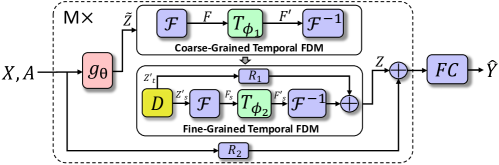
Figure S1: An illustration of Temporal Graph GegenConv (TGC), where $g_{\theta}(\cdot)$, $\mathcal{T}_{\phi_{1}}(\cdot)$, and $\mathcal{T}_{\phi_{2}}(\cdot)$ are GSFs and two different TSFs. We use DFT and IDFT as $\mathcal{F}(\cdot)$ and $\mathcal{F}^{-1}(\cdot)$ in our implementation.

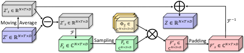
Figure S2: Tensor flow in fine-grained temporal frequency-domain models.

D.2 Time Series Decomposition

Given a time series $\mathbf{x}\in\mathbb{R}^{T}$, we extract its trend information by conducting moving average with a window size $w$ on the input signal, i.e., $\tilde{\mathbf{x}}(t)=\big{(}\mathbf{x}(t-w+1)+\cdots+\mathbf{x}(t)\big{)}/w$, where we simply pad the first $w-1$ data points with zeros in $\tilde{\mathbf{x}}$. After this, we obtain detailed time series information (e.g., seasonality) by subtracting the trend from the input signal.

D.3 Component Padding

We employ discrete Fourier transformations as space projections by default in TGC and TGC^†. We pad the filtered signal tensors in both the coarse-grained and fine-grained temporal FDMs with $0+0j$, thereby reshaping them from $\mathbb{C}^{N\times S\times D}$ to $\mathbb{C}^{N\times T\times D}$. An illustration of this can be seen in Figure S2.

D.4 Nonlinearities

Nonlinearities can be either applied in graph and/or temporal frequency-domain models. We apply both in TGC^†. In the first case, we add the ReLU activation $\sigma(\cdot)$ as follows.

$$g(\mathbf{\Lambda})\star\mathbf{X}_{t}:=g_{\theta}(\hat{\mathbf{L}})\sigma{(\mathbf{X}_{t})}.$$ (S21)

In the second case, we have Equation 3 and Equation 4 modified as follows.

$$\mathbf{F} =\mathcal{F}(\tilde{\mathbf{Z}}), \hskip 5.0pt\mathbf{F}^{\prime} =\textsc{Pad}(\sigma(\mathbf{F}\mathbf{S}^{\top}_{1}\mathbf{\Phi}_{1})), \hskip 5.0pt\mathbf{Z}^{\prime} =\mathcal{F}^{-1}(\mathbf{F}^{\prime}).$$ (S22)

$$\mathbf{Z}^{\prime}_{t},\mathbf{Z}^{\prime}_{s} =\textsc{Decomp}(\mathbf{Z}^{\prime}), \mathbf{F}_{s} =\mathcal{F}(\mathbf{Z}^{\prime}_{s}), \mathbf{F}^{\prime}_{s} =\textsc{Pad}(\sigma(\mathbf{F}_{s}\mathbf{S}^{\top}_{2}\mathbf{\Phi}_{2})), \mathbf{Z} =\mathbf{Z}^{\prime}_{t}+\mathcal{F}^{-1}(\mathbf{F}^{\prime}_{s}).$$ (S23)

D.5 Spectral Attention

Attention in spectral domains [14] can be easily incorporated in temporal frequency-domain models. In TGC^†, we implement the spectral filters in fine-grained temporal FDMs with spectral attention instead of Equation S23.

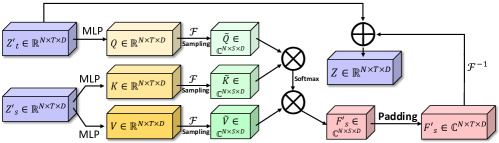
Figure S3: Tensor flow in fine-grained temporal frequency-domain models using spectral attention.

Specifically, we first decompose the input signal via $\mathbf{Z}^{\prime}_{t},\mathbf{Z}^{\prime}_{s}=\textsc{Decomp}(\mathbf{Z}^{\prime})$. After this, we generate the queries $\mathbf{Q}=\sigma(\mathbf{\Phi}_{2,1}\mathbf{Z}^{\prime}_{t})\in\mathbb{R}^{N\times T\times D}$, keys $\mathbf{K}=\sigma(\mathbf{\Phi}_{2,2}\mathbf{Z}^{\prime}_{s})\in\mathbb{R}^{N\times T\times D}$, and values $\mathbf{V}=\sigma(\mathbf{\Phi}_{2,3}\mathbf{Z}^{\prime}_{s})\in\mathbb{R}^{N\times T\times D}$. $\sigma(\cdot)$ denotes the ReLU activation. Then, we project all three matrices into the frequency domain via the discrete Fourier transformation, i.e., $\tilde{\mathbf{Q}}=\mathcal{F}(\mathbf{Q})\mathbf{S}^{\top}_{2,1}\in\mathbb{C}^{N\times S\times D}$, $\tilde{\mathbf{K}}=\mathcal{F}(\mathbf{K})\mathbf{S}^{\top}_{2,2}\in\mathbb{C}^{N\times S\times D}$, and $\tilde{\mathbf{V}}=\mathcal{F}(\mathbf{V})\mathbf{S}^{\top}_{2,3}\in\mathbb{C}^{N\times S\times D}$. Finally, we select informative components with

$$\mathbf{F}^{\prime}_{s}=\textsc{Softmax}(\frac{\tilde{\mathbf{Q}}\tilde{\mathbf{K}}^{\top}}{\sqrt{n_{q}d_{q}}})\tilde{\mathbf{V}}.$$ (S24)

Now we obtain the learned embeddings via $\mathbf{Z}=\mathbf{Z}^{\prime}_{t}+\mathcal{F}^{-1}\big{(}\textsc{Pad}(\mathbf{F}^{\prime}_{s})\big{)}$. We illustrate the tensor flow of this process in Figure S3.

Appendix E Connection to Other Polynomial Bases

We compare our instantiation with common practices in approximating graph convolutions: Monomial, Chebyshev, Bernstein, and Jacobi bases. We visualize these polynomial bases with limited degrees in Figure S4.

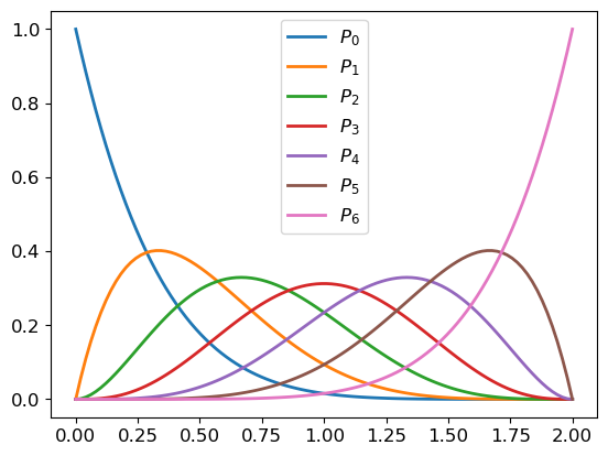
(a) Bernstein basis

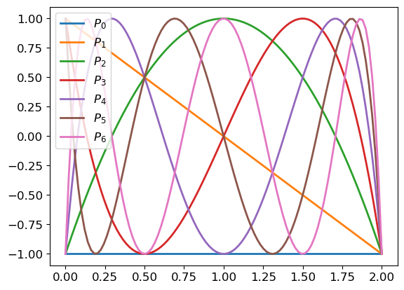
(b) Chebyshev basis

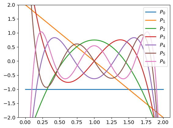
(c) Gegenbauer basis

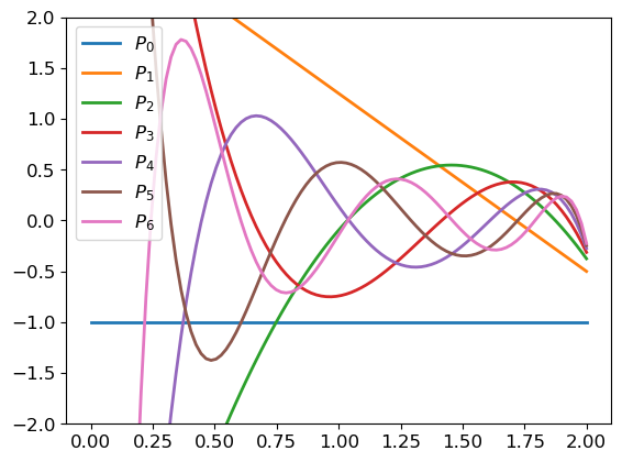
(d) Jacobi basis

Figure S4: Different polynomial bases in approximating graph convolutions.

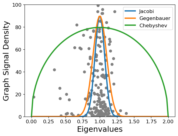
(a) PeMS03 Dataset

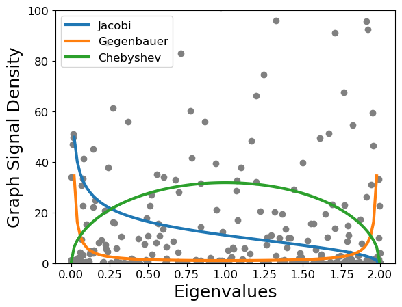
(b) PeMS04 Dataset

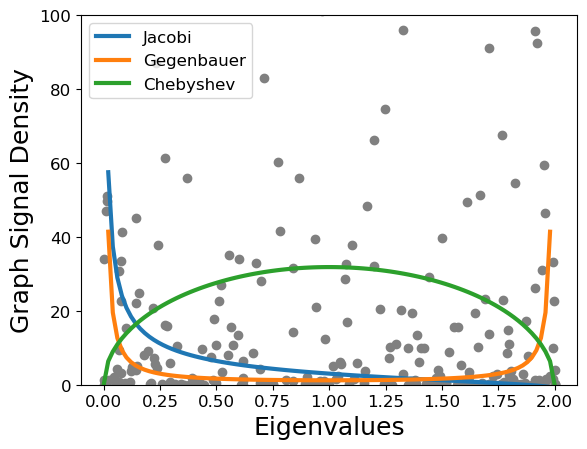
(c) PeMS07 Dataset

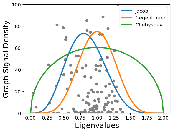
(d) PeMS08 Dataset

Figure S5: Signal density of predefined graphs on different datasets at a randomly selected time step versus the best-fitted weight functions of three different orthogonal polynomials.

For the Monomial basis $(1-\lambda)^{k}$, it is non-orthogonal for arbitrary choices of weight functions [13]. Although the Bernstein basis $\binom{K}{k}(1-\frac{\lambda}{2})^{K-k}(\frac{\lambda}{2})^{k}$ is also non-orthogonal, existing studies show that a small conditional number of the Hessian matrix $\kappa{(\mathbf{\mathbf{H}})}$ may still be achieved to enable fast convergence, where $\kappa{(\mathbf{\mathbf{H}})}$ can also be lower than using Monomial basis marco2010polynomial. While the Bernstein basis is better than the Monomial basis in approximating graph convolutions, our instantiation with the Gegenbauer basis guarantees the minimum $\kappa{(\mathbf{\mathbf{H}})}$ to be achieved in most cases; thus, it is more desired. We provide examples in Figure S5 showing that the weight functions of Gegenbauer polynomials fit graph signal densities well in most cases. Our main results also confirm this in Table 4.

For orthogonal polynomials, the second-kind Chebyshev basis is a particular case of the Gegenbauer basis with $\alpha=1$ and only orthogonal w.r.t. a particular weight $\sqrt{1-\lambda^{2}}$. Though the Gegenbauer basis forms a particular case of the Jacobi basis with both of its parameters set to $\alpha-\frac{1}{2}$, we show that the orthogonality of the Gegenbauer basis is well-posed on common real-world graphs w.r.t. its weight function $(1-\lambda^{2})^{\alpha-\frac{1}{2}}$ as shown in Figure S5. Thus, in this work, we use the Gegenbauer basis as a simpler solution for our purpose with only minor performance degradation (Table 4).

Appendix F Datasets

Table S1: Statistics of eight different real-world time series datasets used in our work.

Statistic	PeMS03	PeMS04	PeMS07	PeMS08	Electricity	Solar	Weather	ECG
# of time series	358	307	228	170	321	137	21	140
# of data points	26,209	16,992	12,672	17,856	26,304	52,560	52,696	5,000
Sampling rate	5 min	5 min	5 min	5 min	1 hour	10 min	10 min	-
Predefined graph	Yes	Yes	Yes	Yes	No	No	No	No

• PeMS03, 04, 07, and 08: These datasets are collected by the Caltrans Performance Measurement System (PeMS) from traffic sensors installed in highway systems spanned across metropolitan areas in California. The sampling rate of these datasets is 5 minutes, where PeMS03, 07, and 08 record traffic flow, and PeMS04 is about traffic speed.

• Electricity: This dataset consists of electricity consumption records of 321 customers with 1-hour sampling rate.

• Solar-Energy³: This dataset consists of photovoltaic production records of 137 sites in Alabama State in 2006. The sampling rate in this dataset is 10 minutes.

• Weather: This dataset consists of the one-year records of 21 meteorological stations installed in Germany. The sampling rate in this dataset is 10 minutes.

• ECG: This dataset consists of the 5000 records of 140 electrocardiograms in the URC time series archive.

Appendix G Experimental Setting

All experiments are conducted on a Linux server with $4\times$ GeForce RTX 2080 Ti 11GB, $1\times$ Intel Core i9-9900X, and 128GB system memory.

G.1 Short-Term Forecasting

Here, we detail the experimental setting of short-term time series forecasting. Our main results are in Table 1 and Table S4. The dataset statistics are in Table S1. We briefly introduce all baselines as follows.

• FC-LSTM sutskever2014sequence forecasts a time series with fully-connected long short-term memory units.

• TCN bai2018empirical forecasts time series data with stacked dilated convolutions.

• LSTNet [19] uses convolutions to mine local time series dependencies and recurrent neural networks to model temporal clues.

• DeepState [20] takes advantage of state space models, where time-related parameters are calculated via recurrent neural networks by digesting the input series.

• DeepGLO [21] leverages TCN regularized matrix factorization to capture global features, along with another set of temporal networks to capture local patterns of each time series.

• SFM zhang2017stock enhances long short-term memory units by breaking down cell states of a time series into a set of frequency components.

• DCRNN [22] integrates graph diffusion into recurrent neural networks to capture spatial and temporal relations in multivariate time series data.

• STGCN [2] combines ChebyConv [4] and temporal convolutions together into a decoupled neural architecture to capture spatial and temporal multivariate time series relations simultaneously. Note that STGCN$(1^{st})$ adopts the first-order approximation of ChebyConv.

• Graph WaveNet [3] integrates TCN and graph diffusion [5], along with a graph structure refinement mechanism, to learn spatial and temporal multivariate time series relations.

• ASTGCN [23] improves existing works with separate spatial and temporal attention. Note that MSTGCN is a variant of ASTGCN with all attention mechanisms disabled.

• STG2Seq [24] proposes to capture both spatial and temporal correlations simutaneously with hierarchical graph convolutions adapted from GCN kipf2016semi.

• LSGCN [25] introduces the spatial gated block with a novel attention-enhanced graph convolution network to better capture spatial dependencies in STGNNs.

• STSGCN [26] proposes a space-time-separable graph convolution network to models entire graph dynamics with only graph convolution networks adapted from GCN kipf2016semi.

• STFGNN [27] incorporates various time series correlation mining strategies to learn spatial-temporal fusion graphs that facilitate the learning of latent spatial and temporal dependencies.

• STGODE [28] introduces spatial-temporal graph ordinary differential equation networks to better capture both short- and long-range spatial correlations compared with other STGNNs.

• StemGNN [7] marries ChebyConv and temporal frequency-domain models to model time series spatial and temporal dependencies in spectral domains.

General experimental setting.

We adopt the Mean Absolute Forecasting Errors (MAE) and Root Mean Squared Forecasting Errors (RMSE) as evaluation metrics. On three traffic datasets (i.e., PeMS03, 04, and 08), we use the data split of 60%-20%-20%. On the rest of the time series datasets, i.e., PeMS07, Electricity, Solar-Energy, and ECG, we follow [7] and use the split ratio of 70%-20%-10%. For data preprocessing, we use min-max normalization and Z-Score normalization on ECG and the rest of the datasets, respectively. On four traffic datasets (i.e., PeMS03, 04, 07, and 08), we use the past 1-hour observations to predict the next 15-minute traffic volume or speed. We also use this setting in ablation studies and model efficiency comparisons. On the Electricity dataset, we forecast the next 1-hour consumption with the past 24-hour readings. On the Solar-Energy dataset, we use the past 4-hour data to predict the productions in the next half hour. On the ECG dataset, we set the window size and forecasting horizon to 12 and 3. For the baseline configurations, we follow [7]. For the primary hyperparameter settings of TGC on different datasets, see Table S2.

Experimental setting in Table 1 (right).

We adopt the same evaluation metrics and follow the experimental setting in [18]. For the four traffic datasets, we use a data split of 60%-20%-20%. In terms of data preprocessing, min-max normalization is employed. Here, we use the past 1-hour observations to predict the next 1-hour traffic volume or speed.

Table S2: The hyperparameter setting of TGC for short-term time series forecasting.

Hyperparameters	PeMS03	PeMS04	PeMS07	PeMS08	Electricity	Solar	ECG
Gegenbauer parameter $\alpha$	3.08	0.47	1	1	1.2	1.2	1.2
# polynomial degree $K$	4	4	4	4	4	4	4
# selected component $S$	5	4	5	5	5	5	5
# building block $M$	2	2	2	2	2	2	2
Training batch size B	32	64	50	50	50	50	50
Model learning rate $\eta$	0.0003	0.001	0.001	0.001	0.001	0.001	0.001

G.2 Long-Term Forecasting

In this subsection, we detail the experimental setting of long-term time series forecasting. Our results are in Table 2. The dataset statistics are in Table S1. For all baselines, we detail them as follows.

• FiLM [29] first applies Legendre polynomial to approximate time series and then denoises approximations with a frequency-domain model based on Fourier projections.

• FEDformer [14] proposes a frequency-enhanced Transformer framework for effective long-term time series forecasting.

• Autoformer [30] designs a decomposition Transformer with the auto-correlation mechanism for long-term time series forecasting.

• Informer [31] is an efficient Transformer with ProbSparse self-attention for long-term time series forecasting.

• LogTrans [32] uses LogSparse attention to implement an efficient Transformer for time series forecasting.

• Reformer [33] marries local-sensitive hashing with Transformer to significantly reduce the model complexity.

Similar to short-term forecasting, we adopt the MAE and RMSE as evaluation matrices. For dataset split and baseline settings, we follow [29]. Specifically, we use the split of 70%-10%-20% for all three datasets. On the Electricity dataset, we use the past 4 days’ observations to predict the consumption of the next 4, 8, and 14 days. On the Solar-Energy and Weather datasets, we predict the next 16, 32, and 56 hours’ readings by using the past 16-hour data. It is worth noting that we use Jacobi polynomial basis for long-term forecasting by default, which has two tunable parameters $\alpha$ and $\beta$ (See Appendix E). The hyperparameter setting of our method for long-term forecasting is in Table S3.

Table S3: The hyperparameter setting of TGC for long-term time series forecasting.

Hyperparameters	$\alpha$	$\beta$	$K$	$S$	$M$	$B$	$\eta$
Electricity	1	1	4	14	5	50	0.001
Solar-Energy	1	1	4	50	5	50	0.001
Weather	0.81	0.90	4	26	3	64	0.0003

G.3 Evaluation of Modeling Differently Signed Time Series Relations

We now describe the generation of the synthetic dataset used in our experiments in 6(a). To assess our method’s ability to model differently signed time series relations, we create two groups of time series, each with a length of 2000. For the first group, we generate a sinusoidal signal and develop 100 distinct instances with varying amplitudes and injected random noise. Similarly, we generate another group of data based on cosinusoidal oscillation. Consequently, we know that: (1) Time series within each group are positively correlated; (2) Time series across different groups are negatively correlated. We denote these two groups as types A and B in our experiments. Referring to our discussion and the results in 6(a), we make two clear observations: (1) Both our method (i.e., TGC) and MP-STGNNs can learn positive relations between time series (i.e., same colored shapes should be close to each other); (2) However, only our method can model differently signed (e.g., purely negatively correlated) time series (i.e., differently colored shapes should be far away from each other).

Appendix H Additional Results

H.1 Additional Forecasting Results

Table S4: Additional short-term forecasting results on three general time series benchmarks, where we follow [7] for the experimental setting and baseline results. We use the bold and underline fonts to indicate the best and second-best results.

Method	MAE	RMSE	MAE	RMSE	MAE	RMSE
	Electricity		Solar		ECG
FC-LSTM	0.62	0.20	0.13	0.19	0.32	0.54
TCN	0.07	0.51	0.06	0.06	0.10	0.30
LSTNet	0.06	0.07	0.07	0.19	0.08	0.12
DeepState	0.06	0.67	0.06	0.25	0.09	0.76
DeepGLO	0.08	0.14	0.09	0.14	0.09	0.15
SFM	0.08	0.13	0.05	0.09	0.17	0.58
Graph WaveNet	0.07	0.53	0.09	0.14	0.09	0.15
StemGNN	0.04	0.06	0.03	0.07	0.05	0.07
TGC (Ours)	0.05	0.07	0.02	0.04	0.04	0.06

We provide our supplementary short-term forecasting results in Table S4, from which the following observations can be made: (1) TGC, in most cases, outperforms all baseline methods by substantial margins, with an average improvement of 35% compared to the best deep time series baselines; (2) It generally outperforms StemGNN, although the performance gaps are not very significant under this experimental setting.

H.2 Parameter Studies

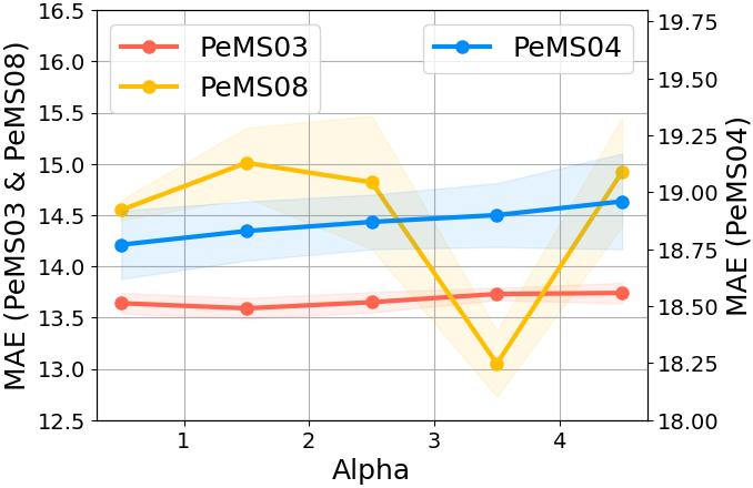
(a) Study on the Gegenbauer parameter $\alpha$.

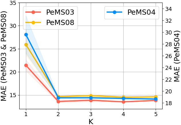
(b) Study on the polynomial degree $K$

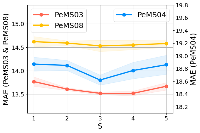
(c) Study on the number of selected modes $S$.

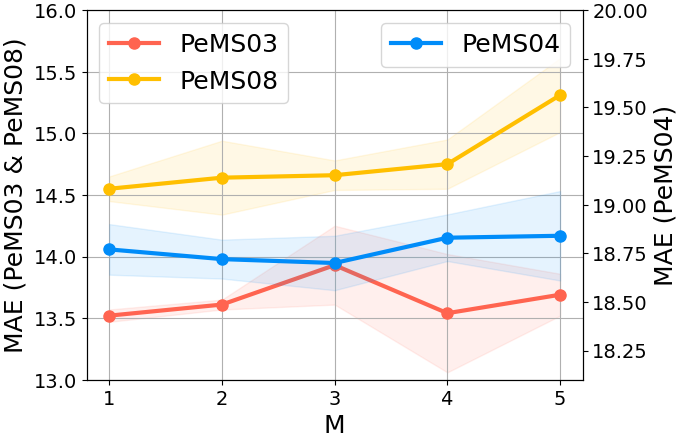
(d) Study on the number of building blocks $M$.

Figure S6: Study on important parameters in TGC.

In Figure S6, we study four important hyperparameters in TGC. Our experimental results lead to the following observations: (1) Adjusting the $\alpha$ in Gegenbauer polynomials impacts model performance variably across datasets. For instance, a smaller $\alpha$ is generally favored in three PeMS datasets, as depicted in 6(a); (2) The polynomial degree should not be too small to avoid information loss, as demonstrated by the poor performance when $K=1$ in 6(b). In practice, we set $K$ between 3 and 5, as higher degrees do not bring additional performance gains; (3) Similarly, setting $S$ too small or too large is not desirable, as shown in 6(c). This is to prevent information loss and mitigate the impact of noise; (4) Stacking more building blocks seems to result in better performance, as illustrated in 6(d). However, this comes at the cost of model efficiency.

H.3 Additional Evaluation of Modeling Time Series Dependencies

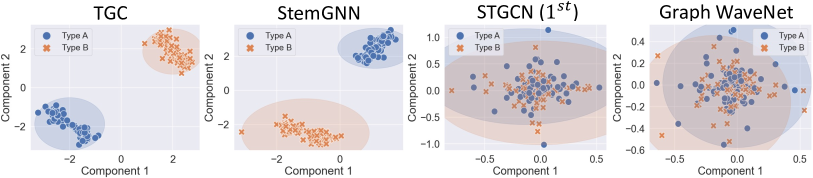
Figure S7: Additional comparison between learned embeddings w.r.t. different time series correlations on a synthetic dataset presented in 6(a). Types A and B denote series groups exhibiting opposing trends. Differently colored shading indicates distinct clusters.

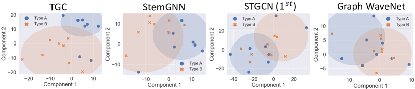
Figure S8: Additional comparison between learned embeddings w.r.t. different time series correlations on a subset of traffic recordings in PeMS07 dataset as presented in 6(b). Types A and B denote series groups exhibiting opposing trends. Differently colored shading indicates distinct clusters.

Additional evaluation can be found in Figure S7 and Figure S8, where we compare the learned time series embeddings from two SPTGNNs (i.e., Ours and StemGNN [7]) and MP-STGNNs (i.e., STGCN$(1^{st})$ [2] and Graph WaveNet [3]). It is evident that SPTGNNs excel in learning different signed spatial relations between time series, yielding significantly distinct representations with much higher clustering purities in both cases, further substantiating our claims in the main text.

H.4 Additional Main Result Statistics

Table S5 presents both the average performances and 95% confidence intervals for our results reported in Table 1 and Table 2 with five individual runs on seven real-world time series datasets, covering both short-term and long-term forecasting tasks.

Table S5: Short-term and long-term forecasting results showing our average performances $\pm 95\%$ confidence intervals, respectively.

Method		TGC		TGC†
		MAE	RMSE	MAE	RMSE
PeMS03	3	13.52 $\pm$ 0.226	21.74 $\pm$ 0.687	-	-
	12	-	-	16.22 $\pm$ 0.475	27.07 $\pm$ 0.623
PeMS04	3	18.77 $\pm$ 0.142	29.92 $\pm$ 0.150	-	-
	12	-	-	20.00 $\pm$ 0.300	32.10 $\pm$ 0.452
PeMS07	3	1.92 $\pm$ 0.029	3.35 $\pm$ 0.093	-	-
	12	-	-	2.81 $\pm$ 0.035	5.58 $\pm$ 0.066
PeMS08	3	14.55 $\pm$ 0.245	22.73 $\pm$ 0.274	-	-
	12	-	-	16.54 $\pm$ 0.981	26.10 $\pm$ 0.825

Method		TGC†
		MAE	RMSE
Electricity	96	0.293 $\pm$ 0.004	0.425 $\pm$ 0.006
	192	0.303 $\pm$ 0.006	0.440 $\pm$ 0.007
	336	0.313 $\pm$ 0.007	0.470 $\pm$ 0.005
Weather	96	0.235 $\pm$ 0.014	0.408 $\pm$ 0.029
	192	0.286 $\pm$ 0.021	0.468 $\pm$ 0.041
	336	0.317 $\pm$ 0.019	0.515 $\pm$ 0.036
Solar	96	0.242 $\pm$ 0.005	0.443 $\pm$ 0.009
	192	0.263 $\pm$ 0.004	0.470 $\pm$ 0.010
	336	0.271 $\pm$ 0.004	0.478 $\pm$ 0.009

Appendix I Visualization

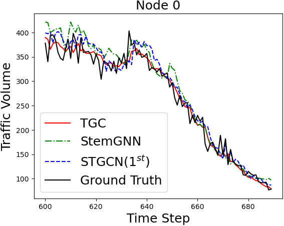
(a) Predictions on node 0 (1st selected period on PeMS08)

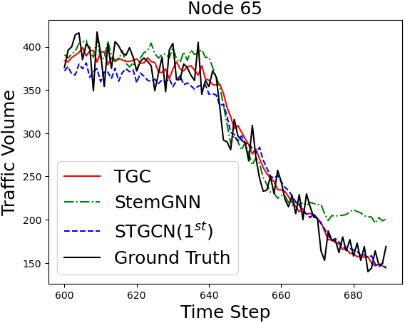
(b) Predictions on node 65 (1st selected period on PeMS08)

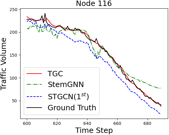
(c) Predictions on node 116 (1st selected period on PeMS08)

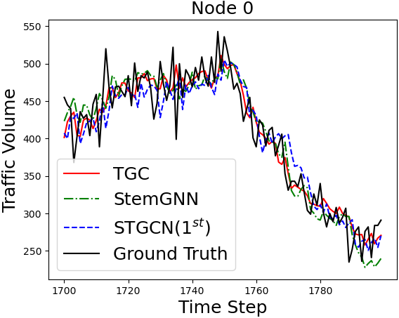
(d) Predictions on node 0 (2nd selected period on PeMS08)

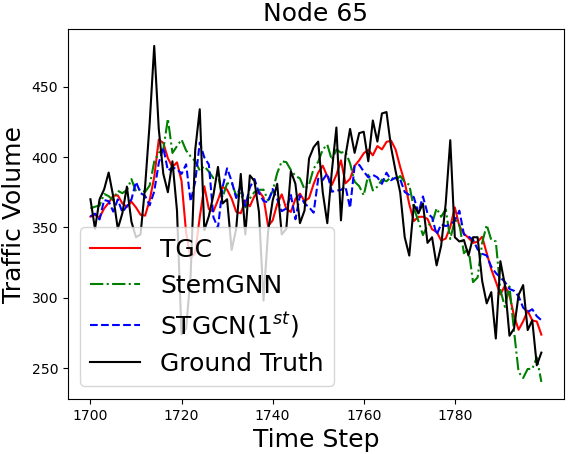
(e) Predictions on node 65 (2nd selected period on PeMS08)

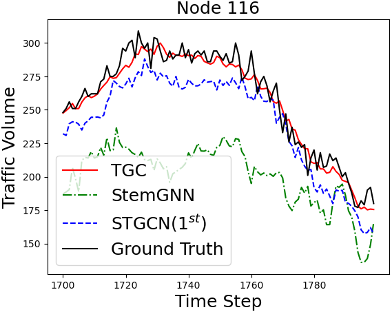
(f) Predictions on node 116 (2nd selected period on PeMS08)

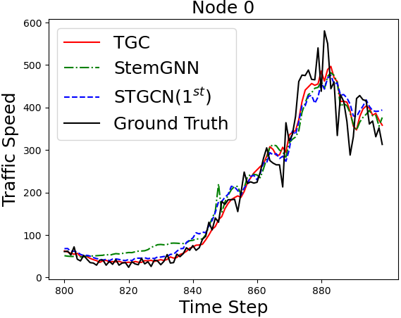
(g) Predictions on node 0 (1st selected period on PeMS04)

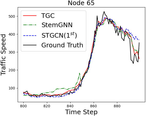
(h) Predictions on node 65 (1st selected period on PeMS04)

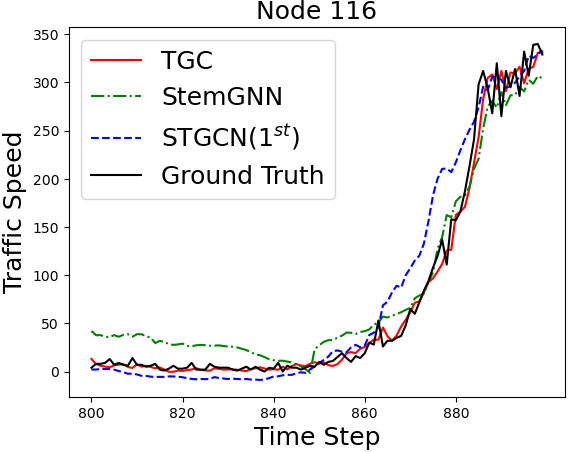
(i) Predictions on node 116 (1st selected period on PeMS04)

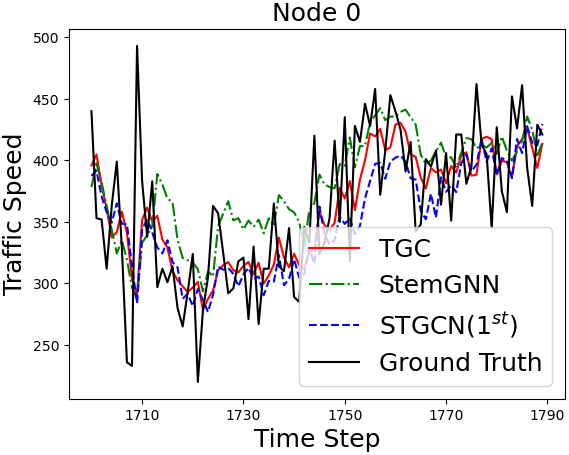
(j) Predictions on node 0 (2nd selected period on PeMS04)

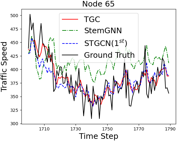
(k) Predictions on node 65 (2nd selected period on PeMS04)

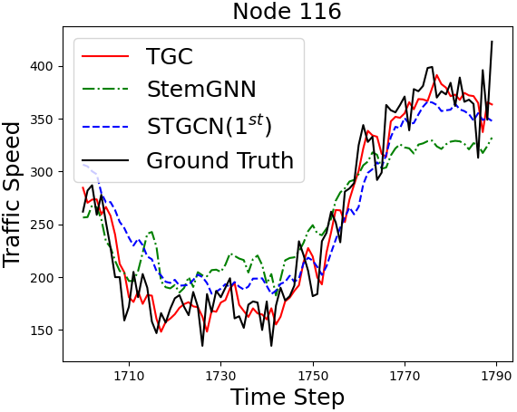
(l) Predictions on node 116 (2nd selected period on PeMS04)

Figure S9: Forecasting visualizations of TGC, StemGNN, and STGCN$(1^{st})$ on PeMS08 and PeMS04 datasets are shown in the first and last six subplots, which we refer to as groups A and B. In each group, the first and last three subplots present visualizations for three randomly selected sensors at two different periods on the test sets.

unsrtnat reference

References

- Hamilton [2020] William L Hamilton. Graph representation learning. Synthesis Lectures on Artificial Intelligence and Machine Learning, 14(3):1–159, 2020.
- Yu et al. [2018] Bing Yu, Haoteng Yin, and Zhanxing Zhu. Spatio-temporal graph convolutional networks: A deep learning framework for traffic forecasting. In International Joint Conferences on Artificial Intelligence, pages 3634–3640, 2018.
- Wu et al. [2019] Zonghan Wu, Shirui Pan, Guodong Long, Jing Jiang, and Chengqi Zhang. Graph wavenet for deep spatial-temporal graph modeling. In International Joint Conference on Artificial Intelligence, pages 1907–1913, 2019.
- Defferrard et al. [2016] Michaël Defferrard, Xavier Bresson, and Pierre Vandergheynst. Convolutional neural networks on graphs with fast localized spectral filtering. In Advances in Neural Information Processing Systems, pages 3837–3845, 2016.
- Klicpera et al. [2019] Johannes Klicpera, Stefan Weißenberger, and Stephan Günnemann. Diffusion improves graph learning. In Advances in Neural Information Processing Systems, pages 13366–13378, 2019.
- Li et al. [2021] Shouheng Li, Dongwoo Kim, and Qing Wang. Beyond low-pass filters: Adaptive feature propagation on graphs. In Joint European Conference on Machine Learning and Knowledge Discovery in Databases, pages 450–465. Springer, 2021.
- Cao et al. [2020] Defu Cao, Yujing Wang, Juanyong Duan, Ce Zhang, Xia Zhu, Congrui Huang, Yunhai Tong, Bixiong Xu, Jing Bai, Jie Tong, et al. Spectral temporal graph neural network for multivariate time-series forecasting. In Advances in neural information processing systems, volume 33, pages 17766–17778, 2020.
- He et al. [2021] Mingguo He, Zhewei Wei, Hongteng Xu, et al. Bernnet: Learning arbitrary graph spectral filters via bernstein approximation. In Advances in Neural Information Processing Systems, volume 34, pages 14239–14251, 2021.
- Derr et al. [2018] Tyler Derr, Yao Ma, and Jiliang Tang. Signed graph convolutional networks. In IEEE International Conference on Data Mining, pages 929–934. IEEE, 2018.
- Jin et al. [2022a] Ming Jin, Yu Zheng, Yuan-Fang Li, Siheng Chen, Bin Yang, and Shirui Pan. Multivariate time series forecasting with dynamic graph neural odes. IEEE Transactions on Knowledge and Data Engineering, 2022a.
- Luo et al. [2023] Linhao Luo, Gholamreza Haffari, and Shirui Pan. Graph sequential neural ode process for link prediction on dynamic and sparse graphs. In Proceedings of the Sixteenth ACM International Conference on Web Search and Data Mining, pages 778–786, 2023.
- Jin et al. [2022b] Ming Jin, Yuan-Fang Li, and Shirui Pan. Neural temporal walks: Motif-aware representation learning on continuous-time dynamic graphs. In Advances in Neural Information Processing Systems, 2022b.
- Wang and Zhang [2022] Xiyuan Wang and Muhan Zhang. How powerful are spectral graph neural networks. In International Conference on Machine Learning, 2022.
- Zhou et al. [2022a] Tian Zhou, Ziqing Ma, Qingsong Wen, Xue Wang, Liang Sun, and Rong Jin. Fedformer: Frequency enhanced decomposed transformer for long-term series forecasting. In International Conference on Machine Learning, volume 162, pages 27268–27286. PMLR, 2022a.
- Souza et al. [2022] Amauri H Souza, Diego Mesquita, Samuel Kaski, and Vikas K Garg. Provably expressive temporal graph networks. In Advances in Neural Information Processing Systems, 2022.
- Wallace and Dickinson [1972] John M Wallace and Robert E Dickinson. Empirical orthogonal representation of time series in the frequency domain. part i: Theoretical considerations. Journal of Applied Meteorology and Climatology, 11(6):887–892, 1972.
- Poli et al. [2022] Michael Poli, Stefano Massaroli, Federico Berto, Jinkyoo Park, Tri Dao, Christopher Re, and Stefano Ermon. Transform once: Efficient operator learning in frequency domain. In Advances in Neural Information Processing Systems, 2022.
- Choi et al. [2022] Jeongwhan Choi, Hwangyong Choi, Jeehyun Hwang, and Noseong Park. Graph neural controlled differential equations for traffic forecasting. In Proceedings of the AAAI Conference on Artificial Intelligence, pages 6367–6374, 2022.
- Lai et al. [2018] Guokun Lai, Wei-Cheng Chang, Yiming Yang, and Hanxiao Liu. Modeling long- and short-term temporal patterns with deep neural networks. In Proceedings of 41st International ACM SIGIR Conference on Information Retrieval, pages 95–104. ACM, 2018.
- Rangapuram et al. [2018] Syama Sundar Rangapuram, Matthias W. Seeger, Jan Gasthaus, Lorenzo Stella, Yuyang Wang, and Tim Januschowski. Deep state space models for time series forecasting. In Advances in Neural Information Processing Systems, pages 7796–7805, 2018.
- Sen et al. [2019] Rajat Sen, Hsiang-Fu Yu, and Inderjit S Dhillon. Think globally, act locally: A deep neural network approach to high-dimensional time series forecasting. In Advances in neural information processing systems, volume 32, 2019.
- Li et al. [2018] Yaguang Li, Rose Yu, Cyrus Shahabi, and Yan Liu. Diffusion convolutional recurrent neural network: Data-driven traffic forecasting. In International Conference on Learning Representations, 2018.
- Guo et al. [2019] Shengnan Guo, Youfang Lin, Ning Feng, Chao Song, and Huaiyu Wan. Attention based spatial-temporal graph convolutional networks for traffic flow forecasting. In Proceedings of the AAAI Conference on Artificial Intelligence, volume 33, pages 922–929, 2019.
- Bai et al. [2019] Lei Bai, Lina Yao, Salil S Kanhere, Xianzhi Wang, and Quan Z Sheng. Stg2seq: spatial-temporal graph to sequence model for multi-step passenger demand forecasting. In International Joint Conferences on Artificial Intelligence, pages 1981–1987, 2019.
- Huang et al. [2020] Rongzhou Huang, Chuyin Huang, Yubao Liu, Genan Dai, and Weiyang Kong. Lsgcn: Long short-term traffic prediction with graph convolutional networks. In International Joint Conferences on Artificial Intelligence, volume 7, pages 2355–2361, 2020.
- Sofianos et al. [2021] Theodoros Sofianos, Alessio Sampieri, Luca Franco, and Fabio Galasso. Space-time-separable graph convolutional network for pose forecasting. In Proceedings of the IEEE/CVF International Conference on Computer Vision, pages 11209–11218, 2021.
- Li and Zhu [2021] Mengzhang Li and Zhanxing Zhu. Spatial-temporal fusion graph neural networks for traffic flow forecasting. In Proceedings of the AAAI conference on artificial intelligence, pages 4189–4196, 2021.
- Fang et al. [2021] Zheng Fang, Qingqing Long, Guojie Song, and Kunqing Xie. Spatial-temporal graph ode networks for traffic flow forecasting. In Proceedings of the 27th ACM SIGKDD conference on knowledge discovery & data mining, pages 364–373, 2021.
- Zhou et al. [2022b] Tian Zhou, Ziqing Ma, xue wang, Qingsong Wen, Liang Sun, Tao Yao, Wotao Yin, and Rong Jin. Film: Frequency improved legendre memory model for long-term time series forecasting. In Advances in Neural Information Processing Systems, 2022b.
- Wu et al. [2021] Haixu Wu, Jiehui Xu, Jianmin Wang, and Mingsheng Long. Autoformer: Decomposition transformers with auto-correlation for long-term series forecasting. In Advances in Neural Information Processing Systems, volume 34, pages 22419–22430, 2021.
- Zhou et al. [2021] Haoyi Zhou, Shanghang Zhang, Jieqi Peng, Shuai Zhang, Jianxin Li, Hui Xiong, and Wancai Zhang. Informer: Beyond efficient transformer for long sequence time-series forecasting. In Proceedings of the AAAI Conference on Artificial Intelligence, pages 11106–11115, 2021.
- Li et al. [2019] Shiyang Li, Xiaoyong Jin, Yao Xuan, Xiyou Zhou, Wenhu Chen, Yu-Xiang Wang, and Xifeng Yan. Enhancing the locality and breaking the memory bottleneck of transformer on time series forecasting. In Advances in neural information processing systems, volume 32, 2019.
- Kitaev et al. [2020] Nikita Kitaev, Lukasz Kaiser, and Anselm Levskaya. Reformer: The efficient transformer. In International Conference on Learning Representations, 2020.