Self-steepening-induced stabilization of nonlinear edge waves
at photonic valley-Hall interfaces
Abstract
Localized nonlinear modes at valley-Hall interfaces in staggered photonic graphene can be described in the long-wavelength limit by a nonlinear Dirac-like model including spatial dispersion terms. It leads to a modified nonlinear Schrödinger equation for the wave field amplitude that remarkably incorporates a nonlinear velocity term. We show that this nonlinear velocity correction results in a counter-intuitive stabilization effect for relatively high-amplitude plane-wave-like edge states, which we confirm by calculation of complex-valued small-amplitude perturbation spectra and direct numerical simulation of propagation dynamics in staggered honeycomb waveguide lattices with on-site Kerr nonlinearity. Our findings are relevant to a variety of nonlinear photonic systems described by Dirac-like Hamiltonians.
I I. Introduction
Topological edge modes are the indicative hallmark of the topologically nontrivial systems that can be characterised by the quantised invariants of the bulk eigenspectrum. Driven by inspiration from the solid-state physics, they were observed in many engineered photonic platforms including waveguide arrays and photonic crystals Ozawa2019 . Their dispersion can often be captured by effective Dirac-like models. Their transformations induced by nonlinear effects in optical systems constitute an important subject of research in pursuit of potential applications in high-speed photonic circuits and communication networks Smirnova2020APR .
Modulational instability is a phenomenon that appears in many nonlinear systems in nature as a result of the interplay between the nonlinearity and dispersion. In the course of this process development even minor disturbances to the stationary state in a nonlinear system experience exponential growth over time. For the boundary problem, it may in turn apply to the edge waves that propagate along the topological domain walls,; even when protected against backscattering these waves can become unstable under long-wavelength perturbations and break down into localized structures. Modulational instability can be used to probe bulk topological invariants leykam2021probing ; maluckov2022nonlinear ; mancic2023band and plays an important role in edge soliton formation lumer2016instability ; kartashov2016modulational ; zhang2019interface ; smirnova2021gradient .
Recent observations of optical solitons in Floquet topological lattices Maczewsky2020 ; Mukherjee2020 ; Mukherjee2021 and other related phenomena, such as nonlinear Thouless pumping Jrgensen2021 ; Jrgensen2023 , implemented in periodically modulated waveguide arrays reflect ongoing experimental interest in nonlinear effects in topological bands. It is argued that valley-Hall photonic lattices, being simple in design with no need for helical modulation, can be used to combine slow-light enhancement of nonlinear effects with topological protection against back reflection and disorder Rechtsman2019 ; Sauer2020 ; Arregui2021 . Nevertheless, their performance versus conventional (non-topological) waveguides is still under debate and sensitive to the fabrication tolerance of the specific design implementation, as discussed in the recent experimental work Ref. rosiek2023observation demonstrating enhanced backscattering in valley-Hall photonic crystal slabs.
Most previous studies lumer2016instability ; kartashov2016modulational ; zhang2019interface noted that the nonlinear counterparts of the topological edge modes in the optical systems with the self-focusing nonlinearity are modulationally unstable, and referred to the nonlinear Schrödinger equation (NSE) for the qualitative explanation Ablowitz2013 ; Ablowitz2014 ; lumer2016instability ; kartashov2016modulational ; Ivanov2020 ; Ivanov2020b . Here, we unravel the overlooked stabilization of the relatively high-amplitude nonlinear edge waves originating from the linear counterparts in the Dirac-like systems. It is rooted in the nonlinear velocity term correction to the NSE derived in Ref. smirnova2021gradient , which appears at interfaces between media with topological band gaps of finite width. The nonlinear velocity generally manifests itself in pulse self-steepening observable in experiments anderson1983nonlinear ; panoiu2009self ; travers2011ultrafast ; husko2015giant . The instability inhibition at larger powers can loosely be interpreted as balanced compensation between slowly moving humps and faster moving drops.
This paper begins by examining the linear stability of the nonlinear edge waves localized near domain walls in the framework of the generic nonlinear Dirac equations, using purely analytical asymptotic analysis put forward in our earlier works smirnova2019topological ; smirnova2021gradient . We then proceed to the discrete lattice model based on the tight-binding description before finally presenting numerical modeling of a realistic optical implementation using optical waveguide arrays. These steps collectively constitute a comprehensive methodological set and self-consistently confirm the stabilization effect.
II II. Continuum Nonlinear Dirac model
Our starting point is the nonlinear Dirac model (NDM) that describes that describes the spatiotemporal evolution of a two-component wavefunction :
| (1a) | |||
| (1d) | |||
where the off-diagonal spatial derivative operator in the valley-Hall systems is defined as smirnova2019topological ; smirnova2021gradient , and is the evolution coordinate, corresponding to propagation distance in case of waveguide arrays. Note, taking into account the second-order derivatives responsible for the spatial dispersion is significant for the correct description of the system behavior in the nonlinear regime, in particular, modulational instability, which is absent in the NDM with .
A topological domain wall is formally introduced by inverting the sign of the effective mass in two half-spaces, . We take parameter without loss of generality. The work smirnova2019topological presents the analytical solution for the propagating nonlinear edge modes confined to the interface at and possessing the profiles and nonlinear dispersion . Here is the intensity of this edge mode components at the interface. Although this formula for was derived at , it is still applicable in the vicinity of for small .
In Ref. smirnova2021gradient , we investigated dynamics of edge wavepackets that vary slowly along the direction and derived the evolution equation for the slowly varying amplitude , where is a travelling coordinate, of edge pulses with accuracy order (the small parameters are ):
| (2) |
It enters the asymptotic expression for the spinor components,
| (3) |
Equation (2) differs from the usual nonlinear Schrödinger equation (NSE) due to the presence of a second higher-order nonlinear term (second term on the right hand of the equation), which accounts for phase modulation and self-steepening effects, and constitutes the nonlinear velocity; higher amplitude edge waves travel more slowly. As discussed in Ref. smirnova2021gradient , the nonlinear velocity term is a consequence of the asymmetric intensity-dependent localization of the edge states in the direction transverse to the interface.
Based on Eq. (2), the nonlinear edge wave’s complex amplitude at the domain wall is given by
| (4) |
being exactly the steady state of this equation. In order to analyze stability of this state we apply a standard linear stability analysis by representing the perturbed solution in the form
| (5) |
Here are small perturbations. The eigenfrequency is a complex number obtained by solving the linear eigenvalue problem for the perturbations in the first order of accuracy upon substituting Eq. (5) into Eq. (2). The resulting dependence of on the modulation wavenumber determines stability of the edge state, with being the growth rate. If , the nonlinear state is stable and only exhibits small amplitude oscillations in the presence of perturbations. However, if , the nonlinear state is unstable, resulting in significant profile variations during propagation.
In this way, the growth rate is deduced to be
| (6) |
where we denote the parameter of nonlinearity . At , i.e., in the absence of dispersion, the nonlinear edge wave is stable. The positive radicand indicates instability. The instability condition can be formulated as follows,
| (7) |
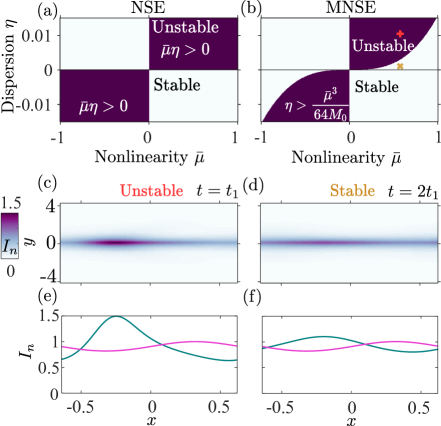
This analysis notably reveals the counter-intuitive finding that large-amplitude waves can be stable for the parameters obeying Eq. (7). Thus, once the nonlinear velocity is included into the modified nonlinear Schrödinger equation (MNSE), the instability area is reduced compared to the conventional NSE overlooking this contribution, as illustrated in Fig. 1(a,b). This means that the nonlinear velocity term has a stabilizing effect on the edge mode, making it less prone to decay. Examples of time evolution for modulationally unstable and stable edge waves modeled in the framework of NDM are shown in Figs. 1(c-f).
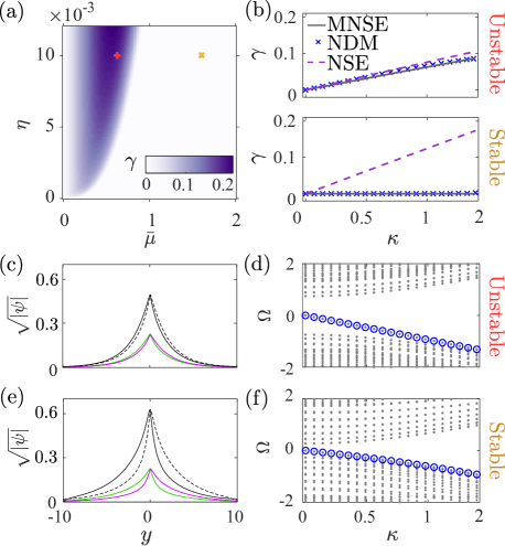
To verify our analytical predictions, we further calculate the perturbation spectra in Eq. (1) directly. To this end, we follow the procedure similar to the described above for Eq. (2) and analyse small perturbations to the numerically found nonlinear stationary solution at . The transverse profiles of the nonlinear mode components are visualized in Fig. 2(c,e) in black color. They exhibit noticeable asymmetry with the respect to the domain wall in the higher-intensity stable wave. We substitute the functions into Eq.(1) assuming the modulation of the form . The obtained spectrum of localized near domain wall linear perturbations is depicted in Fig. 2. We then fix the dispersion parameter and consider two different nonlinearity strengths corresponding to stable and unstable scenarios. As seen, the MNSE and Eq. (6) provides a more accurate approximation of the growth rate for unstable cases than NSE. Moreover, the stabilization effect is observable only in the framework of MNSE, while entirely absent in the conventional NSE. Note, however, we can correctly predict the growth rate until the real part of perturbation’s frequency, undergoing the nonlinearity-caused shift, crosses the bulk band. At that point, the approximate analytical approach breaks down, since the perturbations are no longer localized near the domain wall.
III III. Staggered graphene lattice model
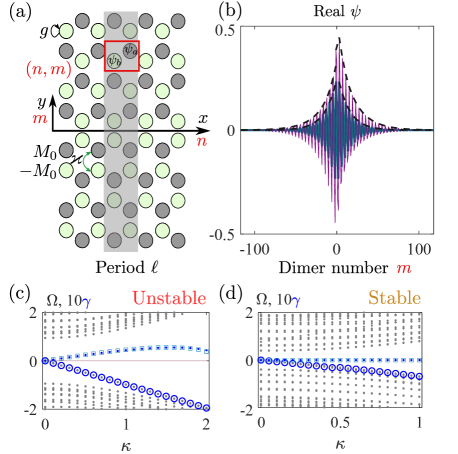
Given that staggered graphene Ni2018 ; RingSoliton2018 ; smirnova2019topological ; Smirnova2020LiSA ; smirnova2021gradient can be well-described by the NDM Eq. (1) in the continuum limit, we will use a dimerized honeycomb lattice for further validation of our results with the example of a discrete two-dimensional system made of coupled sites. We consider the ribbon geometry of the lattice, which is periodic along the horizontal () direction and has a finite size in the vertical () direction and utilize the tight-binding equations governing the propagation dynamics, which assumes that each element is subject to linear interactions with the coupling coefficient with its’ three nearest neighbours only:
| (8a) | |||
| (8b) | |||
where a pair of integers enumerates the dimer along (as ) and (as ) directions [see Fig. 3(a)], indices distinguish two different sublattices, and we introduced the local on-site nonlinerity of the strength . We consider the periodic stripe along -direction, implying that the steady solution has the form . The period is chosen such that the Dirac velocity, being the coefficient in front of the first derivative, in the corresponding continuum NDM Eq. (1), is unity. In fact, NDM (1) can readily be derived from the system (8) by expanding the Hamiltonian near the high-symmetry point Ni2018 ; Smirnova2020LiSA , and, following this procedure, the dispersion coefficient is .
We search for the solution of system (8) in the form
| (9) |
where the wavefunction represents the precise shape of the nonlinear Dirac edge mode [see Fig. 3 (b)], which can be numerically obtained using Newton’s method. On the other hand, are small disturbances of the edge mode. Similar to Sec. II, we examine the eigenvalue spectra of the plane-wave-like perturbations expressed as . The results summarised in Fig. 3 (c,d) are fully consistent with our findings in Sec. II, signalling the presence of the nonlinear correction in MNSE.
IV IV. Optical implementation
The discussed model can potentially be implemented in a range of settings, including optical lattices and metamaterials. In this section, as a possible experimental platform, we examine valley-Hall waveguide arrays made of laser-written single-mode waveguides with parameters similar to those utilized in the experimental work Ref. Noh2018 . The designed photonic lattice can be well described by the tight-binding model with effective parameters and . To study the evolution dynamics in the realistic array, we apply numerical techniques to solve Maxwell’s wave equations in the paraxial approximation, namely, plane wave expansion to get the edge mode profile transverse to the interface and the beam propagation method to simulate propagation.
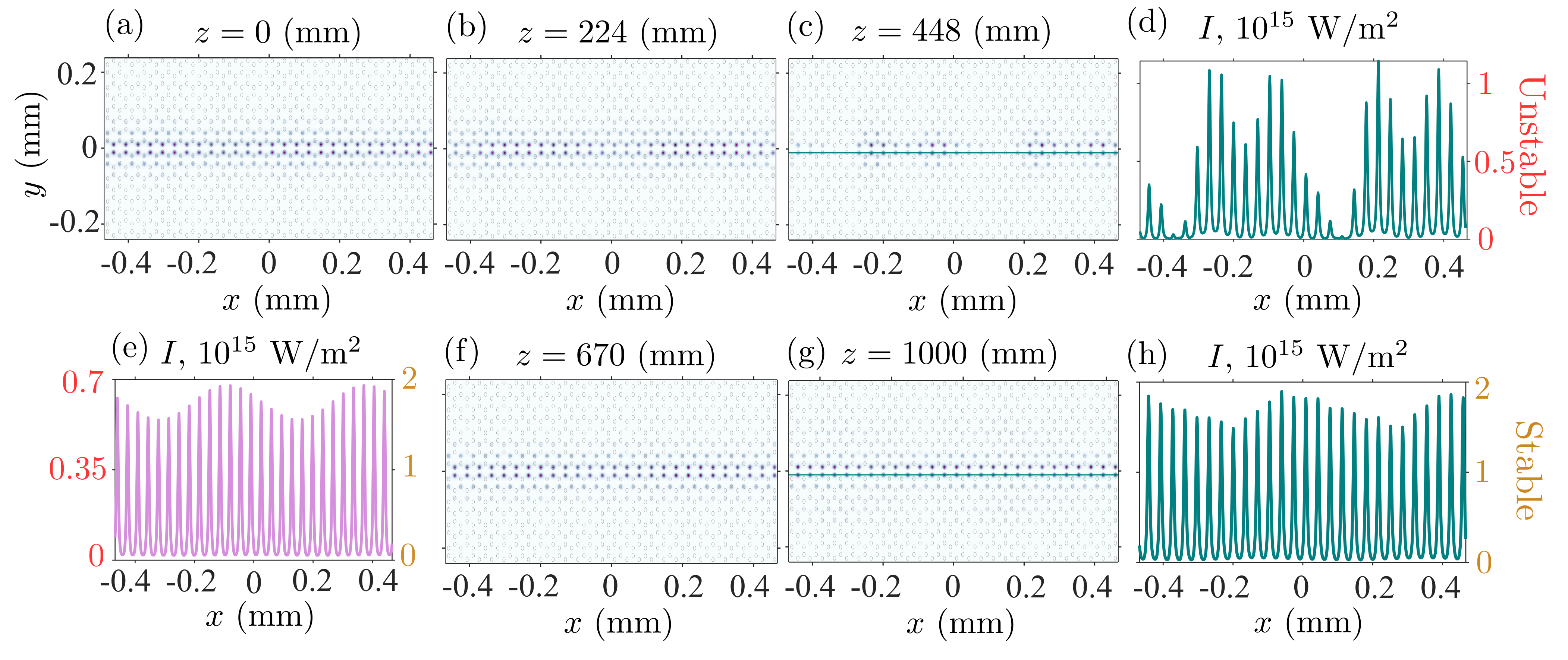
As an initial condition, we set the plane-wave-like edge mode, whose amplitude is perturbed by 5% large-scale noise [see Figs. 4(a,e)]. Then we directly model its dynamics up to large propagation distances along axis, being the evolution coordinate analogous to variable in Eq. (1), for the two different wave amplitudes falling into the unstable and stable regions in the parameter space for comparison. Representative snapshots of instability development are shown in Figs. 4 (b,c,d). The unstable edge state disintegrates into a series of soliton-like localized distributions. On the contrary, in Figs. 4(f,g,h) we observe that the perturbed edge mode remains unchanged up to large distances, thereby indicating the stabilization effect. Note, however, apart from the perturbations localized near the domain wall and well described by Eq. (2), the amplitude of the nonlinear wave in a realistic lattice can also undergo fluctuations caused by the bulk perturbations or coupling with other interfaces. This can shift a transition towards either the unstable or stable regime.
V Conclusion
The performed study emphasises the importance of the nonlinear velocity term in the modified nonlinear Schrödinger equation for the adequate effective description of the nonlinear dynamics of edge waves supported by topological interfaces in the long-wavelength limit. As its’ subtle consequence, the effect of the nonlinear edge mode stabilization at the valley-Hall interfaces was confirmed by the linearized stability analysis and direct dynamic modeling. Given the generality of the models and methods employed, our results establish the useful analytic concept of intuition for understanding dynamic effects in nonlinear topological photonic systems of various nature.
VI Acknowledgements
E.S. and L.S. are supported in part by the MSHE under project No. 0729-2021-013. E.S. thanks the Foundation for the Advancement of Theoretical Physics and Mathematics "BASIS" (Grant No. 22-1-5-80-1). D.L. acknowledges support from the National Research Foundation, Singapore and A*STAR under its CQT Bridging Grant. D.S. acknowledges support from the Australian Research Council (DE190100430, CE200100010) and the Japan Society for the Promotion of Science under the Postdoctoral Fellowship Program for Foreign Researchers.
References
- (1) T. Ozawa, H. M. Price, A. Amo, N. Goldman, M. Hafezi, L. Lu, M. C. Rechtsman, D. Schuster, J. Simon, O. Zilberberg, and I. Carusotto, ‘‘Topological photonics,’’ Rev. Mod. Phys. 91, 015006 (2019).
- (2) D. Smirnova, D. Leykam, Y. Chong, and Y. Kivshar, ‘‘Nonlinear topological photonics,’’ Applied Physics Reviews 7, 021306 (2020).
- (3) D. Leykam, E. Smolina, A. Maluckov, S. Flach, and D. A. Smirnova, ‘‘Probing band topology using modulational instability,’’ Physical Review Letters 126, 073901 (2021).
- (4) A. Maluckov, E. Smolina, D. Leykam, S. Gündoğdu, D. G. Angelakis, and D. A. Smirnova, ‘‘Nonlinear signatures of Floquet band topology,’’ Physical Review B 105, 115133 (2022).
- (5) A. Mancic, D. Leykam, and A. Maluckov, ‘‘Band relaxation triggered by modulational instability in topological photonic lattices,’’ Physica Scripta (2023).
- (6) Y. Lumer, M. C. Rechtsman, Y. Plotnik, and M. Segev, ‘‘Instability of bosonic topological edge states in the presence of interactions,’’ Physical Review A 94, 021801 (2016).
- (7) Y. V. Kartashov and D. V. Skryabin, ‘‘Modulational instability and solitary waves in polariton topological insulators,’’ Optica 3, 1228–1236 (2016).
- (8) Y. Zhang, Y. V. Kartashov, and A. Ferrando, ‘‘Interface states in polariton topological insulators,’’ Physical Review A 99, 053836 (2019).
- (9) D. A. Smirnova, L. A. Smirnov, E. O. Smolina, D. G. Angelakis, and D. Leykam, ‘‘Gradient catastrophe of nonlinear photonic valley-Hall edge pulses,’’ Physical Review Research 3, 043027 (2021).
- (10) L. J. Maczewsky, M. Heinrich, M. Kremer, S. K. Ivanov, M. Ehrhardt, F. Martinez, Y. V. Kartashov, V. V. Konotop, L. Torner, D. Bauer, and A. Szameit, ‘‘Nonlinearity-induced photonic topological insulator,’’ Science 370, 701–704 (2020).
- (11) S. Mukherjee and M. C. Rechtsman, ‘‘Observation of Floquet solitons in a topological bandgap,’’ Science 368, 856–859 (2020).
- (12) S. Mukherjee and M. C. Rechtsman, ‘‘Observation of unidirectional solitonlike edge states in nonlinear floquet topological insulators,’’ Phys. Rev. X 11, 041057 (2021).
- (13) M. Jürgensen, S. Mukherjee, and M. C. Rechtsman, ‘‘Quantized nonlinear Thouless pumping,’’ Nature 596, 63–67 (2021).
- (14) M. Jürgensen, S. Mukherjee, C. Jörg, and M. C. Rechtsman, ‘‘Quantized fractional Thouless pumping of solitons,’’ Nature Physics 19, 420–426 (2023).
- (15) J. Guglielmon and M. C. Rechtsman, ‘‘Broadband topological slow light through higher momentum-space winding,’’ Phys. Rev. Lett. 122, 153904 (2019).
- (16) E. Sauer, J. P. Vasco, and S. Hughes, ‘‘Theory of intrinsic propagation losses in topological edge states of planar photonic crystals,’’ Phys. Rev. Research 2, 043109 (2020).
- (17) G. Arregui, J. Gomis-Bresco, C. M. Sotomayor-Torres, and P. D. Garcia, ‘‘Quantifying the robustness of topological slow light,’’ Phys. Rev. Lett. 126, 027403 (2021).
- (18) C. A. Rosiek, G. Arregui, A. Vladimirova, M. Albrechtsen, B. Vosoughi Lahijani, R. E. Christiansen, and S. Stobbe, ‘‘Observation of strong backscattering in valley-hall photonic topological interface modes,’’ Nature Photonics p. 1 (2023).
- (19) M. J. Ablowitz, C. W. Curtis, and Y. Zhu, ‘‘Localized nonlinear edge states in honeycomb lattices,’’ Phys. Rev. A 88, 013850 (2013).
- (20) M. J. Ablowitz, C. W. Curtis, and Y.-P. Ma, ‘‘Linear and nonlinear traveling edge waves in optical honeycomb lattices,’’ Phys. Rev. A 90, 023813 (2014).
- (21) S. K. Ivanov, Y. V. Kartashov, A. Szameit, L. Torner, and V. V. Konotop, ‘‘Vector topological edge solitons in Floquet insulators,’’ ACS Photonics 7, 735–745 (2020).
- (22) S. K. Ivanov, Y. V. Kartashov, L. J. Maczewsky, A. Szameit, and V. V. Konotop, ‘‘Bragg solitons in topological Floquet insulators,’’ Opt. Lett. 45, 2271–2274 (2020).
- (23) D. Anderson and M. Lisak, ‘‘Nonlinear asymmetric self-phase modulation and self-steepening of pulses in long optical waveguides,’’ Physical Review A 27, 1393 (1983).
- (24) N. C. Panoiu, X. Liu, and R. M. Osgood Jr, ‘‘Self-steepening of ultrashort pulses in silicon photonic nanowires,’’ Optics letters 34, 947–949 (2009).
- (25) J. C. Travers, W. Chang, J. Nold, N. Y. Joly, and P. S. J. Russell, ‘‘Ultrafast nonlinear optics in gas-filled hollow-core photonic crystal fibers,’’ JOSA B 28, A11–A26 (2011).
- (26) C. Husko and P. Colman, ‘‘Giant anomalous self-steepening in photonic crystal waveguides,’’ Physical Review A 92, 013816 (2015).
- (27) D. A. Smirnova, L. A. Smirnov, D. Leykam, and Y. S. Kivshar, ‘‘Topological edge states and gap solitons in the nonlinear Dirac model,’’ Laser & Photonics Reviews 13, 1900223 (2019).
- (28) X. Ni, D. Smirnova, A. Poddubny, D. Leykam, Y. Chong, and A. B. Khanikaev, ‘‘ phase transitions of edge states at symmetric interfaces in non-Hermitian topological insulators,’’ Phys. Rev. B 98, 165129 (2018).
- (29) A. N. Poddubny and D. A. Smirnova, ‘‘Ring Dirac solitons in nonlinear topological systems,’’ Phys. Rev. A 98, 013827 (2018).
- (30) D. Smirnova, A. Tripathi, S. Kruk, M.-S. Hwang, H.-R. Kim, H.-G. Park, and Y. Kivshar, ‘‘Room-temperature lasing from nanophotonic topological cavities,’’ Light: Science & Applications 9 (2020).
- (31) J. Noh, S. Huang, K. P. Chen, and M. C. Rechtsman, ‘‘Observation of photonic topological valley Hall edge states,’’ Phys. Rev. Lett. 120, 063902 (2018).