Entangled embedding variational quantum eigensolver with tensor network ansatz

Abstract

In this paper, we introduce a tensor network (TN) scheme into the entanglement augmentation process of the synergistic optimization framework [arXiv: 2208.13673] by Rudolph et al. to build its process systematically for inhomogeneous systems. Our synergistic first embeds the variational optimal solution of the TN state with the entropic area law, which can be perfectly optimized in conventional (classical) computers, in a quantum variational circuit ansatz inspired by the TN state with the entropic volume law. Next, the framework performs a variational quantum eigensolver (VQE) process with the embedded states as the initial state. We applied the synergistic to the ground state analysis of the all-to-all coupled random transverse-field Ising/XYZ/Heisenberg model, employing the binary multi-scale entanglement renormalization ansatz (MERA) state and branching MERA states as TN states with the entropic area law and volume law, respectively. We then show that the synergistic accelerates VQE calculations in the three models without initial parameter guess of the branching-MERA-inspired ansatz and can avoid a local solution trapped by a standard VQE with the ansatz in the Ising model. Improvement of optimizer for MERA in the all-to-all coupled inhomogeneous systems, enhancement and potential applications of the synergistic are also discussed.

I Introduction

The ground state of quantum many-body systems is essential for understanding quantum phenomena in many-body physics. However, solving quantum many-body problems is generally difficult with conventional (classical) computers because they require the treatment of Hilbert spaces that grow exponentially with increasing the system size of $N$.

To address the limitation in solving the problems, using quantum computers has been attracting attention. Actually, quantum algorithms such as the quantum phase estimation [1], the qubitization [2], and the quantum singular value transformation [3] with quantum acceleration, unable us to access the ground state for large quantum many-body systems that intractable for classical computers.

However, the current quantum computers are noisy intermediate-scale quantum (NISQ) devices[4], which suffer from errors and have limited size. To make them more practical, we need quantum algorithms that can be executed with shallow quantum circuits. In this situation, one of the NISQ-aware methods developed is the Variational Quantum Algorithm (VQA) [5]. This method involves constructing variational models through parameterized quantum circuits (also called ansatz) on a quantum computer and then optimizing the cost function using classical computers. VQAs, specifically the variational quantum eigensolver (VQE), have been applied to search for the ground state of quantum systems.[6].

To obtain meaningful results using VQAs on NISQ, the ansatz used to represent the target state with the required precision should have few internal parameters and as shallow as possible in terms of circuit depth. This condition is essential to mitigate the noise effects specific to NISQ devices and avoid the occurrence of the barren plateau (BP) problem[7] associated with excessive variational space. Although the BP problem can be circumvented by starting the calculation from appropriate initial parameters[8], it is generally non-trivial to set such parameters. Therefore, a systematic procedure for setting up high-quality ansatz is strongly desired.

As one strategy to satisfy this requirement, procedures of putting more classical-computer resources in a series of processes of VQE are currently attracting attention [9, 10]. Especially the VQE with a synergistic framework [10] is a quantum-classical hybrid algorithm that has received much attention to avoid BP problems. The synergistic framework has two key concepts: sophisticated variational methods on classical computers perfectly give the initial state for the VQE, and the quantum gates added during the VQE calculation and the quantum circuit in which the classically optimized solution is efficiently embedded have different topologies. This second concept is referred to as the entanglement augmentation process.

The use of the tensor network (TN) method [11, 12, 13, 14] for the first concept of the synergy framework is a natural idea since the TN method for quantum states represents the wave function as a contraction of many tensors with small degrees of freedom (TN representation) and is a way to realize the variational method of large quantum many-body systems on a classical computer; there is an ongoing effort to convert TN states into quantum circuits representation today [15, 16, 17].

Actually, in Ref. [10], the authors used the matrix product state (MPS) [18, 19, 20], which has one-dimensional (1D) topology, as variational methods on classical computers, and employed all-to-all topologies of fully parametrized SU(4) gates for the augmentation process. However, as mentioned in Ref [10], constructing the all-to-all topology is a nontrivial task and is likely not scalable on NISQ devices. Therefore, to achieve a synergistic framework irrespective of the task and can be implemented on near-to-mid-term quantum computers, it is necessary to propose a systematic entanglement augmentation process that can qualitatively and dramatically change the entanglement structure of the ansatz by only adding a very sparsely coupled quantum gates.

In this paper, we introduce the concept of TN structure into this entanglement augmentation process and propose a procedure to efficiently and systematically augment the entanglement representation capability of quantum circuit ansatz. Specifically, we focus on embedding a TN state with entropic area law [21] after variational calculation on the classical computer in a portion of the entanglement-augmented quantum circuit ansatz that is equivalent to a TN state with the entropic volume law. This entangled embedding VQE (EEVQE) approach can accelerate the calculations of VQE with TN-inspired ansatz with entropic-volume-law. Discussions of embedding focused on TN with the entropic volume law and its connection to VQE, which is an attempt not seen in the pioneering works [22, 17] related to our study. Investigations of TN state with the entropic volume law are important for analyzing the quantum states in complex problems, such as quantum chemical systems, long-range interacting systems, random spin systems that involve non-uniform interactions among all qubits, and simulations of real-time evolution for quantum systems because the quantum states may not satisfy the entropic area law in these systems. For specific numerical verification of EEVQE, we employ 1D binary multi-scale entanglement renormalization ansatz (MERA) [23, 24] for variational method on a classical computer and use branching MERA networks [25, 26] as quantum circuit ansatz after entanglement augmentation. The target Hamiltonians are all-to-all coupled random transverse-field Ising/XYZ/Heisenberg models whose ground states can violate the entropic area law. As we expect, through the EEVQE process, we confirm for three models that TN states after the variational optimization on classical computers can be further improved in terms of variational energy while benefiting from the initialization-problem-free and accelerating VQE calculations. Furthermore, we also confirm that EEVQE can avoid traps to locally optimal solutions (or broadly BP) in the random transverse field Ising model.

As part of our efforts to advance the synergistic framework, we performed a detailed comparison of optimizers to update MERA for all-to-all coupled random systems. This involved comparing the Evenbly-Vidal method [24], the standard in MERA optimization, its improvements developed in this work (refer to Sec. III.2), and the Broyden-Fletcher-Goldfarb-Shanno (BFGS) method, which is the standard in parameterized quantum circuit ansatz optimization. Our comparison results showed that the BFGS method was the most effective in reducing the variational energy for all the models we studied. This result indicates the importance of introducing the knowledge of optimizer often used in VQE to accelerate the computation of variational methods with TN on the classical computer in the application of the synergistic framework to investigate low-energy states of quantum chemical calculations, which is the most desired application of VQE for all-coupled inhomogeneous systems.

The remainder of the paper is organized as follows: in Sec. II, we review the basics of the components of EEVQE, namely TN structures of MERA and branching MERA, Evenbly-Vidal sequential optimization method, VQE and the synergistic framework; in Sec. III, we describe our propositions, i.e., the procedure of embedding MERA states into quantum circuit ansatz inspired by branching MERA states and the procedure of a modified Evenbly-Vidal method; in Sec. IV, after investigating the performance of optimizers for MERA states in a specific set of all-to-all coupled models, we present the results of a performance study of EEVQE for the models. Finally, in Sec. V, we summarize the paper and discuss the future studies of EEVQE.

II Reviews for components of EEVQE

In this section, we review the fundamentals of the components of EEVQE: the TN structures of 1D binary MERA and branching MERA, optimization methods for MERA, the calculation procedure of VQE, and the synergistic framework. One familiar with these components may skip to the next section, which discusses how to embed the optimized MERA state in branching-MERA-inspired quantum circuits and the scrutiny of optimization methods for MERA in the all-to-all coupled model.

II.1 TN structures of 1D binary MERA and branching MERA

Here, let us consider the 1D binary MERA, whose schematic diagram is depicted in Fig. 1(a).

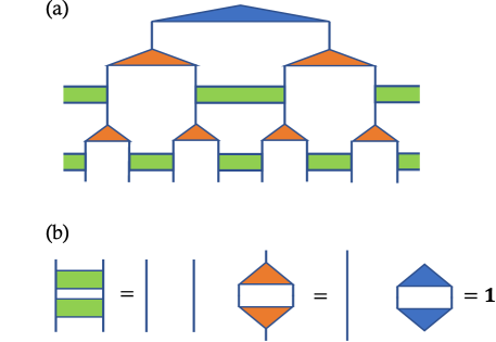
Figure 1: Schematic diagrams of (a) the binary MERA for the 8-site system and (b) isometric conditions of disentangler, isometry, and top tensors.

The binary MERA network for finite-size systems consists of fourth-, third-, and second-order tensors called disentanglers $u$, isometries $w$, and top tensors $t$ (see Fig. 1). In the following, to simplify the discussion, the degrees of freedom (bond dimension) of each leg of all tensors are assumed to be a common positive integer $\chi$ (See the original paper in MERA [24] for an extension of the discussion to the case where the bond dimension is tensor dependent). Each $u$, $w$, and $t$ on the network always satisfies the following orthonormality or isometric conditions

$$\sum_{cd}\left(u^{ab}_{cd}\right)^{*}u^{a^{\prime}b^{\prime}}_{cd} = \delta_{aa^{\prime}}\delta_{bb^{\prime}},$$ (1)

$$\sum_{ab}\left(u^{ab}_{cd}\right)^{*}u^{ab}_{c^{\prime}d^{\prime}} = \delta_{cc^{\prime}}\delta_{dd^{\prime}},$$ (2)

$$\sum_{ab}\left(w^{c}_{ab}\right)^{*}w^{c^{\prime}}_{ab} = \delta_{cc^{\prime}},$$ (3)

$$\sum_{ab}\left(t_{ab}\right)^{*}t_{ab} = 1~{},$$ (4)

where $\delta_{\alpha\alpha^{\prime}}$ with $\alpha\in\{a,b,c,d\}$ is the Kronecker delta. These conditions are schematically shown in Fig. 1(b). Thanks to the conditions, the quantum state $\ket{\Psi}$ represented by MERA is always normalized, namely $\innerproduct{\Psi}{\Psi}=1$. This paper considers position-dependent TN, where each tensor has different tensor elements depending on its placement on the network.

To achieve a wider variational space, the 1D branching binary MERA in Fig. 2 introduces a branching structure into isometry while keeping layer structures of the MERA. In the case of the branching binary MERA, the orthonormality of the isometry in which the bifurcation is introduced is identical to that of the disentangler $u$. Since the branching structure can be arbitrarily introduced in each isometry layer in the binary MERA as shown in Fig. 2, variations of $2^{n-1}$-pattern branching structures are possible in a $2^{n}$-site system.

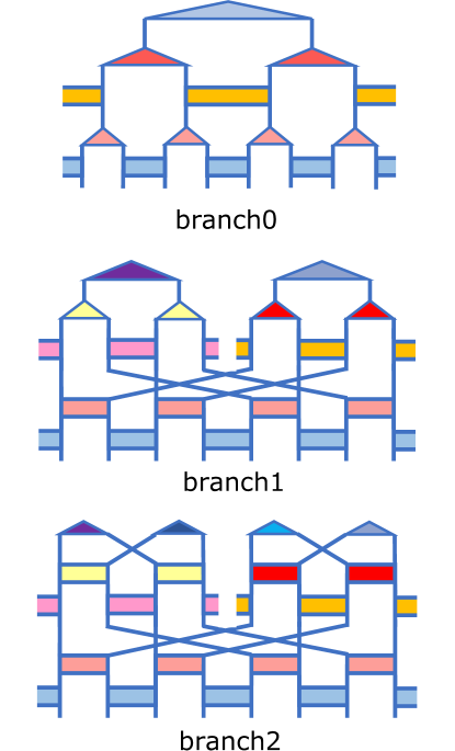
Figure 2: Pattern diagram of the binary MERA to the branching MERA in an 8-site system. Since branches can be added at each layer, we name the diagram to branch0, branch1, branch2,$\dots$ for each number of branches.

This paper focuses only on a full-branching MERA, which introduces branching in all isometry layers, for example, branch 2 in Fig. 2.

II.2 Optimization scheme for MERA

This subsection offers the Evenbly-Vidal algorithm, which is used as standard optimization of MERA. Given the Hamiltonian $\mathcal{H}$ of the targeted system, the variational energy $E$ can be evaluated in $\expectationvalue{\mathcal{H}}{\Psi}$, where $\ket{\Psi}$ is the variational state in terms of the binary MERA. We consider now that the Hamiltonian consists of the sum of two-body interactions $h_{ij}$ between $i$- and $j$-th sites, namely $\mathcal{H}=\sum_{i<j}h_{ij}$. In this case, the expectation value of each interaction $e_{ij}=\expectationvalue{h_{ij}}{\Psi}$ can be summed to obtain the variational energy $E$. For practical calculations, we should perform the minimum contraction, which depends on the $(i,j)$-pairs by utilizing the isometric condition of $u,w,t$, or causal cone as shown in Fig 3, and the typical computational cost of evaluating $e_{ij}$ is known to be $O(\chi^{9}\log N)$ if the system size is large enough [24]. For example, given a MERA, suppose we want to optimize an isometry $w$ while keeping the rest of the tensors fixed. The energy $E$ depends quadratically on $w$ and $w^{{\dagger}}$, namely

$$E(w)=\sum_{abca^{\prime}b^{\prime}c^{\prime}}\sum_{\langle i<j\rangle}\left(w^{c}_{ab}\right)^{*}\left[\mathcal{E}_{ij}\right]^{abc}_{a^{\prime}b^{\prime}c^{\prime}}w^{c^{\prime}}_{a^{\prime}b^{\prime}}+C$$ (5)

where $\langle i<j\rangle$ refers to the set of site pairs specifying the two-body pair interaction $h_{ij}$ that contributes to the optimization of $w$, and $\mathcal{E}_{ij}$ is the environment tensor obtained by hollowing out the diagrams corresponding to $w$ and $w^{{\dagger}}$ from the causal cone necessary to evaluate $e_{ij}$ [24], and $C=\sum_{\overline{\langle i<j\rangle}}e_{ij}$ with $\sum_{i<j}=\sum_{\langle i<j\rangle}+\sum_{\overline{\langle i<j\rangle}}$ is a constant term with respect to the update of $w$.

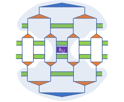
Figure 3: Schematic diagram of $e_{ij}$ with $(i,j)=4,5$, and the light-shaded region shows the causal cone structures. Diagrams outside the causal cone are trivially simplified to the identity operator by the isometric condition.

No known algorithm exists to solve a quadratic problem keeping the isometric constraint.

Evenbly and Vidal developed how to optimize a single tensor of the MERA based on a linearizing approximation [24]. In this approach, we temporally regard $w$ and $w^{{\dagger}}$ as independent tensors and optimize $w$ while keeping $w^{{\dagger}}$ fixed, namely

$$\tilde{E}(w) \equiv \sum_{abc}\left[\Upsilon_{w}\right]^{c}_{ab}w^{c}_{ab}~{},$$ (6)

$$\left[\Upsilon_{w}\right]^{c^{\prime}}_{a^{\prime}b^{\prime}} \equiv \sum_{abc}\sum_{\langle i<j\rangle}\left(w^{c}_{ab}\right)^{*}\left[\mathcal{E}_{ij}\right]^{abc}_{a^{\prime}b^{\prime}c^{\prime}}~{},$$ (7)

where the tensor $\Upsilon_{w}$ is called the environment tensor of the $w$. To achieve a unique global minimization of $\tilde{E}(w)$, a singular value decomposition (SVD)

$$\left[\Upsilon_{w}\right]^{c}_{ab}\stackrel{{\scriptstyle\rm{SVD}}}{{=}}\sum_{c^{\prime}}V_{cc^{\prime}}S_{c^{\prime}}W^{*}_{c^{\prime}ab}$$ (8)

is performed on the environment tensor. The tensor $w_{\text{new}}$ that minimizes $\tilde{E}(w_{\text{new}})$ is always given by

$$\left[w_{\text{new}}\right]^{c}_{ab}=-\sum_{c^{\prime}}V^{*}_{cc^{\prime}}W_{c^{\prime}ab}~{}.$$ (9)

For this update to always work well, the Hamiltonian should be redefined as $\mathcal{H}_{\gamma}=\mathcal{H}-\gamma I$ with $\gamma$ sufficiently large to $\mathcal{H}_{\gamma}$ is negative definite. However, the optimization step size is scaled by $\gamma^{-1}$ [27], so we should choose $\gamma$ as small as possible practically. In the Evenbly-Vidal method in non-uniform MERA, this linearized update is performed sequentially for each tensor constructing MERA.

In the same manner, we can obtain $e_{ij}$ and optimize TN with the branching binary MERA; the typical numerical cost of evaluating $e_{ij}$ is reported to be $O(\chi^{12}N)$ if the system size is large enough [25]. Compared to the computational cost of MERA, the cost of the branching MERA is extremely large, which has been the primary factor that has kept us away from analyzing the performance of branching MERA with classical computers.

II.3 Variational Quantum Eigensolver

The variational quantum eigensolver (VQE) [6] is a quantum-classical hybrid variational method for finding the ground state energy of a target Hamiltonian $\mathcal{H}$ on an $N$-qubit system. In the VQE, the variational wave function for the system is expressed as a product of parameterized quantum unitary gates

$$\ket{\Psi({\bm{\theta}})}=\prod_{k=1}^{K}\hat{u}_{k}(\bm{\theta}_{k})\ket{0}^{\otimes N},$$ (10)

where $\bm{\theta}=(\bm{\theta}_{1},\bm{\theta}_{2},\cdots,\bm{\theta}_{K})$ and $\hat{u}_{k}(\bm{\theta}_{k})$ means $k$-th quantum gate acting on single or multiple qubits specified by the user and has variational parameters $\bm{\theta}_{k}=(\theta_{k,1},\theta_{k,2},\cdots,\theta_{k,\ell_{k}})$; $\ell_{k}$ is the number of internal degree of freedom for $\hat{u}_{k}$. In this paper, each $\hat{u}_{k}$ is an SU(4) gate, where $\bm{\theta}_{k}$ becomes a 15-dimensional real vector, acting on the $i_{k}$-th and $j_{k}$-th qubits with $1\leq i_{k}<j_{k}\leq N$. The variational wave function $\ket{\Psi}$ is always normalized due to the unitarity of the gates.

A goal of VQE is to minimize the variational energy

$$E = \min_{\bm{\theta}}E(\bm{\theta}),$$ (11)

$$\textrm{where}~{}~{}E(\bm{\theta}) = \expectationvalue{\mathcal{H}}{\Psi({\bm{\theta}})}$$

with respect to $\bm{\theta}$. Since numerically exact values of the partial derivatives

$$\left\{\partial_{\theta_{k,l}}E(\bm{\theta})=\frac{E(\bm{\theta}+\frac{\pi}{2}\bm{e}_{k,l})-E(\bm{\theta}-\frac{\pi}{2}\bm{e}_{k,l})}{2}\right\}^{1\leq k\leq K}_{1\leq l\leq\ell_{k}}$$ (12)

with the orthonormal unit vector $\bm{e}_{k,l}$ for shifting only the parameter $\theta_{k,l}$ are easily obtained by the parameter shift rule [28], we can employ various gradient-based algorithms as optimizers of the VQE. In VQE, the calculation of expectation values $\{E(\bm{\theta}),E(\bm{\theta}\pm\frac{\pi}{2}\bm{e}_{k,l})\}$ is performed on a quantum computer since the calculation is a bottleneck in simulations using classical computers. Then, the classical computer updates the parameters using the gradient $\nabla E(\bm{\theta})$. Of course, you may choose an optimizer that does not use the gradient or uses the Hessian, which can be also evaluated by the parameter shift rules. Finally, VQE achieves the ground state search by iterative calculations between the procedures of classical and quantum computers.

The hyperparameters of the VQE are the initial values of the variational parameters, including the design of the quantum gate set, the choice of the optimizer, and the hyperparameters that the optimizer has (See the review [29] for more information). These hyperparameters should be properly controlled according to the quantum computer’s ability for high-precision calculations in VQE. In particular, when using NISQ devices, it is important to attempt to decrease the total number of quantum gates used within an acceptable range of numerical accuracy to reduce the effect of noise.

II.4 The synergistic framework

The problem with VQAs in NISQ devices is that statistical and systematic errors are associated with the measurement and noise, respectively. A naive approach to solving the problem is a policy of reducing the dependence on NISQ devices in existing quantum-classical hybrid algorithms. For example, Okada et al. proposed an efficient protocol for topological phase analysis of transverse field cluster and toric code models on quantum circuits[9]. In this protocol, all the optimization of the quantum circuit, including the calculation of expectation values, is performed on a classical computer using causal cone structures, as discussed in Fig. 3 for each local observable. In addition, the expectation value evaluation of non-local observables, which are difficult to handle on a classical computer, is performed using the classically optimized quantum circuit.

However, this protocol has constraints on the target system and ansatz. For example, measured observables used in optimization are local, and ansatz is composed of local gates and has constant depth. To avoid this difficulty, first, the synergistic framework in Ref. [10] employs the MPS after the variational calculation with TN methods on the classical computer and performs quantum circuit encoding of the MPS by sequential two-qubit-gate decomposition with 1D topology [30, 31] as the initial ansatz of the VQE. Second, the framework augments the quantum circuit encoded from the MPS with an additional parameterized quantum circuit. In this step, the internal parameters of the additional quantum circuit are all set to zero so that they correspond to identity operators. Finally, the framework performs VQE with the augmented circuit as the initial ansatz. The important properties of the framework can be summarized in the following two points: the VQE is trapped in the BP when all parameters of augmented ansatz are given randomly but can avoid the BP by use of the encoded quantum circuit; the all-to-all gate topology, which is different from the topology of the MPS, of the quantum circuit added after the quantum circuit encoding effectively contributes to better VQE performance. These importances are also noted in Ref. [16].

It is worth noting that in Ref. [10] of the synergistic framework, the SU(4) gate product is created through a sequential process during the quantum-circuit encoding of the MPS. This process makes it difficult to fully utilize classical computing power as a divide-and-conquer approach cannot be naively introduced. Additionally, while all-to-all topology gates are the most commonly used for entanglement augmentation, it is not a systematic procedure. To achieve a quantum advantage in non-uniform systems like quantum chemical systems by the synergistic framework, TN states that can be easily converted to quantum circuits must be introduced. Sparse gates should also be added during the entanglement augmentation process, which requires a significant change in the entanglement structure of the variational quantum state.

III Entangled embedding VQE

To this end, we propose a protocol, called entangled embedding VQE (EEVQE), using binary MERA for classical variational optimization and branching MERA augmented from binary MERA on a quantum circuit. It can be summarized in four steps:

1. Perform the variational optimization of the MERA state with entropic area law on the classical computer for the target Hamiltonian.

2. Obtain the quantum circuit representation of the optimized MERA state using the technique of quantum circuit encoding.

3. Embed the encoded circuit to an entanglement-augmented quantum circuit inspired by the branching MERA state with entropic volume law.

4. Perform the VQE with the initial state given by the augmented circuit.

The following subsection will explain how to incorporate MERA states into a quantum circuit ansatz with the same degrees of freedom as the branching MERA state. Additionally, we will introduce a modified version of the Evenbly-Vidal technique for updating MERA during classical variational optimization. This will be used to compare optimizers for updating MERA in all-to-all coupled random systems, as discussed in Sec. IV.2.

III.1 Quantum circuit representation of MERA and embedding process

The disentangler $u$, isometry $w$, and top tensor $t$ with the bond dimension $\chi=2^{n}$ of MERA equivalent to the SU($2^{2n}$) rotation operator ($2n$-qubit gate) have different condition of input qubits $\ket{0}^{\otimes n}$ states as shown in Fig. 4(a). We depict quantum circuit representations of the binary MERA and branching MERA according to the above rule in Fig. 4(b).

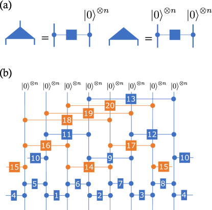
Figure 4: Schematic diagrams of (a) quantum circuit representations of disentangler, isometry, and top tensors, and (b) quantum circuit representation of the branching MERA for $N=8n$ with $\chi=2^{n}$ consisting 20 SU($2^{2n}$) $2n$-qubit gates, where blue diagrams mean the degree of freedom of (non-branching) MERA.

One of the processes of embedding the isometry and top tensors elements, which form the MERA state after variational optimization on a classical computer, into a unitary matrix of SU($2^{2n}$) involves using the modified Gram-Schmidt method (See Appendix. A).

In the case of $n=1$, by use of Cartan decomposition, any SU(4) operator $\hat{u}_{ij}$ for $i$- and $j$-th qubits can be decomposed into a kind of time evolution operator $\mathcal{D}_{ij}$ with XYZ-type interaction and SU(2) rotation operators $\mathcal{R}_{i}$ for one qubit [32], that means $u_{ij}=\mathcal{R}_{i}\mathcal{R}_{j}\mathcal{D}_{ij}\mathcal{R}^{\prime}_{i}\mathcal{R}^{\prime}_{j}$ where

$$\mathcal{D}_{ij}=e^{-{\rm i}{\bm{k}}\cdot{\bm{\Sigma}}_{ij}},~{}\mathcal{R}_{i}=e^{-{\rm i}\psi\sigma^{z}_{i}/2}e^{-{\rm i}\theta\sigma^{y}_{i}/2}e^{-{\rm i}\phi\sigma^{z}_{i}/2}$$ (13)

with ${\bm{k}}=(k^{x},k^{y},k^{z})$, ${\bm{\Sigma}}_{ij}=(\sigma_{i}^{x}\sigma_{j}^{x},\sigma_{i}^{y}\sigma_{j}^{y},\sigma_{i}^{z}\sigma_{j}^{z})$; ${\bm{\sigma}}_{i}=(\sigma_{i}^{x},\sigma_{i}^{y},\sigma_{i}^{z})$ is the Pauli operator for $i$-th qubit.

To execute $2n$-qubit gates equivalent to the unitary matrix on a quantum computer, decomposing the $2n$-qubit gates into a product of two-qubit SU(4) gates is essential because once we have the product, we can break down each SU(4) gate into CNOT gates and single-qubit rotational gates [33], which are commonly used in NISQ today. Computer-assisted search and numerical optimization for the circuit decomposition have been widely studied [34, 35, 36, 37, 38, 39, 40, 41, 42, 43, 44, 45]. We can encode the MERA state in a quantum circuit by using decomposition techniques on each SU($2^{2n}$) gate individually and simultaneously on classical parallel computing.

To explain the embedding process in detail, we refer to Fig. 4(b), wherein the MERA state is embedded through quantum gates within the blue gate. The branching MERA is represented by a quantum circuit that has an additional orange quantum gate alongside the blue gate. The embedding process is accomplished by setting the internal parameters such that all orange circuits function as identity operators. In case the VQE calculation, with the circuit as the initial condition, gets stuck in a local solution, we introduce weak noise to the orange (and/or blue) quantum gates to avoid such a situation [10, 16].

Studying the effectiveness of branching MERA through quantum computer degrees of freedom is a beneficial approach as it entails lower computational costs in comparison to MERA simulations on a classical computer. MERA requires an order of SU($2^{2n}$) gates of $O(N)$ while branching MERA requires $O(N\log N)$. These costs refer to the computational requirements for producing a quantum state in a quantum computer by operating quantum gates on individual qubits. However, if the computer can compute mutually commutative quantum gates that are spatially separated, both computational costs can be reduced to $O(\log N)$, which corresponds to the number of layers of isometry and disentangler. As a result, the relative computational cost of branching MERA becomes similar to that of MERA.

III.2 Improved Procedures for Sequential Tensor Optimization in MERA

Since the main focus of this study is on applications to all-to-all coupled random systems, the classical computational part of the optimization of the inhomogeneous MERA becomes important and nontrivial. To handle this situation, we modify the optimization method (Evenbly-Vidal method) employed in the original paper [24]. This procedure updates the tensor to be optimized by using the singular vector obtained by singular value decomposition of the environment tensor constructed by all tensor contractions except the tensor to be optimized. However, a huge number of sweep optimizations must be performed with this method, even for MERA networks with enough bond dimension $\chi$ to represent the ground state of the target system, reflecting the effect of linearizing the tensor optimization.

An approach to reduce the number would be to perform diagonalization of the effective Hamiltonian without linearizing the cost function with respect to only the top tensor of the MERA network. The top tensor in the MERA network corresponds to the quantum circuits labeled by number 13 in Fig. 4(b).

Here, we suppose that the total Hamiltonian $\mathcal{H}=\sum_{i<j}h_{ij}$ is given by the sum of two-body Hamiltonian $h_{ij}$ between $i$- and $j$-th sites. Then the effective Hamiltonian $\mathcal{H}^{\prime}$ needed to optimize circuit 13 can likewise be given by the sum of local two-body effective Hamiltonian $h^{\prime}_{ij}$. Diagrammatic representation of the matrix element of $h^{\prime}_{ij}$, namely

$$h^{\prime(ij)}_{mn,m^{\prime}n^{\prime}}=\matrixelement{m,n}{h^{\prime}_{ij}}{m^{\prime},n^{\prime}}~{},$$ (14)

with $0\leq m,n<\chi$ is shown in Fig. 5, where we use the MERA network of Fig. 4(b) for the variational state. After the contractions, we perform the diagonalization on the effective Hamiltonian $\mathcal{H}^{\prime}$ and the eigenvectors $\{\Psi^{\prime}_{mn}\}$ corresponding to the ground states of $\mathcal{H}^{\prime}$ are computed. Finally, the update of circuit 13 is completed by embedding

$$\left(u^{(13)}\right)^{0,0}_{mn}:=\Psi^{\prime}_{mn}$$ (15)

and performing the unitarization as noted in Sec. III.1.

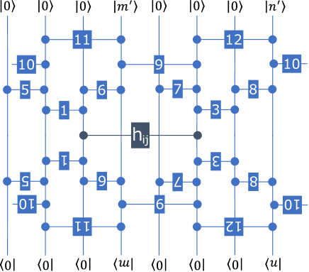
Figure 5: Diagrammatic representation of an effective local two-body Hamiltonian $h^{\prime(ij)}_{mn,m^{\prime}n^{\prime}}$ for the MERA as in Fig. 4(b) with $(i,j)=(3,6)$ and $\chi=2$. The quantum circuits labeled with numbers 2 and 4 are omitted because they do not contribute to the effective local Hamiltonian at all.

It should be mentioned here that such embedding of eigenvectors obtained by the diagonalization of the effective Hamiltonian into the tensor to be optimized is difficult to perform for tensors other than the top tensor because the MERA network, unlike the tree tensor network (TTN) [46, 47, 48], contains a loop structure. On the other hand, the diagonalization is applicable to the optimization of parameterized quantum gates that act only on the zero kets of the initial state, regardless of the details of the variational quantum circuit ansatz.

IV Numerical simulations

IV.1 Hamiltonians and numerical setup

In order to investigate the properties of our procedure, we consider the following all-to-all coupled random transverse field Ising model

$$H_{\textrm{Ising}}=\sum_{i<j}{J_{ij}\sigma^{z}_{i}\sigma^{z}_{j}}+\sum_{i}{h_{i}\sigma^{x}_{i}}~{},$$ (16)

XYZ model

$$H_{\textrm{XYZ}}=\sum_{i<j}{\bm{J}}_{ij}\cdot{\bm{\Sigma}}_{ij},$$ (17)

and Heisenberg model in a random field

$$H_{\textrm{Heisenberg}}=\sum_{i<j}J_{ij}\bm{1}\cdot{\bm{\Sigma}}_{ij}+\sum_{i}{\bm{h}}_{i}\cdot{\bm{\sigma}}_{i}$$ (18)

with ${\bm{1}}=(1,1,1)$, where the coupling constants $J_{ij}$, ${\bm{J}}_{ij}=(J^{x}_{ij},J^{y}_{ij},J^{z}_{ij})$ and the magnetic fields $h_{i}$ and ${\bm{h}}_{i}=(h^{x}_{i},h^{y}_{i},h^{z}_{i})$ are given by uniform random numbers in the range [-1,1). In the actual calculation, the Hamiltonians are pre-processed to be negative definite by shifting the constant terms $\gamma_{ij}$, which is defined as $\gamma_{ij}=\max[f_{ij},0]$ with $f_{ij}$ as the maximum eigenvalue of $h_{ij}$, as discussed in Sec. II.2.

The quantity evaluated hereafter is the relative error from the exact ground state energy $E_{\rm exact}$

$$\Delta=(E-E_{\rm exact})/E_{\rm exact}$$ (19)

and its random-averaged values $\bar{\Delta}$, where we prepare $10^{2}$ realizations for the random coupling constants and magnetic fields. Then, the initial parameters of the MERA state in each realization are common random values.

For the variational update of the MERA state on the classical computer, we adopt the modified Evenbly-Vedal method as we discussed in Sec. III.2 to benefit from the TN method on the classical computer (See Sec. IV.2). The sequential update schedule for tensors was set from the bottom layer to the top layer in the diagram of Fig. 1(a), adopting a left-to-right order within each layer, and the number of iterations for the sequential update is up to $10^{3}$. In this study, we use the Julia version of the ITensors library [49] for TN calculations and only consider $\chi=2$ to focus on the exact circuit encoding of the MERA state.

Then, we use the quantum-simulation software called Cirq [50] for the quantum circuit encoding of SU(4) unitary matrix by use of the Cartan’s decomposition. Note that the decomposition of MPS[30, 31], which does not inherently guarantee unitarity, is a sequential process, while the MERA network proposed in this study is composed of tensors that satisfy unitarity, so it can be easily parallelized because it targets one-unitary decompositions independent of its structure. VQE procedure employs the BFGS method, a type of quasi-Newtonian method. The hyperparameter is only the number of BFGS iterations in this step, and the number is taken up to $10^{4}$ in our study.

In this paper, we focus on how well the VQE calculation of branching MERA with the optimized MERA as the initial wave function performs when the effect of noise is not considered, so we utilize a quantum circuit simulator qulacs [51] and the numerical analysis software library scipy [52] for VQE calculations.

IV.2 Bemchmarks of MERA optimization procedure

Since classical optimization of inhomogeneous MERA is important, as mentioned before, we first compare which optimization method performs better in three optimization methods - Evenbly-Vidal, modified Evenbly-Vidal, and BFGS in the random Ising/XYZ model with all-to-all couplings. The results are presented in Fig. 6, where the color lines and the light-shaded region mean $\bar{\Delta}$ and its variance, respectively.

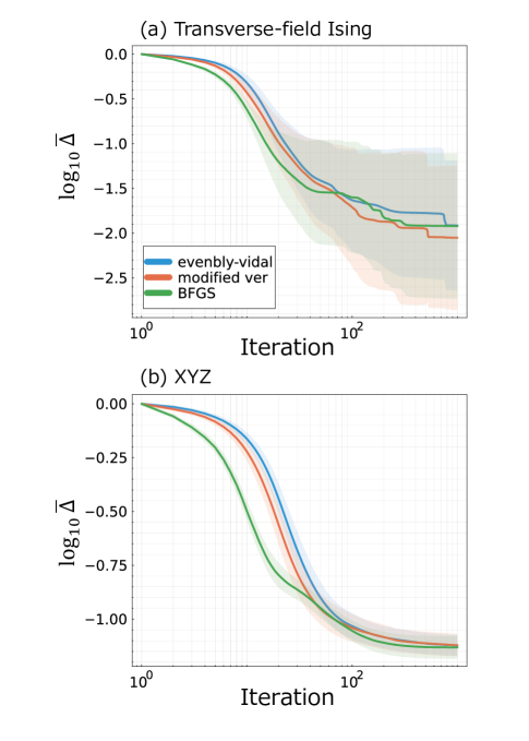
Figure 6: Iteration dependence of $\bar{\Delta}$ for all-to-all coupled random (a) Ising and (b) XYZ systems with $(\chi,N)=(2,16)$.

The results of our study demonstrate that the modified Evenbly-Vidal method exhibits marginally superior convergence speed compared to the original method in both models. Additionally, our findings indicate that the modified method enhances the convergence error in the transverse Ising model. Moreover, we conducted a comparison between the modified Evenbly-Vidal method and the BFGS for the variational optimization of the MERA state. The results show that BFGS is more effective in reducing the variational energy during the initial optimization phase than the modified Evenbly-Vidal method for all models analyzed. It agrees with the expectation that the sequential optimization based on the TN method may be relatively easy to trap in local minima.

Also, we briefly confirm that the performance of the modified Evenbly-Vidal method improves as the weight of the degree of freedom of the top tensors in TN states increases in Appendix. LABEL:sec:_diagonalization.

IV.3 EEVQE calculations

In this subsection, we conduct benchmark EEVQE calculations by augmenting gates to form the branching MERA and executing the VQE for the ground state search of Hamiltonians in Eqs. (16)-(18). The left panels of Fig. 7 show the iteration dependence of $\bar{\Delta}$ obtained by the proposed procedure for each Hamiltonian. The vertical black line at $10^{3}$ iterations represents the switching from the variational optimization of the MERA state to the VQE calculation with the branching-MERA ansatz.

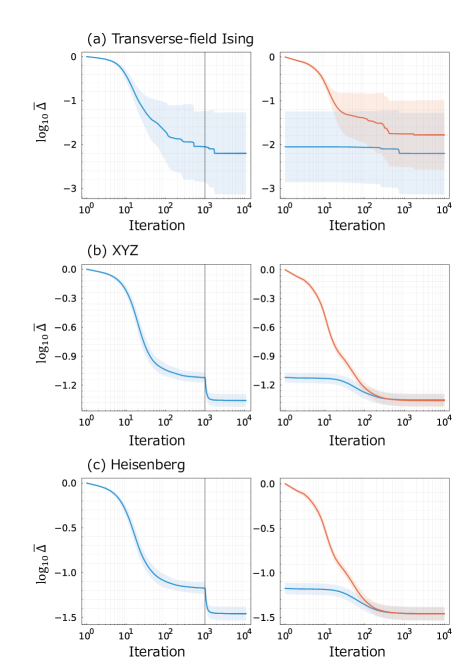
Figure 7: Iteration dependence of the random-averaged relative error $\bar{\Delta}$ in the all-to-all coupled random (a) transverse-field Ising, (b) XYZ, and (c) Heisenberg model (left panels), and comparison of $\bar{\Delta}$ in the VQE calculation using initial states with embedded MERA states after TN optimizations and random branching MERA states (right panels).

In all three models, the optimization of the MERA state is almost completed up to $10^{3}$ iterations; in fact, we confirm that this claim is true by increasing the number of iterations up to $5\times 10^{3}$. After the quantum circuit encoding of the MERA state, we perform the VQE calculation, and the $\log_{10}\bar{\Delta}$ decreases by 0.15, 0.23, and 0.28 in the all-to-all coupled random Ising model, XYZ model, and Heisenberg model reflecting the entanglement augmentations. In particular, for the XYZ and Heisenberg models since they have more quantum fluctuation so the intensity of off-diagonal components may be comparable with it’s of diagonal components, the accuracy improvements by the entanglement augmentation are greater than for the Ising model.

The right panel of Fig. 7 focuses on the VQE calculation part and compares the behaviors of $\bar{\Delta}$ with two initial conditions: optimized MERA states and random branching MERA states. In the case of the all-to-all coupled random transverse-field Ising model, there is a moderately large initial-state dependence on the converged $\bar{\Delta}$, and the VQE with random branching MERA as the initial state is clearly trapped local minima. This is a specific example where the EEVQE results show an advantage over the standard VQE. On the other hand, in the case of the all-to-all coupled random XYZ and Heisenberg model, there is no significant difference about converged $\bar{\Delta}$ for both initial conditions. However, up to about $10^{2}$ iterations of VQE, EEVQE can reduce $\bar{\Delta}$ compared to VQE where the random branching MERA states are initial states. This result suggests that the short-time VQE computation using the NISQ device is superior in our procedure, consistent with the current trend of quantum algorithm development.

V Conclusion and Discussion

We have developed an entangled embedded VQE (EEVQE) method that uses a branching binary MERA with a one-dimensional entropic volume law as the ansatz for VQE calculations. In the EEVQE method, the binary MERA is optimized using a modified Evenbly-Vidal method on a classical computer and serves as the initial state for VQE. Unlike the original synergistic frameworks[10] that use TN structure only for the initial state, EEVQE incorporates an entanglement augmentation topology based on TN structure during gate addition. We investigated the performance of our method on the all-to-all coupled random transverse field Ising model, XYZ model, and Heisenberg model, evaluating the random average $\bar{\Delta}$ of the relative error between the variational energy and the exact ground state energy under computational condition $(\chi,N)=(2,16)$ for obtaining the exact quantum circuit representation of the branching MERA embedded with the optimized MERA and the exact ground state of each model.

In the numerical simulation, first, we examined the benchmark of MERA optimization procedure on the classical computer about three methods, the Evenbly-Vidal algorithm, its modification, and the BFGS method as a fundamental knowledge of MERA for non-uniform systems. The results show that the BFGS method is superior to other methods for every model we studied. This trend is considered to be a phenomenon specific to non-uniform systems since similar analysis in uniform systems [16] shows that sequential local updating by the Evenbly-Vidal method is superior to the gradient-based methods. This property becomes crucial when using the synergistic framework to study the ground states of quantum chemical calculations, which is the one of goals of VQE for all-to-all coupled inhomogeneous systems.

Second, we verified the EEVQE method reduces $\log_{10}\bar{\Delta}$ by 0.15, 0.23, 0.28 in the all-to-all coupled random Ising, XYZ, and Heisenberg, reflecting the entanglement augmentations while free from the initialization problem of VQE calculations. Furthermore, in the all-to-all coupled random Ising model, we confirm that EEVQE can prevent getting stuck in a local minimum, while the VQE with randomly-initialized branching-MERA ansatz may get trapped in the minimum. Also, a comparison of VQE with random initialized branching MERA and branching MERA with embedded an optimized binary MERA as the initial state shows that the latter is superior to the former up to about $10^{2}$ iterations of the update in VQE. These properties meet the requirements of the quantum variational algorithm using the NISQ device, which is to improve the accuracy of the best solution on a classical computer by a small amount of use of a quantum computer.

In the present study, since we applied one-dimensional branching MERA ansatz to a non-uniform system with all-to-all coupled interactions, obtaining a highly accurate $\bar{\Delta}$ was not easy with $\chi=2$, even for the TN that satisfies the entropic volume law. If we can perform structural optimization of TN for each realization of random interaction, $\bar{\Delta}$ with higher accuracy is expected to be easily obtained even for TN with the current minimum degree of freedom, $\chi=2$. There have been reports on the structure optimization for TTNs that do not include loop structures in the TN [53, 54, 55]. However, these optimizations naively cannot be applied straightforwardly to MERA, including loop structures, and future research is needed.

As another future research, it is also important to consider a scheme to handle a more general bond dimension $\chi$. In this case, it is possible to apply automatic quantum circuit encoding (AQCE) [41] or other circuit decomposition tequniques [34, 35, 36, 37, 38, 39, 40, 41, 42, 43, 44, 45] to each disentangler, isometry, and top tensor of the TN to perform divide-and-conquer quantum circuit encoding for the entire TN.

Also, a deep MERA (DMERA) [56] has been reported as an algorithm that mixes the roles between the disentangler and isometry in MERA and improves the performance of MERA through quantum circuit representation. We can also introduce the branching degree of freedom in the DMERA. By looking at the TN microscopically in terms of the product of two-qubit gates, it will be more necessary to design a TN/quantum circuit structure that matches the geometrical aspect of the entanglement that the target state contains.

Other methods not treated in this study as optimizers for updating MERA include learning rate [30], automatic differentiation [57], and Riemannian optimization [27], and it is interesting to verify whether these methods perform better than the BFGS method in the all-to-all coupled non-uniform models as one of the future issues to be addressed.

Finally, of course, we should address the verification of EEVQE on actual NISQ devices as a future study.

Appendix A Unitarization of isometry by Modified Gram-Schmidt method

We consider the isometry $w=\{w^{c}_{ab}\}_{1\leq a,b\leq\chi}^{1\leq c\leq\chi^{\prime}}$ , where $\chi^{\prime}$ meets $1\leq\chi^{\prime}\leq\chi^{2}$, with a given bond dimension $\chi,\chi^{\prime}$ of a positive integer has the isometric condition in Eq. (3). For unitarization of the isometry $w$, we introduce a four-rank tensor $u=\{u^{cd}_{ab}\}_{1\leq a,b\leq\chi}^{1\leq c\leq\chi^{\prime},1\leq d\leq\chi^{2}/\chi^{\prime}}$ and embed $w$ and a random tensor $r=\{r^{cm}_{ab}\}_{1\leq a,b\leq\chi}^{1\leq c\leq\chi^{\prime},2\leq m\leq\chi^{2}/\chi^{\prime}}$ into $u$ as

$$u^{cd}_{ab}=\left\{\begin{matrix}w^{c}_{ab}&(d=1)\\ r^{cd}_{ab}&(2\leq d\leq\chi^{2}/\chi^{\prime})\\ \end{matrix}\right.~{}.$$ (20)

Then, we perform the modified Gram-Schmidt procedures in Algorithm 1 and obtain the isometric tensor $u$ that satisfies the isometric conditions in Eq. (1) and Eq. (2).

Algorithm 1 the modified Gram-Schmidt procedures

1:  for $c=1:\chi^{\prime}$, $d=2:\chi^{2}/\chi^{\prime}$ do

2:     for $n=1:c+\chi^{\prime}(d-1)-1$ do

3:        find $c^{\prime}$ and $d^{\prime}$ that satisfy $n=c^{\prime}+\chi^{\prime}(d^{\prime}-1)$

4:        $u_{:,:}^{cd}:=u_{:,:}^{cd}-\left(\sum_{a,b}u_{ab}^{c^{\prime}d^{\prime}*}u_{ab}^{cd}\right)u_{:,:}^{c^{\prime}d^{\prime}}$

5:        (Note that $u_{:,:}^{cd}=\{u_{ab}^{cd}\}_{1\leq a,b\leq\chi}$.)

6:     end for

7:     $u_{:,:}^{cd}:=u_{:,:}^{cd}/||u_{:,:}^{cd}||_{2}$

8:  end for

Appendix B Network dependence of the performance of modified Evenbly-Vidal method

In Fig. 8, we conducted a study on the performance of the modified Evenbly-Vidal method for inhomogeneous MERAs with all branching patterns, as shown in Fig. 2. Our results indicate that, in all model and branching pattern combinations, the modified method outperforms the original Evenbly-Vidal method during the initial optimization iterations up to $10^{2}$. Additionally, this improvement is more significant in both models as the number of top tensors increases due to bifurcations.

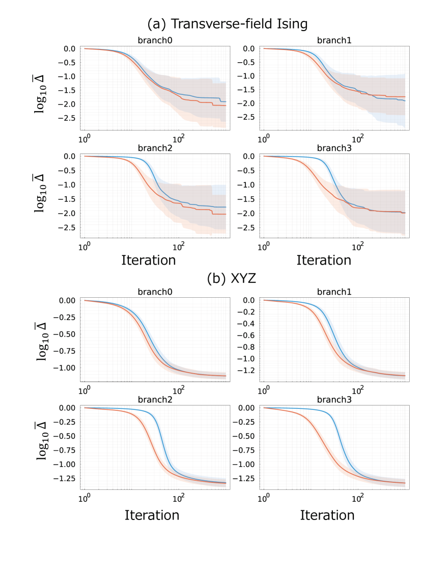
Figure 8: Iteration dependence of $\bar{\Delta}$ for all-to-all coupled random (a) Ising and (b) XYZ systems with $(\chi,N)=(2,16)$. The blue and orange lines represent the case of the Evenbly-Vidal method and its modification, as we introduced in Sec. III.2, respectively. The branching pattern was named according to the manner in Fig. 2.

References

- Daskin and Kais [2018] A. Daskin and S. Kais, Chem. Phys. 514, 87 (2018).
- Low and Chuang [2019] G. H. Low and I. L. Chuang, Quantum 3, 163 (2019).
- Gilyén et al. [2019] A. Gilyén, Y. Su, G. H. Low, and N. Wiebe, in Proceedings of the 51st Annual ACM SIGACT Symposium on Theory of Computing (ACM, 2019) p. 193â204.
- Preskill [2018] J. Preskill, Quantum 2, 79 (2018).
- Cerezo et al. [2021] M. Cerezo, A. Arrasmith, R. Babbush, S. C. Benjamin, S. Endo, K. Fujii, J. R. McClean, K. Mitarai, X. Yuan, L. Cincio, and P. J. Coles, Nat. Rev. Phys. 3, 625 (2021).
- Peruzzo et al. [2014] A. Peruzzo, J. McClean, P. Shadbolt, M.-H. Yung, X.-Q. Zhou, P. J. Love, A. Aspuru-Guzik, and J. L. O’Brien, Nat. Commun. 5, 4213 (2014).
- McClean et al. [2018] J. R. McClean, S. Boixo, V. N. Smelyanskiy, R. Babbush, and H. Neven, Nat. Commun. 9, 4812 (2018).
- Grant et al. [2019] E. Grant, L. Wossnig, M. Ostaszewski, and M. Benedetti, Quantum 3, 214 (2019).
- Okada et al. [2022] K. N. Okada, K. Osaki, K. Mitarai, and K. Fujii, (2022), arXiv:2202.02909 [quant-ph] .
- Rudolph et al. [2022a] M. S. Rudolph, J. Miller, J. Chen, A. Acharya, and A. Perdomo-Ortiz, (2022a), arXiv:2208.13673 [quant-ph] .
- Orús [2014] R. Orús, Ann. Phys. 349, 117 (2014).
- Orús [2014] R. Orús, Eur. Phys. J. B 87, 280 (2014).
- Ran et al. [2020] S.-J. Ran, E. Tirrito, C. Peng, X. Chen, L. Tagliacozzo, G. Su, and M. Lewenstein, Tensor network contractions: methods and applications to quantum many-body systems (Springer Nature, 2020).
- Okunishi et al. [2022] K. Okunishi, T. Nishino, and H. Ueda, J. Phys. Soc. Jpn. 91, 062001 (2022).
- Liu et al. [2019] J.-G. Liu, Y.-H. Zhang, Y. Wan, and L. Wang, Phys. Rev. Res. 1, 023025 (2019).
- Haghshenas et al. [2022] R. Haghshenas, J. Gray, A. C. Potter, and G. K.-L. Chan, Phys. Rev. X 12, 011047 (2022).
- Miao and Barthel [2023] Q. Miao and T. Barthel, (2023), arXiv:2303.08910 [quant-ph] .
- White [1992] S. R. White, Phys. Rev. Lett. 69, 2863 (1992).
- Schollwöck [2011] U. Schollwöck, Ann. Phys. 326, 96 (2011), january 2011 Special Issue.
- Zauner-Stauber et al. [2018] V. Zauner-Stauber, L. Vanderstraeten, M. T. Fishman, F. Verstraete, and J. Haegeman, Phys. Rev. B 97, 045145 (2018).
- Eisert et al. [2010] J. Eisert, M. Cramer, and M. B. Plenio, Rev. Mod. Phys. 82, 277 (2010).
- Goldsborough and Evenbly [2017] A. M. Goldsborough and G. Evenbly, Phys. Rev. B 96, 155136 (2017).
- Vidal [2008] G. Vidal, Phys. Rev. Lett. 101, 110501 (2008).
- Evenbly and Vidal [2009] G. Evenbly and G. Vidal, Phys. Rev. B 79, 144108 (2009).
- Evenbly and Vidal [2014a] G. Evenbly and G. Vidal, Phys. Rev. Lett. 112, 240502 (2014a).
- Evenbly and Vidal [2014b] G. Evenbly and G. Vidal, Phys. Rev. B 89, 235113 (2014b).
- Hauru et al. [2021] M. Hauru, M. V. Damme, and J. Haegeman, SciPost Phys. 10, 040 (2021).
- Mitarai et al. [2018] K. Mitarai, M. Negoro, M. Kitagawa, and K. Fujii, Phys. Rev. A 98, 032309 (2018).
- Tilly et al. [2022] J. Tilly, H. Chen, S. Cao, D. Picozzi, K. Setia, Y. Li, E. Grant, L. Wossnig, I. Rungger, G. H. Booth, and J. Tennyson, Phys. Rep. 986, 1 (2022).
- Rudolph et al. [2022b] M. S. Rudolph, J. Chen, J. Miller, A. Acharya, and A. Perdomo-Ortiz, (2022b), arXiv:2209.00595 [quant-ph] .
- Ran [2020] S.-J. Ran, Phys. Rev. A 101, 032310 (2020).
- Tucci [2005] R. R. Tucci, (2005), arXiv:quant-ph/0507171 [quant-ph] .
- Kraus and Cirac [2001] B. Kraus and J. I. Cirac, Phys. Rev. A 63, 062309 (2001).
- DiVincenzo and Smolin [1994] D. DiVincenzo and J. Smolin, in Proceedings Workshop on Physics and Computation. PhysComp ’94 (1994) pp. 14–23.
- Amy et al. [2013] M. Amy, D. Maslov, M. Mosca, and M. Roetteler, IEEE T. Comput. Aid. D. 32, 818 (2013).
- Nam et al. [2018] Y. Nam, N. J. Ross, Y. Su, A. M. Childs, and D. Maslov, Npj Quantum Inf. 4, 23 (2018).
- Khatri et al. [2019] S. Khatri, R. LaRose, A. Poremba, L. Cincio, A. T. Sornborger, and P. J. Coles, Quantum 3, 140 (2019).
- Nagarajan et al. [2021] H. Nagarajan, O. Lockwood, and C. Coffrin, in 2021 IEEE/ACM Second International Workshop on Quantum Computing Software (QCS) (2021) pp. 55–63.
- Younis et al. [2021] E. Younis, K. Sen, K. Yelick, and C. Iancu, (2021), arXiv:2103.07093 [quant-ph] .
- Fösel et al. [2021] T. Fösel, M. Y. Niu, F. Marquardt, and L. Li, (2021), arXiv:2103.07585 [quant-ph] .
- Shirakawa et al. [2021] T. Shirakawa, H. Ueda, and S. Yunoki, (2021), arXiv:2112.14524 [quant-ph] .
- Meister et al. [2022] R. Meister, C. Gustiani, and S. C. Benjamin, (2022), arXiv:2206.11245 [quant-ph] .
- Rakyta and Zimborás [2022] P. Rakyta and Z. Zimborás, (2022), arXiv:2203.04426 [quant-ph] .
- Nemkov et al. [2023] N. A. Nemkov, E. O. Kiktenko, I. A. Luchnikov, and A. K. Fedorov, (2023), arXiv:2205.01121 [quant-ph] .
- Smith et al. [2023] E. Smith, M. G. Davis, J. Larson, E. Younis, L. B. Oftelie, W. Lavrijsen, and C. Iancu, ACM Trans. Quantum Comput. 4, 5 (2023).
- Shi et al. [2006] Y.-Y. Shi, L.-M. Duan, and G. Vidal, Phys. Rev. A 74, 022320 (2006).
- Tagliacozzo et al. [2009] L. Tagliacozzo, G. Evenbly, and G. Vidal, Phys. Rev. B 80, 235127 (2009).
- Murg et al. [2010] V. Murg, F. Verstraete, O. Legeza, and R. M. Noack, Phys. Rev. B 82, 205105 (2010).
- Fishman et al. [2022] M. Fishman, S. R. White, and E. M. Stoudenmire, SciPost Phys. Codebases , 4 (2022).
- Developers [2022] C. Developers, Cirq (2022).
- Suzuki et al. [2021] Y. Suzuki, Y. Kawase, Y. Masumura, Y. Hiraga, M. Nakadai, J. Chen, K. M. Nakanishi, K. Mitarai, R. Imai, S. Tamiya, T. Yamamoto, T. Yan, T. Kawakubo, Y. O. Nakagawa, Y. Ibe, Y. Zhang, H. Yamashita, H. Yoshimura, A. Hayashi, and K. Fujii, Quantum 5, 559 (2021).
- Virtanen et al. [2020] P. Virtanen, R. Gommers, T. E. Oliphant, M. Haberland, T. Reddy, D. Cournapeau, E. Burovski, P. Peterson, W. Weckesser, J. Bright, S. J. van der Walt, M. Brett, J. Wilson, K. J. Millman, N. Mayorov, A. R. J. Nelson, E. Jones, R. Kern, E. Larson, C. J. Carey, İ. Polat, Y. Feng, E. W. Moore, J. VanderPlas, D. Laxalde, J. Perktold, R. Cimrman, I. Henriksen, E. A. Quintero, C. R. Harris, A. M. Archibald, A. H. Ribeiro, F. Pedregosa, P. van Mulbregt, and SciPy 1.0 Contributors, Nat. Methods 17, 261 (2020).
- Li et al. [2022] W. Li, J. Ren, H. Yang, and Z. Shuai, J. Phys. Condens. Matter 34, 254003 (2022).
- Hikihara et al. [2023] T. Hikihara, H. Ueda, K. Okunishi, K. Harada, and T. Nishino, Phys. Rev. Res. 5, 013031 (2023).
- Okunishi et al. [2023] K. Okunishi, H. Ueda, and T. Nishino, Prog. Theor. Exp. Phys. 2023, 023A02 (2023).
- Kim and Swingle [2017] I. H. Kim and B. Swingle, (2017), arXiv:1711.07500 [quant-ph] .
- Geng et al. [2022] C. Geng, H.-Y. Hu, and Y. Zou, Mach. learn.: sci. technol. 3, 015020 (2022).