Decoherence Time Induced by The Noise of Primordial Graviton With Minimum Uncertainty Initial States

Abstract

We have investigated the decoherence time induced by the primordial gravitons with minimum uncertainty initial states. This minimum uncertainty condition allows the initial state to be an entanglement or, more generally, a superposition between a vacuum and an entanglement state. We got that for initial state entanglement, the decoherence time will last a maximum of 20 seconds, similar to the initial Bunch-Davies vacuum, and if the total graviton is greater than zero, the dimensions of the experimental setup system could be reduced. We also found that quantum noise can last much longer than vacuum or entanglement states for initial state superposition, which will be maintained for $\approx 10^{19}$ seconds.

Keywords— Minimum Uncertainty, Primordial Graviton and Decoherence

1 Introduction

One prediction from Einstein’s general theory of relativity is the phenomenon of gravitational waves [1, 2]. When there is a compact concentration of energy, spacetime will bend. If the concentration of energy changes, it will produce dynamics in the curvature of spacetime that will propagate in all directions at the speed of light. The propagation of the dynamic curvature of spacetime in all directions is what we know as gravitational waves. In the last decades, gravitational waves have been attempted to be detected. Until 2015, the LIGO detector succeeded in detecting gravitational waves for the first time [3]. This success has become a hope for detecting another phenomenon related to gravitational waves in the future. One of those phenomena is looking for the quantum characteristics of gravitational waves as graviton particles. This phenomenon is interesting because graviton particles are one of the consequences that arise from the quantization of gravity. As we know, there has been no satisfactory theory for the quantum theory of gravity up until now. Some scientists even believe that gravity has not to be quantized at all [4]. Even so, many scientists are still trying to develop a mechanism to detect gravitons.

Several studies related to graviton detection are still being developed today [5, 6, 7, 8, 9, 10, 11, 12, 13, 14]. The interesting one is the research proposed by Parikh et. al. [5]. They submitted a study proposal to detect graviton through the quantum noise effect produced by these particles on classical masses with the same vein as quantum Brownian motion [15, 16]. The idea of this detection is based on the assumption that detecting individual gravitons is impossible [17]. In his research, Parikh et. al. [5] studied the behavior of a gravitational wave detector in response to a quantized gravitational field. The detector will be modeled as two objects that are geodesically separated. Then, using the Feynman-Vernon influence functional method [18, 19], the quantum noise generated from the quantized gravitational field can be studied. Furthermore, this study was expanded by S. Kanno et. al. [8], where they study the decoherence time between the detector and the environment with a quantized gravitational field to determine how long quantum noise could be detected. Another research was conducted by H. T. Cho and B. L. Hu [14], where the study was expanded by considering all possible graviton modes, including polarization. These studies show similar results where quantum noise can be detected if the initial quantum state is squeezed.

Gravitational waves could originate from several places, for example, black holes [20, 21, 22], neutron stars [23, 24], or from the early universe when the inflation mechanism occurred [25, 26, 27]. The gravitational wave from the early universe is called a primordial gravitational wave. Some of the best cosmological inflation models that can explain the structure of our universe with great precision predict that the universe started from a quantum state [28, 29, 30, 31, 32, 33]. This means that the primordial gravitational waves also originate from the quantum state. So, gravitons would have been generated in the early universe. Interestingly, due to inflation at the beginning of the universe, the initial quantum state was believed to be squeezed as the universe expanded [34]. This means that if gravitons came from the early universe, it should be possible to detect gravitons using the quantum noise method. The proposal to detect primordial gravitons was put forward by S. Kanno et al. [9]. In their proposal, they proposed an experimental setup that could be used to detect noise generated from primordial gravitons. The result shows that the quantum noise of gravitons from the early universe can be detected in 20 seconds. However, the quantum initial state of the graviton used is only the Bunch-Davies vacuum. In quantum field theory, a vacuum state is an essential quantum state with the lowest possible energy and generally does not contain physical particles. Although the initial state is usually chosen to be a vacuum, it does not rule out the possibility that it could take the form of another state. In this research, we want to expand the understanding of this study by assuming the initial state is a state other than a vacuum. By studying decoherence time from different forms of the initial state, we hope to obtain the possibility of a more extended time for detecting noise produced by primordial gravitons.

One of the basic concepts that differentiates classical from quantum physics is the Heisenberg uncertainty principle, which is a concept that limits the measurement accuracy of two observables in a system. This limitation exists not because of the inability of the measuring instrument but because of nature itself. The highest measurement accuracy (the condition where measurement accuracy in quantum mechanics is closest to the classical concept) can occur if the quantum state is a solution of the minimum uncertainty relation [35], called the minimum uncertainty state. Because there was a transition from the quantum to the classical states in the early universe, it does not rule out the possibility that the initial state was a state with measurement accuracy closest to classical physics, namely, a state of minimal uncertainty. Observables that can be analyzed from gravitational waves are needed to obtain an initial state of minimum uncertainty of primordial gravitons. In this research, the observable that will be used is observables that describe the polarization intensity of gravitational waves with measurement operators that can be represented in the form of the Stoke operator [36]. There are four Stokes operators, each of which will define the intensity of linear, circular, and total polarization of the gravitons. By using these operators, the minimum uncertainty state should be a unique quantum state (for example, entanglement state as in the research [37, 38, 39, 40]). This unique quantum state should be able to increase the quantumness of primordial gravitational waves so that the decoherence time induced by the noise of primordial gravitons can last longer than 20 seconds.

The organization of this paper is as follows. First, in section 2, we will explain the possible initial states of minimum uncertainty based on Stoke operators. Then, in section 3, we will review quantum noise operators caused by graviton particles, such as the research from S. Kanno et al.. [8]. In section 4, we will calculate the decoherence time caused by noise from primordial gravitons with initial states in the form of minimum uncertainty obtained in section 2 using the same experimental setup as the research from S. Kanno et al.. [9]. The last section is the conclusion. This paper will include Appendix, which contains the influence functional method used to determine the decoherence functional due to the noise of graviton, which will be used in the section 4 to calculate the decoherence time.

2 Minimum Uncertainty of Graviton

In quantum mechanics, if there are two hermitian operators $\hat{X}_{1}$ and $\hat{X}_{2}$, the Heisenberg uncertainty relation can be expressed as $\big{(}\Delta\hat{X}_{1}\big{)}^{2}\big{(}\Delta\hat{X}_{2}\big{)}^{2}\geq\frac{1}{4}|\braket{\big{[}\hat{X}_{1},\hat{X}_{2}\big{]}}|^{2}$. A quantum state can be said to fulfil its minimal conditions or minimal uncertainty if the quantum state is a solution to the eigenequation [35]

$$\big{(}\hat{X}_{1}+i\lambda\hat{X}_{2}\big{)}\ket{\psi}=\beta\ket{\psi},$$ (2.1)

where $\beta$ is the eigenvalue and $\lambda$ is the squeezing parameter of the solution of the eigenstate. The squeezed parameter $\lambda$ will determine the initial quantum state of the system in its minimal uncertainty condition. To see why $\lambda$ is defined as the squeezing parameter, it can be explained by looking for the variance of the $\hat{X}_{1}$ and $\hat{X}_{2}$ operators based on the minimal uncertainty relation (2.1). The variance can be written as follows

$$\big{(}\Delta\hat{X}_{1}\big{)}^{2}=\frac{1}{2}\lambda\,\,\,|\bra{\psi}[\hat{X}_{1},\hat{X}_{2}]\ket{\psi}|$$ (2.2)

and

$$(\Delta\hat{X}_{2})^{2}=\frac{1}{2\lambda}\,\,\,\big{|}\bra{\psi}[\hat{X}_{1},\hat{X}_{2}]\ket{\psi}\big{|}.$$ (2.3)

It can be seen that when $\lambda<1$, the variance of equation (2.3) will be greater than equation (2.2). Based on the definition of a squeezed state [45, 46], a quantum state can be said to be squeezed if the variance of one operator that satisfies the minimum uncertainty is smaller than the variance of the other operators, which means that when $\lambda<1$ the quantum state will be squeezed. It also applies when $\lambda>1$ except that the variance of equation (2.2) will be larger than equation (2.3). When $\lambda=0$, the stated will not be squeezed because the two variances are the same. Furthermore, for simplicity of calculation, the value of $\lambda$ will be limited to $0\leq\lambda\leq 1$.

To find out the minimum uncertainty relation of the primordial graviton, the arbitrary operators $\hat{X}_{1}$ and $\hat{X}_{2}$ in equation (2.1) are chosen to be operators that define the polarization of gravitational waves. Like the photon, the polarization of gravitational waves can be defined by the Stokes operators. Using the representation of annihilation and creation operators of graviton, the Stokes operator can be expressed as

$$\hat{\mathcal{S}}^{(0)}_{k} = \hat{a}^{\oplus\dagger}_{\mathbf{k}}\hat{a}^{\oplus}_{\mathbf{k}}+\hat{a}^{\otimes\dagger}_{\mathbf{k}}\hat{a}^{\otimes}_{\mathbf{k}},\,\,\,\,\,\,\,\hat{\mathcal{S}}^{(1)}_{k}=\hat{a}^{\oplus\dagger}_{\mathbf{k}}\hat{a}^{\oplus}_{\mathbf{k}}-\hat{a}^{\otimes\dagger}_{\mathbf{k}}\hat{a}^{\otimes}_{\mathbf{k}}$$

$$\hat{\mathcal{S}}^{(2)}_{k} = \hat{a}^{\oplus\dagger}_{\mathbf{k}}\hat{a}^{\otimes}_{\mathbf{k}}+\hat{a}^{\oplus}_{\mathbf{k}}\hat{a}^{\otimes\dagger}_{\mathbf{k}},\,\,\,\,\,\,\,\hat{\mathcal{S}}^{(3)}_{k}=i\big{(}\hat{a}^{\oplus}_{\mathbf{k}}\hat{a}^{\otimes\dagger}_{\mathbf{k}}-\hat{a}^{\oplus\dagger}_{\mathbf{k}}\hat{a}^{\otimes}_{\mathbf{k}}\big{)}.$$ (2.4)

The operator $\mathcal{S}^{(0)}_{k}$ defines the total intensity of all modes of the gravitons. $\mathcal{S}^{(1)}_{k}$ and $\mathcal{S}^{(2)}_{k}$ are intensity operators of linear polarization. Meanwhile, $\mathcal{S}^{(3)}_{k}$ is an operator for measuring the intensity of circular polarization. The last three Stokes operators will have a commutation relation $[\hat{\mathcal{S}}^{(i)}_{k},\hat{\mathcal{S}}^{(j)}_{k}]=2i\epsilon^{ijk}\hat{\mathcal{S}}^{(k)}_{k}$ which satisfies the SU(2) algebra with $(i,j,k)\equiv 1,2,3$. However, for operator $\mathcal{S}^{(0)}_{k}$, the commutation relations with other operators will always be zero, which means the operator $\mathcal{S}^{(0)}_{k}$ cannot be used to study minimal uncertainty.

Furthermore, by choosing arbitrary operators $\hat{X}_{1}$ and $\hat{X}_{2}$ as the stoke operators, then the minimum uncertainty states of the primordial graviton, which will be used as initial states of the early universe, can be obtained. First we chose the arbitrary operators $\hat{X}_{1}=\hat{S}^{(2)}_{k}$ and $\hat{X}_{2}=\hat{S}^{(3)}_{k}$ . Substitute into equation (2.1), the minimum uncertainty relation will be obtained as

$$\bigg{[}(1+\lambda)\hat{a}^{\oplus\dagger}_{\mathbf{k}}\hat{a}^{\otimes}_{\mathbf{k}}+(1-\lambda)\hat{a}^{\oplus}_{\mathbf{k}}\hat{a}^{\otimes\dagger}_{\mathbf{k}}\bigg{]}\ket{\psi}=\beta\ket{\psi}.$$ (2.5)

As explained in the first pharagraph, there are three possible values of $\lambda$ which are $\lambda=0$, $\lambda=1$ and $0<\lambda<1$. For $\lambda=0$ the minimum uncertainty relation become

$$\bigg{[}\hat{a}^{\oplus\dagger}_{\mathbf{k}}\hat{a}^{\otimes}_{\mathbf{k}}+\hat{a}^{\oplus}_{\mathbf{k}}\hat{a}^{\otimes\dagger}_{\mathbf{k}}\bigg{]}\ket{\psi}=\beta\ket{\psi}.$$ (2.6)

To obtain the solution, the general form of the quantum state is taken $\ket{\psi}=\sum_{n,m}\mathcal{C}_{nm}\ket{n^{\oplus}_{\mathbf{k}},m^{\otimes}_{\mathbf{k}}}$. Where $\mathcal{C}_{nm}$ is a constant that depends on the value of $n$ and $m$. Substitute back into equation (2.6), then multiply by $\bra{i^{\oplus}_{\mathbf{k}},j^{\otimes}_{\mathbf{k}}}$ from the left, we got

$$\sqrt{i(j+1)}\mathcal{C}_{(i-1)\,(j+1)}+\sqrt{(i+1)(j-1)}\,\,\mathcal{C}_{(i+1)\,(j-1)}=\beta\,\,\mathcal{C}_{ij}.$$ (2.7)

The constant $\beta$ is chosen to be the total number of gravitons $(N=n+m)$, then the constant $\mathcal{C}_{nm}$ can be found to be $\begin{pmatrix}N\\ n\end{pmatrix}^{1/2}$. So, the solution to the eigenstate become

$$\ket{\psi} = \sum_{n=0}^{N}\,\,\frac{1}{2^{N/2}}\,\,\begin{pmatrix}N\\ n\end{pmatrix}^{1/2}\ket{(N-n)^{\oplus}_{\mathbf{k}},\,\,n^{\otimes}_{\mathbf{k}}}.$$ (2.8)

where $1/2^{N/2}$ appears due to normalization. This state is an entanglement between the polarization of modes $\oplus$ and $\otimes$. As explained in the introduction, the state of minimal uncertainty from the polarization of gravitational waves can be a state of entanglement. It is known well that the entanglement state is a unique condition in quantum physics that does not exist in classical physics. This means that if the initial state is a state of minimal uncertainty with a solution like the equation (2.8), then it should increase the quantumness level of primordial gravitational waves rather than the vacuum state. So, this initial state should be able to bring an improvement in an attempt at the detection of the primordial graviton.

For $\lambda=1$, the equation (2.5) becomes $2\hat{a}^{\oplus\dagger}_{\mathbf{k}}\hat{a}^{\otimes}_{\mathbf{k}}\ket{\psi}=\beta\ket{\psi}$. There will be a solution if $\beta=0$ with the eigenstate being a vacuum for the polarization of mode $\otimes$ and can be any state for the mode $\oplus$ ($\ket{\psi}=\ket{\phi^{\oplus},\,0^{\otimes}}$ or for simplicity is chosen $\ket{\psi}=\ket{0^{\oplus},0^{\otimes}}$). Likewise if the $\lambda$ constant is $0<\lambda<1$, the solution will also only be a vacuum state ($\ket{\psi}=\ket{0^{\oplus},0^{\otimes}}$) with $\beta=0$. So, the vacuum state will be the solution for $0\leq\lambda<1$.

To obtain a general solution of the equation (2.5), each solution for each value of $\lambda$ will be expressed in the form of a linear combination or superposition. In this case, there are only two solutions, which are a vacuum state and the entanglement (2.8). So the general solution of the minimum uncertainty relation (2.5) will be a superposition between a vacuum state and entanglement (2.8), where mathematically, it can be written as follows

$$\ket{\psi}=f_{1}(\lambda)\,\,\ket{0^{\oplus},0^{\otimes}}+f_{2}(\lambda)\sum_{n=0}^{N}\,\,\frac{1}{2^{N/2}}\,\,\begin{pmatrix}N\\ n\end{pmatrix}^{1/2}\ket{(N-n)^{\oplus}_{\mathbf{k}},\,\,n^{\otimes}_{\mathbf{k}}},$$ (2.9)

with $f_{1}(\lambda)$ and $f_{2}(\lambda)$ are functions that depend on $\lambda$. Because the equation (2.9) must be normalized $(\braket{\psi}{\psi}=1)$, then the two functions will satisfy the relation $|f_{1}(\lambda)|^{2}+|f_{2}(\lambda)|^{2}=1$. Based on this, it is chosen

$$f_{2}(\lambda)=\Big{(}1-|f_{1}(\lambda)|\Big{)}^{1/2}.$$ (2.10)

When $\lambda=1$ the equation (2.9) have to be the equation (2.8), it means the function $f_{1}(\lambda)=0$ and $f_{2}(\lambda)=1$. On the other hand, when $0\leq\lambda<1$, the equation (2.9) must be a vacuum state, meaning that $f_{1}(\lambda)=1$ and $f_{2}(\lambda)=0$. So, it can be said that $f_{1}(\lambda)$ is a function that resembles a ladder function with the highest value being 1, and if $\lambda\simeq 1$ then $f_{1}(\lambda)\simeq 0$. For this reason, the function $f_{1}(\lambda)$ will be chosen to be a hyperbolic tangent function so that the equation (2.9) becomes

$$\ket{\psi}=\tanh u\,\,\ket{0^{\oplus},0^{\otimes}}+(1-\tanh^{2}u)^{1/2}\sum_{n=0}^{N}\,\,\frac{1}{2^{N/2}}\,\,\begin{pmatrix}N\\ n\end{pmatrix}^{1/2}\ket{(N-n)^{\oplus}_{\mathbf{k}},\,\,n^{\otimes}_{\mathbf{k}}}.$$ (2.11)

Where $u\equiv c\,\lambda$ and $c$ is an arbitrary positive real number with value $c>>1$. According to this definition, the constant $u$ has a range of values of $0\leq u<\infty$. This general solution will be a unique quantum initial state because the density matrix of this state will have non-diagonal elements. As is known, non-diagonal elements in the density matrix will only appear if the system is highly quantum. This means that this solution should also increase the quantumness of primordial gravitational waves. The solution (2.11) will also be satisfied if $\hat{X}_{1}=\hat{\mathcal{S}}^{(2)}_{k}$ and $\hat{X}_{2}=\hat{\mathcal{S}}^{(1)}_{k}$.

Not only the entanglement (2.8) but there is another entanglement state that also satisfies the minimum uncertainty relation. Selected $\hat{X}_{1}=\hat{\mathcal{S}}^{(1)}_{k}$ and $\hat{X}_{2}=\hat{\mathcal{S}}^{(3)}_{k}$, substitute to the minimum uncertainty equation (2.5), then

$$\bigg{[}\hat{a}^{\oplus\dagger}_{\mathbf{k}}\hat{a}^{\oplus}_{\mathbf{k}}-\hat{a}^{\otimes\dagger}_{\mathbf{k}}\hat{a}^{\otimes}_{\mathbf{k}}-\lambda\big{(}\hat{a}^{\oplus}_{\mathbf{k}}\hat{a}^{\otimes\dagger}_{\mathbf{k}}-\hat{a}^{\oplus\dagger}_{\mathbf{k}}\hat{a}^{\otimes}_{\mathbf{k}}\big{)}\bigg{]}\ket{\psi}=\beta\ket{\psi}.$$ (2.12)

The solution of this equation can be found using the same method as before. Chose $\lambda=1$ and using the general solution $\ket{\psi}=\sum_{n,m}\mathcal{C}_{nm}\ket{n_{\mathbf{k}}^{\oplus},m_{\mathbf{k}}^{\otimes}}$, then substituted this solution and multiplied $\bra{i^{\oplus}_{\mathbf{k}},j^{\otimes}_{\mathbf{k}}}$ from the left, we got

$$\sqrt{i(j+1)}\,\,\mathcal{C}_{(i-1)(j+1)}-\sqrt{j(i+1)}\,\,\mathcal{C}_{(i+1)(j-1)}=\Big{(}\beta-(i-j)\Big{)}\,\,\mathcal{C}_{ij},$$ (2.13)

the expression for the constant $\mathcal{C}_{nm}$ can be found if the value $\beta=0$. Where is the solution to the constant $\mathcal{C}_{nm}$ is $(-1)^{n}\begin{pmatrix}N\\ n\end{pmatrix}^{1/2}$, so

$$\ket{\psi}=\sum_{n=0}^{N}\,\,\frac{1}{2^{N/2}}\,\,(-1)^{n}\begin{pmatrix}N\\ n\end{pmatrix}^{1/2}\ket{(N-n)^{\oplus}_{\textbf{k}},\,\,n^{\otimes}_{\textbf{k}}},$$ (2.14)

with $1/2^{N/2}$ appears due to normalization. This solution is similar to the entanglement (2.8), only there is a factor $(-1)^{n}$ in the solution. For $0\leq\lambda<1$ the solution is a vacuum. So, the general solution of the equation (2.12), using the superposition expression, can be written as follows

$$\ket{\psi} = \tanh u\,\,\ket{0^{\oplus},0^{\otimes}}+(1-\tanh^{2}u)^{1/2}\sum_{n=0}^{N}\frac{1}{2^{N/2}}\,\,(-1)^{n}\,\,\begin{pmatrix}N\\ n\end{pmatrix}^{1/2}\ket{(N-n)^{\oplus}_{\textbf{k}},\,\,n^{\otimes}_{\textbf{k}}},$$ (2.15)

where the constant $u$ will be defined differently, namely $u\equiv c\,(1-\lambda)$ which has the range $0\leq u<\infty$. This solution would also be satisfied when $\hat{X}_{1}=\hat{\mathcal{S}}^{(1)}_{k}$ and $\hat{X}_{2}=\hat{\mathcal{S}}^{(3)}_{k}$.

Before studying the decoherence induced by the noise of the primordial gravitons with initial states in the form of minimal uncertainty (2.11) or (2.15), we will first review the expression of the quantum noise operator of gravitons in next section. This operator will be used to calculate the decoherence functional in section (4).

3 Quantum Noise from Graviton

This section will briefly review quantum noise caused by gravitons based on research from S. Kanno et al. [8]. Quantum noise is a consequence that arises due to an interaction between the system and the environment within the framework of quantum mechanics. His research assumes that the system is an interferometer with two mirrors in the gravitational wave environment. If the gravitational waves are quantized (in the form of graviton particles), it is expected that there will be interactions between the system and the environment. So that the quantum noise would appear when the interferometer makes the measurements. The appearance of this noise could verify the quantum characteristic of gravitational waves or the existence of the graviton particle.

The quantum noise operator can be mathematically obtained by assuming the interferometer mirror is a particle in the Fermi normal coordinates system. In this coordinates system, there are two particles, where one of those (a particle with a geodesic $\gamma_{\tau}$) will be used as a frame of reference. While the other particles (particles with geodesic $\gamma_{\tau^{\prime}}$) are test particles that have a position $x^{i}(t)=\xi^{i}(t)$ to the reference frame at point $P(0,t)$. The Fermi normal coordinates are used because of the Einstein equivalence principle, where if only one particle is considered, the effect of gravitational waves cannot be affected.

Next, consider the geodesic action of the test particles. By using the metric in Fermi coordinates for the second order of $x^{i}$ as

$$ds^{2} \simeq (-1-R_{0i0j}x^{i}x^{j})dt^{2}-\frac{4}{3}R_{0jik}x^{j}x^{k}dtdx^{i}+\Big{(}\delta_{ij}-\frac{1}{3}R_{ikjl}x^{k}x^{l}\Big{)}dx^{i}dx^{j}.$$ (3.1)

The test particle action will be obtained as

$$S_{p}\simeq\int_{\gamma_{\tau^{\prime}}}dt\Big{[}\frac{m}{2}\dot{{\xi^{i}}^{2}}-\frac{m}{2}R_{0i0j}(0,t)\xi^{i}\xi^{j}\Big{]}.$$ (3.2)

Because the mirror particle is in an environment with gravitational waves, the Riemann tensor $R_{0i0j}$ can be obtained by using a flat metric space and time with small perturbations $h_{ij}$ that satisfies the transverse traceless gauge $(\partial_{i}h^{ij}=0$, and $h^{i}_{i}=0)$. So if the perturbation $h_{ij}$ is represented in Fourier space, we get action

$$S_{p}\simeq\int_{\gamma_{\tau^{\prime}}}dt\bigg{[}\frac{m}{2}\dot{{\xi^{i}}^{2}}-\frac{m}{2}\frac{\kappa}{\sqrt{V}}\sum_{A}\sum_{\textbf{k}\leq\Omega_{m}}\ddot{h}^{A}_{\textbf{k}}(t)\,\,e^{A}_{\textbf{k},ij}\,\,\xi^{i}\xi^{j}\bigg{]},$$ (3.3)

where $\sum_{\textbf{k}\leq\Omega_{m}}$ represents the sum of k modes, with UV cutoof $\Omega_{m}\sim\xi^{-1}$. In general, the total action can be written as the sum of the actions of the test particles plus the gravitational action $(S=S_{p}+S_{g})$, which can be written as follows

$$S \simeq \int dt\sum_{\textbf{k},A}\bigg{[}\frac{1}{2}\dot{h}^{A}_{\textbf{k}}(t)\dot{h}^{*A}_{\textbf{k}}(t)-\frac{1}{2}k^{2}h^{A}_{\textbf{k}}(t)h^{*A}_{\textbf{k}}(t)\bigg{]}+\int dt\bigg{[}\frac{m}{2}\dot{{\xi^{i}}^{2}}-\frac{m}{2}\frac{\kappa}{\sqrt{V}}\sum_{A}\sum_{\textbf{k}\leq\Omega_{m}}\ddot{h}^{A}_{\textbf{k}}(t)\,\,e^{A}_{\textbf{k},ij}\,\,\xi^{i}\xi^{j}\bigg{]}.$$

The gravitational action in the first term is just an action with the equation of motion similar to a harmonic oscillator. By using the interaction picture, the field $h^{A}_{I,\textbf{k}}(t)$ can be quantized by defining it in terms of the annihilation and creation operators

$$\hat{h}^{A}_{\textbf{k},I}(t)=\hat{a}^{A}_{\textbf{k}}v_{k}(t)+\hat{a}^{A\dagger}_{-\textbf{k}}v^{*}_{k}(t)$$ (3.5)

Where $v_{k}(t)$ is the solution to the equation of motion which has the form $v_{k}(t)=(1/\sqrt{2k})e^{-ikt}$ and the annihilation and creation operators would satisfy $[\hat{a}^{A}_{\textbf{k}}\hat{a}^{A^{\prime}\dagger}_{\textbf{k}^{\prime}}]=\delta_{A,A^{\prime}}\delta_{\textbf{k}\textbf{k}^{\prime}}$. Next, the field $\hat{h}^{A}_{I,\textbf{k}}(t)$ will be divided into two parts, namely the ”classic” part $\Big{(}h_{cl,\textbf{k}}(t)\equiv\braket{\hat{h}^{A}_{\textbf{k},I}(t)}\Big{)}$ and the ”quantum” part which can be written as

$$\delta\hat{h}^{A}_{\textbf{k},I}(t)=\hat{h}^{A}_{\textbf{k},I}(t)-h_{cl,\textbf{k}}(t).$$ (3.6)

From this equation, one could say that $\delta\hat{h}^{A}_{I,\textbf{k}}(t)$ will define the quantum fluctuations of gravitational waves due to graviton particles. To review the expression of the quantum noise, we will look for the equation of motion of the test particle from the action of equation (3). Then we will look for terms from the equation of motion where the quantum fluctuations $\delta\hat{h}^{A}_{I,\textbf{k}}(t)$ will have an effect. From this term, we can define quantum noise caused by graviton particles. The equation of motion of the test particle where $\xi^{i}$ is promoted as operator $\hat{\xi^{i}}$ can be written

$$\ddot{\hat{\xi}}^{i}(t) -\frac{1}{2}\ddot{h}^{cl}_{ij}(0,t)\hat{\xi}^{j}(t)+\frac{\kappa^{2}m}{40\pi}\bigg{[}\delta_{ik}\delta_{jl}+\delta_{il}\delta_{jk}-\frac{2}{3}\delta_{ij}\delta_{kl}\bigg{]}\hat{\xi}^{j}(t)\frac{d^{5}}{dt^{5}}\Biggl{\{}\hat{\xi}^{k}(t)\hat{\xi}^{l}(t)\Biggr{\}}$$

$$=-\frac{\kappa}{\sqrt{V}}\sum_{A}\sum_{\textbf{k}\leq\Omega_{m}}k^{2}\,\,e^{A}_{\textbf{k},ij}\delta\hat{h}^{A}_{\textbf{k},I}(t)\,\,\xi^{j}+\frac{\kappa^{2}m}{20\pi^{2}}\Omega_{m}\bigg{[}\delta_{ik}\delta_{jl}+\delta_{il}\delta_{jk}-\frac{2}{3}\delta_{ij}\delta_{kl}\bigg{]}\hat{\xi}^{j}(t)\frac{d^{4}}{dt^{4}}\Biggl{\{}\hat{\xi}^{k}(t)\hat{\xi}^{l}(t)\Biggr{\}}$$ (3.7)

This result is similar to the calculation obtained by Parikh et. al [5]. The term where quantum fluctuations will affect is in the first term on the right side of the equation (3), so quantum noise can be defined as follows

$$\hat{N}_{ij}(t)=\frac{\kappa}{\sqrt{V}}\sum_{A}\sum_{\textbf{k}\leq\Omega_{m}}k^{2}\,\,e^{A}_{\textbf{k},ij}\delta\hat{h}^{A}_{\textbf{k},I}(t).$$ (3.8)

Where the quantum noise caused by graviton $\hat{N}_{ij}(t)$ will always be there as long as gravitational waves are quantized.

4 Decoherence Induced by Minimum Uncertainty Initial State of Primordial Graviton

Quantum noise from primordial gravitons can be detected as long as the quantum interference effect of the system is still present or decoherence has not occurred yet due to interactions with the environment. For this reason, we will look for the expression of decoherence functional to determine how long it takes for the quantum noise to be detected. To simplify the discussion, the experimental setup of the system was chosen to have a form similar to research [9]. In that experimental setup, the Michelson equal arm interferometer, which has two macroscopic suspended mirrors at the end of each interferometer arm, is used. When the laser interferometer is fired, there will be two possible paths towards mirror 1 or mirror 2. Furthermore, when a photon from the laser interferometer hits one of the mirrors, it is assumed that an oscillation will occur, and it is described as the following semiclassical state.

$$\vec{\xi}_{1}(t) = (\xi_{1},0,0),\,\,\,\,\,\,\,\,\,\,\,\,\,\,\xi_{1}=A\cos\omega t$$

$$\vec{\xi}_{2}(t) = (0,\xi_{1},0),\,\,\,\,\,\,\,\,\,\,\,\,\,\,\xi_{2}=A\cos\omega t.$$ (4.1)

Where $\omega$ and $A$ are the frequency and amplitude that can be generated from the oscillations of each mirror. In the Hilbert space representation, there will be two possible bases, namely $\ket{0}$ which is the basis vector when the photon does not hit the mirror, and $\ket{\vec{\xi_{i}}}$ is the basis vector when the photon hits one of the mirrors $(i=1,2)$. Overall, the system’s quantum state can be expressed in the superposition form as follows

$$\ket{\Psi(t_{i})}_{m}=\frac{1}{\sqrt{2}}\bigg{(}\ket{\vec{\xi_{1}}}\otimes\ket{0}+\ket{0}\otimes\ket{\vec{\xi_{2}}}\bigg{)}.$$ (4.2)

In the density matrix form we can write $\rho_{m}(t_{i})=\ket{\Psi(t_{i})}_{m}\prescript{}{m}{\bra{\Psi(t_{i})}}$.

There will be primordial gravitational waves in its environment with an initial minimum uncertainty state, as shown in Figure (1). This means the quantum state will be the equation (2.11) or (2.15). For simplicity, assumed that gravitational waves in the environment will only have one polarization mode (in this study is chosen to be the polarization $\otimes$). Therefore, the $\oplus$ mode in the quantum state equations (2.11) and (2.15) will be traced out. In density matrix representation, it can be written as follows

$$\rho^{\otimes} = Tr_{\oplus}\Big{(}\ket{\psi}\bra{\psi}\Big{)}$$ (4.3)

$$= \tanh^{2}u\ket{0}{\bra{0}}+(1-\tanh^{2}u)\,\,\sum_{n=0}^{N}\,\,\frac{1}{2^{N}}\,\,\begin{pmatrix}N\\ n\end{pmatrix}\ket{n}\bra{n}+\tanh u\,\,(1-\tanh^{2}u)^{1/2}$$

$$\times\frac{1}{2^{N/2}}\,\,\Big{[}\ket{0}{\bra{N}}+\ket{N}{\bra{0}}\Big{]}$$

$$= \rho^{\otimes}_{Diag}+\rho^{\otimes}_{Non-Diag}.$$

The index k and polarization index are omitted to avoid future confusion. Both equations (2.11) and (2.15) will have the same form. In general, the density matrix $\rho^{\otimes}$ can be separated based on diagonal and non-diagonal elements, with

$$\rho^{\otimes}_{Diag}=\tanh^{2}u\ket{0}{\bra{0}}+(1-\tanh^{2}u)\,\,\sum_{n=0}^{N}\,\,\frac{1}{2^{N}}\,\,\begin{pmatrix}N\\ n\end{pmatrix}\ket{n}\bra{n}$$ (4.4)

and

$$\rho^{\otimes}_{Non-Diag}=\tanh u\,\,(1-\tanh^{2}u)^{1/2}\frac{1}{2^{N/2}}\,\,\Big{[}\ket{0}{\bra{N}}+\ket{N}{\bra{0}}\Big{]}.$$ (4.5)

By assuming that the system’s environment has only one type of polarization, the non-diagonal elements of the environmental density matrix will have a simple form such as equation (4.5), making it easier to carry out subsequent calculations. The total density matrix of the system and environment can be written as follows

$$\rho(t_{i}) = \rho_{m}(t_{i})\otimes\rho^{\otimes}$$ (4.6)

$$= \Big{(}\rho_{11}(t_{i})+\rho_{22}(t_{i})+\rho_{12}(t_{i})+\rho_{21}(t_{i})\Big{)}\otimes\Big{(}\rho^{\otimes}_{Diag}+\rho^{\otimes}_{Non-Diag}\Big{)},$$

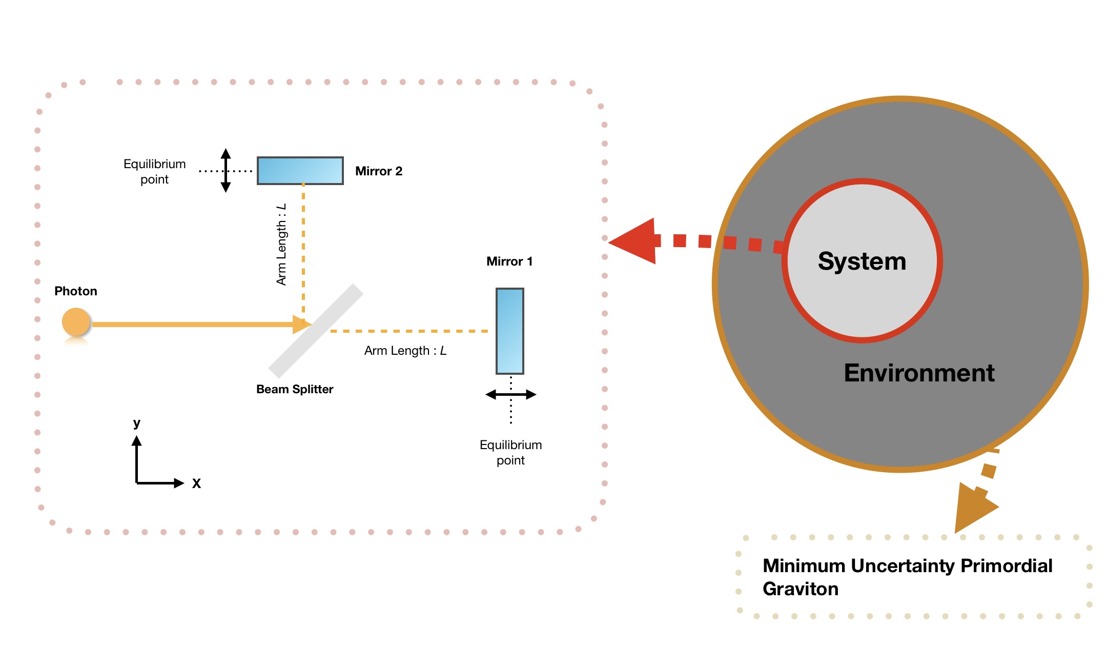
Figure 1: The Michelson equal arm interferometer (the experimental setup $(\rho_{m})$) in the environment filled with graviton originated from the early universe with the minimum uncertainty initial state $(\rho^{\otimes})$.

The density matrix of the system and environment evolves over the time based on the Langevin equation of geodesic deviation of the mirror in the presence of gravitons. Due to the interaction between the mirror and gravitons, the quantum state of the system and the environment will be entangled. This means to obtain the quantum state of the mirror at a certain time, we will trace out the degrees of freedom of the graviton environment from the total density matrix as in Appendix. We will obtain the density matrix of the mirror at a certain time induced by gravitons (for example, we chose the total of the graviton $N=3$ and $\rho_{f}$ to be equation (4.3)) as

$$\rho_{m}(t_{f}) \approx \rho_{11}(t_{i})+\rho_{22}(t_{i})+\Big{(}\exp\Big{\{}\Phi_{Diag\,\,N=3}[\xi_{1},\xi_{2}]\Big{\}}+\exp\Big{\{}\Phi_{Non-Diag\,\,N=3}[\xi_{1},\xi_{2}]\Big{\}}\Big{)}\,\,\rho_{12}(t_{i})$$ (4.7)

$$+\Big{(}\exp\Big{\{}\Phi^{*}_{Diag\,\,N=3}[\xi_{1},\xi_{2}]\Big{\}}+\exp\Big{\{}\Phi^{*}_{Non-Diag\,\,N=3}[\xi_{1},\xi_{2}]\Big{\}}\Big{)}\,\,\rho_{12}(t_{i})$$

The influence of the environmental gravitons will only affect the interference terms of the mirrors. However, unlike research [9], the influence phase functional in this case will be separated into two parts based on the diagonal $\big{(}\Phi_{Diag}[\xi_{1},\xi_{2}]\big{)}$ and non-diagonal $\big{(}\Phi_{Non-Diag}[\xi_{1},\xi_{2}]\big{)}$ terms of the environmental density matrix. The real part of the influence phase functional will be a factor that influences the existence of the interference terms of the matter density matrix. Because the real part is time-dependent, at a certain time the interference terms will disappear. The process of losing the interference terms is known as decoherence. Which is the real part of the influence phase functional is called the decoherence functional and the time when the interference term is zero is called the decoherence time. In this study there will be two influence phase functional as shown in equation (4.7), meaning that there will also be two decoherences functional, each of which will have the form

$$\Gamma_{Diag}(t_{f})=\frac{m^{2}}{8}\int^{t_{f}}_{0}dt\int^{t_{f}}_{0}dt^{\prime}\,\,Tr\Big{(}\hat{S}^{\otimes\dagger}\big{\{}\hat{N}_{ij}(t),\hat{N}_{kl}(t^{\prime})\big{\}}\hat{S}^{\otimes}\,\,\rho^{\otimes}_{Diag}\Big{)}\,\,\Delta(\xi^{i}\xi^{j})(t)\,\,\Delta(\xi^{k}\xi^{l})(t^{\prime})$$ (4.8)

and

$$\Gamma_{Non-Diag\,\,N=3}(t_{f}) = \ln\Bigg{[}\,\,\bigg{|}\bigg{(}\frac{m^{3}}{24}\int^{t_{f}}_{0}dt\int^{t_{f}}_{0}dt^{\prime}\int^{t_{f}}_{0}dt^{\prime\prime}\,\,Tr\bigg{(}\hat{S}^{\otimes\dagger}\Big{\{}\hat{N}_{ij}(t),\big{\{}\hat{N}_{kl}(t^{\prime}),\hat{N}_{mn}(t^{\prime\prime})\big{\}}\Big{\}}$$ (4.9)

$$\times\hat{S}^{\otimes}\,\,\rho^{\otimes}_{Non-Diag\,\,N=3}\bigg{)}\Delta(\xi^{i}\xi^{j})(t)\,\,\Delta(\xi^{k}\xi^{l})(t^{\prime})\,\,\Delta(\xi^{m}\xi^{n})(t^{\prime\prime})\bigg{)}^{-1}\bigg{|}\,\,\Bigg{]}$$

$$\equiv \ln\Big{[}\,\,\big{|}\mathcal{N}(t_{f})\big{|}\Big{]}$$

Here $\Delta(\xi^{i}\xi^{j})(t)=\xi^{i}_{1}(t)\xi^{j}_{1}(t)-\xi^{i}_{2}(t)\xi^{j}_{2}(t)$, that will be determined based on the experimental setup in Figure (1). Equation (4.8) is the decoherence functional that arises due to the influence of the diagonal terms of the environmental density matrix. This expression will apply not only to the diagonal density matrices of equations (4.3) for $N=3$ but to all environmental density matrices of primordial gravitons with only diagonal elements. It is different from equation (4.9), which this expression specifically appears for the non-diagonal density matrices (4.3) with the total graviton particles $N=3$.

The existence of the squeezing operator on both decoherence functionals is due to gravitons in the environment originating from the early universe. Where squeezed formalism will be used, as in research [12, 34]. This formalism is based on the cosmological inflation model, in which the initial quantum state will experience squeezing as the universe expands rapidly. Although this squeezed representation still faces much criticism [41, 42, 43, 44], it is still often used to study quantum states in the early universe. Mathematically, the squeezing process will be represented as a two-mode squeezed operator as follows

$$\hat{S}^{A}(\zeta)=\sum_{\textbf{k},A}\frac{1}{V}\exp\Big{[}\zeta^{*}\,\,\hat{a}^{A}_{\textbf{k}}\hat{a}^{A}_{-\textbf{k}}-\zeta\,\,\hat{a}^{A\dagger}_{\textbf{k}}\hat{a}^{A\dagger}_{-\textbf{k}}\Big{]},$$ (4.10)

with $\zeta\equiv r_{k}e^{i\varphi_{k}}$, where $r_{k}$ and $\varphi_{k}$ is a squeezing and phase angle parameter. In general, the squeezing parameter $r_{k}$ and the phase $\varphi_{k}$ depend on $k$. However, for simplicity, we regard these variables as constant so that the squeezing parameter can have a value of $0\leq r_{k}$ and the phase angle parameter of $0\leq\varphi_{k}\leq 2\pi$. It should be noted that the squeeze parameter $r_{k}$ here is different from the squeeze parameter in the initial state $(\lambda)$ due to the minimum uncertainty.

4.1 Entanglement Initial State of Primordial Graviton

In this section, we will calculate the decoherence functional for the initial state of the graviton environment in which the entanglement state (2.8), and (2.14) is chosen. If expressed in the form of a density matrix with one polarization mode (only mode $\otimes$), the entanglement state will take the form of the equation (4.4) with $\tanh u=0$, or

$$\rho^{\otimes}=\sum_{n=0}^{N}\,\,\frac{1}{2^{N}}\,\,\begin{pmatrix}N\\ n\end{pmatrix}\ket{n}\bra{n}.$$ (4.11)

This density matrix only has diagonal elements. It means in the density matrix equation (4.7), $\exp\big{\{}\Phi_{Non-Diag\,\,N=3}[\xi_{1},\xi_{2}]\big{\}}\approx 0$. So, there will only be one functional decoherence, namely equation (4.8). To calculate the decoherence functional, we will first calculate the two-point anticommutation relation $Tr\Big{(}\hat{S}^{\otimes\dagger}\big{\{}\hat{N}_{ij}(t),\hat{N}_{kl}(t^{\prime})\big{\}}\hat{S}^{\otimes}\rho^{\otimes}\Big{)}$. By using the definition of the noise operator from the graviton in equation (3.8), then

$$Tr\Big{(}\hat{S}^{\otimes\dagger}\big{\{}\hat{N}_{ij}(t),\hat{N}_{kl}(t^{\prime})\big{\}}\hat{S}^{\otimes}\rho^{\otimes}\Big{)} = \frac{\kappa^{2}}{10\pi^{2}}\bigg{(}\delta_{ik}\delta_{jl}+\delta_{il}\delta_{jk}-\frac{2}{3}\delta_{ij}\delta_{kl}\bigg{)}\int_{0}^{\Omega_{m}}\,dk\,\,k^{6}P(t,t^{\prime},k),$$

where $P(t,t^{\prime},k)$, is

$$Tr\bigg{(}\hat{S}^{\otimes\dagger}\big{\{}\hat{h}^{\otimes}_{\textbf{k},I}(t),\hat{h}^{\otimes}_{\textbf{k}^{\prime},I}(t^{\prime})\big{\}}\hat{S}^{\otimes}\rho^{\otimes}\bigg{)}=\delta_{\textbf{k}+\textbf{k}^{\prime},0}P(t,t^{\prime},k).$$ (4.13)

By using the density matrix (4.11) and squeezed operator (4.10), we got

$$P(t,t^{\prime},k) = \frac{(N+1)}{2k}\Big{[}\cos(k(t-t^{\prime}))\cosh 2r_{k}-\cos(k(t-t^{\prime})-\varphi_{k})\sinh 2r_{k}\Big{]}$$ (4.14)

Based on the conventional inflation scenario, $\sinh 2r_{k}\simeq\cosh 2r_{k}\simeq(k_{c}/k)^{4}$, where $k_{c}=2\pi f_{c}$ and $f_{c}$ is the cutoff frequency of primordial gravitational waves. The bound on the cutoff frequency from CMB is $f_{c}\lesssim 10^{9}\,\,$ Hz. Obtained

$$\int_{0}^{\Omega_{m}}\,dk\,\,k^{6}P(t,t^{\prime},k)\approx\Big{(}N+1\Big{)}\,\,k^{4}_{c}\,\,\Omega^{2}_{m}\,\,\frac{x\sin(x)+\cos(x)-1}{x^{2}},$$ (4.15)

with $x=\Omega_{m}(t-t^{\prime})$. Based on the experimental setup in Figure (1), there will be two possible forms of $\Delta(\xi^{i}\xi^{j})(t)$ that are

$$\Delta\xi^{2}_{1}(t) = (L+A\cos\omega t)^{2}-L^{2},$$ (4.16)

$$\Delta\xi^{2}_{2}(t) = L^{2}-(L+A\cos\omega t)^{2}.$$ (4.17)

If the oscillation amplitude is much smaller than the length of the interferometer arm, equation (4.16) and (4.17) can be approximated to be $\Delta\xi^{2}_{i}\sim 2LA$. Substituting equation (4.15) into equation (4.8) and using the same method as in the research [9], then the decoherence functional becomes

$$\Gamma_{Diag}(t_{f})\approx\Big{(}N+1\Big{)}\,\,\frac{4\pi^{3}}{5}\bigg{(}\frac{m}{M_{p}}\bigg{)}^{2}(L\,\,f_{c})^{4}\bigg{(}\frac{A}{L}\bigg{)}^{2}(\omega\,\,t_{f})$$ (4.18)

This decoherence functional is a general form of decoherence functional for the environment in the form of a Bunch-Davies vacuum. Where there will be a factor $(N+1)$, the role of this factor can be seen when we consider the decoherence time $t_{f}$. For $N=0$, the decoherence time (the condition when $\Gamma_{Diag}(t_{f})\simeq 1$) will be 20 seconds when the parameters $\omega=10^{3}$ Hz, $L=40$ km, $m=40$ kg, $f_{c}=10^{9}$ Hz, and $A=10/\sqrt{2m\omega}$ are selected. This means when $N\neq 0$, the bigger the number of $N$, the decoherence time will be reduced to $20/(N+1)$ seconds. However, if you want to maintain the decoherence time for 20 seconds, you can reduce the dimension of the interferometer arm $(L)$ or the mass of the mirror $(m)$ by $(N+1)^{-1/2}$ times.

4.2 Superposition Initial State of Primordial Graviton

This section will calculate the decoherence functional for the environmental density matrix as an equation (4.3) for $N=3$. This density matrix will induce two decoherence functionals. Where the interference terms of the mirror density matrix equation (4.7) will not be zero if one of its decoherence functional values is small ($\Gamma(t_{f})<1$). For the diagonal decoherence functional $(\Gamma_{Diag}(t_{f}))$, the expression is not much different from equation 4.18 for $N=3$ (just replacing the factor $(N+1)$ with $(4-3\tanh^{2}u)$), meaning that the decoherence time of this function will only last for a maximum of 20 seconds. Meanwhile, for the non-diagonal decoherence functional $(\Gamma_{Non-Diag\,\,N=3}(t_{f}))$, different results will be obtained.

To start the discussion, we will calculate the three-point correlation from the non-diagonal decoherence functional of equation (4.9), which will take the following form

$$Tr\bigg{(}\hat{S}^{\otimes\dagger}\Big{\{}\hat{N}_{ij}(t),\big{\{}\hat{N}_{kl}(t^{\prime}),\hat{N}_{mn}(t^{\prime\prime})\big{\}} \Big{\}}\hat{S}^{\otimes}\,\,\rho^{\otimes}_{Non-Diag\,\,N=3}\bigg{)}$$

$$=\frac{\bigg{(}\delta_{ik}\delta_{jl}+\delta_{il}\delta_{jk}-\frac{2}{3}\delta_{ij}\delta_{kl}\bigg{)}}{10\pi^{2}M^{3}_{p}}\,\,\int_{0}^{\Omega_{m}}dk\,\,k^{8}\,\,e^{\otimes}_{\textbf{k},mn}\,\,F(t,t^{\prime},t^{\prime\prime},k),$$ (4.19)

with $F(t,t^{\prime},t^{\prime\prime},k)$ is

$$Tr\bigg{(}\hat{S}^{\otimes\dagger}(\zeta)\Big{\{}\delta\hat{h}^{\otimes}_{\textbf{k},I}(t),\big{\{}\delta\hat{h}^{\otimes}_{\textbf{k}^{\prime},I}(t^{\prime}),\delta\hat{h}^{\otimes}_{\textbf{k}^{\prime\prime},I}(t^{\prime\prime})\big{\}}\Big{\}}\hat{S}^{\otimes}(\zeta)\,\,\rho^{\otimes}_{Non-Diag\,\,N=3}\bigg{)}=\delta_{\textbf{k}-\textbf{k}^{\prime},0}\,\,\delta_{\textbf{k}^{\prime}+\textbf{k}^{\prime\prime},0}\,\,F\,\,(t,t^{\prime},t^{\prime\prime},k)$$ (4.20)

and the polarisation tensor $e^{\otimes}_{\textbf{k},mn}$ will look like [47]

$$e^{A}_{\textbf{k},mn}=\frac{1}{\sqrt{2}}\begin{pmatrix}1&\mp i&0\\ \mp i&1&0\\ 0&0&0\end{pmatrix}.$$ (4.21)

The $\pm$ sign in the matrix refers to the choice of the polarization mode of the primordial gravitational wave. Furthermore, because $\Delta(\xi^{i}\xi^{j})(t)$ is only non-zero when the index $i=j$ as shown in equations (4.16) and (4.17), the part of the polarization tensor that affects the calculation of the three-point correlation function is only the diagonal elements. Taking that $\cosh 3r_{k}\sim(k_{c}/k)^{6}$ we got

$$F(t,t^{\prime},t^{\prime\prime},k) \approx \frac{\sqrt{6}}{12\,\,k^{3/2}}\,\,\tanh u\big{(}1-\tanh^{2}u\big{)}^{1/2}\bigg{[}\bigg{(}\frac{k_{c}}{k}\bigg{)}^{6}\,\,\cos\Big{(}k\big{(}t+t^{\prime}+t^{\prime\prime}\big{)}\Big{)}\bigg{]}$$ (4.22)

then

$$\int_{0}^{\Omega_{m}}dk\,\,k^{8}\,\,e^{\otimes}_{\textbf{k},mn}\,\,F(t,t^{\prime},t^{\prime\prime},k)\approx\frac{\sqrt{6}}{24}\,\,k^{6}_{c}\,\,\tanh u(1-\tanh^{2}u)^{1/2}\,\,\frac{\Omega^{1/2}_{m}\,\,\sin\big{(}\Omega(t+t^{\prime}+t^{\prime\prime})\big{)}}{(t+t^{\prime}+t^{\prime\prime})}.$$ (4.23)

Substituting into equation (4.2) then equation (4.9), using some integration and choosing the UV cutoff $\Omega_{m}\sim\xi^{-1}\equiv L^{-1}$ we find

$$\mathcal{N}(t_{f})^{-1} \approx \frac{3\sqrt{3}m^{2}\pi^{4}}{5M^{3}_{p}}\big{(}A\,\,f^{2}_{c}\big{)}^{3}\,\,\tanh u\big{(}1-\tanh^{2}u\big{)}^{1/2}\bigg{(}\frac{(t_{f}\,\,L^{-1/2})-2L^{3/2}\,\,(4\omega^{2}\,\,t^{2}_{f}+2)}{8\omega^{2}L^{2}-1}\bigg{)}.$$

The non-diagonal decoherence functional can be obtained by calculating the natural logarithm of the absolute value of $\mathcal{N}(t_{f})$. If the same parameters are taken as in section (4.1), then the decoherence time is in the order $\sim\big{(}\tanh u\sqrt{1-\tanh^{2}u}\,\,\big{)}^{-1/2}10^{9}$ second. This result is much longer than the decoherence time from the diagonal decoherence functional. Unless the constant $u\sim 0$ or $\tanh u\sim 1$ (when the non-diagonal density matrix $(\rho^{\otimes}_{Non-Diag})$ vanishes, this condition is met). This means that the interference terms of the mirror density matrix will last much longer because of the non-diagonal terms of the environment density matrix. So, the quantum noise will be able to be detected for a longer period of time. Although this result looks quite long for a decoherence process, based on research by V. A. De Lorenci and L. H. Ford [13], this result is still within the possible decoherence time induced by graviton.

5 Conclusion

This work investigated the decoherence time induced by the noise of graviton from the early universe. The initial state of the graviton is assumed to be the generalization of the Bunch-Davies vacuum, where the initial quantum state is chosen to be in a condition where the measurement accuracy is closest to the classical concept, which is the condition of minimum uncertainty. To obtain an initial state with minimum uncertainty conditions, we use the operators that can define the polarization intensity of gravitational waves, namely the Stoke operator. It is found that the initial state can be an entanglement, or in a more general form, it can be a superposition between the vacuum and the entanglement state. The expression of the initial state in the form of a superposition will cause its density matrix representation to have non-diagonal elements. As we know, the existence of non-diagonal elements is a unique condition in quantum physics that is not possible in the classical concept.

To calculate the decoherence time, we have first looked for the expression of the decoherence functional if the experimental setup of the system is in the same form as S. Kanno et al.’s research [[9]]. Where a Michelson equal arm interferometer, which has two macroscopic suspended mirrors at the end of each interferometer arm, is used. The experimental setup will be in an environment containing gravitons from the early universe. Using the influence functional method and because the initial state of the primordial graviton can have non-diagonal elements, there will be two decoherence functional caused by the diagonal and non-diagonal elements of the initial graviton density matrix. To calculate each functional decoherence, squeezed formalism will be used.

If the initial state of the graviton is entanglement (it has no non-diagonal elements), then there will only be one decoherence functional, such as in the case of the initial state of a Bunch-Davies vacuum. The decoherence functional obtained is similar to the Bunch-Davies vacuum. There will be a factor of $(N+1)$ for the initial entanglement state. This factor can reduce the dimensions of the interferometer arm or the mass of the experimental setup mirror if the decoherence time of the noise of graviton is maintained for 20 seconds (maximum decoherence time for entanglement and Bunch-Davies vacuum initial state). If the initial state is a superposition of the vacuum and entanglement states, then the non-diagonal terms will induce a decoherence functional. Consequently, the decoherence time can last much longer than vacuum or entanglement states, which will be maintained for $\approx 10^{19}$ seconds.

Appendix A Influence Functional Method

This section of the appendix will explain the influence functional method, as in the research [48], for determining the expression of the decoherence functional. However, in this explanation, the environmental density matrix will be assumed to be an equation (4.3) with non-diagonal terms. This appendix will be divided into two parts. The B.1 part will explain the decoherence functional in the QED (quantum electrodynamics) case, and the B.2 part is for the gravity case.

A.1 Influence Functional in QED

Before discussing the decoherence functional for the gravitational case, we first considered the decoherence functional with the same analogy (QED). Suppose a matter $(\rho_{m})$ is in an environment with electromagnetic field radiation. In the initial state, the density matrix can be written as $\rho(t_{i})=\rho_{m}(t_{i})\otimes\rho_{f}(t_{i})$, where $\rho_{f}(t)$ is the environmental density matrix. If we want to calculate the matter density matrix at a final time $\rho_{m}(t_{f})$, then

$$\rho_{m}(t_{f})=Tr_{f}\bigg{(}T_{\leftarrow}\exp\Big{(}\int_{t_{i}}^{t_{f}}d^{4}x\mathcal{L}(x)\Big{)}\rho(t_{i})\bigg{)}.$$ (A.1)

Where $T_{\leftarrow}$ is the time-ordering operator and $\mathcal{L}(x)$ is the Liouville super operator, which has the relation

$$\mathcal{L}(x)\rho=-i[\mathcal{H}(x),\rho]$$ (A.2)

$\mathcal{H}(x)$ denotes the Hamiltonian density at spacetime coordinates $x=x^{\mu}=(x^{0},\vec{x})$. We choose the coulomb gauge in the following, which means that the Hamiltonian density takes the form $\mathcal{H}(x)=\mathcal{H}_{C}(x)+\mathcal{H}_{tr}(x)$, with

$$\mathcal{H}_{C}(x)=\frac{1}{2}\int\,\,d^{3}y\frac{j^{0}(x^{0},\vec{x})j^{0}(x^{0},\vec{y})}{4\pi|\vec{x}-\vec{y}|},$$ (A.3)

and

$$\mathcal{H}_{tr}(x)=j^{\mu}(x)A_{\mu}(x).$$ (A.4)

$\mathcal{H}_{tr}(x)$ represents the Hamiltonian density of the interaction of the matter current density $j^{\mu}(x)$ with the transverse radiation field $A^{\mu}(x)$. Next, the time-ordering operator $T_{\leftarrow}$ will be decomposed into a time-ordering operator $T_{\leftarrow}^{j}$ for matter current and a time-ordering operator $T_{\leftarrow}^{A}$ for electromagnetic fields. With some derivation and defined current super operator $J^{\mu}_{+}(x)\rho\equiv j^{\mu}(x)\rho$ and $J^{\mu}_{-}(x)\rho\equiv\rho j^{\mu}(x)$, then equation (A.1) becomes

$$\rho_{m}(t_{f}) = T^{j}_{\leftarrow}\bigg{(}\exp\bigg{[}\int_{t_{i}}^{t_{f}}d^{4}x\mathcal{L}_{C}(x)-\frac{1}{2}\int_{t_{i}}^{t_{f}}d^{4}x\int_{t_{i}}^{t_{f}}d^{4}x^{\prime}\theta(t-t^{\prime})\,\,[A_{\mu}(x),A_{\nu}(x^{\prime})]J^{\mu}_{+}(x)J^{\nu}_{+}(x^{\prime})$$ (A.5)

$$+\frac{1}{2}\int_{t_{i}}^{t_{f}}d^{4}x\int_{t_{i}}^{t_{f}}d^{4}x^{\prime}\theta(t-t^{\prime})[A_{\mu}(x),A_{\nu}(x^{\prime})]J^{\mu}_{-}(x)J^{\nu}_{-}(x^{\prime})\bigg{]}W[J_{+},J_{-}]\bigg{)}.$$

Where

$$W[J_{+},J_{-}]=Tr_{f}\biggl{\{}\exp\bigg{[}\int_{t_{i}}^{t_{f}}d^{4}x\mathcal{L}_{tr}(x)\rho(t_{i})\bigg{]}\biggr{\}}.$$ (A.6)

This functional is part of the density matrix of matter at any time $(\rho_{m}(t_{f}))$ that contains the correlation between the matter field and electromagnetic radiation. In general, the initial radiation density matrix $\rho_{f}(t_{i})$ will be chosen as a thermal equilibrium state where the density matrix of that state has only diagonal elements. In this study, the environmental state of the graviton is in conditions of minimum uncertainty that allow for non-diagonal elements in the density matrix. So $\rho_{f}(t_{i})$ will be expanded and assumed to be the same as equation (4.3). Furthermore, using an exponential expansion in equation (A.6) is obtained

$$W[J_{+},J_{-}] = Tr_{f}\biggl{\{}\bigg{[}1+\int d^{4}x\mathcal{L}_{tr}(x)+\frac{1}{2!}\int d^{4}x\int d^{4}x^{\prime}\mathcal{L}_{tr}(x)\mathcal{L}_{tr}(x^{\prime})$$ (A.7)

$$+\frac{1}{3!}\int d^{4}x\int d^{4}x^{\prime}\int d^{4}x^{\prime\prime}\mathcal{L}_{tr}(x)\mathcal{L}_{tr}(x^{\prime})\mathcal{L}_{tr}(x^{\prime\prime})+...\,\,\bigg{]}\rho_{m}(t_{i})\otimes\rho_{f}(t_{i})\biggr{\}}$$

The density matrix $\rho_{f}(t_{i})$ in general can be split into a diagonal and a non-diagonal part $\Big{(}\rho_{f}(t)\equiv\rho_{f,Diag}(t)+\rho_{f,Non-Diag}(t)\Big{)}$. If the total particle $N$ is odd, then the diagonal density matrix $\rho_{f,Diag}(t)$ will only work on even-order Liouville super operators, while the non-diagonal density matrix $\rho_{f,Non-Diag}(t)$ will only work on odd-order Liouville super operators. This means that for $N=3$, the functional $W[J_{+},J_{-}]$ can be written as

$$W[J_{+},J_{-}] = \bigg{(}\exp\bigg{[}\frac{1}{2}\int d^{4}x\int d^{4}x^{\prime}\,\,\,\,Tr_{f}\bigg{\{}\mathcal{L}_{tr}(x)\mathcal{L}_{tr}(x^{\prime})\rho_{f,Diag\,\,N=3}(t_{i})\bigg{\}}\bigg{]}$$

$$+\frac{1}{3!}\int d^{4}x\int d^{4}x^{\prime}\int d^{4}x^{\prime\prime}Tr_{f}\biggl{\{}\mathcal{L}_{tr}(x)\mathcal{L}_{tr}(x^{\prime})\mathcal{L}_{tr}(x^{\prime\prime})\rho_{f,Non-Diag\,\,N=3}(t_{i})\biggr{\}}\bigg{)}\rho_{m}(t_{i}).$$

The Liouville super operators with odd orders are limited only to the third. The first term of the equation can be obtained by using the Wick theorem for the Gaussian correlation function, where the even-order correlation function can always be expressed as a two-point correlation function. From this result, if it is substituted back into equation (A.5), and defining a commutator superoperator $J_{c}(x)$

$$J^{\mu}_{c}(x)\rho\equiv[J^{\mu}_{c}(x),\rho]\,\,\,\,\,\,\,\,\,\,\,\,\,\,\,\,\,\,\,\,J^{\mu}_{c}(x)=J^{\mu}_{+}(x)-J^{\mu}_{-}(x)$$ (A.9)

and an anticommutator superoperator $J_{a}(x)$

$$J^{\mu}_{a}(x)\rho\equiv{J^{\mu}_{c}(x),\rho}\,\,\,\,\,\,\,\,\,\,\,\,\,\,\,\,\,\,\,\,J^{\mu}_{a}(x)=J^{\mu}_{+}(x)+J^{\mu}_{-}(x),$$ (A.10)

then we got

$$\rho_{m}(t_{f}) = T^{j}_{\leftarrow}\Big{(}\exp\Big{\{}\Phi_{Diag\,\,N=3}[J_{c},J_{a}]\Big{\}}+\exp\Big{\{}\Phi_{Non-Diag\,\,N=3}[J_{c},J_{a}]\Big{\}}\Big{)}\rho_{m}(t_{i}).$$ (A.11)

$\Phi_{Diag\,\,N=3}[J_{c},J_{a}]$ is the influence phase functional resulting from the diagonal density matrix $\Big{(}\rho_{f,Diag}(t)\Big{)}$ and $\Phi_{Non-Diag\,\,N=3}[J_{c},J_{a}]$ is influence phase functional caused by the no-diagonal density matrix $\Big{(}\rho_{f,Non-Diag}(t)\Big{)}$. Each of those influence phase functional are

$$\Phi_{Diag\,\,N=3} = \int_{t_{i}}^{t_{f}}d^{4}x\mathcal{L}_{C}(x)+\frac{1}{2}\int_{t_{i}}^{t_{f}}d^{4}x\int_{t_{i}}^{t_{f}}d^{4}x^{\prime}\bigg{[}\,\,iD(x-x^{\prime})_{\mu\nu}\,\,J^{\mu}_{c}(x)J^{\nu}_{a}(x^{\prime})$$ (A.12)

$$-Tr_{f}\Big{(}\big{\{}A_{\mu}(x),A_{\nu}(x^{\prime})\big{\}}\,\,\rho_{f,Diag\,\,N=3}(t_{i})\Big{)}J^{\mu}_{c}(x)J^{\nu}_{c}(x^{\prime})\bigg{]}$$

and

$$\Phi_{Non-Diag\,\,N=3} = \int_{t_{i}}^{t_{f}}d^{4}x\mathcal{L}_{C}(x)+\frac{1}{2}\int_{t_{i}}^{t_{f}}d^{4}x\int_{t_{i}}^{t_{f}}d^{4}x^{\prime}\bigg{[}\,\,iD(x-x^{\prime})_{\mu\nu}\,\,\Big{(}J^{\mu}_{c}(x)J^{\nu}_{a}(x^{\prime})$$ (A.13)

$$+J^{\mu}_{a}(x)J^{\nu}_{c}(x^{\prime})\Big{)}\bigg{]}-\ln\Bigg{[}\,\,\bigg{|}\frac{1}{6}\int_{t_{i}}^{t_{f}}d^{4}x\int_{t_{i}}^{t_{f}}d^{4}x^{\prime}\int_{t_{i}}^{t_{f}}d^{4}x^{\prime\prime}\,\,$$

$$\times Tr_{f}\bigg{(}\Big{\{}A_{\mu}(x),\big{\{}A_{\nu}(x^{\prime}),A_{\gamma}(x^{\prime\prime})\big{\}}\Big{\}}\rho_{f,Non-Diag\,\,N=3}(t_{i})\bigg{)}$$

$$\times J^{\mu}_{c}(x)J^{\nu}_{c}(x^{\prime})J^{\gamma}_{c}(x^{\prime\prime})\bigg{|}^{-1}\bigg{]}\pm i\frac{\pi}{2},$$

with $D(x-x^{\prime})_{\mu\nu}\equiv i[A_{\mu(x)},A_{\nu}(x^{\prime})]$. The influence phase functional $\Phi_{Diag\,\,N=3}[J_{c},J_{a}]$ is none other than the influence phase functional that is the same as obtained from the research of H. Breuer and F. Petruccione [48]. When the initial density matrix only has diagonal terms, $\Phi_{Non-Diag\,\,N=3}[J_{c},J_{a}]$ will be zero. The last term in $\Phi_{Non-Diag\,\,N=3}[J_{c},J_{a}]$ appears as a result of the complex logarithm when expressing the second term of equation (A.1) in the form of an exponential.

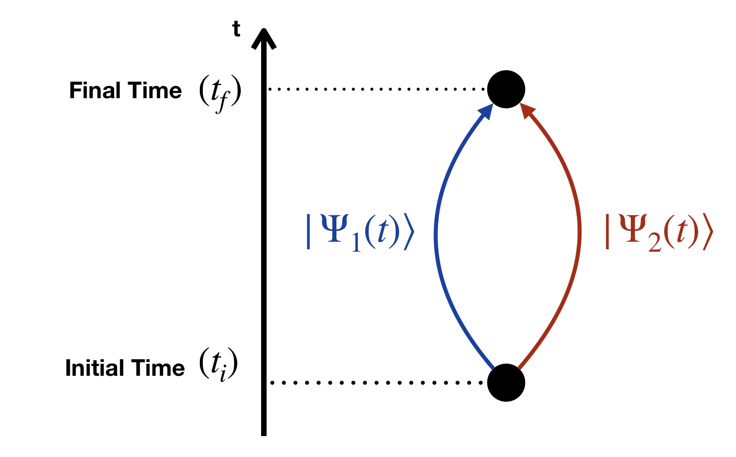
Figure 2: The trajectory of charge particle from initial time $(t_{i})$ into some final time $(t_{f})$.

The matter density matrix must be defined to find the degree of decoherence measurement. Assumed Figure (2) describes the time-dependent quantum state of matter. Where a charged particle in the initial state can transfer to the final state through two trajectories, which will represent two amplitude probabilities (described by two wave packets, $\ket{\Psi_{1}(t)}$ and $\ket{\Psi_{2}(t)}$), then based on the superposition principle, the wave function at the initial time can be written as follows

$$\ket{\Psi(t_{i})}_{m}=\ket{\Psi_{1}(t_{i})}+\ket{\Psi_{2}(t_{i})}.$$ (A.14)

So the density matrix becomes

$$\rho_{m}(t_{i})=\rho_{11}(t_{i})+\rho_{22}(t_{i})+\rho_{12}(t_{i})+\rho_{21}(t_{i}).$$ (A.15)

If $j^{\mu}\ket{\Psi(t)}\approx s^{\mu}(x)\ket{\Psi(t)}$, with $s^{\mu}(x)$ is the classical current density then

$$J^{\mu}_{c}(x)\,\,\rho_{11}\approx J^{\mu}_{c}(x)\,\,\rho_{22}\approx 0,\,\,\,\,\,\,\,\,\,\,\,J^{\mu}_{c}(x)\rho_{12}\approx\big{[}s^{\mu}_{1}(x)-s^{\mu}_{2}(x)\big{]}\,\,\,\,\,\,\,\,\,\,\,J^{\mu}_{a}(x)\rho_{12}\approx\big{[}s^{\mu}_{1}(x)+s^{\mu}_{2}(x)\big{]}$$

and

$$\mathcal{L}_{C}(x)\,\,\rho_{11}\approx\mathcal{L}_{C}(x)\,\,\rho_{22}\approx 0$$ (A.16)

Substituted the matrix density equation (A.15) into equation (A.11) is obtained

$$\rho_{m}(t_{f}) \approx \rho_{11}(t_{i})+\rho_{22}(t_{i})+\Big{(}\exp\Big{\{}\Phi_{Diag\,\,N=3}[s_{1},s_{2}]\Big{\}}+\exp\Big{\{}\Phi_{Non-Diag\,\,N=3}[s_{1},s_{2}]\Big{\}}\Big{)}\,\,\rho_{12}(t_{i})$$ (A.17)

$$+\Big{(}\exp\Big{\{}\Phi^{*}_{Diag\,\,N=3}[s_{1},s_{2}]\Big{\}}+\exp\Big{\{}\Phi^{*}_{Non-Diag\,\,N=3}[s_{1},s_{2}]\Big{\}}\Big{)}\,\,\rho_{12}(t_{i})$$

Where each influence phase functional now becomes

$$\Phi_{Diag\,\,N=3} = \frac{1}{2}\int_{t_{i}}^{t_{f}}d^{4}x\int_{t_{i}}^{t_{f}}d^{4}x^{\prime}\bigg{[}\,\,iD(x-x^{\prime})_{\mu\nu}\,\,\big{[}s^{\mu}_{1}(x)-s^{\mu}_{2}(x)\big{]}\big{[}s^{\nu}_{1}(x^{\prime})+s^{\nu}_{2}(x^{\prime})\big{]}$$

$$-Tr_{f}\Big{(}\big{\{}A_{\mu}(x),A_{\nu}(x^{\prime})\big{\}}\,\,\rho_{f,Diag\,\,N=3}(t_{i})\Big{)}\,\,\big{[}s^{\mu}_{1}(x)-s^{\mu}_{2}(x)\big{]}\big{[}s^{\nu}_{1}(x^{\prime})-s^{\nu}_{2}(x^{\prime})\big{]}\bigg{]}$$

and

$$\Phi_{Non-Diag\,\,N=3} = \frac{1}{2}\int_{t_{i}}^{t_{f}}d^{4}x\int_{t_{i}}^{t_{f}}d^{4}x^{\prime}\Bigg{[}\,\,iD(x-x^{\prime})_{\mu\nu}\,\,\bigg{(}\big{[}s^{\mu}_{1}(x)-s^{\mu}_{2}(x)\big{]}\big{[}s^{\nu}_{1}(x^{\prime})+s^{\nu}_{2}(x^{\prime})\big{]}$$ (A.19)

$$+\big{[}s^{\mu}_{1}(x)+s^{\mu}_{2}(x)\big{]}\big{[}s^{\nu}_{1}(x^{\prime})-s^{\nu}_{2}(x^{\prime})\big{]}\bigg{)}\Bigg{]}-\ln\Bigg{[}\,\,\bigg{|}\frac{1}{6}\int_{t_{i}}^{t_{f}}d^{4}x\int_{t_{i}}^{t_{f}}d^{4}x^{\prime}\int_{t_{i}}^{t_{f}}d^{4}x^{\prime\prime}$$

$$Tr_{f}\bigg{(}\Big{\{}A_{\mu}(x),\big{\{}A_{\nu}(x^{\prime}),A_{\gamma}(x^{\prime\prime})\big{\}}\Big{\}}\,\,\rho_{f,Non-Diag\,\,N=3}(t_{i})\bigg{)}\big{[}s^{\mu}_{1}(x)-s^{\mu}_{2}(x)\big{]}$$

$$\times\big{[}s^{\nu}_{1}(x^{\prime})-s^{\nu}_{2}(x^{\prime})\big{]}\big{[}s^{\gamma}_{1}(x^{\prime\prime})-s^{\gamma}_{2}(x^{\prime\prime})\big{]}\bigg{|}^{-1}\,\,\Bigg{]}\pm\,\,i\frac{\pi}{2}.$$

These two influence phase functionals will only affect the interference terms of the density matrix of the matter. Where the real part of each influence phase functional could suppress the interference terms to be zero, which means there is information that will be lost due to environmental effects (decoherence). Therefore, the real part of those functionals can be defined as decoherence functional. In this case, two decoherence functional will arise as a consequence of the presence of diagonal and non-diagonal terms of the environmental density matrix. Those two decoherences functional can be expressed as follows

$$\Gamma_{Diag}[\,\,\Delta s\,\,]=\frac{1}{2}\int_{t_{i}}^{t_{f}}d^{4}x\int_{t_{i}}^{t_{f}}d^{4}x^{\prime}\,\,Tr_{f}\Big{(}\big{\{}A_{\mu}(x),A_{\nu}(x^{\prime})\big{\}}\,\,\rho_{f,Diag}(t_{i})\Big{)}\,\,\Delta s^{\mu}(x)\Delta s^{\nu}(x^{\prime})$$ (A.20)

and

$$\Gamma_{Non-Diag\,\,N=3}[\,\,\Delta s\,\,] = \ln\Bigg{[}\,\,\bigg{|}\frac{1}{6}\int_{t_{i}}^{t_{f}}d^{4}x\int_{t_{i}}^{t_{f}}d^{4}x^{\prime}\int_{t_{i}}^{t_{f}}d^{4}x^{\prime\prime}\,\,Tr_{f}\bigg{(}\Big{\{}A_{\mu}(x),\big{\{}A_{\nu}(x^{\prime}),A_{\gamma}(x^{\prime\prime})\big{\}}\Big{\}}$$ (A.21)

$$\times\rho_{f,Non-Diag\,\,N=3}(t_{i})\bigg{)}\Delta s^{\mu}(x)\Delta s^{\nu}(x^{\prime})\Delta s^{\gamma}(x^{\prime\prime})\bigg{|}^{-1}\,\,\Bigg{]},$$

where $\Delta s^{\mu}(x)\equiv s^{\mu}_{1}(x)-s^{\mu}_{2}(x)$. For the decoherence functional equation (A.20), because this equation would have the same form for all environment density matrices that only have diagonal elements, the notation $N=3$ is removed.

A.2 Influence Functional in Gravity

Next, we will look for the expression of decoherence functional for the gravity case as in section (3). Where there are two test particles represented in the Fermi coordinates with a quantized gravitational waves environment (graviton). Formally, the expression of decoherence functional will be similar to the QED case. The time evolution that affects the correlation of the system with the environment is induced by a similar interaction Hamiltonian. In the case of gravity, the interaction Hamiltonian can be obtained from the last action term of the equation (3). In the representation of the quantum noise, the interaction Hamiltonian can be expressed as

$$\hat{H}_{int}=-\frac{m}{2}\,\,\hat{N}_{ij}(t)\,\,\hat{\xi}^{i}(t)\hat{\xi}^{j}(t).$$ (A.22)

The two decoherence functionals will be obtained using the same method as the QED case for $N=3$ with the same environmental density matrix. Which could be written as

$$\Gamma_{Diag}(t_{f})=\frac{m^{2}}{8}\int^{t_{f}}_{0}\,\,dt\int^{t_{f}}_{0}\,\,dt^{\prime}\,\,Tr\Big{(}\big{\{}\hat{N}_{ij}(t),\hat{N}_{kl}(t)\big{\}}\,\,\rho^{\otimes}_{Diag}\Big{)}\,\,\Delta(\xi^{i}\xi^{j})(t)\,\,\Delta(\xi^{k}\xi^{l})(t^{\prime})$$ (A.23)

and

$$\Gamma_{Non-Diag\,\,N=3}(t_{f}) = \ln\Bigg{[}\,\,\bigg{|}\frac{m^{3}}{24}\int^{t_{f}}_{0}\,\,dt\int^{t_{f}}_{0}\,\,dt^{\prime}\int^{t_{f}}_{0}\,\,dt^{\prime\prime}\,\,Tr\bigg{(}\Big{\{}\hat{N}_{ij}(t),\big{\{}\hat{N}_{kl}(t^{\prime}),\hat{N}_{mn}(t^{\prime\prime})\big{\}}\Big{\}}$$ (A.24)

$$\times\rho^{\otimes}_{Non-Diag\,\,N=3}\bigg{)}\Delta(\xi^{i}\xi^{j})(t)\,\,\Delta(\xi^{k}\xi^{l})(t^{\prime})\,\,\Delta(\xi^{m}\xi^{n})(t^{\prime\prime})\bigg{|}^{-1}\,\,\Bigg{]},$$

with $\Delta(\xi^{i}\xi^{j})(t)=\xi^{i}_{1}(t)\xi^{j}_{1}(t)-\xi^{i}_{2}(t)\xi^{j}_{2}(t)$, that will be determined based on the experimental setup.

References

- [1] A. Einstein, Sitzungber. Preuss. Akad. Wiss. Berlin, Math. Phys, 688-696 (1916).
- [2] A. Einstein, Sitzungber. Preuss. Akad. Wiss. Berlin, Math. Phys, 154-167 (1918).
- [3] B.P. Abbot et al. [LIGO Scientific and Virgo], Phys. Rev. Lett. 116, 6, 061102 (2016).
- [4] T. Jacobson, Phys. Rev. Lett. 75, 1260-1263 (1995).
- [5] M. Parikh, F. Wilczek and G. Zahariade, International Journal of Modern Physics D, 29(14), 2042001 (2020).
- [6] M. Parikh, F. Wilczek and G. Zahariade, Phys. Rev. Lett. 127, 081602 (2021).
- [7] M. Parikh, F. Wilczek and G. Zahariade, Phys. Rev. D 104, 046021 (2021).
- [8] S. Kanno, J. Soda, and J. Tokuda Phys. Rev. D 103, 044017 (2021).
- [9] S. Kanno, J. Soda, and J. Tokuda Phys. Rev. D 104, 083516 (2021).
- [10] A. Trenggana amd F. P. Zen J. Phys: Conf. Ser. 1949 012005 (2021).
- [11] A. Trenggana amd F. P. Zen J. Phys: Conf. Ser. 2243 012098 (2022).
- [12] D. Maity and S. Pal, Physics Letters B, 835, 137503 (2022).
- [13] V. A. De Lorenci and L. H. Ford Phys. Rev. D 91, 044038 (2015)
- [14] H. T. Cho and B. L. Hu Phys. Rev. D 105 086004 (2022).
- [15] J. Schwinger J. Math. Phys. 2, 407 (1961)
- [16] A. O. Caldeira and A. J. Leggett Phys A (Amsterdam) 121, 587 (1983)
- [17] F. Dyson Is a Graviton Detectable?, Poincare Prize Lecture presented at the International Congress of Mathematical Physics, Aaborg, Denmark, August 6, 2012
- [18] R. Feynman and F. Vernon Ann. Phys. (N.Y.) 24, 118 (1963).
- [19] R. Feynman and A. Hibbs, Quantum Mechanics and Path Integral (1965) McGraw-Hill, Newyork.
- [20] V.I. Dokuchaev, Yu.N. Eroshenko, S.G. Rubin, Astronomy Letters, 35, 143?149 (2009)
- [21] M. F. A. R. Sakti, et al J. Phys: Conf. Ser. 1949, 012016 (2021).
- [22] H. L. Prihadi, M. F. A. R. Sakti, G. Hikmawan and F.P. Zen, Int.J.Mod.Phys.D 29, 2050021 (2020).
- [23] I. Hawke, L. Baiotti, L. Rezzolla and E. Schnetter, Computer Physics Communications 169, 374?377 (2005)
- [24] P. D. Lasky, Publications of the Astronomical Society of Australia (PASA), 32, e034 (2015)
- [25] Y. Watanabe and E. Komatsu, Phys. Rev. D, 73, 123515 (2006).
- [26] L. A. Boyle and P. J. Steinhardt, Phys. Rev. D, 77, 063504 (2008).
- [27] R. Jinno, T. Moroi and K. Nakayama, JCAP, 01 (2014)
- [28] A. A. Starobinsky, Adv. Ser. Astrophys. Cosmol. 3, 130-133 (1987).
- [29] A. A. Starobinsky, Phys. Lett. B 117, 175-178 (1982).
- [30] A. H. Guth, Phys. Rev. D, 23, 347-356 (1981).
- [31] A. D. Linde, Phys. Lett. B 108, 389-393 (1982)
- [32] A. Albrecht and P. J. Steinhardt, Phys. Rev. Lett. 48, 1220-1223 (1982)
- [33] A. D. Linde, Phys. Lett. B 129, 177-181 (1983).
- [34] J. Martin and V. Vennin, Phys. Rev. D 93, 023505 (2016)
- [35] L. Schiff, Quantum Mechanics (1968) Mcgraw-Hill, New York, p. 61.
- [36] G.G. Stokes Trans. Camb. Phil. Soc. 9, 399 (1852).
- [37] H. Nha and J. Kim Physical Review A 74, 012317 (2006).
- [38] C. Aragone, G. Guerri, S. Salamo, and J. L. Tani, J. Phys. A, 7, L149 (1974)
- [39] M. Hillery and L. Mlodinow, Phys. Rev. A 48, 1548 (1993).
- [40] C.Brif and A. Mann, ibid. 54, 4505 (1996).
- [41] C. Kiefer, J. Lesgourgues, D. Polarski and A. A. Starobinsky, Class. Quant. Grav.15, L67 (1998).
- [42] C. Kiefer and D. Polarski, Adv. Sci. Lett. 2, 164 (2009).
- [43] J. T. Hsiang and B. L. Hu Universe 8, 27 (2022).
- [44] I. Agullo, B. Bonga abd P. R. Metidieri Journal of Cosmology and Astroparticle Physics 09, 032 (2022).
- [45] C. C. Gerry, and P. L. Knight, Introductory Quantum Optics, (2005) Cambridge Univ. Press.
- [46] M. Fox, Quantum Optic An Introduction, (2006) Oxford Univ. Press.
- [47] S. Weinberg, Cosmology (1968) Oxford Univ. Press.
- [48] H P Breuer and F Petruccione, Phys. Rev. A 63, 032102 (2001).