ParamNet: A Parameter-variable Network for Fast Stain Normalization

Abstract

In practice, digital pathology images are often affected by various factors, resulting in very large differences in color and brightness. Stain normalization can effectively reduce the differences in color and brightness of digital pathology images, thus improving the performance of computer-aided diagnostic systems. Conventional stain normalization methods rely on one or several reference images, but one or several images are difficult to represent the entire dataset. Although learning-based stain normalization methods are a general approach, they use complex deep networks, which not only greatly reduce computational efficiency, but also risk introducing artifacts. StainNet is a fast and robust stain normalization network, but it has not a sufficient capability for complex stain normalization due to its too simple network structure. In this study, we proposed a parameter-variable stain normalization network, ParamNet. ParamNet contains a parameter prediction sub-network and a color mapping sub-network, where the parameter prediction sub-network can automatically determine the appropriate parameters for the color mapping sub-network according to each input image. The feature of parameter variable ensures that our network has a sufficient capability for various stain normalization tasks. The color mapping sub-network is a fully 1×1 convolutional network with a total of 59 variable parameters, which allows our network to be extremely computationally efficient and does not introduce artifacts. The results on cytopathology and histopathology datasets show that our ParamNet outperforms state-of-the-art methods and can effectively improve the generalization of classifiers on pathology diagnosis tasks. The code has been available at https://github.com/khtao/ParamNet.

Stain normalization, Cytopathology, Histopathology, Convolutional neural network, Generative adversarial network.

1 Introduction

With the development of computer technology, computer-aided diagnosis (CAD) system has received more and more attention, and many automated pathology diagnosis tools have been developed [1, 2, 3, 4]. In practice, however, the pathology images from different medical centers are often very different due to the differences in staining reagent manufacturers, staff operations, and imaging systems [5, 6]. Even within one medical center, there is some variability over time. For pathologists, small color differences will not affect the diagnosis, but larger color differences will affect even pathologists [7]. For CAD systems, even small color differences can affect their reliability [8]. Stain normalization can effectively reduce these differences by normalizing different color distributions to a uniform color distribution, thereby improving the performance of the CAD system [9, 10, 11].

Conventional stain normalization methods rely on one or several reference images to extract color mapping relationships. However, one or several images are difficult to represent the entire dataset [12, 13]. Conventional methods can be mainly divided into two categories, stain matching based methods [14] and stain-separation methods [15, 16, 5, 17, 18]. Stain matching based methods usually match the mean and standard deviation of the source image with the target image in the color space, e.g. LAB [14]. Stain-separation methods try to separate and normalize each staining channel independently in Optical Density (OD) space [15, 16, 5, 17, 18]. It is very difficult to separate each staining channel for some pathology images using multiple stains, such as cytopathology images [13, 19].

With the rise of deep learning, more and more stain normalization methods have adopted deep learning-based methods [20, 21, 22, 23, 24, 25, 26, 27, 28]. These methods can be roughly divided into two categories, one is the pix2pix-based methods [20, 21, 22, 23, 24], another is CycleGAN-based methods [25, 26, 27, 28].

The pix2pix-based methods try to reconstruct the original image from the color transformed image. These color transformation methods include grayscale [20, 21, 22], Hue-Saturation-Value (HSV) [23] and CIEL*a*b* color space [24]. However, the color variation of the source image still affects the reconstructed image. The CycleGAN-based methods generally adopt cycle consistency loss and adversarial loss to learn the color mapping from the real source and target image [25, 26, 27, 28]. By using real source and target images, the image normalized by these methods is very close to the real target image. However, in real data, due to the mismatch in the distribution of the source and target images and the instability of the GAN network, artifacts, abnormal brightness, or distortion often occur in some cases [12, 13, 29]. These phenomena are unacceptable in stain normalization. Some researchers have tried to solve this problem by using additional structures to make the source image and the normalized image consistent in content [30, 31]. These methods include using the segmentation branch to ensure semantic consistency [30] and using additional branches to ensure the content consistency image a special space [31]. However, these methods add extra branches, complicate training, and cannot really guarantee against anomalies.

Because pathology images often contain a large number of pixels, researchers hope to improve the computational efficiency of stain normalization algorithms. Anand et al. [32] optimized the Vahadane [5] method. and Anghel et al. [10] optimized the Macenko [16] method. Zheng et al. [12] proposed to use 1×1 convolution and sparse routing to achieve fast stain normalization. However, the style of the normalized image by this method is formed automatically and cannot be normalized to a specific color distribution. StainNet [13] used distillation learning and 1×1 convolutional neural network to reduce the amount of normalization computation. However, this method relies on the GAN network as a teacher and can only achieve migration between one style and another.

In this work, we propose a parameter-variable stain normalization network, ParamNet, and an adversarial training framework. Our ParamNet contains two sub-networks, a modified resnet18 network as the prediction sub-network and a fully 1×1 convolutional network as the color mapping sub-network, where the prediction sub-network can predict all parameters of the color mapping sub-network at low resolution, and the color mapping sub-network can directly perform stain normalization at the original resolution. The fully 1×1 convolutional color mapping sub-network only contains only two convolutional layers with a total of 59 variable parameters, which allows our network to be extremely computationally efficient and does not introduce artifacts. The prediction sub-network running at low resolution can automatically determine the parameters of the color mapping sub-network according to each input image. So, our ParamNet can perform various stain normalization tasks, including one-to-one stain normalization and multi-to-one stain normalization, in a fast and robust manner. Our adversarial training framework introduces a texture module between ParamNet and the discriminator, which solves the misfit between weak generators and strong discriminators. Further, we validate the effectiveness of the method on datasets containing multiple staining styles.

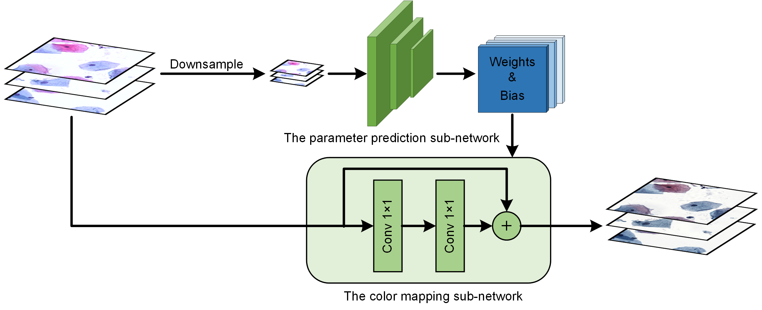
Figure 1: The network structure of ParamNet. First, the parameter prediction sub-network predicts the parameters of the color mapping sub-network at low resolution. Then, the color mapping sub-network uses these parameters to normalize the input image at original resolution.

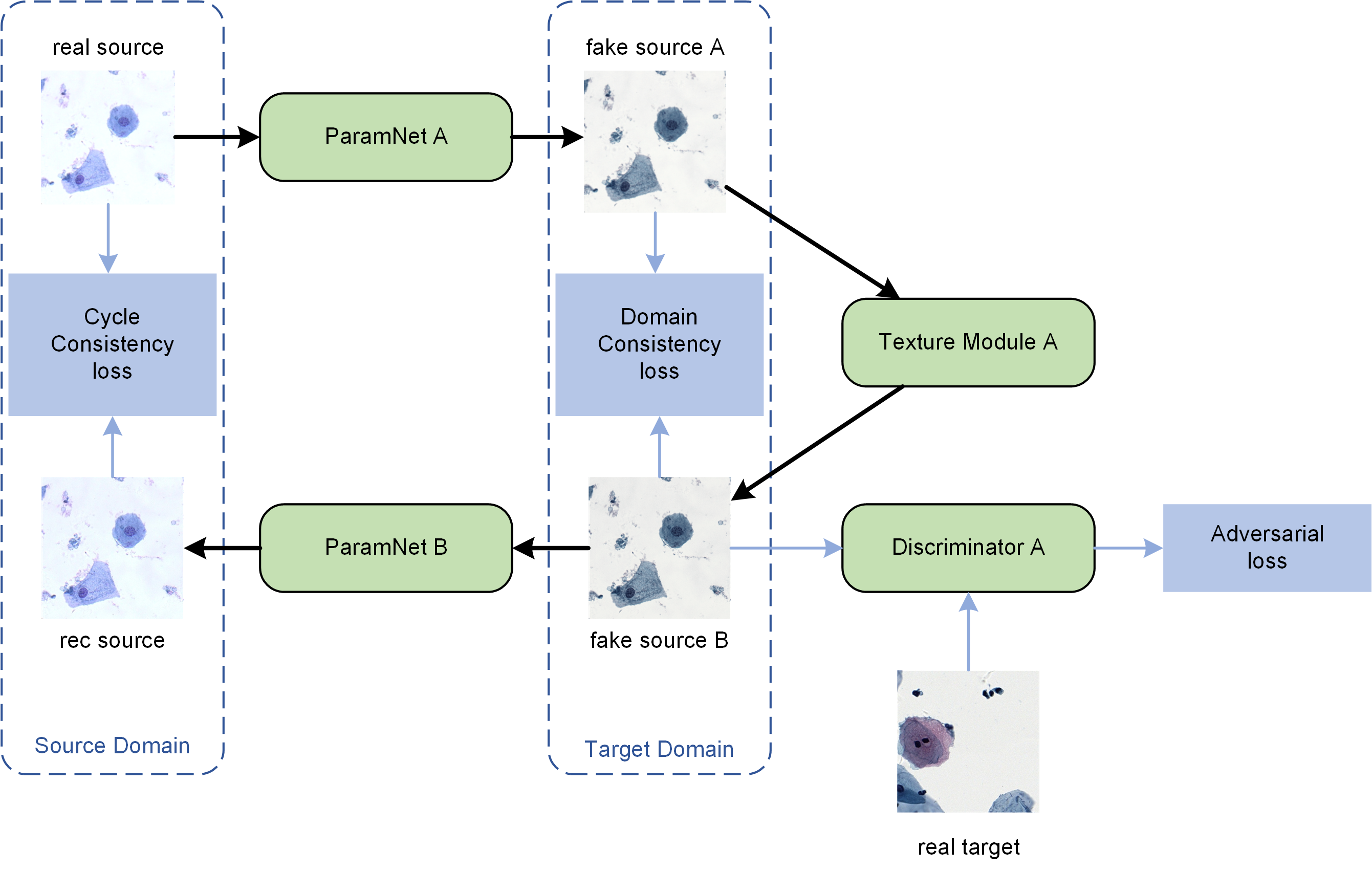
Figure 2: The adversarial training framework of ParamNet. The images from source domain are mapped to the target domain, then add some details and finally back to the source domain. The same reverse process is also performed for the images from the target domain.

2 Methods

In this section, we introduce the network structure of ParamNet and its adversarial training framework.

2.1 The network structure of ParamNet

Stain normalization is an important preprocessing step in CAD system. A practical stain normalization method should have the following features: 1. Fast: Pathological full-slide images usually contain a large number of pixels, so the stain normalization method needs to be computationally efficient. 2. Structural consistency: The stain normalization method should have the same structure as the source image and only change the color style. 3. Multi-domain available: The stain normalization method should be able to normalize the images of multiple color styles at the same time.

StainNet [13] is a fast and robust stain normalization method, but only for one-to-one stain normalization. When normalizing multiple color styles, StainNet [13] has to be trained multiple times to obtain different network parameters. To solve this problem, we propose ParamNet, which can automatically determine the appropriate network parameters for each input image.

As shown in Fig. 1, ParamNet consists of two parts, one is the parameter prediction sub-network, and another is the color mapping sub-network. The parameter prediction sub-network can predict all the parameters of the color map sub-network according to the color style of the input image at low resolution. The color mapping sub-network utilizes these parameters to directly normalize the source image at original resolution. The feature of parameter variable ensures that our network has a sufficient capability for multi-domain normalization.

In our implementation, the parameter prediction sub-network uses a modified resnet18, in which all BatchNorm layers are removed and all convolutional layers are set as biased convolutional layers. For the stability of the network, the output of the prediction sub-network will be normalized by the tanh function, and then multiplied by a learnable parameter. The learnable parameter represents the numerical range of the parameters in the color mapping sub-network and its initial value is set to 4.5. The input image of the parameter prediction sub-network are downsampled to 128×128 by default.

The color mapping sub-network is a fully 1×1 convolutional network, which is same to StainNet [13]. Since only 1×1 convolutional layer is used, our color mapping sub-network only maps a single pixel without interference from the input image’s local neighborhood, thus ensuring the structural consistency of the output image. Relu is used as the activation function of the convolutional layer, and tanh is used as the activation function of the output layer. The color mapping sub-network uses two 1×1 convolutional layers by default, and the number of channels is set to 8. So, the color mapping sub-network only contains 59 variable parameters, which allows our network to be extremely computationally efficient.

2.2 The adversarial training framework of ParamNet

Since ParamNet only transforms the color value of the source image, it retains a lot of information of the source image. In adversarial training, the discriminator can easily distinguish the difference between the image normalized by ParamNet and the real image, resulting in the failure of generating adversarial training. To solve this problem, we introduce a texture module to transform the texture of the output image of ParamNet to obtain an image that can deceive the discriminator.

As shown in Fig. 2, there are two generators (ParamNet A ($G_{A}$) and ParamNet B ($G_{B}$)), two texture modules (Texture Module A ($T_{A}$) and Texture Module B ($T_{B}$)) and two discriminators (Discriminator A ($D_{A}$) and Discriminator B ($D_{B}$)) included in our framework. $G_{A}$ is used to map the images from source domain to target domain, and $G_{B}$ is used to map the images from target domain to source domain. $T_{A}$ is used to add some details to the normalized image by $G_{A}$. $T_{B}$ is used to add some details to the normalized image by $G_{B}$. $D_{A}$ is used to distinguish the difference between the real target image and the output of $T_{A}$, and $D_{B}$ is used to distinguish the difference between the real source image and the output of $T_{B}$.

There are four losses included in our framework, adversarial loss, cycle consistency loss, domain consistency loss and identity loss.

The adversarial loss is used to ensure that the outputs of the two texture modules have the same distribution as the real source and target images. The objective function is defined as:

$$\begin{split}\mathcal{L}_{GAN}(G_{A},T_{A},D_{A})=\mathbb{E}_{t\sim p_{data}(t)}[\|D_{A}(t)\|_{2}]\\ +\mathbb{E}_{s\sim p_{data}(s)}[\|1-D_{A}(T_{A}(G_{A}(s)))\|_{2}],\end{split}$$ (2)

$$\begin{split}\mathcal{L}_{GAN}(G_{B},T_{B},D_{B})=\mathbb{E}_{s\sim p_{data}(s)}[\|D_{B}(s)\|_{2}]\\ +\mathbb{E}_{t\sim p_{data}(t)}[\|1-D_{B}(T_{B}(G_{B}(t)))\|_{2}],\end{split}$$ (3)

where $\|\cdot\|_{2}$ is the $\ell_{2}$-norm, $s$ is the real source image, and $t$ is the real target image.

The cycle consistency loss constrains the consistency of image content by reconstructing the original image from the transformed image. The objective function can be expressed as:

$$\begin{split}\mathcal{L}_{cyc}(G_{A},G_{B},T_{A},T_{B})=\\ \mathbb{E}_{s\sim p_{data}(s)}[\|s-G_{B}(T_{A}(G_{A}(s)))\|_{1}]\\ +\mathbb{E}_{t\sim p_{data}(t)}[\|t-G_{A}(T_{B}(G_{B}(t)))\|_{1}],\end{split}$$ (4)

Domain consistency loss hopes that the texture module changes the image content as little as possible, and only adds some details that can deceive the discriminator. The objective function can be expressed as:

$$\begin{split}\mathcal{L}_{dom}(G_{A},G_{B},T_{A},T_{B})=\\ \mathbb{E}_{s\sim p_{data}(s)}[\|G_{A}(s)-T_{A}(G_{A}(s))\|_{2}]\\ +\mathbb{E}_{t\sim p_{data}(t)}[\|G_{B}(t)-T_{B}(G_{B}(t))\|_{2}],\end{split}$$ (5)

where $\|\cdot\|_{1}$ is the $\ell_{1}$-norm.

Identity loss hopes that when the input image comes from the corresponding target domain, the generator can maintain the identity map without making any changes to the image. Specifically, in this paper, we hope that when the input of $G_{A}$ and $T_{A}$ is from the target domain, $G_{A}$ and $T_{A}$ do not make any changes to the input. Similarly, when the input of $G_{B}$ and $T_{B}$ is from the source domain, $G_{B}$ and $T_{B}$ do not make any changes to the input. The objective function can be expressed as:

$$\begin{split}\mathcal{L}_{ide}(G_{A},G_{B},T_{A},T_{B})=\\ \mathcal{L}_{ide}(G_{A},G_{B})+\mathcal{L}_{ide}(T_{A},T_{B}),\end{split}$$ (6)

$$\begin{split}\mathcal{L}_{ide}(G_{A},G_{B})=\mathbb{E}_{s\sim p_{data}(s)}[\|s-G_{B}(s)\|_{1}]\\ +\mathbb{E}_{t\sim p_{data}(t)}[\|t-G_{A}(t)\|_{1}],\end{split}$$ (7)

$$\begin{split}\mathcal{L}_{ide}(T_{A},T_{B})=\mathbb{E}_{s\sim p_{data}(s)}[\|s-T_{B}(s)\|_{1}]\\ +\mathbb{E}_{t\sim p_{data}(t)}[\|t-T_{A}(t)\|_{1}],\end{split}$$ (8)

In our implementation, the network structure of the texture module and discriminator uses the generator and discriminator in StainGAN [25] respectively.

3 Experiments and Results

3.1 Datasets

In this study, we used four different datasets to verify the performance of different methods, including two public datasets and two private datasets. This study was approved by the Ethics Committee of Tongji Medical College, Huazhong University of Science and Technology. The related descriptions are below:

3.1.1 The aligned cytopathology dataset

The aligned cytopathology dataset from StainNet [13] was used to verify the similarity between the normalized and target images. In this dataset, the same slides (Thinprep cytologic test slides from Hubei Maternal and Child Health Hospital) were scanned using two different scanners. A scanner called Scanner O is equipped with a 20x objective lens with a pixel size of 0.2930um. The other called the Scanner T was equipped with a 40x objective lens with a pixel size of 0.1803. In this dataset, the images from Scanner O and Scanner T are carefully aligned by registration. There are 2257 image pairs in the training set and 966 image pairs in the test set as shown in Table 1. In this study, the images from Scanner O were used as the source images and the images from Scanner T were used as the target images.

3.1.2 The aligned histopathology dataset

The aligned histopathology dataset from StainNet [13] was used to verify the similarity between the normalized and target images. This dataset is originally from the publicly available part of the MITOS-ATYPIA ICPR’14 challenge [33]. This dataset was then aligned, registered, sampled and made publicly available by Kang et al. [13]. In this dataset, the same slides were scanned with two scanners (Aperio Scanscope XT called Scanner A and Hamamatsu Nanozoomer 2.0-HT called Scanner H). Among them, the training set contains 19,200 image pairs, and the test set contains 7,936 image pairs as shown in Table 1. In this study, the images from Scanner A were used as the source images and the images from Scanner H were used as the target images.

Table 1: The number of image pairs on the aligned cytopathology and histopathology dataset.

	training set	test set
The aligned cytopathology dataset	2,257	966
The aligned histopathology dataset	19,200	7,936

Table 2: The number of image patches on the cytopathology and histopathology classification dataset. The classification set is used to train and test the classifier and the stain normalization set is used to train the stain normalization methods.

The cytopathology classification dataset	D1	D2	D3	D4	D5
The classification set	244,341	10,000	10,000	10,000	10,000
The stain normalization set	2,500	625	625	625	625
The histopathology classification dataset	Uni16	C1	C2	C3	C4	C5
The classification set	40,000	13,613	12,355	14,076	9,235	9,696
The stain normalization set	6,000	1,200	1,200	1,200	1,200	1,200

3.1.3 The cytopathology classification dataset

The cytopathology classification dataset is used to verify the performance of the stain normalization algorithm on a multi-domain cytopathology classification diagnostic task. The slides in the cytopathology classification dataset are from Hubei Provincial Maternal and Child Health Hospital and Tongji Hospital. There are five different styles (D1-D5), among which D1-D4 come from Hubei Maternal and Child Health Hospital, and D5 comes from Tongji Hospital. In this dataset, the image patches that contain abnormal cells are labeled as abnormal patches, and the image patches that do not contain any abnormal cells are labeled as normal patches. There are 244,341 image patches in D1 and 40,000 image patches in D2-D5 (10,000 image patches in each center) as shown in Table 2. We randomly picked 2500 image patches in D1 as the target images and 2,500 image patches in D2-D5 as the source images for training the stain normalization algorithm. For the classifier, we use D1 to train the classifier, and use D2-D5 to test the performance of the classifier with and without normalization.

3.1.4 The histopathology classification dataset

The histopathology classification datasets used the publicly available Camelyon16 [34] (399 whole slide images from two centers) and Camelyon17 [35] datasets (1,000 whole slide images from five centers). In our experiments, 100 WSIs from University Medical Center Utrecht (Uni16) in Camelyon16 training part were used to extract the training patches, and 500 WSIs from the five centers (C1-C5) in Camelyon17 training part were used to extract the test patches. In this dataset, the image patches that contain tumor cells are labeled as abnormal patches, and the image patches that do not contain any tumor cells are labeled as normal patches. There are 40,000 image patches from Uni16 in the training set of this dataset. And there are 58,975 image patches in the test set of this dataset as shown in Table 2. We randomly picked 6000 image patches from the training set as the target images and 6000 image patches from the test set as the source images for training stain normalization algorithms. For the classifier, we use the training set to train the classifier, and use the test set to test the performance of the classifier with and without normalization.

3.2 Evaluation Metrics

In order to evaluate different methods fairly and effectively, we evaluated different methods in four aspects: similarity with target image, preservation of source image information, computational efficiency, and classifier accuracy.

In order to effectively measure the similarity to the target image and preserve the information of the source image, we use two similarity matrices, Structural Similarity index (SSIM) [36] and Peak Signal-to-Noise Ratio (PSNR). The similarity between the normalized image and the target image is evaluated using SSIM and PSNR, which are denoted as SSIM Target and PSNR Target. The preservation of source image information is evaluated using SSIM, which is denoted as SSIM Source. SSIM Target and PSNR Target are calculated using raw RGB values. Similar to [11,27], SSIM Source is calculated using grayscale images. And the statistic results of SSIM Target, PSNR Target, and SSIM Source on the testing set in the aligned cytopathology dataset and the aligned histopathology dataset are shown in Tables 3 and 4, as Mean ± standard deviation.

In order to evaluate the computational efficiency of different methods, the frames per second (FPS) was calculated on the system with 6-core Intel(R) Core (TM) i7-6850K CPU and NVidia GeForce GTX 1080Ti. And the input and output (IO) time is not included. The FPS results of different methods are shown in Table 5 when the input image size is 512×512.

The accuracy is used to evaluate the classifier performance. The statistic results of accuracy on the cytopathology and histopathology classification datasets are shown in Table 6 and 7, as Mean ± standard deviation.

3.3 Implementation

For conventional methods (Reinhard [14], Macenko [16], Vahadane [5] and GCTI-SN [18]), one professionally selected image is used as the reference image. For the GAN based methods (SAASN [28], StainGAN [25], and StainNet [13]), we use their default training settings.

For ParamNet, there are four losses included in the training framework. During training, we randomly transform image resolutions (0.5 1.0) to stabilize training. We use adam to optimize the network, and the learning rate is linearly increased from 0 to 2e-4 in the first 1000 iterations, and then linearly decreased to 0 until the end of training. We train ParamNet 200k iterations on the aligned cytopathology dataset and aligned histopathology dataset, and 400k iterations on the cytopathology classification dataset and histopathology classification dataset.

For the classifier, we used SqueezeNet [37] pre-trained on ImageNet [38] as the classification network. The classifier was trained using cross entropy loss and adam optimizer. The initial learning rate was set to 0.0002, and it reduced by a factor of 0.1 at the 40th and 50th epoch. The training was stopped at the 60th epoch, which was chosen experimentally. The experiment was repeated 10 times in order to enhance reliability.

3.4 Results

In this section, we compared our method with state-of-art normalization methods, including Reinhard [14], Macenko [16], Vahadane [5], GCTI-SN [18], SAASN [28], StainGAN [25], and StainNet [13].

3.4.1 One-to-One Stain Normalization

In this section, we compare our ParamNet with state-of-art normalization methods on the one-to-one stain normalization task. We report the following results on the aligned cytopathology dataset and the aligned histopathology dataset: (1)Visual comparison among different methods. (2) Quantitative comparison of similarities among different methods. (3) Quantitative comparison of computational efficiency among different methods.

Visual comparison

Firstly, we compared our ParamNet with other stain normalization methods in the visual appearance. The visual comparison among different methods is shown in Fig. 3,4.

The results on the aligned cytopathology dataset are shown in Fig. 3. On the aligned cytopathology dataset, there are 2,257 image pairs in the training set and 966 image pairs in the test set, the images from Scanner O are taken as the source images and the images from Scanner T are taken as the target images. For conventional methods (Reinhard, Macenko, Vahadane and GCTI-SN), the normalized images are far from the target image in color and brightness in Fig. 3. The conventional methods only extract information from a single reference image. Moreover, it is difficult to extract the precise color mapping relationship in this way, resulting in poor performance of the normalized results. For the image normalized by SAASN in Fig. 3, its brightness is closer to the source image than to the target image. The images normalized by StainGAN, StainNet and ParamNet are very close to the target image in Fig. 3. However, in terms of image content, the image normalized by StainGAN has a more complex background, while the image StainNet has a simpler background, only the image normalized by ParamNet is closest to the source image. StainGAN uses a complex convolutional network that tends to introduce additional noise. StainNet uses a single 1×1 convolutional network, which makes it not capable enough to handle complex color mapping relationships. For ParamNet, the ParamNet network it uses can automatically determine the best parameters for each input, thus achieving better performance.

The results on the aligned histopathology dataset are shown in Fig. 4. On the aligned histopathology dataset, there are 19,200 image pairs in the training set and 7,936 image pairs in the test set, the images from Scanner A are taken as the source images and the images from Scanner H are taken as the target images. For conventional methods (Reinhard, Macenko, Vahadane and GCTI-SN), there are still some differences between the normalized image and the target image in color and brightness in Fig. 4. However, the performance of conventional methods on aligned histopathology datasets is significantly better than that on aligned cytopathology datasets. This is because most of the conventional methods are designed for histopathology images and are not suitable for cytopathology images. For the image normalized by SAASN in Fig. 4, its color is lighter to the target image. StainGAN introduces additional noise to the normalized image in Fig. 4. And the images normalized by StainNet and ParamNet are very close to the target image in Fig. 4.

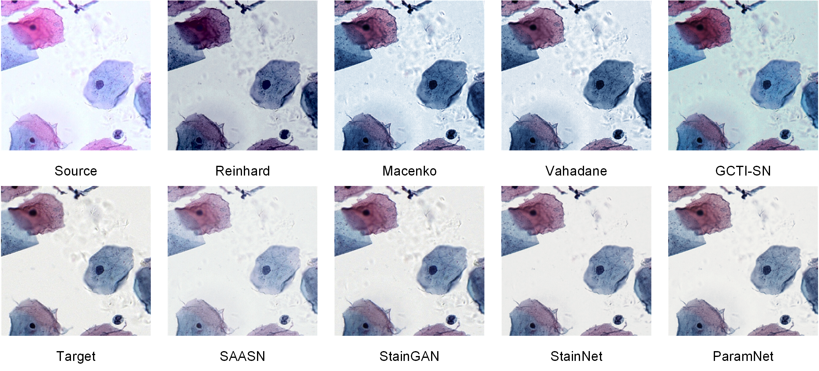
Figure 3: The visual comparison among different methods on the aligned cytopathology dataset.

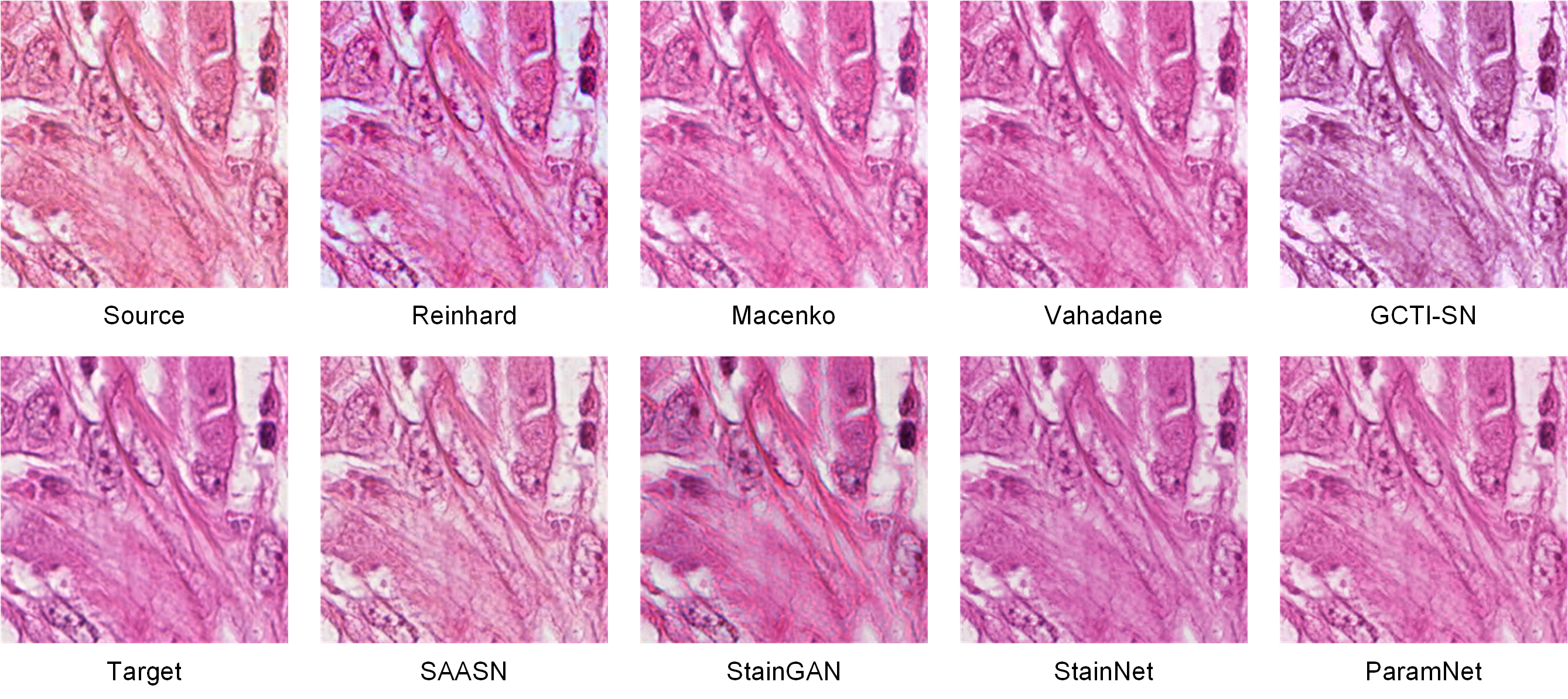
Figure 4: The visual comparison among different methods on the aligned histopathology dataset.

Quantitative comparison of similarities

Secondly, we quantitatively compared our ParamNet with other stain normalization methods in the similarities (the similarity to the target image and the similarity to the source image). The quantitative comparison among different methods is shown in Table 3,4.

The results on the aligned cytopathology dataset are shown in Table 3. The conventional methods (Reinhard, Macenko, Vahadane and GCTI-SN) have low SSIM Target and PSNR Target in Table 3, which means that there is a large difference between the images normalized by the conventional methods and the target images. SAASN has the highest SSIM Source but low PSNR Target, which means that it preserves the information of the source images as much as possible but ignores the similarity with the target images. But the purpose of stain normalization is to be similar to the target images, so SAASN is inappropriate for stain normalization. StainGAN, StainNet and ParamNet have high PSNR Target in Table 3, which means that the images normalized by them are similar enough to the target images. Among these three methods, StainGAN has the lowest SSIM Source, which means it may lose some information of the source images. For our ParamNet, it has the highest PSNR Target and also has a high SSIM Source, which means that it can achieve a high similarity to the target images while preserving the source images information as much as possible.

The results on the aligned histopathology dataset are shown in Table 4. The conventional methods (Reinhard, Macenko, Vahadane and GCTI-SN) have lower SSIM Target and PSNR Target than the GAN based methods (SAASN, StainGAN, StainNet and ParamNet) in Table 4, which means that the GAN based methods can achieve better performance. Among the GAN based methods, SAASN has the highest SSIM Source and the lowest PSNR Target, StainGAN and ParamNet have the highest PSNR Target, and ParamNet has the second highest SSIM Source. So, our ParamNet can achieve a high similarity to the target images while preserving the source images information as much as possible on the aligned histopathology dataset.

Table 3: Different evaluation metrics are reported for various stain normalization methods on the aligned cytopathology dataset.

Methods	SSIM Target	PSNR Target	SSIM Source
Reinhard	0.739±0.046	19.8±3.3	0.885±0.042
Macenko	0.731±0.054	22.5±3.1	0.853±0.054
Vahadane	0.739±0.050	22.6±3.0	0.867±0.050
GCTI-SN	0.764±0.039	19.7±2.7	0.905±0.034
SAASN	0.778±0.026	21.5±2.0	0.990±0.001
StainGAN	0.764±0.030	29.7±1.6	0.905±0.021
StainNet	0.809±0.027	29.8±1.7	0.945±0.025
ParamNet	0.816±0.026	30.0±1.6	0.951±0.023

Table 4: Different evaluation metrics are reported for various stain normalization methods on the aligned histopathology dataset.

Methods	SSIM Target	PSNR Target	SSIM Source
Reinhard	0.617±0.106	19.9±2.1	0.964±0.031
Macenko	0.656±0.115	20.7±2.7	0.966±0.049
Vahadane	0.664±0.116	21.1±2.8	0.967±0.046
GCTI-SN	0.638±0.100	19.7±2.2	0.947±0.043
SAASN	0.690±0.114	21.6±3.5	0.994±0.002
StainGAN	0.706±0.099	22.7±2.6	0.912±0.025
StainNet	0.691±0.107	22.5±3.3	0.957±0.007
ParamNet	0.687±0.106	22.7±3.0	0.966±0.001

Quantitative comparison of computational efficiency

Finally, we quantitatively compared the computational efficiency of our method with other stain normalization methods. We tested the FPS of different methods with an input image size of 512×512 and show in Table 5. As shown in Table 5, our ParamNet (1605.2 FPS) is much faster than StainNet (881.8 FPS), which means that our ParamNet can normalize an 100,000×100,000 whole slide image (WSI) within 25s. The prediction sub-network of ParamNet computes at low resolution and the sub-network of ParamNet computes at high resolution. The sub-network has only two 1×1 convolutional layers with 8 channels, however, StainNet has three 1×1 convolutional layers with 32 channels. So our ParamNet is computationally more efficient than StainNet.

Table 5: Quantitative comparison of computational efficiency among different methods. The input and output (IO) time is not included. The input image size is 512×512.

Methods	Reinhard	Macenko	Vahadane	GCTI-SN	SAASN	StainGAN	StainNet	ParamNet
FPS	54.8	4.0	0.5	6.4	5.2	19.6	881.8	1605.2

3.4.2 Multi-to-One Stain Normalization

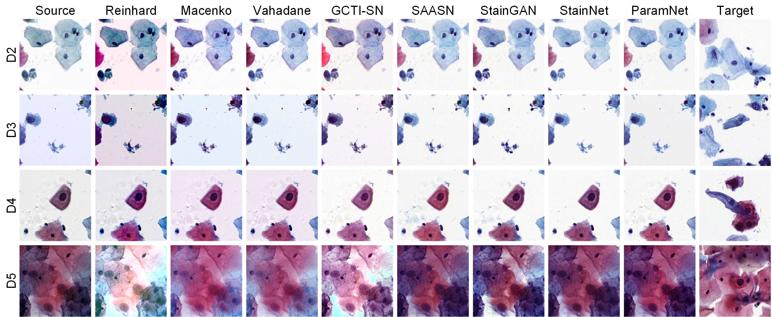
Figure 5: The visual comparison among different methods on the cytopathology classification dataset. The source images have multiple styles (D2-D5), and the target images are from D1.

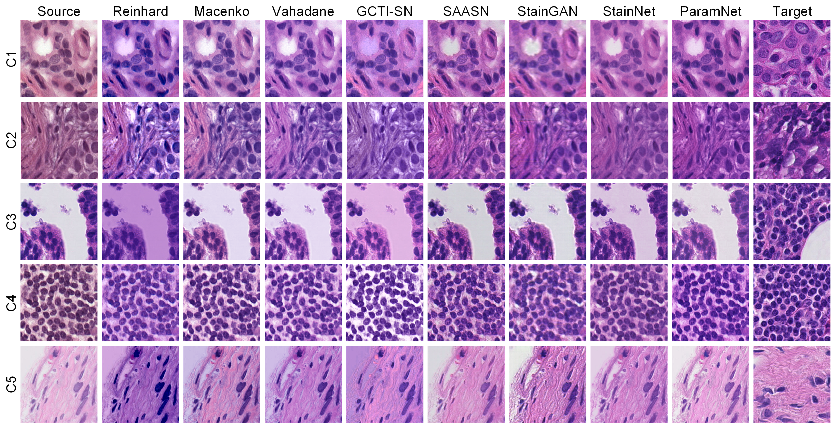
Figure 6: The visual comparison among different methods on the histopathology classification dataset. The source images are from five centers (C1-C5) of Camelyon17, and the target images are from Uni16 of Camelyon16. The source images of C3 and the target images are from same center but at different times.

Table 6: The accuracy for various stain normalization methods on the cytopathology classification dataset.

Accuracy	D2	D3	D4	D5	Average
Original	0.853±0.031	0.915±0.022	0.873±0.029	0.688±0.033	0.832±0.029
Reinhard	0.862±0.015	0.867±0.025	0.796±0.026	0.728±0.025	0.813±0.023
Macenko	0.929±0.014	0.937±0.023	0.915±0.010	0.818±0.034	0.900±0.020
Vahadane	0.905±0.022	0.940±0.031	0.907±0.019	0.745±0.037	0.875±0.026
GCTI-SN	0.932±0.016	0.944±0.022	0.924±0.017	0.850±0.039	0.912±0.024
SAASN	0.964±0.013	0.911±0.024	0.944±0.010	0.863±0.039	0.920±0.022
StainGAN	0.918±0.007	0.908±0.011	0.867±0.006	0.799±0.018	0.873±0.011
StainNet	0.928±0.034	0.963±0.014	0.924±0.032	0.820±0.059	0.909±0.035
ParamNet	0.968±0.013	0.965±0.017	0.943±0.006	0.867±0.039	0.936±0.019

Table 7: The accuracy for various stain normalization methods on the histopathology classification dataset.

Accuracy	C1	C2	C3	C4	C5	Average
Original	0.500±0.016	0.561±0.030	0.907±0.003	0.528±0.014	0.765±0.041	0.652±0.021
Reinhard	0.871±0.014	0.855±0.008	0.815±0.006	0.823±0.027	0.808±0.015	0.834±0.014
Macenko	0.814±0.009	0.832±0.009	0.816±0.007	0.836±0.012	0.789±0.010	0.817±0.009
Vahadane	0.817±0.005	0.826±0.005	0.762±0.007	0.890±0.004	0.805±0.003	0.820±0.005
GCTI-SN	0.840±0.006	0.832±0.007	0.816±0.007	0.879±0.005	0.804±0.006	0.834±0.006
SAASN	0.883±0.004	0.887±0.002	0.908±0.003	0.888±0.004	0.819±0.010	0.877±0.005
StainGAN	0.898±0.004	0.871±0.001	0.921±0.003	0.903±0.004	0.881±0.005	0.895±0.003
StainNet	0.898±0.006	0.836±0.006	0.895±0.005	0.862±0.019	0.877±0.005	0.874±0.008
ParamNet	0.920±0.003	0.857±0.007	0.924±0.003	0.899±0.004	0.884±0.003	0.897±0.004

Firstly, we compared our ParamNet with other stain normalization methods in the visual appearance as shown in Fig. 5,6.

The results on the cytopathology classification dataset are shown in Fig. 5. On the cytopathology classification dataset, there are 2,500 image patches from D2-D5 as the source images and 2,500 image patches from D1 as the target images to train the GAN based methods (SAASN, StainGAN, StainNet and ParamNet). As shown in Fig. 5, there are many wrong variations in color and brightness on the normalized images by the conventional methods (Reinhard, Macenko, Vahadane and GCTI-SN). For example, the cell in the source image of D2 is incorrectly normalized from dark red to bright red by GCTI-SN, and the brightness of the D5’s source image is over-enhanced by Reinhard and GCTI-SN. StainGAN and SAASN use complex convolutional networks for stain normalization, which not only reduces the computational efficiency of the algorithm but also brings artifacts to the normalized image. For example, SAASN and StainGAN add extra contents to the normalized images that do not belong to the source images in D3 and D4. And StainGAN removes some contents belonging to the source image in the normalized image of D5. As for StainNet, it has a single three-layer 1×1 convolutional network, which limits its color-mapping capability. So, there are many details missing, especially on the background of the normalized image by StainNet. Unlike StainNet, our ParamNet uses a variable-parameter 1×1 convolutional network for color mapping, so our ParamNet performs well on the multi-to-one stain normalization task.

The results on the histopathology classification dataset are shown in Fig. 6. On the histopathology classification dataset, there are 6,000 image patches from Camelyon17 (C1-C5) as the source images and 6,000 image patches from Uni16 as the target images to train the GAN based methods (SAASN, StainGAN, StainNet and ParamNet). As shown in Fig. 6, the conventional methods perform better on histopathology images, but there are still many wrong variations in color and brightness. For example, the light background in the source image of center3 is incorrectly normalized to the purple background by Reinhard and GCTI-SN, and the brightness of the center5’s source image is over-enhanced by Macenko and Vahadane. The GAN based methods all show good performance in Fig. 6. However, the normalized images by StainGAN are a little blurry and the normalized images by StainNet are a bit purple. Our ParamNet can achieve the best performance among the GAN based methods.

3.4.3 Application results on the classification task

Moreover, we compared our ParamNet with other stain normalization methods on the classification task. The accuracy for various stain normalization methods is shown in Table 6,7.

The accuracy for various stain normalization methods on the cytopathology classification dataset is shown in Table 6. On the cytopathology classification dataset, we train the classifier with 244,341 image patches from D1 and test the classifier with 40,000 image patches from D2-D5. As shown in Table 6, the classifier has poor performance on the original image of D2-D5, and the classifier has different performance improvements on the images normalized by different methods (except Reinhard). Among conventional methods, the classifier has the best accuracy (0.912 on average) on the images normalized by GCTI-SN. And among GAN based methods, the classifier has the best accuracy (0.936 on average) on the images normalized by our ParamNet. StainGAN and StainNet do not get competitive performance on the cytopathology classification dataset.

The accuracy for various stain normalization methods on the histopathology classification dataset is shown in Table 7. On the histopathology classification dataset, we train the classifier with 40,000 image patches from Uni16 and test the classifier with 58,975 image patches from C1-C5. As shown in Table 7, the classifier has poor performance on the original images of C1-C5, even the accuracy of the classifier is close to 0.5 in C1, C2 and C4. Overall, using the normalized images can significantly improve the performance of the classifier compared to the original images. On the histopathology classification dataset, the classifier has better performance on images normalized by the GAN-based methods than the conventional methods. Among all the normalization methods in Table 7, our method has the highest accuracy (0.897 on average). The images in C3 and Uni16 are from the same medical center but at different times. For the classifier trained on Uni16, the accuracy is 0.907 on the original images of C3. And the accuracy can be increased to 0.924 on the normalized images by our ParamNet, which shows that our method can improve the accuracy of the classifier, even on images from the same center.

4 Discussion and Conclusion

In this paper, we proposed a novel stain normalization network, ParamNet, and an adversarial training framework. ParamNet contains two sub-networks, a modified resnet18 network as the prediction sub-network and a fully 1×1 convolutional network as the color mapping sub-network, where the prediction sub-network can predict all parameters of the color mapping sub-network at a low resolution and the color mapping sub-network can directly normalize the source images at the original resolution. Moreover, we validated the effectiveness of our method on four datasets, the results show that ParamNet has better performance than other methods.

The feature of parameter variable ensures that our network has a sufficient capability for multi-domain normalization. And the color mapping sub-network has an extremely concise network structure, which allows our network to be extremely computationally efficient and does not introduce artifacts. However, since different input images correspond to different parameters, there will be slight inconsistencies between adjacent image blocks. We hope to solve this problem in further study.

References

- [1] J. Tang, R. M. Rangayyan, J. Xu, I. E. Naqa, and Y. Yang, “Computer-aided detection and diagnosis of breast cancer with mammography: Recent advances,” IEEE Transactions on Information Technology in Biomedicine, vol. 13, no. 2, pp. 236–251, 2009.
- [2] Z. Zhang, R. Srivastava, H. Liu, X. Chen, L. Duan, D. W. Kee Wong, C. K. Kwoh, T. Y. Wong, and J. Liu, “A survey on computer aided diagnosis for ocular diseases,” BMC medical informatics and decision making, vol. 14, no. 1, pp. 1–29, 2014.
- [3] S. Cheng, S. Liu, J. Yu, G. Rao, Y. Xiao, W. Han, W. Zhu, X. Lv, N. Li, J. Cai, et al., “Robust whole slide image analysis for cervical cancer screening using deep learning,” Nature communications, vol. 12, no. 1, p. 5639, 2021.
- [4] S. H. Jo, Y. Kim, Y. B. Lee, S. S. Oh, and J.-r. Choi, “A comparative study on machine learning-based classification to find photothrombotic lesion in histological rabbit brain images,” Journal of Innovative Optical Health Sciences, vol. 14, no. 06, p. 2150018, 2021.
- [5] A. Vahadane, T. Peng, A. Sethi, S. Albarqouni, L. Wang, M. Baust, K. Steiger, A. M. Schlitter, I. Esposito, and N. Navab, “Structure-preserving color normalization and sparse stain separation for histological images,” IEEE transactions on medical imaging, vol. 35, no. 8, pp. 1962–1971, 2016.
- [6] A. Bentaieb and G. Hamarneh, “Adversarial stain transfer for histopathology image analysis,” IEEE Transactions on Medical Imaging, vol. 37, no. 3, pp. 792–802, 2018.
- [7] S. M. Ismail, A. B. Colclough, J. S. Dinnen, D. Eakins, D. M. Evans, E. Gradwell, J. P. O’Sullivan, J. M. Summerell, and R. G. Newcombe, “Observer variation in histopathological diagnosis and grading of cervical intraepithelial neoplasia.,” BMJ, vol. 298, no. 6675, pp. 707–710, 1989.
- [8] F. Ciompi, O. Geessink, B. E. Bejnordi, G. S. de Souza, A. Baidoshvili, G. Litjens, B. van Ginneken, I. Nagtegaal, and J. van der Laak, “The importance of stain normalization in colorectal tissue classification with convolutional networks,” in 2017 IEEE 14th International Symposium on Biomedical Imaging (ISBI 2017), pp. 160–163, 2017.
- [9] S. Cai, Y. Xue, Q. Gao, M. Du, G. Chen, H. Zhang, and T. Tong, “Stain style transfer using transitive adversarial networks,” in Machine Learning for Medical Image Reconstruction (F. Knoll, A. Maier, D. Rueckert, and J. C. Ye, eds.), (Cham), pp. 163–172, Springer International Publishing, 2019.
- [10] A. Anghel, M. Stanisavljevic, S. Andani, N. Papandreou, J. H. Rüschoff, P. Wild, M. Gabrani, and H. Pozidis, “A high-performance system for robust stain normalization of whole-slide images in histopathology,” Frontiers in medicine, vol. 6, p. 193, 2019.
- [11] A. M. Khan, N. Rajpoot, D. Treanor, and D. Magee, “A nonlinear mapping approach to stain normalization in digital histopathology images using image-specific color deconvolution,” IEEE transactions on Biomedical Engineering, vol. 61, no. 6, pp. 1729–1738, 2014.
- [12] Y. Zheng, Z. Jiang, H. Zhang, F. Xie, D. Hu, S. Sun, J. Shi, and C. Xue, “Stain standardization capsule for application-driven histopathological image normalization,” IEEE journal of biomedical and health informatics, vol. 25, no. 2, pp. 337–347, 2020.
- [13] H. Kang, D. Luo, W. Feng, S. Zeng, T. Quan, J. Hu, and X. Liu, “Stainnet: a fast and robust stain normalization network,” Frontiers in Medicine, vol. 8, p. 746307, 2021.
- [14] E. Reinhard, M. Adhikhmin, B. Gooch, and P. Shirley, “Color transfer between images,” IEEE Computer graphics and applications, vol. 21, no. 5, pp. 34–41, 2001.
- [15] A. C. Ruifrok, D. A. Johnston, et al., “Quantification of histochemical staining by color deconvolution,” Analytical and quantitative cytology and histology, vol. 23, no. 4, pp. 291–299, 2001.
- [16] M. Macenko, M. Niethammer, J. S. Marron, D. Borland, J. T. Woosley, X. Guan, C. Schmitt, and N. E. Thomas, “A method for normalizing histology slides for quantitative analysis,” in 2009 IEEE international symposium on biomedical imaging: from nano to macro, pp. 1107–1110, IEEE, 2009.
- [17] M. Salvi, N. Michielli, and F. Molinari, “Stain color adaptive normalization (scan) algorithm: Separation and standardization of histological stains in digital pathology,” Computer methods and programs in biomedicine, vol. 193, p. 105506, 2020.
- [18] A. Gupta, R. Duggal, S. Gehlot, R. Gupta, A. Mangal, L. Kumar, N. Thakkar, and D. Satpathy, “Gcti-sn: Geometry-inspired chemical and tissue invariant stain normalization of microscopic medical images,” Medical Image Analysis, vol. 65, p. 101788, 2020.
- [19] G. Gill, Cytopreparation: principles & practice, vol. 12. Springer Science & Business Media, 2012.
- [20] H. Cho, S. Lim, G. Choi, and H. Min, “Neural stain-style transfer learning using gan for histopathological images,” arXiv preprint arXiv:1710.08543, 2017.
- [21] X. Chen, J. Yu, S. Cheng, X. Geng, S. Liu, W. Han, J. Hu, L. Chen, X. Liu, and S. Zeng, “An unsupervised style normalization method for cytopathology images,” Computational and Structural Biotechnology Journal, vol. 19, pp. 3852–3863, 2021.
- [22] P. Salehi and A. Chalechale, “Pix2pix-based stain-to-stain translation: A solution for robust stain normalization in histopathology images analysis,” in 2020 International Conference on Machine Vision and Image Processing (MVIP), pp. 1–7, IEEE, 2020.
- [23] D. Tellez, G. Litjens, P. Bándi, W. Bulten, J.-M. Bokhorst, F. Ciompi, and J. Van Der Laak, “Quantifying the effects of data augmentation and stain color normalization in convolutional neural networks for computational pathology,” Medical image analysis, vol. 58, p. 101544, 2019.
- [24] F. G. Zanjani, S. Zinger, B. E. Bejnordi, J. A. van der Laak, and P. H. de With, “Stain normalization of histopathology images using generative adversarial networks,” in 2018 IEEE 15th International symposium on biomedical imaging (ISBI 2018), pp. 573–577, IEEE, 2018.
- [25] M. T. Shaban, C. Baur, N. Navab, and S. Albarqouni, “Staingan: Stain style transfer for digital histological images,” in 2019 Ieee 16th international symposium on biomedical imaging (Isbi 2019), pp. 953–956, IEEE, 2019.
- [26] N. Zhou, D. Cai, X. Han, and J. Yao, “Enhanced cycle-consistent generative adversarial network for color normalization of h&e stained images,” in Medical Image Computing and Computer Assisted Intervention–MICCAI 2019: 22nd International Conference, Shenzhen, China, October 13–17, 2019, Proceedings, Part I 22, pp. 694–702, Springer, 2019.
- [27] J.-Y. Zhu, T. Park, P. Isola, and A. A. Efros, “Unpaired image-to-image translation using cycle-consistent adversarial networks,” in Proceedings of the IEEE international conference on computer vision, pp. 2223–2232, 2017.
- [28] A. Shrivastava, W. Adorno, Y. Sharma, L. Ehsan, S. A. Ali, S. R. Moore, B. Amadi, P. Kelly, S. Syed, and D. E. Brown, “Self-attentive adversarial stain normalization,” in Pattern Recognition. ICPR International Workshops and Challenges: Virtual Event, January 10–15, 2021, Proceedings, Part I, pp. 120–140, Springer, 2021.
- [29] G. Lei, Y. Xia, D.-H. Zhai, W. Zhang, D. Chen, and D. Wang, “Staincnns: An efficient stain feature learning method,” Neurocomputing, vol. 406, pp. 267–273, 2020.
- [30] D. Mahapatra, B. Bozorgtabar, J.-P. Thiran, and L. Shao, “Structure preserving stain normalization of histopathology images using self supervised semantic guidance,” in Medical Image Computing and Computer Assisted Intervention–MICCAI 2020: 23rd International Conference, Lima, Peru, October 4–8, 2020, Proceedings, Part V 23, pp. 309–319, Springer, 2020.
- [31] A. Lahiani, N. Navab, S. Albarqouni, and E. Klaiman, “Perceptual embedding consistency for seamless reconstruction of tilewise style transfer,” in Medical Image Computing and Computer Assisted Intervention–MICCAI 2019: 22nd International Conference, Shenzhen, China, October 13–17, 2019, Proceedings, Part I 22, pp. 568–576, Springer, 2019.
- [32] D. Anand, G. Ramakrishnan, and A. Sethi, “Fast gpu-enabled color normalization for digital pathology,” in 2019 International Conference on Systems, Signals and Image Processing (IWSSIP), pp. 219–224, IEEE, 2019.
- [33] L. Roux, “Detection of mitosis and evaluation of nuclear atypia score in breast cancer histological images,” in 22nd International Conference on Pattern Recognition (ICPR 2014), 2014.
- [34] B. E. Bejnordi, M. Veta, P. J. Van Diest, B. Van Ginneken, N. Karssemeijer, G. Litjens, J. A. Van Der Laak, M. Hermsen, Q. F. Manson, M. Balkenhol, et al., “Diagnostic assessment of deep learning algorithms for detection of lymph node metastases in women with breast cancer,” Jama, vol. 318, no. 22, pp. 2199–2210, 2017.
- [35] P. Bandi, O. Geessink, Q. Manson, M. Van Dijk, M. Balkenhol, M. Hermsen, B. E. Bejnordi, B. Lee, K. Paeng, A. Zhong, et al., “From detection of individual metastases to classification of lymph node status at the patient level: the camelyon17 challenge,” IEEE transactions on medical imaging, vol. 38, no. 2, pp. 550–560, 2018.
- [36] Z. Wang, A. C. Bovik, H. R. Sheikh, and E. P. Simoncelli, “Image quality assessment: from error visibility to structural similarity,” IEEE transactions on image processing, vol. 13, no. 4, pp. 600–612, 2004.
- [37] F. N. Iandola, S. Han, M. W. Moskewicz, K. Ashraf, W. J. Dally, and K. Keutzer, “Squeezenet: Alexnet-level accuracy with 50x fewer parameters and¡ 0.5 mb model size,” arXiv preprint arXiv:1602.07360, 2016.
- [38] J. Deng, W. Dong, R. Socher, L.-J. Li, K. Li, and L. Fei-Fei, “Imagenet: A large-scale hierarchical image database,” in 2009 IEEE conference on computer vision and pattern recognition, pp. 248–255, IEEE, 2009.