Sequential large momentum transfer exploiting rectangular Raman pulses

Abstract

It is proposed to use rectangular Raman pulses for the technique of sequantial large momentum transfer. It is shown that the small parameters that make it possible to use this technology for precision atom interferometry can be 40–200 times smaller than in the case of the Bragg regime. It is predicted that in the case of a non-equidistant timing of auxiliary pulses, one can observe oscillations in time of the interference picture with a period inversely proportional to the recoil frequency. Such an observation would be the first confirmation that Mach-Zehnder atom interference is a phenomenon caused by the quantization of the atomic center-of-mass motion. This effect is calculated for any shape of pulses. One can observe it in the Bragg regime as well. It is proposed to use non-continuous composite Raman pulses as auxiliary beam splitters so that the effective Rabi frequency remains unchanged for the entire process. The gravity phase of an atomic interferometer is calculated for any shape, duration, and timing of Raman pulses, including the Bragg regime. The phase corrections caused by the finite pulses’ durations are also calculated for the rectangular Raman pulse shape.

I Introduction

Since its birth about 40 years ago c1 , the field of atom interferometry has matured significantly. The current state and prospects in this area are presented, for example, in the reviews in c1.0 ; c1.1 ; c1.1.6 ; c1.1.7 ; c1.1.5 ; c1.1.4 ; c1.1.3 ; c1.1.2 ; c1.1.1 ; c1.1.0 and the proposals in c1.2 ; c1.3 ; c1.4 ; c1.5 ; c1.5.1 ; c1.5.2 ; c1.5.3 ; c1.5.6 ; c1.5.5 ; c1.5.4 . For the successful implementation of these programs, it is important to increase the phase of the atomic interferometer (AI), without enlarging the error of the phase measurement. Such an increase can be achieved by using AIs with a long interrogation time $T$ and a large momentum transfer (LMT) during the interaction of an atom with pulses of optical fields. The highest value of $T=1.15$s was achieved i2 for freely falling atoms, while for atoms trapped in an optical lattice, the time between the first and last Raman pulses was increased to 1 min i3 .

One may consider the non-linear interaction of atoms with a resonant standing wave pulse as the first implementation of the LMT technique. In this case, owing to the LMT, higher spatial harmonics of the atomic density arise [see Eq. (4) in c1 ]. Various modifications of LMT used to produce such harmonics are briefly described in the Appendix A.

Using the combination of adiabatic rapid passage and multiphoton Bragg diffraction allowed one to achieve an LMT of $5\hbar k$ i3.-1 , where $k=\left|\mathbf{k}\right|,$ with $\mathbf{k}$ the effective wave vector associated with the atomic beam splitter. The theory of multiphoton Bragg diffraction was developed and calculation of the phase of the AI at an LMT of $5\hbar k$ was implemented in the article i3.-1.1 . It was shown i3.-1.1.1 how the Bloch oscillation technique leads to an LMT beam splitter, and a beam splitter having an LMT of $5\hbar k$ was experimentally demonstrated. An efficient scheme based on fast adiabatic passage at an LMT of $10\hbar k$, was proposed in i3.-1.2 . A Raman beam splitter, having an LMT of $16\hbar k$ i8 , allowed one to increase the recoil line splitting i9 by 15 times. Owing to the Bragg diffraction many times repeated, a beam splitter having an LMT of $45\hbar k$ i10 coherently splits the atomic cloud into two components separated from each other by a distance of $54$ cm. In Ref. i3.0.25 a three-path AI with an LMT of $56\hbar k$ was created for precision measurements of the recoil frequency. Exploiting optical lattices as waveguides and beam splitters promises an LMT of $100\hbar k$ or more i3.0.50 . Instead of Bragg diffraction, one can use pulses of a traveling wave, resonant to the transition between the ground and metastable excited states. This approach was realized in Ref. i14 , where an LMT of $146\hbar k$ was created. Twin-lattice atom interferometry leads to an LMT of $204\hbar k$ i3.0.100 . The combination of the fifth order Bragg scattering and the pulse of the Bloch oscillations allowed one to increase the LMT to $405\hbar k$ i3.0.150 . Using the pulse of the Bloch oscillation a , one achieved an LMT of $500\hbar k$ i3.0.30 . Owing to these achievements, currently, LMT is one of the promising methods for improving the accuracy of atomic navigators i4 ; i5 , gravimeters i6 , and gyroscopes i7 . The results of the gravity acceleration and rotation rate measurements are summarized in the review c1.1.7 .

I.1 Sequential large momentum transfer

One of the varieties of LMT is the sequential method, which uses a sequence of $\pi-$pulses having opposite effective wave vectors. Sequential LMT (SLMT) was studied in Refs. i8 ; i10 ; i14 , and in articles i10 ; i14 SLMT was successfully used for the Mach-Zehnder AI (MZAI). One can use three types of beam splitters here:

1. when the internal state of the atom stays the same during interaction with a pulse of a resonant optical field;

2. when, during a one-photon transition, an atom is excited from the ground to a metastable excited state;

3. when the Raman pulse transfers the atom from one (ground) to another (excited) sublevel of the ground state.

In Ref. c1 the type I beam splitter was a standing wave. Atom interference in the field of a standing wave was observed in Refs. i10.1 ; i11 . In the Bragg regime, both a standing wave i12 and counter-propagating waves with a specially chosen frequency difference i10 can be used. Either a standing c1 or a traveling wave i13 was used as a type-II beam splitter. Type-II SLMT was observed in Ref. i14 . However, for most of the precision gravimeters and gyroscopes listed in the review in c1.1.7 , Raman pulses, a type-III beam splitter, were used.

One can find a comparison of type-I and -III interferometers in Ref. i14.1 , which considers the case when two atomic beam splitters having opposite effective wave vectors act simultaneously. This field configuration, the Raman standing wave, was proposed in Ref. i45 . It is now better known as the double-diffraction technique i46 ; i46.1 . A further development of this approach, a combination of three Raman beam splitters, was proposed in Ref. i14.2 .

For SLMT, it is important that under the action of a $\pi-$pulse, the momentum of the atom does not change, or changes only by $\pm\hbar\mathbf{k}$. For a type-I splitter, this can only be achieved in the Bragg regime, when the small parameter of the problem is given by

$$\varepsilon=\left(\omega_{k}\tau\right)^{-1}\ll 1,$$ (1)

where $\tau$ is the pulse duration and

$$\omega_{k}=\dfrac{\hbar k^{2}}{2M}$$ (2)

is the recoil frequency, with $M$ the mass of the atom. Since there are many $\pi-$pulses in the SLMT, no matter how small the parameter 1 is, corrections to the atomic wave function, repeated many times, can lead to significant changes in the interference pattern. In the experiment i10

$$\varepsilon\approx 0.18.$$ (3)

Unlike Ref. i46.2 , we do not consider here issues related to frequency noise, or pulse fidelity. Even with beam splitters that are ideal in these respects, $\pi-$pulses can be imperfect just because their duration is not long enough.

The disadvantage of beam splitters III, Raman pulses, are the ac-Stark shifts of the atomic levels that do not coincide. On the other hand, SLMT can be realized for any value of $\varepsilon$. Raman pulses can have both long and short durations corresponding to the Bragg regime $\left(\varepsilon\ll 1\right)$ and the opposite Raman-Nath regime

$$\varepsilon\gg 1.$$ (4)

In this article, we will consider SLMT with Raman pulses only. In this case, the MZAI scheme is shown in Fig. 1.

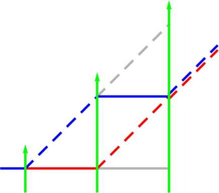
Figure 1: Recoil diagram for the MZAI. Atoms in the ground and excited states are shown by solid and dashed lines, respectively.

If the mirror pulse (second Raman pulse) is a resonant $\pi-$pulse, then the atoms change their momenta and internal states with probability 1. In this case, the diagram has only two branches, red and blue. Atomic interference is the interference of the amplitudes of an atom in an excited state $e$, which arise when an atom moves along these branches. In this case, the contrast of the interference pattern is equal to $1$. If the second pulse is not ideal, then the atoms do not change their state with a small amplitude (see the gray lines in the recoil diagram). Obviously, this only leads to a decrease in contrast and does not affect the phase of the MZAI.

The situation changes for SLMT, when in addition to the three main Raman pulses there are four sets of auxiliary $\pi-$pulses, after the first, before and after the second and before the third main pulses. Consider the simplest case, when each of the sets consists of only one $\pi-$pulse (see Fig. 2).

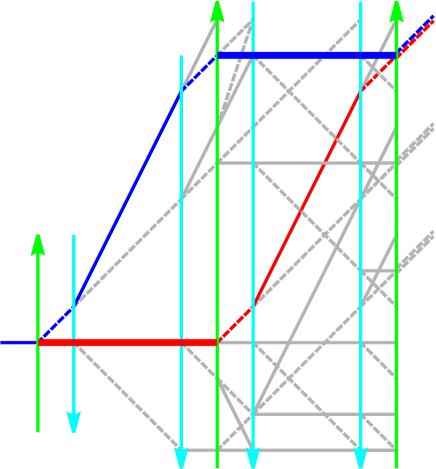
Figure 2: SLMT. Each of the four sets of auxiliary pulses contains one $\pi-$pulse. The main and auxiliary pulses are shown with green and cyan arrows, respectively. Thin, blue or red lines correspond to the resonant branches of the diagram, along which the momentum of the Raman field $\pm\mathbf{\hbar}\mathbf{k}$ is transferred to the atom and the internal state of the atom changes. The thick horizontal lines correspond to the non-resonant branches of the diagram, along which the atoms remain in the ground state $g$, and the momentum of the atom also does not change.

Each of the auxiliary pulses must satisfy the two requirements i10 :

1. It must be a resonant $\pi-$pulse on the resonant branch of the recoil diagram;

2. One has to choose the pulse parameters in such a way that the state of the unexcited atom on the other (nonresonant) branch remains unchanged.

If both requirements are met exactly, then, by successively applying auxiliary pulses $n$ times with alternative wave vectors $\pm\mathbf{k}$, one obtains a beam splitter with momentum transfer

$$\Delta\mathbf{p}=\left(n+1\right)\hbar\mathbf{k},$$ (5)

and the excitation probability of an atom in a uniform gravity field $\mathbf{g}$ oscillates as

$$w = \dfrac{1}{2}\left[1-\cos\left(\alpha+\phi_{g}\right)\right],$$ (6a)

$$\phi_{g} = \left(n+1\right)\mathbf{k}\cdot\mathbf{g}T^{2},$$ (6b)

where the parameter $$\alpha \alpha^{\prime} \alpha^{\prime\prime}$$, like the parameters and below in Eqs. (8, 14), are parts of the AI phase, independent of gravity.

In the Raman-Nath regime (4), when the pulse is so short that the violation of resonance conditions becomes insignificant, one can ignore both the first and the second requirements. In this case, the SLMT is twice as efficient, leading to the momentum transfer

$$\Delta\mathbf{p}=\left(2n+1\right)\hbar\mathbf{k}.$$ (7)

The SLMT in the Raman-Nath approximation was observed in Ref. i14 for the one-photon transition. We are not aware of Raman beam splitters operating in the Raman-Nath regime (4).

Condition 2 can be satisfied in the Bragg regime (1). In this case, if the Raman pulse is resonant to a transition along one of the branches, then it is not resonant for the other branch, and with accuracy (1) one can assume that the state of the atom remains unperturbed along the other branch. If the pulse is not perfect, and the parameter $\varepsilon$ is not small enough, then the pulse ceases to be a mirror, splits the states of the atom, and parasitic gray trajectories appear (see Figs. 1 and 2). One sees that, unlike the usual MZAI, in the MZAI with one auxiliary $\pi-$pulse, parasitic trajectories lead to the appearance of parasitic interference ports, due to which a small addition to the signal (6) arises, which oscillates like

$$\Delta w=\beta\cos\left(\alpha^{\prime}+\mathbf{k}\cdot\mathbf{g}T^{2}\right).$$ (8)

It should be emphasized that for precision measurements it is not enough that this correction be small, it is necessary that the amplitude of this correction be less than the accuracy of the MZAI phase measurement $\phi_{\mathrm{err}}$

$$\left|\beta\right|<\phi_{\mathrm{err}}.$$ (9)

Only in this case does SLMT lead to progress in improving the accuracy of precision measurements. The error in the differential measurements of the MZAIs phases was i15

$$\phi_{\mathrm{err}}\approx 2zc10^{-5}\text{rad.}$$ (10)

One sees from Fig. 2 that parasitic ports are spatially separated from the main port by a distance

$$\Delta z=v_{r}T,$$ (11)

where $v_{r}=\left|\mathbf{v}_{r}\right|$ and

$$\mathbf{v}_{r}=\dfrac{\hbar\mathbf{k}}{M}$$ (12)

is the recoil velocity. Under the experimental conditions i10 , $k=1.61\times 10^{7}$ m^-1, $M=87$ a.u., and $T=1.04$ s, the ports are separated from each other by a distance of $\Delta z=1.2$ cm. If, despite thermal expansion, the size of the atomic cloud, as well as the size of the detector, is less than $\Delta z$, then one can exclude the influence of parasitic ports.

The situation changes if several $\pi-$pulses are used in each auxiliary set, $n>1$. The case $n=2$ is shown in Fig. 3. One sees that the distance between the main and parasitic ports decreases to the value

$$\Delta z=v_{r}d,$$ (13)

where $d$ is the delay between adjacent auxiliary pulses. At $d=200~{}\mu$s i16 $\Delta z\approx 2.4~{}\mu.$ One may encounter technological difficulties in creating detectors and atomic clouds of such a small size. Otherwise, the ports overlap and parasitic signals occur. For example, a port caused by the interference of the blue-orange and red-purple branches (see Fig. 3) results in a parasitic signal

$$\Delta w=\beta\cos\left(\alpha^{\prime\prime}+2\mathbf{k}\cdot\mathbf{g}T^{2}\right).$$ (14)

With a larger number of auxiliary pulses, the role of parasitic terms can increase even more. Thus, for precision interferometry, it is necessary to use such beam splitters that satisfy requirements 1 and 2 with the greatest accuracy. To satisfy requirement 1, it is enough to adjust the Raman frequency detuning of a given pulse to the frequency of the transition between the atomic momentum states before and after the action of the field, while for requirement 2, we propose in this paper to use Rabi oscillations i17 instead of the Bragg regime i10 . For the nonresonant branch, one can find such a pulse duration

$$\tau\sim\omega_{k}^{-1},$$ (15)

at which the probability of state splitting on this branch will be exactly 0. Below we find this duration for a rectangular Raman pulse and calculate the phase of the MZAI.

Since the pulse on the resonant branch must have an area $\pi$, the effective Rabi frequency $\Omega$ of a two-quantum transition between atomic states for auxiliary pulses may not coincide with the Rabi frequency for the main pulses. This, to a certain extent, is a technological challenge, the implementation of SLMT with sets of pulses having different intensities and durations. To circumvent this difficulty, we propose to use composite pulses i18 , and we consider only non-contiguous composite pulses (NCPs) i18.1 . These pulses, as in Ref. i10 , must be in resonance with atomic transitions $\left|\mathbf{p}+m\hbar\mathbf{k}\right\rangle\leftrightarrow\left|\mathbf{p}+\left(m-1\right)\hbar\mathbf{k}\right\rangle$, where $m>1$ is an integer, their frequencies differ from the frequencies of the main pulses, resonant to transitions $\left|\mathbf{p}\right\rangle\longleftrightarrow\left|\mathbf{p}+\mathbf{\hbar k}\right\rangle$, and they also differ from each other. However, the Rabi frequency for all pulses is the same, and the sum of the pulse durations in a given NCP should be equal to $2\tau$, where $\tau$ is the duration of the first and third main $\dfrac{\pi}{2}-$ pulses. If the composite pulse consists of two rectangular pulses, then each of them can have a duration $\tau$.

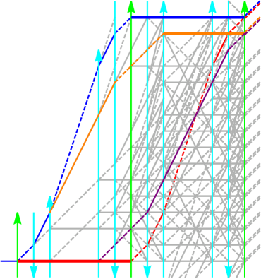
Figure 3: Same as in Fig. 2, but for $n=2$, when each set of auxiliary pulses contains two $\pi-$pulses with opposite effective wave vectors. One included only color output ports in consideration.

Below we consider the NCP, consisting of three rectangular pulses. If the durations of the first and third pulses coincide, then obviously the duration of each of the rectangular pulses can vary in the range $\left[0,\tau\right]$. Under the action of a composite pulse, the atom performs Rabi oscillations during each of the pulses, and nutation of atomic coherence takes place in the time between rectangular pulses. Below we find such delay between pulses

$$\tau_{b}\sim\omega_{k}^{-1},$$ (16)

under which, owing to a combination of nutation and Rabi oscillations, requirement 2 is satisfied precisely.

I.2 Recoil phase

It is well known that atomic interference is caused by the quantization of the motion of the atomic center-of-mass. When the incident atomic momentum state $\left|\mathbf{p}\right\rangle$ splits into two states $\left|\mathbf{p}\right\rangle$ and $\left|\mathbf{p}+\mathbf{\hbar k}\right\rangle$ after passing through the beam splitter, the coherence between these states evolves as

$$\rho\left(\mathbf{p}+\hbar\mathbf{k},\mathbf{p},t\right)\propto\exp\left(-i\omega_{\mathbf{p}+\hbar\mathbf{k},\mathbf{p}}t\right),$$ (17)

where the frequency of transition between states

$$\omega_{\mathbf{p}+\hbar\mathbf{k},\mathbf{p}} = \dfrac{1}{2M\hbar}\left[\left(\mathbf{p}+\hbar\mathbf{k}\right)^{2}-\mathbf{p}^{2}\right]=\omega_{D}+\omega_{k},$$ (18a)

$$\omega_{D} = \mathbf{k}\cdot\dfrac{\mathbf{p}}{M},$$ (18b)

along with the Doppler frequency shift $$\omega_{D} t\sim T$$, contains a quantum term, the recoil frequency (2). If one can expect that the AI phase contains Doppler and quantum terms

$$\phi_{D} \sim \omega_{D}T,$$ (19a)

$$\phi_{q} \sim \omega_{k}T.$$ (19b)

Despite this, the phase of the well-known and widely used MZAI does not contain any quantum term in a uniform gravity field [see Eq. (6b) for $$n=0$$]. The reason is that, although quantum corrections affect changes in the atom’s coordinates at the moments of interaction with the second and third beam splitters, the corresponding quantum terms compensate each other in a uniform gravity field (see Appendix A in Ref. i19 ). We would like to emphasize that the derivation of the expression for the AI phase is purely quantum (see examples of this derivation in Refs. i20 ; i6 ; i19 ), but the result of these derivations, Eq. (6b), is purely classical. The absence of a quantum phase (19b) allows one to be in doubt that the MZAI is caused by the matter waves interference (a sentiment held by the present author). Examples of the derivation of the expression for the phase without using the atomic center-of-mass motion quantization can be found in preprint i20.1 .

The quantum contribution arises in the rotating reference frame i21 , or in the non-uniform gravity field in the presence of the gravity-gradient tensor i22 ; i23 , or in the presence of the gravity-gradient tensor of the second order i24 , or in a strongly inhomogeneous source mass field i24 . The quantum term in the gravity-gradient field of the source mass was observed in i25 using the LMT method. In all these cases, the magnitude of the quantum terms is small compared to the phase $\phi_{q}$ in Eq. (19b). We predict here that the situation may change dramatically in the presence of auxiliary pulses. If the ultimate goal is not to create a high-precision gravimeter, but, as in i25 , to observe the quantum term, and the timing of these pulses is comparable to the interrogation time $T$, then the quantum term turns out to be large and grows as $n/\ln n$ with increasing momentum transfer.

It should be noted, however, that the quantum term does not arise if, as in the experiments in i10 ; i14 ; i16 , the auxiliary pulses are equidistant in time. With nonequidistant timing, the quantum term does not depend on the shape and duration of the pulse, it is the same for the rectangular pulses considered here, as well as in the Bragg regime i10 . However, for SLMT in the Raman-Nath approximation (4), for the both Raman beam splitters and atomic clocks i14 , the quantum term must be recalculated.

Figure 4: Atomic level diagram

I.3 The article structure

In this article, we use the Schrödinger equation in momentum space, in contrast to the same approach in preprints i19 ; i26 , here we take into account the motion of the atom during the time of interaction with the pulse.

The overall plan of the paper is as follows. In the next section, we use the solutions of the Schrödinger equation for the interaction of an atom with a rectangular pulse to determine the parameters of the NCPs, consisting of one, two and three rectangular pulses. In Sec. III we calculate the MZAI phase. In Sec. IV we consider 2 types of quantum parts of MZAI phases. In Sec. V, an expression for the gravity part of the MZAI phase is obtained. We calculate the part of the gravity phase, independent of the duration of the main and auxiliary pulses, and corrections linear in these durations.

II Main relations.

Let us consider the interaction of a three-level atom with the pulse of the field of two traveling waves resonant to adjacent atomic transitions

$$\mathbf{E}\left(\mathbf{x},t\right)=\left\{\mathbf{E}_{1}\exp\left[i\left(\mathbf{q}_{1}\cdot\mathbf{x}-\omega_{1}t-\phi_{1}\left(t\right)\right)\right]+\mathbf{E}_{2}\exp\left[i\left(\mathbf{q}_{2}\cdot\mathbf{x}-\omega_{2}t-\phi_{2}\left(t\right)\right)\right]\right\}f\left(t\right)+c.c,$$ (20)

where $E_{i},$ $\mathbf{q}_{i},\omega_{i}$ and $\phi_{i}\left(t\right)$ are the amplitudes, wave vectors, frequencies and phases of the waves, respectively, and $f\left(t\right)$ is the shape of the pulse acting at the moment $T$ and having a duration $\tau$. We assume that the two atomic states $\left|g\right\rangle$ and $\left|e\right\rangle$ are sublevels of the hyperfine structure of the ground-state manifold of the atom, while the third state $\left|o\right\rangle$ is a sublevel of the excited-state manifold; the fields $\mathbf{E}_{1}$and $\mathbf{E}_{2}$ are resonant to the atomic transitions $g\rightarrow o$ and $e\rightarrow o$ (see Fig. 4). The location of the sublevels $\left|g\right\rangle$ and $\left|e\right\rangle$ on the atomic energy diagram is not important. However, we consider sublevels $\left|g\right\rangle$ and $\left|e\right\rangle$ to be ground and excited.

The Hamiltonian of the interaction of an atom with a field is

$$H=\dfrac{p^{2}}{2M}-M\mathbf{g\cdot x}+\dfrac{\hbar}{2}\left\{\Omega_{1}\exp\left[i\left(\mathbf{q}_{1}\cdot\mathbf{x}-\Delta_{1}t-\phi_{1}\left(t\right)\right)\right]\left|o\right\rangle\left\langle g\right|+\Omega_{2}\exp\left[i\left(\mathbf{q}_{2}\cdot\mathbf{x}-\Delta_{2}t-\phi_{2}\left(t\right)\right)\right]\left|o\right\rangle\left\langle e\right|+H.c.\right\}f\left(t\right),$$ (21)

where $\mathbf{p}$ is the momentum of the atom; and $\mathbf{g}$ is the gravity field;

$$\Omega_{1} \equiv -2\dfrac{\mathbf{d}_{og}\mathbf{\cdot E}_{1}}{\hbar},$$ (22a)

$$\Omega_{2} \equiv -2\dfrac{\mathbf{d}_{oe}\mathbf{\cdot E}_{2}}{\hbar}$$ (22b)

are the Rabi frequencies of atomic transitions, with $$\mathbf{d}$$ the dipole moment operator; and

$$\Delta_{1} = \omega_{1}-\omega_{og},$$ (23a)

$$\Delta_{2} = \omega_{2}-\omega_{oe}$$ (23b)

are frequency detunings of the fields. The amplitudes of atomic levels evolve as

$$i\partial_{t}\tilde{a}\left(e,\mathbf{p},t\right) = \left(\dfrac{p^{2}}{2M\hbar}-iM\mathbf{g\cdot}\partial_{\mathbf{p}}\right)\tilde{a}\left(e,\mathbf{p},t\right)+\dfrac{\Omega_{2}^{\ast}}{2}\exp\left[i\left(\Delta_{2}t+\phi_{2}\left(t\right)\right)\right]f\left(t\right)\tilde{a}\left(o,\mathbf{p}+\hbar\mathbf{q}_{2},t\right),$$ (24a)

$$i\partial_{t}\tilde{a}\left(g,\mathbf{p},t\right) = \left(\dfrac{p^{2}}{2M\hbar}-iM\mathbf{g\cdot}\partial_{\mathbf{p}}\right)\tilde{a}\left(g,\mathbf{p},t\right)+\dfrac{\Omega_{1}^{\ast}}{2}\exp\left[i\left(\Delta_{1}t+\phi_{1}\left(t\right)\right)\right]f\left(t\right)\tilde{a}\left(o,\mathbf{p}+\hbar\mathbf{q}_{1},t\right),$$ (24b)

$$i\partial_{t}\tilde{a}\left(o,\mathbf{p},t\right) = \left(\dfrac{p^{2}}{2M\hbar}-iM\mathbf{g\cdot}\partial_{\mathbf{p}}\right)\tilde{a}\left(o,\mathbf{p},t\right)+\dfrac{\Omega_{1}}{2}\exp\left[-i\left(\Delta_{1}t+\phi_{1}\left(t\right)\right)\right]f\left(t\right)\tilde{a}\left(g,\mathbf{p}-\hbar\mathbf{q}_{1},t\right)$$ (24c)

$$+\dfrac{\Omega_{2}}{2}\exp\left[-i\left(\Delta_{2}t+\phi_{2}\left(t\right)\right)\right]f\left(t\right)\tilde{a}\left(e,\mathbf{p}-\hbar\mathbf{q}_{2},t\right).$$

One assumes that the frequency detuning is large enough

$$\Delta_{1} \approx \Delta_{2}\approx\Delta,$$ (25a)

$$\left|\Delta\right| \gg \max\left\{\left|\tilde{\delta}\right|,\tau_{f}^{-1},\left|\dot{\phi}_{i}\right|,\left|\mathbf{q}_{i}\cdot\mathbf{g}\right|T,\left|\omega_{D}\right|,\omega_{k}\right\},$$ (25b)

where

$$\tilde{\delta}=\Delta_{1}-\Delta_{2}$$ (26)

is a Raman detuning, and $\tau_{f}$ is the duration of the forward and backward fronts of the pulse. At this assumption one finds the expression for the level $\left|o\right\rangle$ amplitude i26.1

$$\tilde{a}\left(o,\mathbf{p},t\right)=\dfrac{f\left(t\right)}{2\Delta}\left\{\Omega_{1}\exp\left[-i\left(\Delta_{1}t+\phi_{1}\left(t\right)\right)\right]\tilde{a}\left(g,\mathbf{p}-\hbar\mathbf{q}_{1},t\right)+\Omega_{2}\exp\left[-i\left(\Delta_{2}t+\phi_{2}\left(t\right)\right)\right]\tilde{a}\left(e,\mathbf{p}-\hbar\mathbf{q}_{2},t\right)\right\}.$$ (27)

Then for the amplitudes of the ground state sublevels one gets

$$i\partial_{t}\tilde{a}\left(e,\mathbf{p},t\right) = \left(\dfrac{p^{2}}{2M\hbar}-iM\mathbf{g\cdot}\partial_{\mathbf{p}}+\dfrac{\left|\Omega_{2}\right|^{2}}{4\Delta}\right)\tilde{a}\left(e,\mathbf{p},t\right)+\dfrac{\Omega}{2}\exp\left[-i\left(\tilde{\delta}t+\phi\left(t\right)\right)\right]f^{2}\left(t\right)\tilde{a}\left(g,\mathbf{p}-\hbar\mathbf{k},t\right),$$ (28a)

$$i\partial_{t}\tilde{a}\left(g,\mathbf{p},t\right) = \left(\dfrac{p^{2}}{2M\hbar}-iM\mathbf{g\cdot}\partial_{\mathbf{p}}+\dfrac{\left|\Omega_{1}\right|^{2}}{4\Delta}\right)\tilde{a}\left(g,\mathbf{p},t\right)+\dfrac{\Omega^{\ast}}{2}\exp\left[i\left(\tilde{\delta}t+\phi\left(t\right)\right)\right]f^{2}\left(t\right)\tilde{a}\left(e,\mathbf{p}+\hbar\mathbf{k},t\right),$$ (28b)

where

$$\mathbf{k} = \mathbf{q}_{1}-\mathbf{q}_{2},$$ (29a)

$$\Omega = \dfrac{\Omega_{1}\Omega_{2}^{\ast}}{2\Delta},$$ (29b)

$$\phi\left(t\right) = \phi_{1}\left(t\right)-\phi_{2}\left(t\right)$$ (29c)

are the effective wave vector, the Rabi frequency, and the phase of the Raman beam splitter, respectively. Eliminating the ac-Stark shift by a transformation to a rotating interaction picture, i.e. by introducing the amplitudes

$$\left(\begin{array}[]{c}\tilde{a}\left(e,\mathbf{p},t\right)\\ \tilde{a}\left(g,\mathbf{p},t\right)\end{array}\right)=\exp\left[-\dfrac{i}{4\Delta}\int^{t}dt^{\prime}\left(\begin{array}[]{c}\left|\Omega_{2}\right|^{2}\\ \left|\Omega_{1}\right|^{2}\end{array}\right)f^{2}\left(t^{\prime}\right)\right]\left(\begin{array}[]{c}a\left(e,\mathbf{p},t\right)\\ a\left(g,\mathbf{p},t\right)\end{array}\right)$$ (30)

one obtains

$$i\left(\partial_{t}+M\mathbf{g\cdot}\partial_{\mathbf{p}}+i\dfrac{p^{2}}{2M\hbar}\right)a\left(e,\mathbf{p},t\right) = \dfrac{\Omega}{2}f^{2}\left(t\right)\exp\left[-i\delta t-i\phi\left(t\right)\right]a\left(g,\mathbf{p}-\hbar\mathbf{k},t\right),$$ (31a)

$$i\left(\partial_{t}+M\mathbf{g\cdot}\partial_{\mathbf{p}}+i\dfrac{p^{2}}{2M\hbar}\right)a\left(g,\mathbf{p},t\right) = \dfrac{\Omega^{\ast}}{2}f^{2}\left(t\right)\exp\left(i\delta t+i\phi\left(t\right)\right)a\left(e,\mathbf{p}+\hbar\mathbf{k},t\right),$$ (31b)

where

$$\delta = \tilde{\delta}-\delta_{S},$$ (32a)

$$\delta_{S} = \dfrac{\left|\Omega_{2}\right|^{2}-\left|\Omega_{1}\right|^{2}}{4\Delta}$$ (32b)

is the ac-Stark shift of the Raman line. The presence of an ac-Stark shift would significantly complicate the present study. We will assume that this shift is absent. Experimental methods for eliminating the ac-Stark shift were developed in Refs. i26.3 ; i26.4 . If, for example, the Raman pulse has an area $$\dfrac{\pi}{2} \delta_{S}=0$$, then from the equation and Eq. (29b) one has

$$\left|\Omega_{1}\right|=\sqrt{\dfrac{\pi\left|\Delta\right|}{\tau}}.$$ (33)

At typical values of $\Delta=2\pi\times 10$GHz  and $\tau=30~{}\mu$s, the parameter

$$\left|\Omega_{1}\right|/\Delta\approx 7\times 10^{-4}$$ (34)

is small enough to neglect the ac-Stark splitting of optical transitions $e\rightarrow o$ and $g\rightarrow o$i27 .

In an accelerated frame

$$\mathbf{p}=\mathbf{P}+M\mathbf{g}t,$$ (35)

using the atom’s initial momentum $\mathbf{P}$ as the independent variable, one gets

$$i\left(\dfrac{d}{dt}+i\dfrac{\left(\mathbf{P}+M\mathbf{g}t\right)^{2}}{2M\hbar}\right)a\left(e,\mathbf{P},t\right) = \dfrac{\Omega}{2}f^{2}\left(t\right)\exp\left[-i\delta t-i\phi\left(t\right)\right]a\left(g,\mathbf{P}-\hbar\mathbf{k},t\right),$$ (36a)

$$i\left(\dfrac{d}{dt}+i\dfrac{\left(\mathbf{P}+M\mathbf{g}t\right)^{2}}{2M\hbar}\right)a\left(g,\mathbf{P},t\right) = \dfrac{\Omega^{\ast}}{2}f^{2}\left(t\right)\exp\left[i\delta t+i\phi\left(t\right)\right]a\left(e,\mathbf{P}+\hbar\mathbf{k},t\right).$$ (36b)

Then one finds that in the interaction representation

$$a\left(n,\mathbf{P},t\right)=\exp\left[-i\int_{0}^{t}dt^{\prime}\dfrac{\left(\mathbf{P}+M\mathbf{g}t^{\prime}\right)^{2}}{2M\hbar}\right]c\left(n,\mathbf{P},t\right)$$ (37)

state vector

$$\underline{c}\left(\mathbf{P},t\right)=\left(\begin{array}[]{c}c\left(e,\mathbf{P}+\dfrac{\hbar\mathbf{k}}{2},t\right)\\ c\left(g,\mathbf{P}-\dfrac{\hbar\mathbf{k}}{2},t\right)\end{array}\right)$$ (38)

evolves as

$$i\underline{\dot{c}}=\dfrac{f^{2}\left(t\right)}{2}\left(\begin{array}[]{cc}0&\Omega\exp\left\{-i\left[\delta t+\phi\left(t\right)-\mathbf{k\cdot}\dfrac{\mathbf{P}}{M}t-\dfrac{1}{2}\mathbf{k\cdot g}t^{2}\right]\right\}\\ \Omega^{\ast}\exp\left\{i\left[\delta t+\phi\left(t\right)-\mathbf{k\cdot}\dfrac{\mathbf{P}}{M}t-\dfrac{1}{2}\mathbf{k\cdot g}t^{2}\right]\right\}&0\end{array}\right)\underline{c}.$$ (39)

One sees that in the accelerated frame the amplitude of the atomic state remains unchanged outside the field pulse

$$\underline{c}\left(\mathbf{P},t\right)=\text{const at }t<T\text{ or }t>T+\tau$$ (40)

If one chirps the field frequency linearly, i.e., if

$$\phi\left(t\right)=\phi+\alpha t^{2}/2,$$ (41)

and if the chirping rate $\alpha$ is close to $\mathbf{k}\cdot\mathbf{g},$

$$\left|\alpha-\mathbf{k\cdot g}\right|\tau^{2}\ll 1,$$ (42)

then, considering Eq. (39) when

$$t=T+\varepsilon,$$ (43)

where

$$\varepsilon\sim\tau\ll T,$$ (44)

and neglecting terms quadratic in $\varepsilon$ in the phase factors in Eq. (39), one arrives at the well-known equation for the amplitudes of a two-level atom interacting with the pulse of the field of arbitrary shape with constant frequency and phase

$$i\dfrac{d\underline{c}}{d\varepsilon}=\dfrac{f^{2}\left(T+\varepsilon\right)}{2}\left(\begin{array}[]{cc}0&\Omega\exp\left\{-i\left[\nu\varepsilon+\phi\left(\mathbf{P}\right)\right]\right\}\\ \Omega^{\ast}\exp\left\{i\left[\nu\varepsilon+\phi\left(\mathbf{P}\right)\right]\right\}&0\end{array}\right)\underline{c},$$ (45)

where

$$\nu \equiv \delta\left(\mathbf{P}\right)=\nu^{\left(0\right)}+\nu^{\left(1\right)},$$ (46a)

$$\nu^{\left(0\right)} \equiv \delta^{\left(0\right)}\left(\mathbf{P}\right)=\delta-\mathbf{k\cdot}\dfrac{\mathbf{P}}{M},$$ (46b)

$$\nu^{\left(1\right)} = -\left(\mathbf{k\cdot g}-\alpha\right)T,$$ (46c)

$$\phi\left(\mathbf{P}\right) = \phi+\nu^{\left(0\right)}T-\dfrac{1}{2}\left(\mathbf{k\cdot g}-\alpha\right)T^{2}.$$ (46d)

After unitary transformation

$$\underline{c}=\underline{U}_{\phi}\underline{\tilde{b}},$$ (47)

where the matrix $U_{\phi}$ is given by

$$\underline{U}_{\phi}=\left(\begin{array}[]{cc}\exp\left[-\dfrac{i}{2}\phi\left(\mathbf{P}\right)\right]&0\\ 0&\exp\left[\dfrac{i}{2}\phi\left(\mathbf{P}\right)\right]\end{array}\right),$$ (48)

one arrives at the phase-independent equation

$$i\dfrac{d\underline{\tilde{b}}}{d\varepsilon}=\dfrac{f^{2}\left(T+\varepsilon\right)}{2}\left(\begin{array}[]{cc}0&\Omega\exp\left(-i\nu\varepsilon\right)\\ \Omega^{\ast}\exp\left(i\nu\varepsilon\right)&0\end{array}\right)\underline{\tilde{b}}.$$ (49)

In the AI phase, the factor $\exp\left[\pm\dfrac{i}{2}\phi\left(\mathbf{P}\right)\right]$ will be responsible for the Doppler and quantum phases (19), for the gravity phase (6b), as well as for the Ramsey phase

$$\phi_{R}\sim\delta T.$$ (50)

One might conclude that the results to be obtained below for the quantum, gravity and Ramsey phases are independent of the pulse shape $f\left(t\right)$ and do not change from the Raman-Nath regime (4) to the Bragg regime (1).

Consider now a NCP consisting of $\ell$ time-separated rectangular pulses

$$f\left(T+\varepsilon\right)=\left\{\begin{array}[]{l}1\text{\quad for }\varepsilon\in\mathop{\displaystyle\bigcup}\limits_{m=1}^{\ell}\left[\tau_{0,m},\tau_{0,m}+\tau_{m}\right]\\ 0\text{\quad in other cases,}\end{array}\right.$$ (51)

where one turns on a pulse of duration $\tau_{m}$ at time $T+\tau_{0,m}$, so that

$$\tau_{0,m}=\mathop{\displaystyle\sum}_{m^{\prime}=1}^{m-1}\left(\tau_{m^{\prime}}+\tau_{bm^{\prime}}\right),$$ (52)

where $\tau_{bm}$ is the delay time between adjacent pulses $m$ and $m+1$. After the next unitary transformation

$$\underline{\tilde{b}} = \underline{U}_{\delta}\underline{b},$$ (53a)

$$U_{\delta} = \left(\begin{array}[]{cc}\exp\left(-\dfrac{i}{2}\nu\varepsilon\right)&0\\ 0&\exp\left(\dfrac{i}{2}\nu\varepsilon\right)\end{array}\right)$$ (53d)

one finds

$$i\dfrac{d\underline{b}}{d\varepsilon} = \underline{h}\underline{b},$$ (54a)

$$\underline{h} = \dfrac{1}{2}\left(\begin{array}[]{cc}-\nu&\Omega\\ \Omega^{\ast}&+\nu\end{array}\right)$$ (54d)

The solution of this equation is well known. One can achieve it using composite rotation matrices. Alternatively, one can represent the $$h-$$matrix as

$$\underline{h}=\mathbf{h\cdot}\underline{\mathbf{\sigma}},$$

where

$$\mathbf{h=}\dfrac{1}{2}\left\{\mathop{\mathrm{R}e}\Omega,-\mathop{\mathrm{I}m}\Omega,-\nu\right\}$$

and $\underline{\mathbf{\sigma}}=\left\{\underline{\sigma}_{1},\underline{\sigma}_{2},\underline{\sigma}_{3}\right\},$ with $\underline{\sigma}_{i}$ the Pauli matrix, and for the $s-$matrix $\underline{\sigma}=epx\left(-i\underline{h}t\right)$ use the expression i26.2

$$\underline{f}\left(\mathbf{h\cdot\underline{\sigma}}\right)=\dfrac{1}{2}\left\{f\left(h\right)+f\left(-h\right)+\dfrac{\mathbf{h\cdot\underline{\sigma}}}{h}\left[f\left(h\right)-f\left(-h\right)\right]\right\}.$$ (55)

Immediately after the action of the pulse $m$, the wave function of the atom is

$$\underline{b}\left(T+\tau_{0,m}+\tau_{m}\right) = \underline{\sigma}\left(\tau_{m}\right)\underline{b}\left(T+\tau_{0,m}\right),$$ (56a)

$$\underline{\sigma}\left(\tau\right) = \left(\begin{array}[]{cc}s_{d}\left(\tau\right)&-is_{a}\left(\tau\right)\\ -is_{a}^{\ast}\left(\tau\right)&s_{d}^{\ast}\left(\tau\right)\end{array}\right),$$ (56d)

$$s_{d}\left(\tau\right) = \cos\dfrac{\Omega_{r}\tau}{2}+i\dfrac{\nu}{\Omega_{r}}\sin\dfrac{\Omega_{r}\tau}{2},$$ (56e)

$$s_{a}\left(\tau\right) = \dfrac{\Omega}{\Omega_{r}}\sin\dfrac{\Omega_{r}\tau}{2},$$ (56f)

$$\Omega_{r} = \sqrt{\left|\Omega\right|^{2}+\nu^{2}}.$$ (56g)

Hence, for $$\Omega=0 \tau_{bm} s-$$, corresponding to the time between pulses , the matrix is

$$\underline{s}_{bm}=\left(\begin{array}[]{cc}\exp\left(\dfrac{i}{2}\nu\tau_{bm}\right)&0\\ 0&\exp\left(-\dfrac{i}{2}\nu\tau_{bm}\right)\end{array}\right).$$ (57)

The numbering of auxiliary NCPs $\left\{\zeta,\beta\right\}$ will be introduced below in Sec. III, where one verifies that either the pulse duration at $\ell=1$ or the distance between pulses at $\ell>1$ depends on the Raman detuning $\nu$ on the nonresonant branch of the recoil diagram so that the total time of action of this NCP is a function of four parameters $\left\{\nu,\zeta,\beta,\ell\right\}$, for which one has

$$\tau\left(\nu,\zeta,\beta,\ell\right)=\tau_{\ell}+\mathop{\displaystyle\sum}_{m=1}^{\ell-1}\left(\tau_{m}+\tau_{bm}\right),$$ (58)

For the $s-$matrix one has

$$\underline{s}=\underline{\sigma}\left(\tau_{\ell}\right)\underline{s}_{b\left(\ell-1\right)}\underline{\sigma}\left(\tau_{\ell-1}\right)\cdots\underline{s}_{b1}\underline{\sigma}\left(\tau_{1}\right).$$ (59)

Now, returning to the state vector (38) and to the lab frame,

$$\mathbf{P} = \mathbf{p}_{+,T+\tau\left(\nu,\zeta,\beta,\ell\right)},$$ (60a)

$$\mathbf{p}_{t} \equiv \mathbf{p}-M\mathbf{g}t,$$ (60b)

one arrives at the next result

$$c\left(e,\mathbf{p}_{+},T+\tau\left(\nu,\zeta,\beta,\ell\right)\right)=S_{ee}\left(\mathbf{p}_{+,T+\tau\left(\nu,\zeta,\beta,\ell\right)}-\dfrac{\hbar\mathbf{k}}{2}\right)c\left(e,\mathbf{p}_{-},T\right)+S_{eg}\left(\mathbf{p}_{+,T+\tau\left(\nu,\zeta,\beta,\ell\right)}-\dfrac{\hbar\mathbf{k}}{2}\right)c\left(g,\mathbf{p}_{-}-\hbar\mathbf{k},T\right),$$ (61a)

$$c\left(g,\mathbf{p}_{+},T+\tau\left(\nu,\zeta,\beta,\ell\right)\right)=S_{ge}\left(\mathbf{p}_{+,T+\tau\left(\nu,\zeta,\beta,\ell\right)}+\dfrac{\hbar\mathbf{k}}{2}\right)c\left(e,\mathbf{p}_{-}+\hbar\mathbf{k},T\right)+S_{gg}\left(\mathbf{p}_{+,T+\tau\left(\nu,\zeta,\beta,\ell\right)}+\dfrac{\hbar\mathbf{k}}{2}\right)c\left(g,\mathbf{p}_{-},T\right),$$ (61b)

where

$$S\left(\mathbf{P}\right) = \left(\begin{array}[]{cc}\hat{s}_{ee}&\exp\left[-i\phi\left(\mathbf{P}\right)\right]\hat{s}_{eg}\\ \exp\left[i\phi\left(\mathbf{P}\right)\right]\hat{s}_{ge}&\hat{s}_{gg}\end{array}\right),$$ (62c)

$$\underline{\hat{s}} = \left(\begin{array}[]{cc}\exp\left[-\dfrac{i}{2}\nu\tau\left(\nu,\zeta,\beta,\ell\right)\right]s_{ee}&\exp\left[-\dfrac{i}{2}\nu\tau\left(\nu,\zeta,\beta,\ell\right)\right]s_{eg}\\ \exp\left[\dfrac{i}{2}\nu\tau\left(\nu,\zeta,\beta,\ell\right)\right]s_{ge}&\exp\left[\dfrac{i}{2}\nu\tau\left(\nu,\zeta,\beta,\ell\right)\right]s_{gg}\end{array}\right).$$ (62f)

where $$s_{\alpha\beta} s-$$ is a matrix element of the matrix (59).

meaning1The momentum of the atom changes due to the transfer of the momentum of the photon $\pm\hbar\mathbf{k}$ and under the action of gravitation $\mathbf{g}$. The change in the momentum of the atom under the action of a uniform gravitational field does not depend on the initial value of the momentum [see Eq. (60b)] and therefore does not depend on the momentum of the photon transferred to the atom. This allows one to represent the momenta of an atom as

$$\mathbf{p}_{\pm}=\mathbf{p}_{\pm}^{\prime}+\mathfrak{N\hbar}\mathbf{k},$$ (63)

where $\mathfrak{N}$ is the total number of photon momenta transferred to the atom at a given point in the recoil diagram. Below we omit the prime in the expressions for momenta. If the effective wave vector of a given NCP is equal to $\pm\mathbf{k}$, then, keeping in mind the redefinition (63), one obtains, instead of Eqs. (61),

$$c\left(e,\mathbf{p}_{+}+\mathfrak{N}\hbar\mathbf{k},T+\tau\left(\nu,\zeta,\beta,\ell\right)\right) = S_{ee}\left(\mathbf{p}_{+,T+\tau\left(\nu,\zeta,\beta,\ell\right)}+\left(2\mathfrak{N}\mp 1\right)\dfrac{\hbar\mathbf{k}}{2}\right)c\left(e,\mathbf{p}_{-}+\mathfrak{N}\hbar\mathbf{k},T\right)$$ (64a)

$$+S_{eg}\left(\mathbf{p}_{+,T+\tau\left(\nu,\zeta,\beta,\ell\right)}+\left(2\mathfrak{N}\mp 1\right)\dfrac{\hbar\mathbf{k}}{2}\right)c\left(g,\mathbf{p}_{-}+\left(\mathfrak{N}\mp 1\right)\hbar\mathbf{k},T\right),$$

$$c\left(g,\mathbf{p}_{+}+\mathfrak{N}\hbar\mathbf{k},T+\tau\left(\nu,\zeta,\beta,\ell\right)\right) = S_{ge}\left(\mathbf{p}_{+,T+\tau\left(\nu,\zeta,\beta,\ell\right)}+\left(2\mathfrak{N}\pm 1\right)\dfrac{\hbar\mathbf{k}}{2}\right)c\left(e,\mathbf{p}_{-}+\left(\mathfrak{N}\pm 1\right)\hbar\mathbf{k},T\right)$$ (64b)

$$+S_{gg}\left(\mathbf{p}_{+,T+\tau\left(\nu,\zeta,\beta,\ell\right)}+\left(2\mathfrak{N}\pm 1\right)\dfrac{\hbar\mathbf{k}}{2}\right)c\left(g,\mathbf{p}_{-}+\mathfrak{N}\hbar\mathbf{k},T\right).$$

meaning1

The independent variable is the momentum of the atom after interaction with the NCP, $\mathbf{p}_{+}$. Then from Eqs. (60) it follows that the momentum of the atom before this interaction is

$$\mathbf{p}_{-}=\mathbf{p}_{+,\tau\left(\nu,\zeta,\beta,\ell\right)}.$$ (65)

meaning 2 One thus takes into account that during the interaction with the NCP, the atom was accelerated, i.e. before interaction with a given NCP having a duration $\tau$, the momentum of the atom $\mathbf{p}_{-}$ was smaller by $M\mathbf{g\tau}$ than the momentum after the interaction $\mathbf{p}_{+}$.meaning 2

If the NCP $\left\{\zeta,\beta\right\}$ follows the NCP $\left\{\zeta^{\prime},\beta^{\prime}\right\}$, then it follows from Eq. (40) that

$$\underline{c}\left(\mathbf{p}_{-}^{\left(\zeta,\beta\right)},T_{\zeta,\beta}\right) = \underline{c}\left(\mathbf{p}_{+}^{\left(\zeta^{\prime},\beta^{\prime}\right)},T_{\zeta^{\prime},\beta^{\prime}}+\tau\left(\nu^{\prime},\zeta^{\prime},\beta^{\prime},\ell^{\prime}\right)\right),$$ (66a)

$$\mathbf{p}_{+}^{\left(\zeta^{\prime},\beta^{\prime}\right)} = \mathbf{p}_{-,T_{\zeta,\beta}-T_{\zeta^{\prime},\beta^{\prime}}-\tau\left(\nu^{\prime},\zeta^{\prime},\beta^{\prime},\ell^{\prime}\right)}^{\left(\zeta,\beta\right)},$$ (66b)

where $$T_{\zeta,\beta} \left\{\zeta,\beta\right\} \mathbf{p}_{\pm}^{\left(\zeta,\beta\right)} \tau\left(\nu^{\prime},\zeta^{\prime},\beta^{\prime},\ell^{\prime}\right) \left\{\zeta^{\prime},\beta^{\prime}\right\} c \mathbf{p}_{+}$$ is the moment of action of the NCP , is the atomic momentum before and after the action of this NCP, and is the duration (58) of the NCP . meaning 3 Equations (66) mean that atomic state stays unchanged between NCPs and only atomic momentum changes owing to gravity. meaning 3 Knowing , one can restore the momenta of atoms before and after the action of all preceding NCPs applying consequently Eqs. (65, 66b) .

We have not been able to construct an NCP that satisfies requirement 2 for an arbitrary $\ell$. We have done this only for the simplest cases $\ell=1,2$ and $3$. Let’s consider these cases separately.

II.1 Case $\ell=1$

In this case, $\underline{s}=$$\sigma$$\left(\tau\right)$, where $\tau$ is the duration of the NCP and $\sigma$$\left(\tau\right)$ is given in Eqs. (56). In Eqs. (46) Raman frequency detuning consists of two terms, $\nu^{\left(0\right)}$ and $\nu^{\left(1\right)}$. The contribution to the $s-$matrix (56d) from the term $\nu^{\left(1\right)}$ can be estimated as

$$\delta\underline{s}=\underline{s}^{\prime}\nu^{\left(1\right)}\sim\left(\mathbf{k}\cdot\mathbf{g}-\alpha\right)T\tau,$$ (67)

where

$$\underline{s}^{\prime}\equiv\partial\underline{s}/\partial\nu,$$ (68)

and we take into account that the characteristic size of the $s-$matrix dependence on $\nu$, is of the order of $\mathbf{\tau}^{-1}$. The parameter $\left(\mathbf{k}\cdot\mathbf{g}-\alpha\right)T\tau$ is responsible for the corrections to the MZAI phase caused by the finite duration of the Raman pulses i29 ; i31 ; i31.1 . We consider this parameter to be small,

$$\delta\phi\sim\left|\mathbf{k}\cdot\mathbf{g}-\alpha\right|T\tau\ll 1,$$ (69)

and calculate the MZAI phase up to a correction linear in $\tau$.

Here and below we reserve the denotations $\nu$ and $\nu_{r}$ for the Raman frequency detuning on the nonresonant and resonant branches of the recoil diagram, respectively. The effective Rabi frequency

$$\left|\Omega\right|=\dfrac{\pi}{\tau}$$ (70)

Let us first consider the nonresonant branch of the recoil diagram. In the zero approximation in $\delta\phi$ we are looking for such a duration $\tau$ of the auxiliary Raman pulse, at which the atom does not change its state with a probability of $100\%$,

$$\left|s_{gg}\right|=1.$$ (71)

From Eq. (56e), the solution to this equation is

$$\Omega_{r}\tau=2j\pi,$$ (72)

where $j$ is an arbitrary positive integer. From Eqs. (70, 72) one finds that

$$\tau=\pi\dfrac{\sqrt{4j^{2}-1}}{\left|\nu^{\left(0\right)}\right|}.$$ (73)

In this case, the $s-$matrix is

$$\underline{\sigma}\left(\tau\right)=\left(-1\right)^{j}I,$$ (74)

where $I$ is the identity matrix. Consider now the amendments (67). Since

$$s_{d}^{\prime} = -\dfrac{\nu\tau}{2\Omega_{r}}\sin\dfrac{\Omega_{r}\tau}{2}+i\left\{\dfrac{1}{\Omega_{r}}\sin\dfrac{\Omega_{r}\tau}{2}+\dfrac{\nu^{2}\tau}{2\Omega_{r}^{2}}\cos\dfrac{\Omega_{r}\tau}{2}-\dfrac{\nu^{2}}{\Omega_{r}^{3}}\sin\dfrac{\Omega_{r}\tau}{2}\right\},$$ (75a)

$$s_{a}^{\prime} = \dfrac{\Omega\nu}{\Omega_{r}}\left(-\dfrac{1}{\Omega_{r}^{2}}\sin\dfrac{\Omega_{r}\tau}{2}+\dfrac{\tau}{2\Omega_{r}}\cos\dfrac{\Omega_{r}\tau}{2}\right).$$ (75b)

Then from Eqs. (70, 72), one gets that, taking into account corrections linear in $$\tau s-$$, the matrix is

$$\underline{s} = \left(\begin{array}[]{cc}\exp\left\{i\left[\eta_{0}^{\left(1\right)}-\eta_{1}^{\left(1\right)}\left(\nu\right)\nu^{\left(1\right)}\right]\right\}&-i\left(-1\right)^{j}\left[\pi\Omega\left(4j^{2}-1\right)/8j^{2}\left|\Omega\right|\nu\right]\nu^{\left(1\right)}\\ -i\left(-1\right)^{j}\left[\pi\Omega^{\ast}\left(4j^{2}-1\right)/8j^{2}\left|\Omega\right|\nu\right]\nu^{\left(1\right)}&\exp\left\{i\left[\eta_{0}^{\left(1\right)}+\eta_{1}^{\left(1\right)}\left(\nu\right)\nu^{\left(1\right)}\right]\right\}\end{array}\right),$$ (76c)

$$\eta_{0}^{\left(1\right)} = j\pi,$$ (76d)

$$\eta_{1}^{\left(1\right)}\left(\nu\right) = -\dfrac{\pi\left(4j^{2}-1\right)^{3/2}}{8j^{2}\left|\nu\right|}.$$ (76e)

One sees that the correction (46c) due to the small but nonzero pulse duration results in small off-diagonal $$s- s-$$matrix elements. This means that even an ideal rectangular pulse leads to a small splitting of the atomic state on the nonresonant branch of the recoil diagram. In the following, we will only take into account the influence of corrections (46c) on the AI phase, and therefore we will neglect the off-diagonal elements of the matrix (76c).

Let us now turn to the resonance branch. Here, the $\pi-$pulse must, with $100\%$ probability, transfer the atom from one internal state to another, while transmitting the momentum $\pm\hbar\mathbf{k}$. However, at $\nu=0,$ from Eqs. (75), derivatives $\left\{s_{d}^{\prime},s_{a}^{\prime}\right\}=\left\{i\dfrac{\tau}{\pi},0\right\},$ so that

$$\underline{s}=\left(\begin{array}[]{cc}i\tau\nu_{r}^{\left(1\right)}/\pi&-i\exp\left(i\arg\Omega\right)\\ -i\exp\left(-i\arg\Omega\right)&-i\tau\nu_{r}^{\left(1\right)}/\pi\end{array}\right).$$ (77)

One sees that the mirror, the resonant $\pi-$pulse, ceases to be ideal owing to the finite duration of the pulse. With a small amplitude linear in this duration, the momentum of the atom and its internal state remain unchanged. The diagonal elements of the $s-$matrix (77) do not affect the phase of the MZAI, and we neglect them below.

II.2 Case $\ell=2$

We have already noted that the disadvantage of a single Raman pulse is that for each new value of the Raman detuning $\nu^{\left(0\right)}$ one must change the pulse duration according to Eq. (73) and then change the Rabi frequency according to Eq. (70). For $\ell>1$ we will consider NCPs, in which the Rabi frequency is the same as that of the main pulses, and for given durations of rectangular pulses $\tau_{m}$ $\left(m=1,\ldots,\ell\right)$, the condition 2 is reached owing to properly chosen time delays between pulses $\tau_{bm},$ $\left(m=1,\ldots,\ell-1\right)$. Here and below, one reserves the denotation $\tau$ only for the duration of the first main $\dfrac{\pi}{2}-$pulse, so for all pulses the magnitude of the Rabi frequency is

$$\left|\Omega\right|=\dfrac{\pi}{2\tau}$$ (78)

II.2.1 Resonant branch, $\mathbf{\nu}_{r}^{\left(\mathbf{0}\right)}\mathbf{=0}$

For the $s-$matrix (57) one obtains

$$\underline{s}_{bm}=I+\dfrac{i}{2}\nu^{\left(1\right)}\tau_{bm}\underline{\sigma}_{3},$$ (79)

where $\sigma$₃ is the Pauli matrix. Then

$$\underline{s} = \underline{\sigma}\left(\mathop{\displaystyle\sum}_{m=1}^{\ell}\tau_{m}\right)+\delta\underline{s}_{b},$$ (80a)

$$\delta\underline{s}_{b} = \dfrac{i}{2}\nu^{\left(1\right)}\mathop{\displaystyle\sum}_{m=1}^{\ell-1}\tau_{bm}\underline{\sigma}\left(\mathop{\displaystyle\sum}_{m^{\prime}=m+1}^{\ell}\tau_{m^{\prime}}\right)\underline{\sigma}_{3}\underline{\sigma}\left(\mathop{\displaystyle\sum}_{m^{\prime}=1}^{m}\tau_{m^{\prime}}\right).$$ (80b)

Here we have used the law of multiplication for $$s-$$matrices,

$$\underline{\sigma}\left(\tau_{m}\right)\underline{\sigma}\left(\tau_{m-1}\right)=\underline{\sigma}\left(\tau_{m}+\tau_{m-1}\right)$$ (81)

In order for the NCP to be a $\pi-$pulse, it is necessary that the sum of durations $\tau_{m}$ be equal to $2\tau$,

$$\mathop{\displaystyle\sum}_{m=1}^{\ell}\tau_{m}=2\tau.$$ (82)

Then, after the change $\tau\rightarrow 2\tau$ in Eq. (77), one obtains

$$\underline{\sigma}\left(2\tau\right)=\left(\begin{array}[]{cc}2i\tau\nu_{r}^{\left(1\right)}/\pi&-i\exp\left(i\arg\Omega\right)\\ -i\exp\left(-i\arg\Omega\right)&-2i\tau\nu_{r}^{\left(1\right)}/\pi\end{array}\right).$$ (83)

For $\ell=2$ we have considered only the symmetric case, when two rectangular pulses have the same duration

$$\tau_{1}=\tau_{2}=\tau,$$ (84)

when $\delta\underline{s}_{b}=\dfrac{i}{2}\nu^{\left(1\right)}\tau_{b}$$\sigma$${}_{3},$ with $\tau_{b}\equiv\tau_{b1},$ and therefore

$$\underline{s}=\left(\begin{array}[]{cc}i\left(2\tau/\pi+\tau_{b}/2\right)\nu_{r}^{\left(1\right)}&-i\exp\left(i\arg\Omega\right)\\ -i\exp\left(-i\arg\Omega\right)&-i\left(2\tau/\pi+\tau_{b}/2\right)\nu_{r}^{\left(1\right)}\end{array}\right).$$ (85)

II.2.2 Nonresonant branch.

In this case one will get for $s-$matrix (59)

$$\underline{s}=\underline{\sigma}\left(\tau\right)\underline{s}_{b1}\underline{\sigma}\left(\tau\right),$$ (86)

where $\underline{\sigma}\left(\tau\right)$ and $\underline{s}_{b1}$ are given by Eqs. (56, 57). Multiplying the matrices one gets

$$\underline{s}=\left(\begin{array}[]{cc}\exp\left[\dfrac{i}{2}\nu\tau_{b}\right]s_{d}^{2}-\exp\left[-\dfrac{i}{2}\nu\tau_{b}\right]\left|s_{a}\right|^{2}&-i\exp\left[\dfrac{i}{2}\nu\tau_{b}\right]s_{a}s_{d}-i\exp\left[-\dfrac{i}{2}\nu\tau_{b}\right]s_{a}s_{d}^{\ast}\\ -i\exp\left[\dfrac{i}{2}\nu\tau_{b}\right]s_{a}^{\ast}s_{d}-i\exp\left[-\dfrac{i}{2}\nu\tau_{b}\right]s_{a}^{\ast}s_{d}^{\ast}&\exp\left[-\dfrac{i}{2}\nu\tau_{b}\right]s_{d}^{\ast 2}-\exp\left[\dfrac{i}{2}\nu\tau_{b}\right]\left|s_{a}\right|^{2}\end{array}\right).$$ (87)

One sees that for equal durations $\tau_{1}$ and $\tau_{2}$

$$s_{ee} = s_{gg}^{\ast},$$ (88a)

$$s_{ge} = \exp\left(-2i\arg\Omega\right)s_{eg.}$$ (88b)

Condition 2 is satisfied if the delay between pulses, $$\tau_{b}$$, is the root of the equation

$$s_{eg}=0.$$ (89)

Subject to Eq. (78), one gets

$$\tau_{b}=\tau^{\left(2\right)}\left(j,\nu\right)=\dfrac{1}{\nu}\left[-2\arctan\left(\dfrac{2\nu\tau}{\sqrt{\pi^{2}+4\nu^{2}\tau^{2}}}\tan\dfrac{1}{4}\sqrt{\pi^{2}+4\nu^{2}\tau^{2}}\right)+\mathop{\mathrm{s}gn}\left(\nu\right)\left(2j+1\right)\pi\right].$$ (90)

Since $\tau_{b}>0$, then $j$ must be a non-negative integer.

In contrast to the SLMT in the Bragg regime i10 , in our case, although the NCP does not excite the atom and does not change its momentum, it leads to the appearance of a phase factor in the atomic wave function. From Eqs. (87, 90) one will get for this factor

$$s_{gg} = \exp\left\{i\left[\eta_{0}^{\left(2\right)}+\eta_{0}^{\left(2\right)}\left(\nu\right)\right]\right\},$$ (91a)

$$\eta_{0}^{\left(2\right)} = \left[j-\dfrac{1}{2}\mathop{\mathrm{s}gn}\left(\nu\right)\right]\pi,$$ (91b)

$$\eta_{0}^{\left(2\right)}\left(\nu\right) = -\arctan\left[\dfrac{2\nu\tau}{\sqrt{\pi^{2}+4\nu^{2}\tau^{2}}}\tan\left(\dfrac{1}{4}\sqrt{\pi^{2}+4\nu^{2}\tau^{2}}\right)\right].$$ (91c)

Let us now turn to the calculation of the correction (67). Direct calculation of the derivative (68) turned out to be unproductive. Note, however, that the $$s- \nu \tau_{b}$$matrix is a function of two variables and and therefore

$$\dfrac{d}{d\nu}\left.\underline{s}\right|_{\tau_{b}=\tau^{\left(2\right)}\left(j,\nu\right)}=\underline{s}^{\prime}+\left.\dfrac{\partial\underline{s}}{\partial\tau_{b}}\right|_{\tau_{b}=\tau^{\left(2\right)}\left(j,\nu\right)}\dfrac{d\tau^{\left(2\right)}\left(j,\nu\right)}{d\nu}.$$ (92)

From Eqs. (91a, 90, 87) it follows, correspondingly, that

$$\dfrac{d}{d\nu}\left.s_{gg}\right|_{\tau_{b}=\tau^{\left(2\right)}\left(j,\nu\right)} = -is_{gg}\mathop{\mathrm{I}m}\dfrac{s_{d}^{\prime}}{s_{d}},$$ (93a)

$$\dfrac{d\tau^{\left(2\right)}\left(j,\nu\right)}{d\nu} = -\dfrac{1}{\nu}\tau^{\left(2\right)}\left(j,\nu\right)-\dfrac{2}{\nu}\mathop{\mathrm{I}m}\left(\dfrac{s_{d}^{\prime}}{s_{d}}\right),$$ (93b)

$$\left.\dfrac{\partial s_{gg}}{\partial\tau_{b}}\right|_{\tau_{b}=\tau^{\left(2\right)}\left(j,\nu\right)} = \dfrac{i}{2}\nu s_{gg}\left(\left|s_{a}\right|^{2}-\left|s_{d}\right|^{2}\right),$$ (93c)

and, substituting these values into Eq. (92), one calculates consequently $$s_{gg}^{\prime} \delta s_{gg} \delta s_{eg} s-$$ and . The correction is calculated in a similar way. As a result, taking into account Eqs. (88) one arrives at the following expression for the matrix:

$$\underline{s}=\left(\begin{array}[]{cc}\exp\left\{-i\left[\eta_{0}^{\left(2\right)}+\eta_{0}^{\left(2\right)}\left(\nu^{\left(0\right)}\right)+\eta_{1}^{\left(2\right)}\left(\nu^{\left(0\right)}\right)\nu^{\left(1\right)}\right]\right\}&-\left(-1\right)^{j}\mathop{\mathrm{s}gn}\left(\nu^{\left(0\right)}\right)s_{a}\left|s_{d}\right|\left[\tau_{b}+2\mathop{\mathrm{I}m}\left(\dfrac{s_{d}^{\prime}}{s_{d}}\right)\right]\nu^{\left(1\right)}\\ -\left(-1\right)^{j}\mathop{\mathrm{s}gn}\left(\nu^{\left(0\right)}\right)s_{a}^{\ast}\left|s_{d}\right|\left[\tau_{b}+2\mathop{\mathrm{I}m}\left(\dfrac{s_{d}^{\prime}}{s_{d}}\right)\right]\nu^{\left(1\right)}&\exp\left\{i\left[\eta_{0}^{\left(2\right)}+\eta_{0}^{\left(2\right)}\left(\nu^{\left(0\right)}\right)+\eta_{1}^{\left(2\right)}\left(\nu^{\left(0\right)}\right)\nu^{\left(1\right)}\right]\right\}\end{array}\right),$$ (94c)

$$\eta_{1}^{\left(2\right)}\left(\nu\right)=-\dfrac{\tau^{\left(2\right)}\left(j,\nu\right)}{2}\left(\left|s_{d}\right|^{2}-\left|s_{a}\right|^{2}\right)-2\left|s_{d}\right|^{2}\mathop{\mathrm{I}m}\dfrac{s_{d}^{\prime}}{s_{d}}.$$ (94d)

As in the preceding section, we will further neglect the diagonal elements of the resonant $$s- s-$$matrix (85) and the off-diagonal elements of the nonresonant matrix (94c).

II.3 Case $\ell=3$

Here we also consider only the symmetric case, when

$$\tau_{3} = \tau_{1},$$ (95a)

$$\tau_{2} = 2\left(\tau-\tau_{1}\right),$$ (95b)

$$\tau_{b1} = \tau_{b2}\equiv\tau_{b}.$$ (95c)

II.3.1 Resonant branch, $\nu_{r}^{\left(0\right)}\mathbf{=0}$.

Here the $\sigma-$matrix is given in Eq. (83). Then, computing the matrix (80b) using Eqs. (56e, 56f, 95) one arrives at the following expression for the resonant $s-$matrix:

$$\underline{s}=\left(\begin{array}[]{cc}i\nu_{r}^{\left(1\right)}\left\{\tau_{b}\cos\left[\dfrac{\pi}{2}\left(1-\dfrac{\tau_{1}}{\tau}\right)\right]+2\dfrac{\tau}{\pi}\right\}&-i\exp\left(i\arg\Omega\right)\\ -i\exp\left(-i\arg\Omega\right)&-i\nu_{r}^{\left(1\right)}\left\{\tau_{b}\cos\left[\dfrac{\pi}{2}\left(1-\dfrac{\tau_{1}}{\tau}\right)\right]+2\dfrac{\tau}{\pi}\right\}\end{array}\right).$$ (96)

II.3.2 Nonresonant branch.

In this case, the $s-$matrix (59) is given by

$$\underline{s}=\underline{\sigma}\left(\tau_{1}\right)\underline{s}_{b}\underline{\sigma}\left(\tau_{2}\right)\underline{s}_{b}\underline{\sigma}\left(\tau_{1}\right)$$ (97)

where $\underline{\sigma}\left(\tau\right)$ and $\underline{s}_{b}$ are given by Eqs. (56, 57). Taking into account the fact that the effective Rabi frequency $\Omega$ does not change for all components of the symmetric NCP of rectangular pulses and multiplying the matrices in Eq. (97) one arrives at the result

$$\underline{s}=$$

$$\left(\begin{array}[]{cc}\exp\left(i\nu\tau_{b}\right)s_{d1}^{2}s_{d2}-\exp\left(-i\nu\tau_{b}\right)\left|s_{a1}\right|^{2}s_{d2}^{\ast}-2s_{d1}\left|s_{a2}s_{a1}\right|&-i\left\{2s_{a1}\mathop{\mathrm{R}e}\left[\exp\left(i\nu\tau_{b}\right)s_{d1}s_{d2}\right]+s_{a2}\left(\left|s_{d1}\right|^{2}-\left|s_{a1}\right|^{2}\right)\right\}\\ -i\left\{s_{a1}^{\ast}2\mathop{\mathrm{R}e}\left[\exp\left(i\nu\tau_{b}\right)s_{d2}s_{d1}\right]+s_{a2}^{\ast}\left(\left|s_{d1}\right|^{2}-\left|s_{a1}\right|^{2}\right)\right\}&\exp\left(-i\nu\tau_{b}\right)s_{d1}^{\ast 2}s_{d2}^{\ast}-\exp\left(i\nu\tau_{b}\right)s_{d2}\left|s_{a1}\right|^{2}-2s_{d1}^{\ast}\left|s_{a2}s_{a1}\right|\end{array}\right),$$ (100)

where

$$s_{di} = s_{d}\left(\tau_{i}\right),$$ (101a)

$$s_{ai} = s_{a}\left(\tau_{i}\right)$$ (101b)

If one chooses the delay between rectangular pulses, $$\tau_{b}$$, in such a way that

$$\cos\left[\nu\tau_{b}+\arg\left(s_{d1}s_{d2}\right)\right]=\dfrac{\left|s_{a2}\right|\left(\left|s_{a1}\right|^{2}-\left|s_{d1}\right|^{2}\right)}{2\left|s_{a1}s_{d1}s_{d2}\right|},$$ (102)

then $s_{eg}=0$ and therefore the NCP satisfies requirement 2. Figure 5 shows (in gray) the range for which Eq. (102) has a solution.

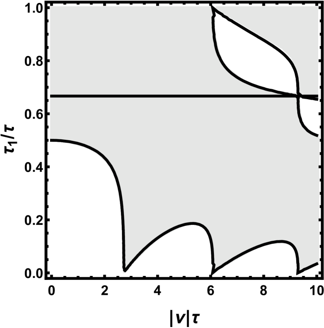
Figure 5: For a given value of the Raman detuning $\nu$, the duration of the first and third rectangular pulses should be in the gray area. The straight line corresponds to pulses of equal duration, $\tau_{1}=\tau_{2}=\tau_{3}=\dfrac{2}{3}\tau,$ when the solution of the Eq. (102) exists for any $\nu$.

The solution of the Eq. (102) is given by

$$\tau_{b} = \dfrac{1}{2}\tau^{\left(3_{\pm}\right)}\left(j,\nu\right),$$ (103a)

$$\tau^{\left(3_{\pm}\right)}\left(j,\nu\right) = \dfrac{2}{\nu}\left[\pm\arccos\dfrac{\left|s_{a2}\right|\left(\left|s_{a1}\right|^{2}-\left|s_{d1}\right|^{2}\right)}{2\left|s_{a1}s_{d1}s_{d2}\right|}-\arctan\dfrac{\mathop{\mathrm{I}m}\left(s_{d1}s_{d2}\right)}{\mathop{\mathrm{R}e}\left(s_{d1}s_{d2}\right)}+2j\pi\right],$$ (103b)

where for each value of $$\nu j \tau_{b}>0$$ the integer can take only those values for which . Hence, the wave function of the atom in the ground state, after the action of the NCP acquires the phase factor

$$s_{gg} = \exp\left[i\eta_{0}^{\left(3_{\pm}\right)}+i\eta_{0}^{\left(3_{\pm}\right)}\left(\nu\right)\right],$$ (104a)

$$\eta_{0}^{\left(3_{\pm}\right)} = \pi,$$ (104b)

$$\eta_{0}^{\left(3_{\pm}\right)}\left(\nu\right) = -\arctan\left(\dfrac{2\tau\nu}{\sqrt{\pi^{2}+4\nu^{2}\tau^{2}}}\tan\dfrac{\tau_{1}}{4\tau}\sqrt{\pi^{2}+4\nu^{2}\tau^{2}}\right)\pm\arccos\dfrac{1}{2}\left|\dfrac{s_{a2}}{s_{a1}s_{d1}}\right|.$$ (104c)

To calculate linear in $$\nu^{\left(1\right)}$$ corrections, one can use the equality (92), in which one should make the substitution

$$\tau^{\left(2\right)}\left(j,\nu\right)\rightarrow\dfrac{1}{2}\tau^{\left(3_{\pm}\right)}\left(j,\nu\right).$$ (105)

From Eqs. (104a, 100) follows, respectively, that

$$\dfrac{d}{d\nu}\left.s_{gg}\right|_{\tau_{b}=0.5\tau^{\left(3_{\pm}\right)}\left(j,\nu\right)} = i\dfrac{d\eta_{0}^{\left(3_{\pm}\right)}\left(\nu\right)}{d\nu}\left.s_{gg}\right|_{\tau_{b}=0.5\tau^{\left(3_{\pm}\right)}\left(j,\nu\right)},$$ (106a)

$$\left.\dfrac{\partial s_{gg}}{\partial\tau_{b}}\right|_{\tau_{b}=0.5\tau^{\left(3_{\pm}\right)}\left(j,\nu\right)} = i\nu\left(\left|s_{a1}\right|^{2}-\left|s_{d1}\right|^{2}\right)\left.s_{gg}\right|_{\tau_{b}=0.5\tau^{\left(3_{\pm}\right)}\left(j,\nu\right)}.$$ (106b)

These expressions allow one to extract $$s_{gg}^{\prime} \delta s_{gg} s_{eg},$$ from Eq. (92) [taking into account the replacement (105)] and get . Computing the off-diagonal element in a similar way, one arrives at the following result

$$\underline{s}=$$

$$\left(\begin{array}[]{cc}\exp\left[-i\eta_{0}^{\left(3_{\pm}\right)}-i\eta_{0}^{\left(3_{\pm}\right)}\left(\nu\right)-i\eta_{1}^{\left(3_{\pm}\right)}\left(\nu\right)\nu_{1}\right]&\mp i\exp\left(i\arg\Omega\right)\dfrac{d\tau^{\left(3_{\pm}\right)}}{d\nu}\sqrt{4\left|s_{a1}\right|^{2}\left|s_{d1}\right|^{2}-\left|s_{a2}\right|^{2}}\nu^{\left(0\right)}\nu^{\left(1\right)}\\ \mp i\exp\left(-i\arg\Omega\right)\dfrac{d\tau^{\left(3_{\pm}\right)}}{d\nu}\sqrt{4\left|s_{a1}\right|^{2}\left|s_{d1}\right|^{2}-\left|s_{a2}\right|^{2}}\nu^{\left(0\right)}\nu^{\left(1\right)}&\exp\left[i\eta_{0}^{\left(3_{\pm}\right)}+i\eta_{0}^{\left(3_{\pm}\right)}\left(\nu\right)+i\eta_{1}^{\left(3_{\pm}\right)}\left(\nu\right)\nu_{1}\right]\end{array}\right),$$ (107c)

$$\eta_{1}^{\left(3_{\pm}\right)}\left(\nu\right)=\dfrac{d\eta_{0}^{\left(3_{\pm}\right)}\left(\nu\right)}{d\nu}-\dfrac{\nu}{2}\left(\left|s_{a1}\right|^{2}-\left|s_{d1}\right|^{2}\right)\dfrac{d\tau^{\left(3_{\pm}\right)}\left(j,\nu\right)}{d\nu}.$$ (107d)

From Eqs. (58, 73) the total NCP duration is given by

$$\tau\left(\nu,\zeta,\beta,1\right) = \pi\dfrac{\sqrt{4j_{\zeta,\beta,1}^{2}-1}}{\left|\nu\right|}$$ (108a)

$$\tau\left(\nu,\zeta,\beta,2\right) = 2\tau+\tau^{\left(2\right)}\left(j_{\zeta,\beta,2},\nu\right),$$ (108b)

$$\tau\left(\nu,\zeta,\beta,3_{\pm}\right) = 2\tau+\tau^{\left(3_{\pm}\right)}\left(j_{\zeta,\beta,3_{\pm}},\nu\right),$$ (108c)

where $$\tau^{\left(2\right)}\left(j,\nu\right) \tau^{\left(3_{\pm}\right)}\left(j,\nu\right)$$ and are given in Eqs. (90, 103b) respectively.

III The phase

Consider the interaction of an atomic cloud with a sequence of three main resonant Raman pulses $\pi/2-\pi-\pi/2$, acting at the moments $\left\{T_{1,0},T_{2,0},T_{3,0}\right\}$, having duration $\tau-2\tau-\tau$ and effective wave vector $\mathbf{k}$. Suppose that the atom was launched at $t=0$ in the ground state, i.e. at $t<T_{1,0}$

$$c\left(e,\mathbf{p},t\right) = 0,$$ (109a)

$$c\left(g,\mathbf{p},t\right) = \sqrt{f_{g}\left(\mathbf{p}\right)},$$ (109b)

where $$f_{g}\left(\mathbf{p}\right) \sqrt{f_{g}\left(\mathbf{p}\right)} \pi- 2n \left\{\zeta,\beta\right\} 1\leq\zeta\leq 3 \left\{\zeta,0\right\} \zeta=1 1\leq\beta\leq 2n \pi/2- \zeta=2 -2n\leq\beta\leq-1 1\leq\beta\leq 2n \pi- \zeta=3 -2n\leq\beta\leq-1 \pi/2- 1\leq\ell_{\zeta,\beta}\leq 3$$ is the momentum distribution function in the atomic cloud. Below, up to Eq. (138), to simplify the calculation, we omit the factor . Regarding the auxiliary Raman pulses, we will assume that there are an even number of them, , in each of the four sets. All pulses, main and auxiliary, are numbered with integers , where . The numbers of the main pulses are , and for the auxiliary NCPs at the values correspond to the set following the first main pulse, at the values and correspond to the pulses that preceded or followed after the second main pulse, with the values correspond to the set preceding the third main pulse. Each of the pulses is NCP, consisting of rectangular pulses. The effective wave vector and momentum chirp rate are

$$\mathbf{k}_{\zeta,\beta} = \left(-1\right)^{\beta}\mathbf{k},$$ (110a)

$$\alpha_{\zeta,\beta} = \left(-1\right)^{\beta}\alpha$$ (110b)

and its total duration $$\tau\left(\nu,\zeta,\beta,\ell_{\zeta,\beta}\right)$$ for auxiliary NCPs is given in Eqs. (108), and for the main ones there are

$$\tau\left(0,1,0,1\right)=\tau\left(0,2,0,1\right)/2=\tau\left(0,3,0,1\right)=\tau,$$ (111)

here one takes into account that the main pulses are resonant for the blue and red branches of the recoil diagram, i.e. for them $\nu^{\left(0\right)}=0$. In our calculations, we take into account the finite durations of the Raman pulses. For their timing, following Ref. i29 , we introduce a delay time between pulses

$$d_{\zeta,m}\equiv\left\{\begin{array}[]{c}T_{\zeta,m}-T_{\zeta,m-1}-\tau\left(\nu,\zeta,m-1,\ell_{\zeta,m-1}\right),\text{ for }-2n<m\leq 2n\\ T\equiv T_{\zeta,-2n}-T_{\zeta-1,2n}-\tau\left(\nu,\zeta-1,2n,\ell_{\zeta-1,2n}\right),\text{ for }m=-2n,\zeta>1\end{array}\right.,$$ (112)

i.e., we define the interrogation time $T$ as the time between the end of the last auxiliary NCP $\left\{1,2n\right\}$ and the beginning of the first auxiliary NCP $\left\{2,-2n\right\}$, which coincides with the time between the end of the last auxiliary NCP $\left\{2,2n\right\}$ and the beginning of the first auxiliary NCP $\left\{3,-2n\right\}$. From the given $T_{1,0}$, delays between NCPs (112) and their durations (108, 111) one can make up the full timing , the moments of action of each of the pulses $T_{\zeta,\beta}$. One can represent them as

$$T_{\zeta,\beta}=T_{\zeta,\beta}^{\left(0\right)}+\Upsilon_{\zeta,\beta},$$ (113)

where $T_{\zeta,\beta}^{\left(0\right)}$ is $T_{1,0}$ plus the sum of all preceding delays, while $\Upsilon_{\zeta,\beta}$ is the sum of the durations of all preceding pulses.

In this article, we neglect the deviations of pulses from the ideal shape and duration calculated below. Therefore, the gray lines on the recoil diagram associated with these deviations do not appear. We also assume negligible diagonal elements in $s-$matrices (77, 85, 96) and off-diagonal elements in $s-$matrices (76c, 94c, 107c). So the gray lines associated with the finite duration of the Raman pulses do not appear either. As a result, only two branches, blue and red, remain on the recoil diagram. In this case, the wave function of an atom is a column,

$$\underline{\chi}=\left(\begin{array}[]{c}\chi_{b}\\ \chi_{r}\end{array}\right).$$ (114)

After the action of $\pi/2-$pulse $\left\{1,0\right\}$ from Eqs. (61, 109) one will find that this column is

$$\left(\begin{array}[]{c}c\left(e,\mathbf{p}_{+}^{\left(1,0\right)}+\hbar\mathbf{k},T_{1,0}+\tau\right)\\ c\left(g,\mathbf{p}_{+}^{\left(1,0\right)},T_{1,0}+\tau\right)\end{array}\right)=\left(\begin{array}[]{c}S_{eg}^{\left(1,0\right)}\left(\mathbf{p}_{+,T_{1,0}+\tau}^{\left(1,0\right)}+\hbar\mathbf{k}/2\right)\\ S_{gg}^{\left(1,0\right)}\left(\mathbf{p}_{+,T_{1,0}+\tau}^{\left(1,0\right)}+\hbar\mathbf{k}/2\right)\end{array}\right),$$ (115)

where the matrix $S\left(\mathbf{P}\right)$ is given in Eq. (62c). At resonance, when

$$\nu_{r}^{\left(0\right)}=\delta_{1,0}^{\left(0\right)}\left(\mathbf{p}_{+,T_{1,0}+\tau}^{\left(1,0\right)}+\hbar\mathbf{k}/2\right)=\delta_{1,0}-\dfrac{\mathbf{k}}{M}\mathbf{\cdot p}_{+,T_{1,0}+\tau}^{\left(1,0\right)}-\omega_{k}\approx 0$$ (116)

and $\left|\Omega_{1,0}\right|$ given in Eq. (78), from Eqs. (56d, 46a, 46d, 75a) it follows, respectively, that

$$\underline{s} = \dfrac{1}{\sqrt{2}}\left(\begin{array}[]{cc}1&-i\exp\left(i\arg\Omega_{1,0}\right)\\ -i\exp\left(i\arg\Omega_{1,0}\right)&1\end{array}\right),$$ (117c)

$$\nu_{r}^{\left(0\right)} = \delta_{1,0}-\dfrac{\mathbf{k}}{M}\cdot\mathbf{p}_{+,T_{1,0}+\tau}^{\left(1,0\right)}-\omega_{k}$$ (117d)

$$\nu_{r} = -\left(\mathbf{k\cdot g}-\alpha\right)T_{1,0},$$ (117e)

$$\phi_{1,0}\left(\mathbf{p}_{+,T_{1,0}+\tau}^{\left(1,0\right)}+\hbar\mathbf{k}/2\right) = \phi_{1,0}+\left(\delta_{1,0}-\dfrac{\mathbf{k}}{M}\mathbf{\cdot p}_{+,T_{1,0}+\tau}^{\left(1,0\right)}-\omega_{k}\right)T_{1,0}-\dfrac{1}{2}\left(\mathbf{k\cdot g}-\alpha\right)T_{1,0}^{2},$$ (117f)

$$s_{d}^{\prime} = \dfrac{i\sqrt{2}}{\pi},$$ (117g)

Despite the resonance, we retained the Ramsey term i28 [the second term in the expression for the phase (117f)]. For resonance it is enough that

$$\left|\nu_{r}^{\left(0\right)}\right|\ll\tau^{-1}.$$ (118)

If

$$T_{1,0}\sim T\gg\tau,$$ (119)

then, despite the resonance condition, one can observe Ramsey fringes at

$$T^{-1}\lesssim\left|\nu_{r}^{\left(0\right)}\right|\ll\tau^{-1}.$$ (120)

From Eqs.. (115, 62, 117) one gets

$$\left(\begin{array}[]{c}c\left(e,\mathbf{p}_{+}^{\left(1,0\right)}+\hbar\mathbf{k},T_{1,0}+\tau\right)\\ c\left(g,\mathbf{p}_{+}^{\left(1,0\right)},T_{1,0}+\tau\right)\end{array}\right)=\dfrac{1}{\sqrt{2}}\left(\begin{array}[]{c}\exp\left(i\psi_{1,0}^{\left(b\right)}\right)\\ \exp\left(i\psi_{1,0}^{\left(r\right)}\right)\end{array}\right),$$ (121e)

$$\psi_{1,0}^{\left(b\right)}=-\dfrac{\pi}{2}-\phi_{1,0}+\arg\Omega_{1,0}-\left(\delta_{1,0}-\dfrac{\mathbf{k}}{M}\cdot\mathbf{p}_{+,T_{1,0}+\tau}^{\left(1,0\right)}-\omega_{k}\right)T_{1,0}+\dfrac{1}{2}\left(\mathbf{k\cdot g}-\alpha\right)T_{1,0}^{2}+\dfrac{1}{2}\left(\mathbf{k\cdot g}-\alpha\right)T_{1,0}\tau,$$ (121f)

$$\psi_{1,0}^{\left(r\right)}=\left(\dfrac{2}{\pi}-\dfrac{1}{2}\right)\left(\mathbf{k\cdot g}-\alpha\right)T_{1,0}\tau.$$ (121g)

meaning 4 With the exception of the last beam splitter $$\left\{3,0\right\} \pi- \pi-$$, all subsequent beam splitters are pulses. An ideal pulse does not change the magnitude of states, only the phases of these states change. These changes, phase augmentations, in sum determine the phase of the interferometer.meaning 4

Let us now consider the action of an odd NCP $\left\{1,2m-1\right\}$, for which $\mathbf{k}_{1,2m-1}=-\mathbf{k}.$ Before interaction

$$\underline{\chi}=\left(\begin{array}[]{c}c\left(e,\mathbf{\pi}_{-},T_{1,2m-1}\right)\\ c\left(g,\mathbf{p}_{-}^{\left(1,2m-1\right)},T_{1,2m-1}\right)\end{array}\right)=\dfrac{1}{\sqrt{2}}\left(\begin{array}[]{c}\exp\left(i\psi_{1,2m-2}^{\left(b\right)}\right)\\ \exp\left(i\psi_{1,2m-2}^{\left(r\right)}\right)\end{array}\right).$$ (122)

From the recoil diagrams in Figs. 2, 3, one can conclude that on the resonant branch, for arbitrary $m$, the preceding Raman pulses transferred to the atom an odd number of momenta $\hbar\mathbf{k}$, i.e.

$$\mathbf{\pi}_{-}=\mathbf{p}_{-}^{\left(1,2m-1\right)}+\left(2m-1\right)\hbar\mathbf{k}$$ (123)

Then, along the blue resonance branch after the NCP, from Eqs. (64b, 110a) for $\mathfrak{N}=2m$ the state of the atom changes as

$$c\left(g,\mathbf{\pi}_{+},T_{1,2m-1}+\tau_{p}\right) = S_{ge}^{\left(1,2m-1\right)}\left(\mathbf{\pi}_{s}\right)c\left(e,\mathbf{\pi}_{-},T_{1,2m-1}\right)$$ (124a)

$$\mathbf{\pi}_{+} = \mathbf{p}_{+}^{\left(1,2m-1\right)}+2m\hbar\mathbf{k},$$ (124b)

$$\tau_{p} = \tau\left(\nu,1,2m-1,\ell_{1,2m-1}\right)$$ (124c)

$$\mathbf{\pi}_{s} = \mathbf{\pi+}\left(4m-1\right)\hbar\mathbf{k}/2,$$ (124d)

$$\mathbf{\pi} = \mathbf{p}_{+,T_{1,2m-1}+\tau_{p}}^{\left(1,2m-1\right)}$$ (124e)

In this case, under the condition of resonance

$$\nu_{r}^{\left(0\right)}=\delta_{1,2m-1}^{\left(0\right)}\left(\mathbf{\pi}_{s}\right)=\left\{\delta_{1,2m-1}+\dfrac{\mathbf{k}}{M}\mathbf{\cdot\pi}\right\}+\left(4m-1\right)\omega_{k}\approx 0,$$ (125a)

$$\nu_{r}=\left(\mathbf{k\cdot g}-\alpha\right)T_{1,2m-1},$$ (125b)

$$\phi_{1,2m-1}\left(\mathbf{\pi}_{s}\right)=\phi_{1,2m-1}+\left[\delta_{1,2m-1}+\dfrac{\mathbf{k}}{M}\mathbf{\cdot\pi}+\left(4m-1\right)\omega_{k}\right]T_{1,2m-1}+\dfrac{1}{2}\left(\mathbf{k\cdot g}-\alpha\right)T_{1,2m-1}^{2},$$ (125c)

and then, using the off-diagonal matrix element in the $$s-$$matrices (77, 83, 96), from Eqs.. (124, 62, 125) one receives

$$c\left(g,\mathbf{\pi}_{+},T_{1,2m-1}+\tau_{p}\right)=\dfrac{1}{\sqrt{2}}\exp\left(i\psi_{1,2m-1}^{\left(b\right)}\right),$$ (126a)

$$\psi_{1,2m-1}^{\left(b\right)}=\psi_{1,2m-2}^{\left(b\right)}+A_{1,2m-1}^{\left(b\right)},$$ (126b)

$$A_{1,2m-1}^{\left(b\right)}=-\dfrac{\pi}{2}+\phi_{1,2m-1}-\arg\Omega_{1,2m-1}+\left[\delta_{1,2m-1}+\dfrac{\mathbf{k}}{M}\mathbf{\cdot\pi}+\left(4m-1\right)\omega_{k}\right]T_{1,2m-1}^{\left(0\right)}$$

$$+\dfrac{1}{2}\left(\mathbf{k\cdot g}-\alpha\right)T_{1,2m-1}^{2}+\dfrac{1}{2}\left(\mathbf{k\cdot g}-\alpha\right)T_{1,2m-1}^{\left(0\right)}\tau_{p},$$ (126c)

where $$A_{1,2m-1}^{\left(b\right)} \left\{1,2m-1\right\}$$ is the phase augmentation of the atomic amplitude on the blue branch during interaction with the NCP . In the expression (126c) we have replaced

$$T_{\zeta,\beta}\rightarrow T_{\zeta,\beta}^{\left(0\right)}$$ (127)

in the 4th and last term. This is because in the resonance condition (118)

$$\left|\nu_{r}\right|\Upsilon_{\zeta,\beta}\ll 1.$$ (128)

We also took into account that one can neglect the term $\Upsilon_{\zeta,\beta}\tau$ since it is bilinear in pulse durations.

Consider now the nonresonant red branch, where

$$c\left(g,\mathbf{p}_{+}^{\left(1,2m-1\right)},T_{1,2m-1}+\tau_{p}\right)=S_{gg}^{\left(1,2m-1\right)}\left(\mathbf{\pi}-\hbar\mathbf{k}/2\right)c\left(g,\mathbf{p}_{-}^{\left(1,2m-1\right)},T_{1,2m-1}\right).$$ (129)

From Eqs. (46, 125a) one finds

$$\nu=\delta_{1,2m-1}\left(\mathbf{\pi}-\hbar\mathbf{k}/2\right)=\left\{\delta_{1,2m-1}+\dfrac{\mathbf{k}}{M}\mathbf{\cdot\pi}\right\}-\omega_{k}+\left(\mathbf{k\cdot g}-\alpha\right)T_{1,2m-1}.$$ (130)

Since terms in curly brackets in Eqs. (125a, 130) coincide, then

$$\nu=-4m\omega_{k}+\left(\mathbf{k\cdot g}-\alpha\right)T_{1,2m-1}.$$ (131)

meaning 4 Thus, knowing that there is no frequency detuning on the resonant branch of the recoil diagram, one is able to determine the detuning $\nu$ on the nonresonant branch. Since at a negligibly small recoil frequency there is no detuning on both branches, then at $\omega_{k}\neq 0$ the detuning $\nu$ is determined only by the recoil frequency and the Doppler frequency shift does not contribute to it.meaning 4

The second term in Eq.(131) is a small correction associated with the finite duration of the NCP. One sees that in order to fulfill the requirement 2, the total duration of the NCP must be equal to

$$\tau_{p}=\tau\left(-4m\omega_{k},1,2m-1,\ell_{1,2m-1}\right)$$ (132)

given by Eqs. (108). Then using the matrix element $s_{gg}$ $s-$matrices (76c, 94c, 107c), from Eqs. (129, 62, 131) one finds that

$$c\left(g,\mathbf{p}_{+}^{\left(1,2m-1\right)},T_{1,2m-1}+\tau_{p}\right)=\dfrac{1}{\sqrt{2}}\exp\left(i\psi_{1,2m-1}^{\left(r\right)}\right),$$ (133a)

$$\psi_{1,2m-1}^{\left(r\right)}=\psi_{1,2m-2}^{\left(r\right)}+A_{1,2m-1}^{\left(r\right)},$$ (133b)

$$A_{1,2m-1}^{\left(r\right)}=-2m\omega_{k}\tau_{p}+\eta_{0}^{\left(\ell_{1,2m-1}\right)}+\eta_{0}^{\left(\ell_{1,2m-1}\right)}\left(-4m\omega_{k}\right)+\left[\dfrac{1}{2}\tau_{p}+\eta_{1}^{\left(\ell_{1,2m-1}\right)}\left(-4m\omega_{k}\right)\right]\left(\mathbf{k\cdot g}-\alpha\right)T_{1,2m-1}^{\left(0\right)},$$ (133c)

where $$\eta_{0}^{\left(\ell_{1,2m-1}\right)}$$ is given by Eqs. (76d, 91b, 104b),

$$\eta_{0}^{\left(1\right)}\left(\nu\right)=0,$$ (134)

$\eta_{0}^{\left(2\right)}\left(\nu\right)$ and $\eta_{0}^{\left(3_{\pm}\right)}\left(\nu\right)$ are respectively given by Eqs. (91c, 104c$>$), $\eta_{1}^{\left(\ell\right)}\left(\nu\right)$ are given by Eqs. (76e, 94d, 107d). In the last term, we also made a replacement (127).

The action of the remaining $\pi-$pulses can be calculated in a similar way. One can verify that the ideal $\pi-$pulse $\left\{\zeta,\beta\right\}$, for which one assigns the duration exactly according to the expressions (108), and which is in resonance with atomic transitions with an accuracy much less than the inverse pulse duration, leads only to phase augmentation of the atomic states amplitudes, $A_{\zeta,\beta}^{\left(b,r\right)}$. One arrives at the following expressions for these augmentations

$$A_{1,m}^{\left(b\right)}=-\dfrac{\pi}{2}-\left(-1\right)^{m}\left(\phi_{1,m}-\arg\Omega_{1,m}\right)-\left[\left(-1\right)^{m}\delta_{1,m}-\dfrac{\mathbf{k}}{M}\mathbf{\cdot\pi}-\left(2m+1\right)\omega_{k}\right]T_{1,m}^{\left(0\right)}$$

$$+\dfrac{1}{2}\left(\mathbf{k\cdot g}-\alpha\right)T_{1,m}^{2}+\dfrac{1}{2}\left(\mathbf{k\cdot g}-\alpha\right)T_{1,m}^{\left(0\right)}\tau_{p},$$ (135a)

$$A_{1,m}^{\left(r\right)}=\left(-1\right)^{m}\xi_{m}\omega_{k}\tau_{p}+\eta_{0}^{\left(\ell_{1,m}\right)}+\eta_{0}^{\left(\ell_{1,m}\right)}\left[\left(-1\right)^{m}2\xi_{m}\omega_{k}\right]-\left(-1\right)^{m}\left\{\dfrac{1}{2}\tau_{p}+\eta_{1}^{\left(\ell_{1,m}\right)}\left[\left(-1\right)^{m}2\xi_{m}\omega_{k}\right]\right\}\left(\mathbf{k\cdot g}-\alpha\right)T_{1,m}^{\left(0\right)},$$ (135b)

$$A_{2,-m}^{\left(b\right)}=-\dfrac{\pi}{2}+\left(-1\right)^{m}\left(\phi_{2,-m}-\arg\Omega_{2,-m}\right)+\left[\left(-1\right)^{m}\delta_{2,-m}-\dfrac{\mathbf{k}}{M}\mathbf{\cdot\pi}-\left(2m+1\right)\omega_{k}\right]T_{2,-m}^{\left(0\right)}$$

$$-\dfrac{1}{2}\left(\mathbf{k\cdot g}-\alpha\right)T_{2,-m}^{2}-\dfrac{1}{2}\left(\mathbf{k\cdot g}-\alpha\right)T_{2,-m}^{\left(0\right)}\tau_{p},$$ (135c)

$$A_{2,-m}^{\left(r\right)}=\left(-1\right)^{m}\xi_{m}\omega_{k}\tau_{p}+\eta_{0}^{\left(\ell_{2,-m}\right)}+\eta_{0}^{\left(\ell_{2,-m}\right)}\left(\left(-1\right)^{m}2\xi_{m}\omega_{k}\right)-\left(-1\right)^{m}\left[\dfrac{1}{2}\tau_{p}+\eta_{1}^{\left(\ell_{2,-m}\right)}\left(\left(-1\right)^{m}2\xi_{m}\omega_{k}\right)\right]\left(\mathbf{k\cdot g}-\alpha\right)T_{2,-m}^{\left(0\right)},$$ (135d)

$$A_{2,0}^{\left(b\right)}=-\dfrac{\pi}{2}+\phi_{2,0}-\arg\Omega_{2,0}+\left[\delta_{2,0}-\dfrac{\mathbf{k}}{M}\mathbf{\cdot p}_{+,T_{2,0}+2\tau}^{\left(2,0\right)}-\omega_{k}\right]T_{2,0}^{\left(0\right)}-\dfrac{1}{2}\left(\mathbf{k\cdot g}-\alpha\right)T_{2,0}^{2}-\left(\mathbf{k\cdot g}-\alpha\right)T_{2,0}^{\left(0\right)}\tau,$$ (135e)

$$A_{2,0}^{\left(r\right)}=-\pi-A_{2,0}^{\left(b\right)},$$ (135f)

$$A_{2,m}^{\left(b\right)}=\left(-1\right)^{m}\xi_{m}\omega_{k}\tau_{p}+\eta_{0}^{\left(\ell_{2,m}\right)}+\eta_{0}^{\left(\ell_{2,m}\right)}\left(\left(-1\right)^{m}2\xi_{m}\omega_{k}\right)-\left(-1\right)^{m}\left[\dfrac{1}{2}\tau_{p}+\eta_{1}^{\left(\ell_{2,m}\right)}\left(\left(-1\right)^{m}2\xi_{m}\omega_{k}\right)\right]\left(\mathbf{k\cdot g}-\alpha\right)T_{2,m}^{\left(0\right)},$$ (135g)

$$A_{2,m}^{\left(r\right)}=-\dfrac{\pi}{2}-\left(-1\right)^{m}\left(\phi_{2,m}-\arg\Omega_{2,m}\right)-\left[\left(-1\right)^{m}\delta_{2,m}-\dfrac{\mathbf{k}}{M}\mathbf{\cdot\pi}-\left(2m+1\right)\omega_{k}\right]T_{2,m}^{\left(0\right)}$$

$$+\dfrac{1}{2}\left(\mathbf{k\cdot g}-\alpha\right)T_{2,m}^{2}+\dfrac{1}{2}\left(\mathbf{k\cdot g}-\alpha\right)T_{2,m}^{\left(0\right)}\tau_{p},$$ (135h)

$$A_{3,-m}^{\left(b\right)}=\left(-1\right)^{m}\xi_{m}\omega_{k}\tau_{p}+\eta_{0}^{\left(\ell_{3,-m}\right)}+\eta_{0}^{\left(\ell_{3,-m}\right)}\left(\left(-1\right)^{m}2\xi_{m}\omega_{k}\right)-\left(-1\right)^{m}\left[\dfrac{1}{2}\tau_{p}+\eta_{1}^{\left(\ell_{3,-m}\right)}\left(\left(-1\right)^{m}2\xi_{m}\omega_{k}\right)\right]\left(\mathbf{k\cdot g}-\alpha\right)T_{3,-m}^{\left(0\right)},$$ (135i)

$$A_{3,-m}^{\left(r\right)}=-\dfrac{\pi}{2}+\left(-1\right)^{m}\left(\phi_{3,-m}-\arg\Omega_{3,-m}\right)+\left[\left(-1\right)^{m}\delta_{3,-m}-\dfrac{\mathbf{k}}{M}\mathbf{\cdot\pi}-\left(2m+1\right)\omega_{k}\right]T_{3,-m}^{\left(0\right)}$$

$$-\dfrac{1}{2}\left(\mathbf{k\cdot g}-\alpha\right)T_{3,-m}^{2}-\dfrac{1}{2}\left(\mathbf{k\cdot g}-\alpha\right)T_{3,-m}^{\left(0\right)}\tau_{p},$$ (135j)

where

$$\xi_{m}=m+\dfrac{1}{2}\left(1-\left(-1\right)^{m}\right).$$ (136)

In the expressions for augmentations $A_{\zeta,\beta}^{\left(b,r\right)}$ the duration of the pulse $\left\{\zeta,\beta\right\}$ $\tau_{p}$ and momentum $\mathbf{\pi}$ are given by

$$\tau_{p} = \tau\left[\left(-1\right)^{\beta}2\xi_{\beta}\omega_{k},\zeta,\beta,\ell_{\zeta,\beta}\right],$$ (137a)

$$\mathbf{\pi} \mathbf{=} \mathbf{p}_{+,T_{\zeta,\beta}+\tau_{p}}^{\left(\zeta,\beta\right)}$$ (137b)

meaning4.5Augmentations (135a, 135c, 135e, 135f, 135h, 135j) refer to the resonant branch of the recoil diagram, while augmentations (135b, 135d, 135g, 135i) refer to the nonresonant branch.meaning4.5The factor $$(-1)^{m} g\rightarrow e e\rightarrow g S \delta g\rightarrow e e\rightarrow g \pm\mathbf{k.}$$ reflects the fact that at the transitions and one uses different offdiagonal elements of the matrix in Eq. (62), and for them the signs of the phase factors are opposite. As a result, the terms associated with the detuning change sign. But at the same time, the terms associated with the Doppler shift and the gravitational field remain unchanged, because for transitions and one uses opposite effective wave vectors

Using augmentations (135), one calculates the phases of the atomic states amplitudes before the action of the third main $\pi/2-$pulse, $\left\{\psi_{3,-1}^{\left(b\right)},\psi_{3,-1}^{\left(r\right)}\right\}$. We are interested in the total probability of excitation of atoms in the cloud

$$w=\int d\mathbf{p}_{+}^{\left(3,0\right)}f_{g}\left[\mathbf{p}_{+}^{\left(3,0\right)}\right]\left|c\left(e,\mathbf{p}_{+}^{\left(3,0\right)}+\hbar\mathbf{k},T_{3,0}+\tau\right)\right|^{2},$$ (138)

where we have restored the factor $\sqrt{f_{g}\left(\mathbf{p}\right)}$ from Eq. (109b). At $t=T_{3,0}+\tau$ the amplitude of an atom in an excited state consists of blue and red components,

$$c\left(e,\mathbf{p}_{+}^{\left(3,0\right)}+\hbar\mathbf{k},T_{3,0}+\tau\right)=c^{\left(b\right)}\left(e,\mathbf{p}_{+}^{\left(3,0\right)}+\hbar\mathbf{k},T_{3,0}+\tau\right)+c^{\left(r\right)}\left(e,\mathbf{p}_{+}^{\left(3,0\right)}+\hbar\mathbf{k},T_{3,0}+\tau\right),$$ (139)

for which one has

$$c^{\left(b\right)}\left(e,\mathbf{p}_{+}^{\left(3,0\right)}+\hbar\mathbf{k},T_{3,0}+\tau\right) = S_{eg}^{\left(3,0\right)}\left(\mathbf{p}_{+,T_{3,0}+\tau}^{\left(3,0\right)}+\hbar\mathbf{k}/2\right)c\left(g,\mathbf{p}_{-}^{\left(3,0\right)},T_{3,0}\right),$$ (140a)

$$c^{\left(r\right)}\left(e,\mathbf{p}_{+}^{\left(3,0\right)}+\hbar\mathbf{k},T_{3,0}+\tau\right) = S_{ee}^{\left(3,0\right)}\left(\mathbf{p}_{+,T_{3,0}+\tau}^{\left(3,0\right)}+\hbar\mathbf{k}/2\right)c\left(e,\mathbf{p}_{-}^{\left(3,0\right)}+\hbar\mathbf{k},T_{3,0}\right).$$ (140b)

After calculations similar to those used in the derivation of Eqs. (121), one obtains

$$\left(\begin{array}[]{c}c^{\left(b\right)}\left(e,\mathbf{p}_{+}^{\left(3,0\right)}+\hbar\mathbf{k},T_{3,0}+\tau\right)\\ c^{\left(r\right)}\left(e,\mathbf{p}_{+}^{\left(3,0\right)}+\hbar\mathbf{k},T_{3,0}+\tau\right)\end{array}\right)=\dfrac{1}{2}\left(\begin{array}[]{c}\exp\left(i\psi_{3,0}^{\left(b\right)}\right)\\ \exp\left(i\psi_{3,0}^{\left(r\right)}\right)\end{array}\right);$$ (141e)

$$\psi_{3,0}^{\left(b,r\right)}=\psi_{3,-1}^{\left(b,r\right)}+A_{3,0}^{\left(b,r\right)},$$ (141f)

$$A_{3,0}^{\left(b\right)}=-\dfrac{\pi}{2}-\phi_{3,0}+\arg\Omega_{3,0}-\left[\delta_{3,0}-\dfrac{\mathbf{k}}{M}\mathbf{\cdot p}_{+,T_{3,0}+\tau}^{\left(3,0\right)}-\omega_{k}\right]T_{3,0}^{\left(0\right)}+\dfrac{1}{2}\left(\mathbf{k\cdot g}-\alpha\right)T_{3,0}^{2}+\dfrac{1}{2}\left(\mathbf{k\cdot g}-\alpha\right)T_{3,0}\tau,$$ (141g)

$$A_{3,0}^{\left(r\right)}=\left(\dfrac{1}{2}-\dfrac{2}{\pi}\right)\left(\mathbf{k\cdot g}-\alpha\right)T_{3,0}^{\left(0\right)}\tau.$$ (141h)

In Eqs. (139) the independent variable is the momentum of the atom after the action of the pulse $\left\{3,0\right\}$, $\mathbf{p}_{+}^{\left(3,0\right)}$. Using Eqs. (65, 66b) one can calculate the values of all other momenta in Eqs. (135). Such calculations would be necessary if we were only interested in one of the ports on Figs. 1-3. The total excitation probability (138) is the sum of the probabilities over all possible ports. And for this response, in Eq. (138), one introduces a new integration variable

$$\mathbf{p}_{i}=\mathbf{p}_{+,T_{3,0}+\tau}^{\left(3,0\right)}.$$ (142)

From Eq. (60b) it follows that all pulses in Eqs. (135) coincide with $\mathbf{p}_{i}$.meaning 5 This coincidence is a consequence of the fact that in Eq. (63) one selected in the momentum the parts associated with the transfer of photon momenta $\mathfrak{N\hbar}\mathbf{k}$, and the momentum that changes only under the action of the gravitational field.meaning 5

Integrand in Eq. (138) is a rapidly oscillating function momentum $\mathbf{p}_{i}$ with a period of the order of $M/kT$. One chooses the timing of the pulses in the AI such that these oscillations disappear. If, in addition, the atomic cloud is cooled to such a temperature that the momentum in the functions of the parameters $s_{d}$ and $s_{a}$ from Eqs. (56) can be considered to be the same as the average momentum in the cloud, then one will receive

$$w=\dfrac{1}{2}\left(1-\cos\phi\right),$$ (143)

where the phase of the atomic interferometer is

$$\phi = \pi+\psi_{3,0}^{\left(b\right)}-\psi_{3,0}^{\left(r\right)}=\pi+\mathop{\displaystyle\sum}_{j=1}^{3}A_{j,0}+\mathop{\displaystyle\sum}_{m=1}^{2n}\left(A_{1,m}+A_{2,-m}+A_{2,m}+A_{3,-m}\right),$$ (144a)

$$A_{\zeta,\beta} \equiv \left\{\begin{array}[]{c}\psi_{1,0}^{\left(b\right)}-\psi_{1,0}^{\left(r\right)},\text{ for }\left\{\zeta,\beta\right\}=\left\{1,0\right\}\\ A_{\zeta,\beta}^{\left(b\right)}-A_{\zeta,\beta}^{\left(r\right)},\text{ for }\left\{\zeta,\beta\right\}\not=\left\{1,0\right\}\end{array}\right..$$ (144d)

Then from Eqs. (121f, 121g, 135, 141g, 141h) one arrives at the next result

$$\phi=\bar{\phi}+\phi_{R}+\phi_{D}+\phi_{q}+\bar{\phi}_{q}+\phi_{g}^{\left(0\right)}+\phi_{g}^{\left(1\right)},$$ (145)

where

$$\bar{\phi}=-\phi_{1,0}+2\phi_{2,0}-\phi_{3,0}-\mathop{\displaystyle\sum}_{m=1}^{2n}\left\{\left(-1\right)^{m}\left[\phi_{1,m}-\phi_{2,-m}-\phi_{2,m}+\phi_{3,-m}\right]+\eta_{0}^{\left(\ell_{1,m}\right)}+\eta_{0}^{\left(\ell_{2,-m}\right)}-\eta_{0}^{\left(\ell_{2,m}\right)}-\eta_{0}^{\left(\ell_{3,-m}\right)}\right\},$$ (146)

Ramsey phase

$$\phi_{R}=-\delta_{1,0}T_{1,0}+2\delta_{2,0}T_{2,0}^{\left(0\right)}-\delta_{3,0}T_{3,0}^{\left(0\right)}+\mathop{\displaystyle\sum}_{m=1}^{2n}\left(-1\right)^{m}\left(-\delta_{1,m}T_{1,m}^{\left(0\right)}+\delta_{2,-m}T_{2,-m}^{\left(0\right)}+\delta_{2,m}T_{2,m}^{\left(0\right)}-\delta_{3,-m}T_{3,-m}^{\left(0\right)}\right),$$ (147)

Doppler phase

$$\phi_{D}=\dfrac{\mathbf{k}}{M}\mathbf{\cdot p}_{i}\left[T_{1,0}-2T_{2,0}^{\left(0\right)}+T_{3,0}^{\left(0\right)}+\mathop{\displaystyle\sum}_{m=1}^{2n}\left(T_{1,m}^{\left(0\right)}-T_{2,-m}^{\left(0\right)}-T_{2,m}^{\left(0\right)}+T_{3,-m}^{\left(0\right)}\right)\right],$$ (148)

quantum phases

$$\phi_{q}=\omega_{k}\left[T_{1,0}-2T_{2,0}^{\left(0\right)}+T_{3,0}^{\left(0\right)}+\mathop{\displaystyle\sum}_{m=1}^{2n}\left(2m+1\right)\left(T_{1,m}^{\left(0\right)}-T_{2,-m}^{\left(0\right)}-T_{2,m}^{\left(0\right)}+T_{3,-m}^{\left(0\right)}\right)\right],$$ (149a)

$$\bar{\phi}_{q}=\mathop{\displaystyle\sum}_{m=1}^{2n}\{-\eta_{0}^{\left(\ell_{1,m}\right)}\left[\left(-1\right)^{m}2\xi_{m}\omega_{k}\right]-\eta_{0}^{\left(\ell_{2,-m}\right)}\left[\left(-1\right)^{m}2\xi_{m}\omega_{k}\right]+\eta_{0}^{\left(\ell_{2,m}\right)}\left[2\left(-1\right)^{m}\xi_{m}\omega_{k}\right]$$

$$+\eta_{0}^{\left(\ell_{3,-m}\right)}\left(\left(-1\right)^{m}2\xi_{m}\omega_{k}\right)+\left(-1\right)^{m}\xi_{m}\omega_{k}[-\tau\left(\left(-1\right)^{m}2\xi_{m}\omega_{k},1,m,\ell_{1,m}\right)-\tau\left(\left(-1\right)^{m}2\xi_{m}\omega_{k},2,-m,\ell_{2,-m}\right)$$

$$+\tau\left(\left(-1\right)^{m}2\xi_{m}\omega_{k},2,m,\ell_{2,m}\right)+\tau\left(\left(-1\right)^{m}2\xi_{m}\omega_{k},3,-m,\ell_{3,-m}\right)]\},$$ (149b)

gravity phases

$$\phi_{g}^{\left(0\right)}=\dfrac{1}{2}\left(\mathbf{k\cdot g}-\alpha\right)\left[T_{1,0}^{\left(0\right)2}-2T_{2,0}^{\left(0\right)2}+T_{3,0}^{\left(0\right)2}+\mathop{\displaystyle\sum}_{m=1}^{2n}\left(T_{1,m}^{\left(0\right)2}-T_{2,-m}^{\left(0\right)2}-T_{2,m}^{\left(0\right)2}+T_{3,-m}^{\left(0\right)2}\right)\right],$$ (150a)

$$\phi_{g}^{\left(1\right)}=\left(\mathbf{k\cdot g}-\alpha\right)\left\{T_{1,0}^{\left(0\right)}\Upsilon_{1,0}-2T_{2,0}^{\left(0\right)}\Upsilon_{2,0}+T_{3,0}^{\left(0\right)}\Upsilon_{3,0}+\tau\left[\left(1-\dfrac{2}{\pi}\right)T_{1,0}^{\left(0\right)}-2T_{2,0}^{\left(0\right)}+\dfrac{2}{\pi}T_{3,0}^{\left(0\right)}\right]\right.$$

$$+\mathop{\displaystyle\sum}_{m=1}^{2n}\left[T_{1,m}^{\left(0\right)}\Upsilon_{1,m}-T_{2,-m}^{\left(0\right)}\Upsilon_{2,-m}-T_{2,m}^{\left(0\right)}\Upsilon_{2,m}+T_{3,-m}^{\left(0\right)}\Upsilon_{3,-m}\right.$$

$$+\left(\varsigma_{m+1}\tau\left(\left(-1\right)^{m}2\xi_{m}\omega_{k},1,m,\ell_{1,m}\right)+\left(-1\right)^{m}\eta_{1}^{\left(\ell_{1,m}\right)}\left(\left(-1\right)^{m}2\xi_{m}\omega_{k}\right)\right)T_{1,m}^{\left(0\right)}$$

$$-\left(\varsigma_{m}\tau\left(\left(-1\right)^{m}2\xi_{m}\omega_{k},2,-m,\ell_{2,-m}\right)-\left(-1\right)^{m}\eta_{1}^{\left(\ell_{2,-m}\right)}\left(\left(-1\right)^{m}2\xi_{m}\omega_{k}\right)\right)T_{2,-m}^{\left(0\right)}$$

$$-\left(\varsigma_{m+1}\tau\left(\left(-1\right)^{m}2\xi_{m}\omega_{k},2,m,\ell_{2,m}\right)+\left(-1\right)^{m}\eta_{1}^{\left(\ell_{2,m}\right)}\left(2\left(-1\right)^{m}\xi_{m}\omega_{k}\right)\right)T_{2,m}^{\left(0\right)}$$

$$\left.\left.+\left(\varsigma_{m}\tau\left(\left(-1\right)^{m}2\xi_{m}\omega_{k},3,-m,\ell_{3,-m}\right)-\left(-1\right)^{m}\eta_{1}^{\left(\ell_{3,-m}\right)}\left(2\left(-1\right)^{m}\xi_{m}\omega_{k}\right)\right)T_{3,-m}^{\left(0\right)}\right]\right\},$$ (150b)

and parameter

$$\varsigma_{m}\equiv\dfrac{1}{2}\left(1-\left(-1\right)^{m}\right).$$ (151)

IV Doppler and quantum phases

The ultimate requirement for the MZAI is the zeroing of the Doppler phase (148), i.e. timing must be chosen in such a way that

$$\phi_{D}=0.$$ (152)

Otherwise, the interference term in the excitation probability will be washed out when averaged over the momenta. In the absence of NCPs $\left(n=0\right)$, one will satisfy Eq. (152) if $T_{1,0}-2T_{2,0}^{\left(0\right)}+T_{3,0}^{\left(0\right)}=0$. But then the quantum phase (149a) is also zeroed. The situation changes in the presence of NCPs. From Eq. (112) one can meaning6express pulses timing through the delays $T_{1,0},T$ and delays between NCPs $d_{\zeta,\beta}$ asmeaning6

$$T_{2,0}^{\left(0\right)} = T_{1,0}+T+\mathop{\displaystyle\sum}_{m=1}^{2n}\left(d_{1,m}+d_{2,-m+1}\right),$$ (153a)

$$T_{3,0}^{\left(0\right)} = T_{2,0}^{\left(0\right)}+T+\mathop{\displaystyle\sum}_{m=1}^{2n}\left(d_{2,m}+d_{3,-m+1}\right),$$ (153b)

$$T_{\zeta,m}^{\left(0\right)} = T_{\zeta,0}^{\left(0\right)}+\mathop{\displaystyle\sum}_{m^{\prime}=1}^{m}d_{\zeta,m^{\prime}},$$ (153c)

$$T_{\zeta,-m}^{\left(0\right)} = T_{\zeta,0}^{\left(0\right)}-\mathop{\displaystyle\sum}_{m^{\prime}=1}^{m}d_{\zeta,-m^{\prime}+1},$$ (153d)

where $$m>0$$. From these equations one can find that the Doppler phase and the quantum phase are given by

$$\phi_{D} = \dfrac{\mathbf{k}}{M}\cdot\mathbf{p}_{i}\mathop{\displaystyle\sum}_{m=1}^{2n}mf_{m},$$ (154a)

$$\phi_{q} = \omega_{k}\mathop{\displaystyle\sum}_{m=1}^{2n}m^{2}f_{m},$$ (154b)

where

$$f_{m}\equiv-d_{1,m}-d_{2,-m+1}+d_{2,m}+d_{3,-m+1}.$$ (155)

It is obvious that for $f_{m}\neq 0$, one can arrange the NCPs in such a way that the Doppler phase will be equal to $0$, and atomic interference will occur, but the quantum phase will not disappear. We have calculated and offer the following possibility. Assume that the NCPs in the second and fourth sets is a mirror image of the NCPs in the first and third sets,

$$d_{2,-m+1} = d_{1,m},$$ (156a)

$$d_{3,-m+1} = d_{2,m}.$$ (156b)

The Doppler phase will be guaranteed to be zeroed if

$$f_{m}=\dfrac{\left(-1\right)^{m}}{m}f.$$ (157)

If, moreover, it is required that

$$d_{2,m}=\left[1+\left(-1\right)^{m}\varepsilon\right]d_{1,m},$$ (158)

then from Eqs. (155-157) for intervals between NCPs one gets

$$d_{1,m}=\dfrac{d_{1,1}}{m}.$$ (159)

The timing of NCPs spaced at intervals (158, 159) is shown in Fig. 6 for $\varepsilon=\dfrac{1}{2}.$

Figure 6: Proposal for observing the quantum phase timing of the NCPs between the (a) first and secondnd and (b) second and third main pulses at $n=20,\varepsilon=1/2,$ $T=2d_{1,1}.$

Here one arrives at the expression for the quantum phase

$$\phi_{q}=\varepsilon\omega_{k}\left(T_{1,2n}^{\left(0\right)}-T_{1,0}\right)\dfrac{2n}{\psi\left(2n+1\right)+\gamma},$$ (160)

where $\psi\left(z\right)$ is the digamma Euler function and $\gamma$ is the Euler constant. For large $n$, the quantum phase grows as

$$\phi_{q}=\varepsilon\omega_{k}\left(T_{1,2n}^{\left(0\right)}-T_{1,0}\right)\dfrac{2n}{\ln 2n+\gamma}.$$ (161)

The quantum phase is shown in Fig. 7

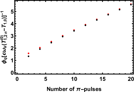
Figure 7: Quantum phase as a function of the number of NCPS. Exact (160) and asymptotic (161) dependences are plotted in black and red, respectively.

IV.1 Phase $\bar{\phi}_{q}$

meaning 7If the recoil frequency is comparable to the inverse pulse duration, then a smooth quantum phase dependence appears not on the distance between the pulses, but on the pulse duration. It arises owing to the fact that the amplitude of the atom in the ground state $\left|g\right\rangle$ on the nonresonant branch of the recoil diagram changes its phase, remaining unchanged in absolute value. The changes are due to the fact that the diagonal elements of the $s-$matrices (76c, 94c, 107c) contain phase factors and also to the fact that the pulse duration depends on the Raman detuning on the nonresonant branch [see Eq. (108)], which, according to Eq. (131), determined by the recoil frequency. In the case of rectangular pulses, we calculated these changes [see phase augmentation in Eqs. (135b, 135d, 135g, 135i)].meaning 7

If all NCPs belong to the same class, $\ell_{\zeta,\beta}=const$, then from Eqs. (91c, 104c, 134, 108, 149b) one could make sure that the phase $\bar{\phi}_{q}$ does not depend on recoil frequency ,

$$\left.\bar{\phi}_{q}\right|_{\ell_{\zeta,\beta}=1}=\dfrac{\pi}{2}\mathop{\displaystyle\sum}_{m=1}^{2n}\left(-1\right)^{m}\left[-\sqrt{4j_{1,m,1}^{2}-1}\right.$$

$$\left.-\sqrt{4j_{2,-m,1}^{2}-1}+\sqrt{4j_{2,m,1}^{2}-1}+\sqrt{4j_{3,-m,1}^{2}-1}\right],$$ (162a)

$$\left.\bar{\phi}_{q}\right|_{\ell_{\zeta,\beta}=2}=\pi\mathop{\displaystyle\sum}_{m=1}^{2n}\left(-1\right)^{m}\left(-j_{1,m,2}-j_{2,-m,2}\right.$$

$$\left.+j_{2,m,2}+j_{3,-m,2}\right),$$ (162b)

$$\left.\bar{\phi}_{q}\right|_{\ell_{\zeta,\beta}=3_{\pm}}=0.$$ (162c)

In these equations, we omitted terms that are multiples of $$2\pi \omega_{k} \ell_{\zeta,\beta}=2 \left\{1.2n\right\} \ell_{1.2n}=3_{\pm}$$. To obtain a phase dependent on , it is necessary that at least one NCP differs from others in the number of rectangular pulses included in it. We have considered the case when for all NCPs , except for the NCP , for which . From Eqs. (90, 91c, 103b, 104c, 149b) one arrives at the result

$$\bar{\phi}_{q}=\left.\bar{\phi}_{q}\right|_{\ell_{\zeta,\beta}=2}+\dfrac{\pi}{2}+\Phi_{\pm}\left(4n\omega_{k}\right),$$ (163a)

$$\Phi_{\pm}\left(\nu\right)=$$

$$-2\arctan\left[\dfrac{2\nu\tau}{\sqrt{\pi^{2}+4\nu^{2}\tau^{2}}}\tan\left(\dfrac{1}{4}\sqrt{\pi^{2}+4\nu^{2}\tau^{2}}\right)\right]$$

$$+\arctan\left(\dfrac{2\nu\tau}{\sqrt{\pi^{2}+4\nu^{2}\tau^{2}}}\tan\dfrac{\tau_{1}}{4\tau}\sqrt{\pi^{2}+4\nu^{2}\tau^{2}}\right)$$

$$+\arctan\dfrac{\mathop{\mathrm{I}m}\left(s_{d1}s_{d2}\right)}{\mathop{\mathrm{R}e}\left(s_{d1}s_{d2}\right)}$$

$$\mp\left[\arccos\dfrac{1}{2}\left|\dfrac{s_{a2}}{s_{a1}s_{d1}}\right|+\arccos\dfrac{\left|s_{a2}\right|\left(\left|s_{a1}\right|^{2}-\left|s_{d1}\right|^{2}\right)}{2\left|s_{a1}s_{d1}s_{d2}\right|}\right]$$ (163b)

The dependencies (163b) are shown in Fig. 8.

Figure 8: Smooth dependence of the phase as a function of the duration of the first rectangular pulse in the NCP $\tau_{1}$ for different values of the parameter $4n\omega_{k}\tau.$

V Gravity phase

meaning 8The main reason for using SLMT is the increase in the gravitational phase of the AI. For this phase, from Eqs. (153, 150a) one obtains.meaning 8

$$\phi_{g}^{\left(0\right)} = \left(\mathbf{k\cdot g}-\alpha\right)\left\{\left(2n+1\right)T^{2}+T\mathop{\displaystyle\sum}_{m=1}^{2n}\left[\left(2n+1-m\right)d_{2,-m+1}+\left(2n+1+m\right)d_{2,m}+2md_{3,-m+1}\right]+\right.$$ (164)

$$+\dfrac{2n+1}{2}\left[\left(\mathop{\displaystyle\sum}_{m=1}^{2n}\left(d_{2,m}+d_{3,-m+1}\right)\right)^{2}-\left(\mathop{\displaystyle\sum}_{m=1}^{2n}\left(d_{1,m}+d_{2,-m+1}\right)\right)^{2}\right]$$

$$+\dfrac{1}{2}\mathop{\displaystyle\sum}_{m=1}^{2n}\left[\left(\mathop{\displaystyle\sum}_{m^{\prime}=1}^{m}d_{1,m^{\prime}}\right)^{2}-\left(\mathop{\displaystyle\sum}_{m^{\prime}=1}^{m}d_{2,-m^{\prime}+1}\right)^{2}-\left(\mathop{\displaystyle\sum}_{m^{\prime}=1}^{m}d_{2,m^{\prime}}\right)^{2}+\left(\mathop{\displaystyle\sum}_{m^{\prime}=1}^{m}d_{3,-m^{\prime}+1}\right)^{2}\right]$$

$$+\left[\mathop{\displaystyle\sum}_{m=1}^{2n}\left(d_{1,m}+d_{2,-m+1}\right)\right]\left[\mathop{\displaystyle\sum}_{m=1}^{2n}\left(\left(2n+1-m\right)d_{2,-m+1}+\left(2n+1+m\right)d_{2,m}+2md_{3,-m+1}\right)\right]$$

$$\left.-\left[\mathop{\displaystyle\sum}_{m=1}^{2n}\left(2n+1-m\right)d_{3,-m+1}\right]\left[\mathop{\displaystyle\sum}_{m^{\prime}=1}^{2n}\left(d_{2,m}+d_{3,-m+1}\right)\right]\right\}.$$

Let us go to the calculation of the correction (150b). In the timing of a given Raman pulse (113), the $\Upsilon_{\zeta,\beta}$ part is the sum of the durations of all preceding pulses, i.e.

$$\Upsilon_{\zeta,m}=\left\{\begin{array}[]{l}\mathop{\displaystyle\sum}_{m^{\prime}=0}^{m-1}\tau\left(\nu,1,m^{\prime},\ell_{1,m^{\prime}}\right),\text{ for }\zeta=1\\ \Upsilon_{\zeta-1,2n}+\tau\left(\nu,\zeta-1,2n,\ell_{\zeta-1,2n}\right)+\mathop{\displaystyle\sum}_{m^{\prime}=-2n}^{m-1}\tau\left(\nu,\zeta,m^{\prime},\ell_{\zeta,m^{\prime}}\right),\text{ for }\zeta>1\end{array}\right.$$ (165)

Here it is convenient to pick out the durations of the main pulses (111), so that

$$\Upsilon_{1,m} = \tau+\Theta_{1,m},$$ (166a)

$$\Upsilon_{2,m} = \left\{\begin{array}[]{c}\tau+\Theta_{2,m},\text{ for }-2n\leq m\leq 0\\ 3\tau+\Theta_{2,m},\text{ for }0<m\leq 2n\end{array}\right.,$$ (166d)

$$\Upsilon_{3,m} = 3\tau+\Theta_{3,m}$$ (166e)

Calculations bring one to the next result

$$\phi_{g}^{\left(1\right)} = \phi_{g\tau}+\phi_{ga},$$ (167a)

$$\phi_{g\tau} = \left(\mathbf{k\cdot g}-\alpha\right)\tau\left\{T\left(4n+2+\dfrac{4}{\pi}\right)+2\mathop{\displaystyle\sum}_{m=1}^{2n}\left[\dfrac{1}{\pi}\left(d_{1,m}+d_{2,-m+1}\right)+\left(\dfrac{1}{\pi}+m\right)\left(d_{2,m}+d_{3,-m+1}\right)\right]\right\},$$ (167b)

$$\phi_{ga} = \left(\mathbf{k\cdot g}-\alpha\right)\left\{-2T_{2,0}^{\left(0\right)}\Theta_{2,0}+T_{3,0}^{\left(0\right)}\Theta_{30}+\mathop{\displaystyle\sum}_{m=1}^{2n}\left[\left(\Theta_{1,m}T_{1,m}^{\left(0\right)}-\Theta_{2,-m}T_{2,-m}^{\left(0\right)}-\Theta_{2,m}T_{2,m}^{\left(0\right)}+\Theta_{3,m}T_{3,-m}^{\left(0\right)}\right)\right.\right.$$ (167c)

$$+\left(\zeta_{m+1}\tau\left(\left(-1\right)^{m}2\xi_{m}\omega_{k},1,m,\ell_{1,m}\right)+\left(-1\right)^{m}\eta_{1}^{\left(\ell_{1,m}\right)}\left(\left(-1\right)^{m}2\xi_{m}\omega_{k}\right)\right)T_{1,m}^{\left(0\right)}$$

$$+\left(\zeta_{m}\tau\left(\left(-1\right)^{m}2\xi_{m}\omega_{k},2,-m,\ell_{2,-m}\right)-\left(-1\right)^{m}\eta_{1}^{\left(\ell_{2,-m}\right)}\left(\left(-1\right)^{m}2\xi_{m}\omega_{k}\right)\right)T_{2,-m}^{\left(0\right)}$$

$$+\left(\zeta_{m+1}\tau\left(\left(-1\right)^{m}2\xi_{m}\omega_{k},2,m,\ell_{2,m}\right)+\left(-1\right)^{m}\eta_{1}^{\left(\ell_{2,m}\right)}\left(2\left(-1\right)^{m}\xi_{m}\omega_{k}\right)\right)T_{2,m}^{\left(0\right)}$$

$$\left.\left.+\left(\zeta_{m}\tau\left(\left(-1\right)^{m}2\xi_{m}\omega_{k},3,-m,\ell_{3,-m}\right)-\left(-1\right)^{m}\eta_{1}^{\left(\ell_{3,-m}\right)}\left(2\left(-1\right)^{m}\xi_{m}\omega_{k}\right)\right)T_{3,-m}^{\left(0\right)}\right]\right\}.$$

In the absence of auxiliary NCPs, at $$n=0$$, one returns to the well-known result i31

$$\phi_{g}=\left(\mathbf{k\cdot g}-\alpha\right)\left[T^{2}+\tau T\left(2+\dfrac{4}{\pi}\right)\right].$$ (168)

meaning 9One should note that the correction (167a), as well as the gravitational phase (164), grows with the increase in the number of NCPs.meaning 9meaning 9

VI Discussion.

The model adopted here, a rectangular pulse of the optical field, is widely used in atomic interferometry and in the theory of atomic clocks i32 . At the same time, we are not aware of the consideration of corrections related to the non-ideal pulse shape. Such corrections arise due to the non-permanent field amplitude inside the pulse and due to the non-zero duration of the forward and backward fronts of the pulse $\tau_{f}$. So instead of one small parameter (1) in the Bragg regime, in our case at least two parameters should be small,

$$\delta\left|\Omega\right|/\left|\Omega\right| \ll 1,$$ (169a)

$$\omega_{k}\tau_{f} \ll 1,$$ (169b)

where $$\delta\left|\Omega\right|$$ is the deviation of the Rabi frequency from a constant value. The article i33 reported that the field intensity was kept constant with an accuracy of 1%, meaning that

$$\delta\left|\Omega\right|/\left|\Omega\right|\sim 5\times 10^{-3}$$ (170)

can be implemented.

In Ref. i34 the front durations were 10ns; with a typical value of $\omega_{k}\sim 10^{5}$s${}^{-\text{1}}$ one has the estimate

$$\omega_{k}\tau_{f}\sim 10^{-3}.$$ (171)

The fact that the small parameters (169) are 40 or 200 times smaller than the parameter (1) allows us to hope that the SLMT option proposed here is feasible.

It should be noted that the durations of the fronts cannot decrease indefinitely, since for the applicability of the adiabatic elimination of the upper level amplitude in Eq. (27), the front duration must be long enough,

$$\Delta\tau_{f}\gg 1.$$ (172)

With a typical value of $\Delta\sim 2\pi\times 1$GHz, $\Delta\tau_{f}\sim 60$. If, however, one will be able to create pulses with picosecond fronts, then in order to use them in atomic interferometry, one must first increase the one-photon detuning $\Delta$ and, accordingly, the field intensity also needs to be increased.

We predict that the MZAI quantum phase will not disappear in our case. It arises due to the phase (46d) in the Schrödinger equation (45), which is also valid in both Bragg (1) and Raman-Nath (4) regimes. Nevertheless, the quantum phase was not observed in either the Bragg regime in i10 or the Raman-Nath regime in i14 . One can explain it by the fact that in those articles the auxiliary pulses were timed out equidistant and in this case the combination of delays between NCPs in Eq. (155) $f_{m}=0$. If one places the NCPs nonequidistant, then our expression (154b) for the quantum phase $\phi_{q}$ can be directly used in the Bragg regime i10 . Here, for example, one can use the nonequidistant NCPs timing shown in Fig. 6.

Our result cannot be used in the Raman-Nath regime, since in this case the atomic momentum in the recoil diagram changes along both branches. An example of such a diagram is shown in i14 . In the Raman-Nath regime, the calculation of the quantum phase must be carried out again. We hope to carry out this calculation in the future.

If the time budget for auxiliary NCPs is comparable to the interrogation time $T$, then the quantum phase (160) at $n\mathbf{\thicksim}\varepsilon\mathbf{\thicksim}1$ is comparable to the maximal expected quantum phase (19b). This is the fundamental difference between our case and the quantum phases considered in Refs. i21 ; i22 ; i23 ; i24 ; i25 , where the quantum phases were only small additions.

Like the gravity phase (6b), the quantum phase grows with an increase in the number of auxiliary NCPs, i.e., with an increase in momentum transfer. However, since the momentum transfer occurs gradually, increasing by $\hbar\mathbf{k}$ under the action of each NCP, the quantum phase grows more slowly than the gravity one in the factor $\ln n$ [see Eq. (161)].

In this work, as in other papers, we assumed that the interrogation time $T$ is the same between the first and second and between the second and third main Raman pulses. The SLMT technique allows us to make these times different, since the resulting Doppler phase can be compensated by Doppler phases during the operation of auxiliary NCPs. With such an opportunity, a quantum phase should also arise. We hope to consider this option in the future.

The quantum phase (160) is linear in time. This is not the only phase linear in time. Another linear phase observed by B. Young i30 is the Ramsey phase (147). In order to extract the quantum phase, we propose to scale all the delay times between pulses into a factor $1+x$,

$$\left\{T_{1,0},d_{\zeta,\beta}\right\}\rightarrow\left(1+x\right)\left\{T_{1,0},d_{\zeta,\beta}\right\}.$$ (173)

If simultaneously one scales the Raman detunings as

$$\delta_{\zeta,\beta}\rightarrow\delta_{\zeta,\beta}/\left(1+x\right),$$ (174)

then the Ramsey phase (147) remains unchanged, only the quantum phase grows linearly in $x$, and the excitation probability $w$ is a periodic function of $x$ with period

$$\Delta x=2\pi\left[\varepsilon\omega_{k}\left(T_{1,2n}^{\left(0\right)}-T_{1,0}\right)\dfrac{2n}{\psi\left(2n+1\right)+\gamma}\right]^{-1}.$$ (175)

To avoid violating the resonance condition (118) during scaling, the parameter $x$ must be small,

$$x\ll\left(\omega_{k}\tau\right)^{-1}.$$ (176)

Since even for $n\mathbf{\thicksim 1}$ and $\varepsilon\mathbf{\thicksim 1}$

$$\Delta x\omega_{k}\tau\sim\dfrac{\tau}{T_{1,2n}^{\left(0\right)}-T_{1,0}}\ll 1,$$ (177)

one can observe many periods of quantum oscillations of the excitation probability without significantly violating the resonance condition.

We predict a new quantum effect, the dependence of the phase on the pulse durations $\tau$ and $\tau_{1}$, the term $\bar{\phi}_{q}$. Unlike the phase linear in $T$ (19b), the term $\bar{\phi}_{q}$ is a non-linear function of $\left\{\tau,\tau_{1}\right\}$. Another difference from the term (19b) is that it is specific only to the variant of SLMT considered here. Neither in the Bragg regime (1) nor in the Raman-Nath regime (4) does the term $\bar{\phi}_{q}$ occur. Its appearance is due to the fact that the Raman frequency detuning on the nonresonant branch of the recoil diagram is proportional to the recoil frequency [see Eq. (131)]. This leads to the fact that in the case of NCPs of type $\ell=1$, the pulse duration at which, owing to Rabi oscillations, the atom is not excited on the nonresonant branch, also depends on $\omega_{k}$, see Eqs. (73, 131). If the NCPs type is $\ell>1$, then the frequency detuning (131) is the atomic coherence nutation frequency in the space between pulses. Therefore, the delay between pulses $\tau_{b}$ also depends on $\omega_{k}$ [see Eqs.(90, 103b, 131)]. Despite that the atoms remain in the ground state on the nonresonant branch of the recoil diagram, the phase of the amplitude of this state changes [see Eqs. (91, 104)] and this change also contributes to the $\bar{\phi}_{q}$ phase. If the rapidly oscillating quantum phase $\phi_{q}$ vanishes at an equidistant location of the NCPs, then the smooth phase $\bar{\phi}_{q}$ also ceases to depend on the recoil frequency if all NCPs are of the same type, see Eqs. (162). It is necessary to use NCPs of different types. In Sec. IV.1 we carried out the calculation in the case when all NCPs are of type $\ell=2$, except for NCP $\left\{1,2n\right\}$, whose type is $\ell_{1,2n}=3$.

Another effect that disappears in the convenient MZAI but appears when additional beam splitters are turned on is the gravitational redshift i31.2 .

Finally, the gravity phase (150a), being quadratic in the Raman pulses’ timing, apart from the main term, the first term in curly brackets in Eq. (164), contains cross terms, combinations of interrogation time and delays $d_{\zeta,\beta}$ between auxiliary NCPs, and terms quadratic in $d_{\zeta,\beta}$. All these terms are pieced together in Eq. (164). From a mathematical point of view, the gravity phase is caused by the phase terms (46d) in the Schrödinger equation (45). Since this equation is valid for any pulse shape $f\left(t\right)$, our result (164) will also be correct in the Bragg regime, under the conditions of the experiment in i10 .

The correction associated with the finite duration of the Raman pulse, on the contrary, depends on the pulse shape i35 . Therefore, the result (167) is only correct for rectangular NCPs.

In this work, we considered only MZAIs. The SLMT method can lead to a significant increase in the AI phase in other cases as well, for the asymmetric MZAI i19 , for atomic two-loop gyroscopes i36 and gravity gradiometers i37 . Calculations of the SLMT technique for these AIs are left for future work. As for the two-loop AIs, as shown in Ref. i22 , the AI response occurs simultaneously with the stimulated echo response, the phase of which is sensitive to gravity acceleration. Two methods have been proposed to resolve this problem, the adjustable momentum transfer i22 and the time-skewed pulse sequence i38 . For atomic gyroscopes, both methods have been implemented in i39 and i38 ; i40 ; i41 . For the atomic gravity gradiometer, only the time-skewed method was used. However, even a small distortion in time led to the appearance of a significant background proportional to the gravity acceleration i37 . No background should occur in the adjustable momentum transfer method.

Appendix A Higher order density harmonics.

The atomic resonant Kapitza-Dirac effect i3' in the field of a standing wave and its analogs lie at the heart of many atomic beam splitters. The momentum transfer to an atom, which is a multiple of $\hbar k$, and the subsequent interference of atomic states with different momenta leads to the appearance of higher harmonics of the atomic density. Density harmonics with a period up to $\lambda/10$, where $\lambda$ is the standing wavelength, have been observed in AI i3.0 . Modifications of the standing wave, i.e., the triangular potential i3.0.1 and the bichromatic standing wave i3.0.2 , have been proposed; moreover, transfer of momentum to an atom $\pm 21\mathbf{\hbar}k$ was observed i3.0.1 . Despite the scattering of atoms at large angles, the scattering indicatrix contains not only the desired states $\pm n\mathbf{\hbar}k$, but also neighboring states …$\left(\pm n-2\right)\hbar\mathbf{k},$ $\left(\pm n-1\right)\hbar\mathbf{k},$ $\left(\pm n+1\right)\hbar\mathbf{k},$ $\left(\pm n+2\right)\hbar\mathbf{k}\ldots$ The asymptotes for $n\mathbf{\gg 1}$ inner tails of this indicatrix were obtained in Refs. i3.0.3 ; i3.0.4 . A complete indicatrix for $3$ types of optical potentials was obtained in Ref. i3.0.5 , where it was also shown that due to neighboring momentum states, the interference pattern with a period of $\lambda/2n$ has a smooth envelope with a period of $\lambda/2$, and because of this, it is obvious that the possibility of using an AI of this type is doubtful, both for precision measurements and for nanolithography. To get rid of this difficulty, one can use i26 the Stern-Gerlach effect i3.0.6 , i.e., an atom scattering in a magnetic field having a uniform gradient. It has been shown that one can obtain an atomic lattice with a period of $100$ nm and a smooth envelope of size $\mathbf{\thicksim}100\mu$, which arises owing to the weak inhomogeneity of the magnetic-field gradient. Another multicolor scheme was proposed in Ref. i3.0.7 , where the beam splitter consisted of tree traveling waves with frequencies and wave vectors $\left\{\Omega,\mathbf{k}\right\},\left\{\Omega+\delta_{1},-\mathbf{k}\right\},\left\{\Omega+\delta_{2},-\mathbf{k}\right\}$. If the frequency detunings are chosen in such a way that $n_{1}\delta_{1}+n_{2}\delta_{2}=0$, then this combination of fields creates an amplitude or phase diffraction grating for atoms with a period $\lambda/2\left(n_{1}+n_{2}\right)$. If the standing wave is replaced by two counterpropagating waves in the lin$\perp$lin configuration, then such a field will be a diffraction phase grating for atoms with a period of $\lambda/4$ i3.0.8 ; i3.0.9 . Note also that the Raman standing wave method was proposed i45 . This technique is now widely known as the double-diffraction scheme i46 . The main point of the method is that two Raman pulses with opposite effective wave vectors $\pm\mathbf{k}$ lead to splitting of the initial momentum state $\left|g,\mathbf{p}\right\rangle$ into two states $\left|e,\mathbf{p}\pm\hbar\mathbf{k}\right\rangle$. Since $k\approx 4\pi/\lambda$, then the interference between the scattered states leads to density modulation, the atomic lattice with a period $\lambda/4$. If one of the Raman pulses has the configuration lin$\parallel$lin and the configuration of the other is lin$\perp$lin, then the Raman standing wave induces an atomic lattice with a period $\lambda/8$ i45 . Scattering potentials with period $\lambda/8$ were calculated for various components of the hyperfine splitting of ${}^{\text{85}}$Rb i47 . One can expect that the Raman standing wave method, in combination with the multicolor technique, produces density harmonics with a period $\lambda/8n.$

References

• (1) B. Y. Dubetskiรฏ, A P. Kazantsev, V. P. Chebotayev, and V. P. Yakovlev, Interference of atoms and formation of atomic spatial arrays in light fields, Pisโ€™ma Zh. Eksp. Teor. Fiz. 39, 531 (1984) [JETP Lett. 39, 649 (1984)].
• (2) Atom Interferometry, edited by P. R. Berman (Academic, Cambridge, 1997)
• (3) Atom Interferometry, Proceedings of the International School of Physics โ€œEnrico Fermi,โ€ย Course CLXXXVIII, Varenna, 2013, edited by G. M. Tino and M. Kasevich (IOS, Amsterdam, 2014).
• (4) R. Geiger, A. Landragin, S. Merlet, F. P. D. Santos, High-accuracy inertial measurements with cold-atom sensors, AVS Quantum Sci. 2, 024702 (2020).
• (5) Q. Zhang, Y. Wang, C. Zhu, Y. Wang, X. Zhang, K. Gao, and W. Zhang, Precision measurements with cold atoms and trapped ions, Chin. Phys. B 29, 093203 (2020).{comment}arXiv:2007.09064 [physics.atom-ph]
• (6) G. M. Tino, Testing gravity with cold atom interferometry: Results and prospects, in Focus on Quantum Sensors for New-Physics Discoveries, edited by M. Safronova and D. Budker, special issue of Quantum Sci. Technol. 6, 024014 (2021).
• (7) A. Bertoldi, P. Bouyer, and B. Canuel, Quantum sensors with matter waves for GW observation, in Handbook of Gravitational Wave Astronomy, edited by C. Bambi, S. Katsanevas, and K. D. Kokkotas (Springer, Singapore, 2021).
• (8) C. Ufrecht, A. Roura, and W. P. Schleich, Bose-Einstein condensates in microgravity and fundamental tests of gravity, arXiv:2107.03709v1 [quant-ph].
• (9) A. Belenchia et al., Quantum physics in space, Physics Reports 951, 1 (2022).
• (10) I. Alonso et al., Cold atoms in space: Community workshop summary and proposed road-map. EPJ Quantum Technol. 9, 30 (2022).
• (11) S. Abend et al., Technology roadmap for cold-atoms based quantum inertial sensor in space, AVS Quantum Sci. 5, 019201 (2023).
• (12) B. Canuel et al., ELGARโ€”A European laboratory for gravitation and atom-interferometric research, Class. Quantum Grav. 37 225017 (2020).
• (13) Ming-Sheng Zhan et al., ZAIGA: Zhaoshan long-baseline atom interferometer gravitation antenna, Int. J. Mod. Phys. D 29, 194005 (2020).
• (14) L. Badurina et al., AION: An atom interferometer observatory and network, J. Cosmol. Astropart. Phys. JCAP05(2020)011
• (15) B. Battelier et al., Exploring the foundations of the universe with space tests of the equivalence principle, Exp. Astron. 51, 1695 (2021).
• (16) Y. A. El-Neaj et al., AEDGE: Atomic experiment for dark matter and gravity exploration in space, EPJ Quantum Technol. 7, 6 (2020).
• (17) G. M. Tino et al., SAGE: A proposal for a space atomic gravity explorer, Eur. Phys. J. D.ย 73, 228 (2019).
• (18) M. Abe et al., Matter-wave Atomic Gradiometer Interferometric Sensor (MAGIS-100), Quantum Sci. Technol. 6, 044003 (2021).
• (19) Rainer Kaltenbaek et al., Quantum technologies in space, Exp. Astron. 51, 1677 (2021).
• (20) H. Ahlers et al., STE-QUEST: Space Time Explorer and Quantum Equivalence principle Space Test, arXiv:2211.15412 [physics.space-ph].
• (21) Q. Beaufils, J. Lefebve, J. G. Baptista, R. Piccon, V. Cambier, L. A. Sidorenkov, C. Fallet, T. Lรฉvรจque, F. P. D. Santos, Rotation related systematic effects in a cold atom interferometer onboard a Nadir pointing satellite, npj Micrograv. 9, 53 (2023).
• (22) S. M. Dickerson, J. M. Hogan, A. Sugarbaker, D. M. S. Johnson, M. A. Kasevich, Multiaxis inertial sensing with long-time point source atom interferometry. Phys. Rev. Lett. 111, 083001 (2013).
• (23) C. D. Panda, M. Tao, J. Egelhoff, M. Ceja, V. Xu, and H. Mรผller, Quantum metrology by one-minute interrogation of a coherent atomic spatial superposition, arXiv:2210.07289 [physics.atom-ph]
• (24) T. Kovachy, S.-W. Chiow, and M. A. Kasevich, Adiabatic-rapid-passage multiphoton Bragg atom optics, Phys. Rev. A 86, 011606(R) (2012).
• (25) J.-N. Kirsten-Siem$\beta$, F. Fitzek, C. Schubert, E.โ€‰M. Rasel, N. Gaaloul, and K. Hammerer, Large-momentum-transfer atom interferometers with $\mu$rad -accuracy using Bragg diffraction, Phys. Rev. Lett. 131, 033602 (2023).
• (26) P. Cladรฉ, S. Guellati-Khรฉlifa, F. Nez, and F. Biraben, Large momentum beam splitter using Bloch oscillations, Phys. Rev. Lett. 102, 240402 (2009).
• (27) M. H. Goerz, M. A. Kasevich and V. S. Malinovsky, Robust optimized pulse schemes for atomic fountain interferometry, Atoms 11, 36 (2023).
• (28) D. S. Weiss, B. C. Young, and S. Chu, Precision measurement of the photon recoil of an atom using atomic interferometry, Phys. Rev. Lett. 70, 2706 (1993).
• (29) A. P. Kolโ€™chenko, S. G. Rautian, and R. I. Sokolovskii, Interaction of an atom with a strong electromagnetic field with the recoil effect taken into consideration, Zh. Eksp. Teor. Fiz. 55, 1864 (1968) [JETP 28, 986 (1969)].
• (30) T. Kovachy, P. Asenbaum, C. Overstreet, C. A. Donnelly, S. M. Dickerson, A. Sugarbaker, J. M. Hogan, and M. A. Kasevich, Quantum superposition at the half-metre scale, Nature 528, 530 (2015).
• (31) B. Plotkin-Swing, D. Gochnauer, K. E. McAlpine, E. S. Cooper, A. O. Jamison, and S. Gupta, Three-path atom interferometry with large momentum separation, Phys. Rev. Lett. 121, 133201 (2018).
• (32) T. Kovachy, J. M. Hogan, D. M. S. Johnson, and M. A. Kasevich, Optical lattices as waveguides and beam splitters for atom interferometry: An analytical treatment and proposal of applications, Phys. Rev. A 82, 013638 (2010).
• (33) J. Rudolph, T. Wilkason, M. Nantel, H. Swan, C. M. Holland, Y. Jiang, B. E. Garber, S. P. Carman, and J. M. Hogan, Large momentum transfer clock atom interferometry on the 689 nm intercombination line of strontium, Phys. Rev. Lett. 124, 083604 (2020).
• (34) M Gebbe, J.-N. Siem$\beta$ , M. Gersemann, H. Mรผntinga , S. Herrmann, C. Lรคmmerzahl1, H.Ahlers, N. Gaaloul, C. Schubert, K. Hammerer, S. Abend, and E. M. Rasel, Twin-lattice atom interferometry. Nat. Commun. 12, 2544 (2021).
• (35) R. H. Parker, C. Yu, W. Zhong, B. Estey, and H. Mรผller, Measurement of the fine-structure constant as a test of the Standard Model, Science 360, 191 (2018).
• (36) E. Peik, M. B. Dahan, I. Bouchoule, Y. Castin, and C. Salomon, Bloch oscillations of atoms, adiabatic rapid passage, and monokinetic atomic beams, Phys. Rev. A 55, 2989 (1997).
• (37) L. Morel, Z. Yao, P. Cladรฉ, and S. Guellati-Khรฉlifa, Determination of the fine-structure constant with an accuracy of 81 parts per trillion, Nature 588, 61 (2020).
• (38) M. A. Kasevich and B. Dubetsky, Kinematic sensors employing atom interferometer phases, US Patent 7,317,184 (8 January 2008).
• (39) B. Dubetsky, Local positioning system as a classic alternative to atomic navigation, The Journal of Navigation 75, 273 (2022).
• (40) M. Kasevich and S. Chu, Atomic interferometry using stimulated Raman transitions, Phys. Rev. Lett. 67, 181 (1991).
• (41) F. Riehle, Th. Kisters, A. Witte, J. Helmcke, and Ch. J. Bordรฉ, Optical Ramsey spectroscopy in a rotating frame: Sagnac effect in a matter-wave interferometer, Phys. Rev. Lett. 67, 177 (1991).
• (42) E. M. Rasel, M. K. Oberthaler, H. Batelaan, J. Schmiedmayer, and A. Zeilinger, Atom wave interferometry with diffraction gratings of light, Phys. Rev. Lett. 75, 2633 (1995).
• (43) S. B. Cahn, A. Kumarakrishnan, U. Shim, T. Sleator, P. R. Berman, and B. Dubetsky, Time-domain de Broglie wave interferometry, Phys. Rev. Lett. 79, 784 (1997).
• (44) V. P. Chebotayev, B. Y. Dubetsky, A. P. Kazantsev, and V. P. Yakovlev, Interference of atoms in separated optical fields in: Special issue on โ€The Mechanical Effects of Lightโ€ ed. by P. Meystre, S. Stenholm, J. Opt. Soc. Am. B,ย 2, 1791 (1985).
• (45) C. J. Bordรฉ, Atomic interferometry with internal state labeling, Phys. Lett. 140, 10 (1989).
• (46) S. Hartmann, J. Jenewein, E. Giese, S. Abend, A. Roura, E. M. Rasel, and W. P. Schleich, Regimes of atomic diffraction: Raman versus Bragg diffraction in retroreflective geometries, Phys. Rev. A 101, 053610 (2020).
• (47) B. Dubetsky and P. R. Berman, $\lambda/4$, $\lambda/8$ and higher order atom gratings via Raman transitions, Laser Phys. 12, 1161 (2002).
• (48) T. Lรฉvรจque, A. Gauguet, F. Michaud, F. P. D. Santos, and A. Landragin, Enhancing the area of a Raman atom interferometer using a versatile double-diffraction technique, Phys. Rev. Lett. 103, 080405 (2009).
• (49) E. Giese, A. Roura, G. Tackmann, E. M. Rasel, and W. P. Schleich, Double Bragg diffraction: A tool for atom optics, Phys. Rev. A 88, 053608 (2013).
• (50) S. Hartmann, J. Jenewein, S. Abend, A. Roura, and E. Giese, Atomic Raman scattering: Third-order diffraction in a double geometry, Phys. Rev. A 102, 063326 (2020).
• (51) M. Chiarotti, J. N. Tinsley, S. Bandarupally, S. Manzoor, M. Sacco, L. Salvi, and N. Poli, Practical limits for large-momentum-transfer clock atom interferometers, PRX Quantum 3, 030348 (2022).
• (52) P. Asenbaum, C. Overstreet, M. Kim, J. Curti, and M. A. Kasevich, Atom-interferometric test of the equivalence principle at the $10^{-12}$ level, Phys. Rev. Lett. 125, 191101 (2020).
• (53) S.-W. Chiow, T. Kovachy, H.-C. Chien, and M. A. Kasevich, 102$\hbar$k large area atom interferometers, Phys. Rev. Lett. 107, 130403 (2011).
• (54) I. I. Rabi, Space quantization in a gyrating magnetic field Phys. Rev. 51, 652 (1937).
• (55) M. H. Levitt and R. Freeman, NMR population inversion using a composite pulse, Journal of Magnetic Resonance 33, 473-476 (1979).
• (56) J. Saywell, M. Carey, M. Belal, I. Kuprov and T. Freegarde, Optimal control of Raman pulse sequences for atom interferometry, J. Phys. B 53, 085006 (2020).
• (57) B. Dubetsky, Asymmetric Mach-Zehnder atom interferometers, arXiv:1710.00020v6 [physics.atom-ph].
• (58) The expression (6b) at $n=0$ was first derived for phases of the neutron interferometer, see Eq. (4.8) in the article by D. M. Greenberger and A. W. Overhauser, Coherence effects in neutron diffraction and gravity experiments, Rev. Mod. Phys.ย 51, 43 (1979).
• (59) T. Sleator, P. R. Berman, and B. Dubetsky, High precision atom interferometry in a microgravity environment, arXiv:physics/9905047 [physics.atom-ph].
• (60) B. Dubetsky and P. R. Berman, Ground-state Ramsey fringes, Phys. Rev. A 56, R1091 (1997).
• (61) B. Dubetsky and M. A. Kasevich, Atom interferometer as a selective sensor of rotation or gravity, Phys. Rev. A 74, 023615 (2006).
• (62) K. Bongs, R. Launay, and M. A. Kasevich, High-order inertial phase shifts for time-domain atom interferometers, Appl. Phys. B 84, 599 (2006).
• (63) B. Dubetsky, S. B. Libby, and P. Berman, Atom interferometry in the presence of an external test mass, Atoms 4, 14 (2016).
• (64) P. Asenbaum, C. Overstreet, T. Kovachy, D. D. Brown, J. M. Hogan, and M. A. Kasevich, Phase shift in an atom interferometer due to spacetime curvature across its wave function, Phys. Rev. Lett. 118, 183602 (2017).
• (65) B. Dubetsky and G. Raithel, Nanometer scale period sinusoidal atom gratings produced by a Stern-Gerlach beam splitter, arXiv:physics/0206029 [physics.atom-ph].
• (66) The inequality (25b) means that during the time $\Delta^{-1}$ one can neglect the changes in the phase of the wave function associated with the Raman frequency detuning $\tilde{\delta}$, with the Doppler shift (18b) and the change in this shift due to the acceleration of the atom |๐ชiโ‹…๐ |โ€‹Tโ‹…subscript๐ช๐‘–๐ ๐‘‡\left|\mathbf{q}_{i}\cdot\mathbf{g}\right|T, with the recoil frequency (2), with characteristic times of change in the amplitude and phase of the fields $\tau_{f}$ and $\dot{\phi}^{-1}$. Under these conditions, one can eliminate the first term on the right-hand side of Eq. (24c) and then, using integration by parts, arrive at the expression (27) for the level $\left|o\right\rangle$ amplitude.
• (67) J. M. McGuirk, G. T. Foster, J. B. Fixler, M. J. Snadden, and M. A. Kasevich, Sensitive absolute-gravity gradiometry using atom interferometry, Phys. Rev. A 65, 033608 (2002).
• (68) A. Louchet-Chauvet, T. Farah, Q. Bodart, A. Clairon, A. Landragin, S. Merlet and F. P. D. Santos, The influence of transverse motion within an atomic gravimeter, New J. Phys. 13 065025 (2011).
• (69) Another possibility here is to place detunings $\Delta$ between sublevels of the hyperfine structure of the state $o$, so that the contributions to the ac-Stark shift from different sublevels cancel each other.
• (70) L. D. Landau andย E. M. Lishitz, Quantum Mehanics: Non-relativistic Theory (Pergamon, Oxford,1989), translated by J. B. Sykes and J. S. Bell from the fourth edition, Moscow Nauka 1989, p. 205, problem 1.
• (71) A. Peters, High precision gravity measurements using atom interferometry, Ph. D. thesis, Stanford University, 1998.
• (72) C. Antoine, Matter wave beam splitters in gravito-inertial and trapping potentials: Generalized ttt scheme for atom interferometry, Appl. Phys. B 84, 585 (2006).
• (73) A. Bertoldi, F. Minardi, and M. Prevedelli, Phase shift in atom interferometers: Corrections for nonquadratic potentials and finite-duration laser pulses, Phys. Rev. A 99, 033619 (2019).
• (74) N. F. Ramsey, A New Molecular Beam Resonance Method, Phys. Rev. 76, 996 (1949).
• (75) V. I. Yudin, A. V. Taichenachev, C. W. Oates, Z. W. Barber, N. D. Lemke, A. D. Ludlow, U. Sterr, C. Lisdat, and F. Riehle, Hyper-Ramsey spectroscopy of optical clock transitions, Phys. Rev. A 82, 011804(R) (2010).
• (76) N. Huntemann, B. Lipphardt, M. Okhapkin, C. Tamm, E. Peik, A. V. Taichenachev, and V. I. Yudin, Generalized Ramsey Excitation Scheme with Suppressed Light Shift, Phys. Rev. Lett. 109, 213002 (2012).
• (77) A. C. Carew, Apparatus for inertial sensing with cold atoms, Ph. D. thesis, York University, 2018.
• (78) B. C. Young, Private communications, 2010.
• (79) F. Di Pumpo, C. Ufrecht, A. Friedrich, E. Giese, W. P. Schleich, and W. G. Unruh, Gravitational redshift tests with atomic clocks and atom interferometers, PRX Quantum 2, 040333 (2021).
• (80) B. Fang, N. Mielec, D. Savoie, M. Altorio, A. Landragin, and R. Geiger, Improving the phase response of an atom interferometer by means of temporal pulse shaping, New J. Phys. 20, 023020 (2017).
• (81) J. F. Clauser, Ultra-high sensitivity accelerometers and gyroscopes using neutral atom matter-wave interferometry in Proceedings of the International Workshop on Matter Wave Interferometry in the Light of Schrodingerโ€™s Wave Mechanics, G. Badurek, H. Rauch and A. Zeilinger editors, 1987, Physica B+C 151, 262 (1988).
• (82) I. Perrin, M. Cadoret, Y. Bidel, N. Zahzam, C. Blanchard, and A. Bresson, Proof-of-principle demonstration of vertical gravity gradient measurement using a single proof mass double-loop atom interferometer, Phys. Rev. A 99, 013601 (2019).
• (83) J. K. Stockton, K. Takase, and M. A. Kasevich, Absolute geodetic rotation measurement using atom interferometry, Phys. Rev. Lett. 107, 133001 (2011).
• (84) L.โ€‰A. Sidorenkov, R. Gautier, M. Altorio, R. Geiger, and A. Landragin, Tailoring multi-loop atom interferometers with adjustable momentum transfer, Phys. Rev. Lett. 125, 213201 (2020).
• (85) I. Dutta, D. Savoie, B. Fang, B. Venon, C. L. Garrido Alzar, R. Geiger, and A. Landragin, Continuous cold-atom inertial sensor with 1 nrad/ sec rotation stability, Phys. Rev. Lett. 116, 183003 (2016).
• (86) R. Gautier, M. Guessoum, L. A. Sidorenkov, Q. Bouton, A. Landragin, and R. Geiger, Accurate measurement of the Sagnac effect for matter waves, Science Advances, 8, eabn8009 (2022).
• (87) A. P. Kazantsev and G. I. Surdutovich, The Kapitza-Dirac effect for atoms in a strong resonant field, Pisโ€™ma Zh. Eksp. Teor. Fiz. 21, 346 (1975) [JETP Lett. 21, 158 (1975)].
• (88) A. Turlapov, A. Tonyushkin, and T. Sleator, Talbot-Lau effect for atomic de Broglie waves manipulated with light, Phys. Rev. A 71, 043612 (2005).
• (89) T. Pfau, C. Kurtsiefer, C. S. Adams, M. Sigel, and J. Mlynek, Magneto-optical beam splitter for atoms, Phys. Rev. Lett. 71, 3427 (1993).
• (90) R. Grimm, J. Sรถding, and Yu. B. Ovchinnikov, Coherent beam splitter for atoms based on a bichromatic standing light wave, Opt. Lett. 19, 658 (1994).
• (91) A. P. Kazantsev, G. I. Surdutovich and V. P. Yakovlev, On the quantum theory of resonance scattering of atoms by light, Pisโ€™ma Zh. Eksp. Teor. Fiz. 31, 542 (1980) [JETP Lett. 31, 509 (1980)].
• (92) P. L. Gould and D. E. Pritchard, Atoms interacting with standing light waves: Diffraction, diffusion and rectification, in Coherent and Collective Interactions of Particles and Radiation Beams, Proceedings of the International School of Physics โ€œEnrico Fermi,โ€ย Course CXXXI, Varenna, 1995, edited by A. Aspect,W. Barletta, and R. Bonifacio (IOS, Amsterdam, 1996), Vol. 131, p. 443.
• (93) B. Dubetsky and P. R. Berman, Atom gratings produced by large-angle atom beam splitters, Phys. Rev. A 64, 063612 (2001).
• (94) W. Gerlach, O. Stern, Der experimentelle nachweis des magnetischen moments des silberatoms. Z. Physik 8, 110 (1922).
• (95) P. R. Berman, B. Dubetsky, and J. L. Cohen, High-resolution amplitude and phase gratings in atom optics, Phys. Rev. A 58, 4801 (1998).
• (96) R. Gupta, J. J. McClelland, P. Marte, and R. J. Celotta, Raman-induced avoided crossings in adiabatic optical potentials: Observation of $\lambda/8$ spatial frequency in the distribution of atoms, Phys. Rev. Lett. 76, 4689 (1996).
• (97) P. S. Jessen and I. H. Deutsch, Optical Lattices, Adv. At. Mol. Opt. Phys. 37, 95 (1996).
• (98) B. Dubetsky and P. R. Berman, $\lambda/8$-period optical potentials, Phys. Rev. A 66, 045402 (2002).