Array-Informed Waveform Design for Active Sensing: Diversity, Redundancy, and Identifiability

Abstract

This paper investigates the combined role of transmit waveforms and (sparse) sensor array geometries in active sensing multiple-input multiple-output (MIMO) systems. Specifically, we consider the fundamental identifiability problem of uniquely recovering the unknown scatterer angles and coefficients from noiseless spatio-temporal measurements. Assuming a sparse scene, identifiability is determined by the Kruskal rank of a highly structured sensing matrix, which depends on both the transmitted waveforms and the array configuration. We derive necessary and sufficient conditions that the array geometry and transmit waveforms need to satisfy for the Kruskal rank—and hence identifiability—to be maximized. Moreover, we propose waveform designs that maximize identifiability for common array configurations. We also provide novel insights on the interaction between the waveforms and array geometry. A key observation is that waveforms should be matched to the pattern of redundant transmit-receive sensor pairs. Redundant array configurations are commonly employed to increase noise resilience, robustify against sensor failures, and improve beamforming capabilities. Our analysis also clearly shows that a redundant array is capable of achieving its maximum identifiability using fewer linearly independent waveforms than transmitters. This has the benefit of lowering hardware costs and transmission time. We illustrate our findings using multiple examples with unit-modulus waveforms, which are often preferred in practice.

I Introduction

Active sensing is distinguished from passive sensing by the ability of designing the transmitted waveforms. Prominent active sensing applications include radar, sonar, and medical ultrasound, as well as autonomous sensing [1, 2], automotive radar [3, 4, 5, 2, 6, 7], and emerging wireless systems integrating communications and sensing [8, 9, 10, 11]. The transmitted waveforms crucially impact the beamforming capability, signal-to-noise-ratio (SNR), probability of target detection, spatio-temporal (angle-range-Doppler) resolution, and number of identifiable scatterers or signal sources, to name a few. Consequently, waveform design is an important topic with a rich literature—see, e.g., [12, 13, 14, 15] and references therein.

The role of waveform design is pronounced in MIMO sensing systems deploying arrays of transmit and receive sensors, where waveform diversity [16, 17] can be leveraged by, for instance, launching independent waveforms from each transmit sensor. Adjusting the cross-correlations between the transmitted signals, and thus the number of linearly independent waveforms—henceforth referred to as the waveform rank (WR)—enables flexibly trading-off between coherent combining gain on transmit and illuminating a wide field of view. A low WR has the benefit of requiring fewer expensive radio-frequency-to-intermediate-frequency (RF-IF) front ends at the transmitter and fewer receive filters, if matched/mismatched filtering is employed. Reducing the WR may also be desirable when deploying a large number of sensors or when operating in a rapidly changing environment, since maintaining linear independence between an increasing number of waveforms entails longer transmission times. Hence, reduced WR may be appealing in highly dynamical automotive radar scenarios, or joint communication and sensing (JCS) applications where a single base station can have hundreds of antennas or more.

A notable example of a MIMO sensing system is colocated MIMO radar [19, 20], which can increase spatial resolution and the number of identifiable scatterers by virtue of the virtual array or sum co-array consisting of the pairwise sums of transmit and receive antenna positions. A MIMO radar is able to access the full virtual array by isolating the (backscatter) channels between each transmit-receive antenna pair. This is conventionally achieved by transmitting waveforms that are orthogonal in space, time, frequency, or polarization [16], and by employing matched filtering at the receiver. Although it may seem that orthogonal (or more generally, linearly independent) waveforms are necessary for realizing the sum coarray, it is important to recognize that the sum coarray actually arises irrespective of the WR and (linear) receive processing. For example, single-input single-output (SIMO) imaging systems can compensate for the lack of waveform diversity by temporal multiplexing [21, 22, 23]. The extent to which a MIMO system can leverage the co-array nevertheless depends on both the WR and array redundancy. Redundant array geometries are relevant in a multitude of applications, such as JCS or automotive radar, where the physical area for placing sensors is limited and one may afford to employ more sensors than is strictly necessary to achieve a desired co-array. Redundant arrays can also improve beamforming capability and robustness to noise compared to arrays with the same aperture but fewer physical sensors.

Past works have not fully investigated the possibility of leveraging the co-array when transmitting linearly dependent waveforms. Instead, major emphasis has been placed on the (no less important) task of transmit beamforming [24, 25, 26, 27, 28]. An exception is [23], which investigated the spatio-temporal trade-off between array redundancy and the number of transmissions required to synthesize a desired transmit-receive beampattern in SIMO imaging. Related trade-offs have also been investigated in the context of passive direction finding [29, 30]. Another relevant recent work [31] considered leveraging the virtual array for JCS by allocating orthogonal sensing waveforms to a subset of the transmit sensors, while transmitting a communication waveform from the remaining sensors. However, which subsets of sensors should be used for sensing has not been investigated in detail. More generally, the relationship between WR, array redundancy and sensing performance is incompletely addressed in the literature, and fundamental questions remain unanswered regarding the impact of the array geometry on waveform design. This paper revisits the classical topic of waveform design from the perspective of the array geometry. We adopt the design criterion of maximizing identifiability given an array geometry, and address questions such as: Can waveform matrices of equal rank yield different identifiability conditions? Could identifiability differ for identical transmit beampatterns? We will show that the answer to both of these questions is, perhaps surprisingly, yes.

Naturally, identifiability is an established topic in array processing. Although early contributions mainly focused on passive sensing [32, 33, 34, 35], more recent works also consider the MIMO active sensing setting [36, 37, 38, 39, 40]. However, most of these works either assume full WR (typically, orthogonal waveforms), or lack rigorous identifiability conditions that also yield insight into the interaction between the waveform and array geometry. This paper attempts to bridge this gap by characterizing the Kruskal rank of the so-called spatio-temporal sensing matrix—a fundamental object in active sensing systems. Our analysis is rigorous, yet simple, readily interpretable, and of practical interest in diverse applications, including automotive radar, autonomous sensing, and JCS.

I-A Problem formulation

We consider the following noiseless on-grid sparse recovery problem: Given measurement vector $\bm{y}\!=\!\bm{B}\bm{x}\!\in\!\mathbb{C}^{m}$ and sensing matrix $\bm{B}\!\in\!\mathbb{C}^{m\times V}$, find the unknown $K$-sparse ground truth vector $\bm{x}\!\in\!\mathbb{C}^{V}$ by solving the following optimization problem:

$$\underset{\bm{z}\in\mathbb{C}^{V}}{\text{minimize}}\ \|\bm{z}\|_{0}\ \text{subject to}\ \bm{y}=\bm{B}\bm{z}.$$ (P0)

We are primarily interested in the support of $\bm{x}$ (typically $K\ll V$), which in sensing applications usually encodes information about the positions or velocities of scatterers/emitters. Our focus is on the fundamental identifiability question “when can $\bm{x}$ be uniquely recovered from (P0)?” The well-known answer is given by the Kruskal rank [41] of $\bm{B}$.

Definition 1 (Kruskal rank).

The Kruskal rank of matrix $\bm{B}$, denoted $\operatorname{k-rank}(\bm{B})$, is the largest integer $r$ such that every $r$ columns of $\bm{B}$ are linearly independent.

The Kruskal rank of $\bm{B}$ yields a necessary and sufficient condition for (P0) to have a unique solution [42, 43].

Theorem 1 (Identifiability [43, Theorem 1]).

Given $\bm{y}\!=\!\bm{B}\bm{x}$, where $\|\bm{x}\|_{0}\!=\!K$, solving (P0) uniquely recovers $\bm{x}$ if and only if $\operatorname{k-rank}(\bm{B})\!\geq\!2K$.

The goal of this paper is to design $\bm{B}$ such that $\operatorname{k-rank}(\bm{B})$ is maximized. This is a nontrivial task because in active sensing, $\bm{B}$ is highly structured and determined by both the transmitted waveforms and the array geometry. In particular, $\bm{B}$ has the following spatio-temporal structure:

$$\bm{B} \triangleq(\bm{S}\bm{A}_{\operatorname{t}})\operatorname{\odot}\bm{A}_{\operatorname{r}}=(\bm{S}\operatorname{\otimes}\bm{I}_{N_{\operatorname{r}}})(\bm{A}_{\operatorname{t}}\operatorname{\odot}\bm{A}_{\operatorname{r}}).$$ (1)

Here, $\operatorname{\otimes}$ and $\operatorname{\odot}$ denote the Kronecker and Khatri-Rao (columnwise Kronecker) products, respectively. A derivation of (1) and further details are deferred to Sections II and III.

The key quantities in (1) are the so-called transmit and receive array manifold matrices $\bm{A}_{\operatorname{t}}\in\mathbb{C}^{N_{\operatorname{t}}\times V}$ and $\bm{A}_{\operatorname{r}}\in\mathbb{C}^{N_{\operatorname{r}}\times V}$, as well as the spatio-temporal waveform matrix $\bm{S}\in\mathbb{C}^{T\times N_{\operatorname{t}}}$. Matrices $\bm{A}_{\operatorname{t}}$ and $\bm{A}_{\operatorname{r}}$, which are determined by the employed transmit and receive array configurations, have Fourier structure. As a consequence, the effective transmit-receive array manifold $\bm{A}_{\operatorname{t}}\operatorname{\odot}\bm{A}_{\operatorname{r}}$ gives rise to an additive (virtual array) structure called the sum co-array (see Section III). We assume that $\bm{A}_{\operatorname{t}}$ and $\bm{A}_{\operatorname{r}}$ are fixed, but $\bm{S}$ can be freely chosen, subject to a rank constraint $\operatorname{rank}(\bm{S})=N_{s}$, where $1\leq N_{s}\leq N_{\operatorname{t}}$. The value of $N_{s}$ is typically constrained by SNR, hardware, or computational considerations in practice.

I-B Contributions

This paper investigates the impact of the array geometry and transmit waveforms on fundamental identifiability conditions in active sensing. Our analysis departs from past works by characterizing the Kruskal rank of sensing matrix $\bm{B}$ in (1) for various waveform rank regimes (values of $N_{s}$), highlighting the role of both properties of the transmit waveforms ($\bm{S}$) and joint transmit-receive array geometry ($\bm{A}_{\operatorname{t}}\operatorname{\odot}\bm{A}_{\operatorname{r}}$).

Our main contributions are as follows.

1. Minimum waveform rank: We show that array geometries containing redundancy can identify the maximum number of scatterers (upper bounded by the size of the sum co-array), and hence fully utilize the virtual array, without employing a full rank waveform matrix. This enables redundant arrays to use their spatial resources more efficiently. For example, beamforming may be used to improve SNR without sacrificing identifiability.

2. Identifiability conditions: We derive necessary and sufficient conditions for maximizing the Kruskal rank of the sensing matrix for any given waveform rank $N_{s}$. These conditions highlight the varying roles played by the array geometry and waveforms in different waveform rank regimes. In general, maximizing identifiability for a given array geometry requires aligning the transmitted waveforms with the subspace determined by the mapping between physical and virtual sensor positions. Specifically, the intersection between the range space of this so-called “redundancy pattern” and the null space of a waveform-dependent matrix should be minimized.

3. Achievability of optimal identifiability: We provide waveform designs (of different WR) yielding sensing matrices that attain maximal Kruskal rank for the given value of $N_{s}$. Interestingly, identifiability is not determined by $N_{s}$ alone, and two waveform matrices of equal rank can lead to sensing matrices with different Kruskal rank. The considered waveforms are matched to a general array structure subsuming the canonical uniform array and nonredundant nested (“MIMO”) array geometries as special cases.

Our results establish that achieving maximal identifiability generally necessitates “matching” the transmit waveforms to the effective transmit-receive array geometry. The proposed “array-informed” approach to waveform design provides a novel, more nuanced perspective on MIMO radar, impacting timely applications including automotive radar and JCS [2].

I-C Organization

The paper is organized as follows. Section II introduces the signal model, and Section III reviews the fundamental role of the sum co-array in active sensing. Section IV formalizes the notions of the maximal Kruskal rank of the sensing matrix and the minimal redundancy-limited waveform rank. Section V derives necessary and sufficient conditions that the waveform matrix should satisfy to maximize the Kruskal rank (given an array geometry). Section VI shows the existence of waveform designs achieving maximal Kruskal rank for a family of array geometries with varying redundancy. Section VII provides illustrative examples demonstrating how matching or failing to match the waveform to the array geometry yields optimal or sub-optimal Kruskal rank, even for the same waveform rank. Section VIII concludes the paper. Basic properties of the Kruskal rank are reviewed in Appendix A.

Notation: We denote matrices by boldface uppercase, e.g, $\bm{A}$; vectors by boldface lowercase, $\bm{a}$; and scalars by unbolded letters, $A,a$. The $(n,m)$th element of matrices $\bm{A}$ and $\bm{A}_{i}$ is $A_{nm}$ and $[\bm{A}_{i}]_{nm}$, respectively. Furthermore, $\bm{A}^{\operatorname{\top}}$, $\bm{A}^{\operatorname{H}}$, and $\bm{A}^{\ast}$ denote transpose, Hermitian transpose, and complex conjugation. The $N\times N$ identity matrix is denoted by $\bm{I}_{N}$, and the standard unit vector, consisting of zeros except for the $i$th entry (which is unity) by $\bm{e}_{i}$ (dimension specified separately). Moreover, $\text{vec}(\cdot)$ stacks the columns of its matrix argument into a column vector, whereas $\text{diag}(\cdot)$ constructs a diagonal matrix of its vector argument. The indicator function is denoted by $\mathbbm{1}(\cdot)$, the ceiling function by $\lceil\cdot\rceil$, and the number of nonzero entries in $N$-dimensional vector $\bm{x}$ by $\|\bm{x}\|_{0}\triangleq\sum_{i=1}^{V}\mathbbm{1}(x_{i}\neq 0)$. Additionally, $\mathcal{R}(\cdot)$, $\mathcal{N}(\cdot)$, and $\dim(\cdot)$ denote the range space, null space, and dimension, respectively. The Kronecker and Khatri-Rao (columnwise Kronecker) products are denoted by $\operatorname{\otimes}$ and $\operatorname{\odot}$, respectively. Sets are denoted by bold blackboard letters, such as $\mathbb{A}$. The subset of integers between $a,b\in\mathbb{R}$ is denoted $[a\operatorname{:}b]\triangleq\{c\in\mathbb{Z}\ |\ a\leq c\leq b;a,b\in\mathbb{R}\}$, and the sum set of $\mathbb{A}$ and $\mathbb{B}$ is defined as $\mathbb{A}+\mathbb{B}\triangleq\{a+b\ |\ a\in\mathbb{A},b\in\mathbb{B}\}$. Finally, subscripts ‘${\operatorname{t}}$’, ‘${\operatorname{r}}$’, and ‘${\operatorname{\xi}}$’ denote “transmitter”, “receiver”, and “transmitter or receiver”, respectively.

II Active sensing model and waveform rank

Fig. 1 illustrates the considered MIMO active sensing system. The transmit (Tx) array illuminates a collection of $K$ far field point targets, whose backscattered signals are measured by the receive (Rx) array. The Tx and Rx arrays are one-dimensional, colinear, and colocated. This means that the angular directions of the scatterers relative to both the Tx and Rx array are equal. The sensors of the two arrays need not be shared and the array geometries can be sparse. The number of Tx and Rx sensors is $N_{\operatorname{t}}$ and $N_{\operatorname{r}}$, respectively.

For simplicity, we restrict our analysis to the angular domain (considering a fixed range-Doppler bin). Our model is noiseless, since we focus on the fundamental identifiability conditions of the scatterer angles and scattering coefficients.

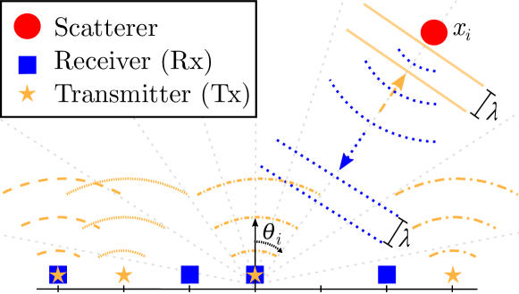
Figure 1: Active sensing signal model. A linear Tx array with $N_{\operatorname{t}}$ sensors uses $N_{s}\leq N_{\operatorname{t}}$ linearly independent waveforms (modulated by a carrier with wavelength $\lambda$) to illuminate $K$ far field point scatterers. The scatterers lie on angular grid of size $V\gg K$, and the scattering coefficients are denoted by $\{x_{i}\}_{i=1}^{V}$, where $K$ of the $x_{i}$’s are nonzero. The backscattered radiation then impinges on a linear Rx array with $N_{\operatorname{r}}$ sensors, colocated with the Tx array.

II-A Received signal model

We consider a sparse on-grid model of $V$ potential scatterer angles $\theta_{i}\in[-\tfrac{\pi}{2},\tfrac{\pi}{2})$, where $\theta_{i}\neq\theta_{k}\ \forall i\neq k\in[1\operatorname{:}V]$. Here, $V$ can be arbitrarily large (but finite) and the grid points can be arbitrarily chosen as long as they are distinct. The discrete-time $N_{\operatorname{r}}\!\times\!T$ Rx signal matrix in absence of noise is [44, 45]

$$\bm{Y}=\bm{A}_{\operatorname{r}}\operatorname{diag}(\bm{x})\bm{A}_{\operatorname{t}}^{\operatorname{\top}}\bm{S}^{\operatorname{\top}},$$ (2)

where $\bm{x}\in\mathbb{C}^{V}$ is an unknown deterministic sparse scattering coefficient vector with $K\ll V$ nonzero entries, and $\bm{S}\in\mathbb{C}^{T\times N_{\operatorname{t}}}$ is a known deterministic spatio-temporal Tx waveform matrix whose columns represent the signals launched from the respective Tx sensors. Here, $T\in\mathbb{N}_{+}$ is the waveform length (in samples), or alternatively, the number of chips or channel uses (block length). The phase shifts incurred by the narrowband radiation transmitted/received by the Tx/Rx array is modeled by the Tx/Rx manifold matrix $\bm{A}_{\operatorname{\xi}}\in\mathbb{C}^{N_{\operatorname{\xi}}\times V}$, where subscript ‘${\operatorname{\xi}}$’ is shorthand for the transmitter ‘${\operatorname{t}}$’ or receiver ‘${\operatorname{r}}$’. Assuming omnidirectional and ideal sensors separated by multiples of half a wavelength $\tfrac{\lambda}{2}$, the $(n,i)$th entry of $\bm{A}_{\operatorname{\xi}}$ is

$$[\bm{A}_{\operatorname{\xi}}]_{n,i}=\exp(j\pi d_{\operatorname{\xi}}[n]\sin\theta_{i}).$$ (3)

Here, $d_{\operatorname{\xi}}[n]\!\in\!\mathbb{Z}$ is the $n$th Tx/Rx sensor position in units of $\tfrac{\lambda}{2}$.

Vectorizing $\bm{Y}$ yields the $N_{\operatorname{r}}T$-dimensional Rx vector

$$\bm{y}\triangleq\operatorname{vec}(\bm{Y})=\bm{B}\bm{x},$$ (4)

where $\bm{B}\in\mathbb{C}^{TN_{\operatorname{r}}\times V}$ is the spatio-temporal sensing matrix defined in (1). Matrix $\bm{B}$ has a rich structure determined by the Tx waveforms and the Tx/Rx array geometry. Sections V, VI and VII explore this structure in detail.

II-B Waveform rank

A key variable of interest herein is the waveform rank (WR)

$$N_{s}\triangleq\operatorname{rank}(\bm{S}).$$ (5)

The WR is measure of waveform diversity [16, 13, 14, 17], which denotes, among other things, the ability of the transmitter to launch independent waveforms [20]. Matrix $\bm{S}\in\mathbb{C}^{T\times N_{\operatorname{t}}}$ typically has low-rank structure. Hence, we will consider the following rank-revealing decomposition:

$$\bm{S}=\bm{U}\bm{V}^{\operatorname{H}},\text{ where }\bm{U}\in\mathbb{C}^{T\times N_{s}}\text{ and }\bm{V}\in\mathbb{C}^{N_{\operatorname{t}}\times N_{s}}.$$ (6)

Note that $\operatorname{rank}(\bm{S})=\operatorname{rank}(\bm{U})=\operatorname{rank}(\bm{V})=N_{s}$. We will henceforth focus on the range space of $\bm{S}^{\operatorname{H}}$ (or $\bm{S}^{\operatorname{\top}}$), which is spanned by the columns of $\bm{V}$. This is equivalent to the range space of the waveform cross-correlation matrix $\bm{S}^{\operatorname{H}}\bm{S}$, which together with the Tx manifold vector $\bm{a}_{\operatorname{t}}(\phi)\in\mathbb{C}^{N_{\operatorname{t}}}$ defines the Tx beampattern $B_{\operatorname{t}}(\phi)\geq 0$ in angular direction $\phi$ [47, 24]

$$B_{\operatorname{t}}(\phi)\triangleq\bm{a}_{\operatorname{t}}^{\operatorname{H}}(\phi)\bm{S}^{\operatorname{H}}\bm{S}\bm{a}_{\operatorname{t}}(\phi)=\|\bm{S}\bm{a}_{\operatorname{t}}(\phi)\|_{2}^{2}.$$ (7)

The case $N_{s}=1$ corresponds to transmitting a single waveform, which is phase shifted and possibly scaled at each Tx sensor, whereas $N_{s}=N_{\operatorname{t}}$ corresponds to fully leveraging the diversity provided by the $N_{\operatorname{t}}$ transmitters. Canonical examples of these two extreme cases are SIMO radar, or so-called phased array [48, Ch. 8], and orthogonal MIMO radar [20]. For the general case $N_{s}\in[1\operatorname{:}N_{\operatorname{t}}]$, see [49, 47, 24, 50, 25, 26].

The choice of the number of waveforms $N_{s}$ is typically task-dependent. For example, $N_{s}=1$ enables a high Tx beamforming gain due to coherent combining on transmit, which is advantageous in target tracking applications or for improving SNR to resolve closely spaced targets [30]. On the other hand, transmitting $N_{s}=N_{\operatorname{t}}$ orthogonal waveforms illuminates a wide field of view, which is desirable when searching for targets without prior directional knowledge. Hardware or processing limitations of the system may also constrain $N_{s}$. Indeed, the number of costly RF-IF front-ends at the transmitter should be at least $N_{s}$ if the Tx waveforms are generated digitally. Correspondingly, $N_{s}$ filters per Rx channel are needed at the receiver if matched filtering is employed.

There is also a third, less-frequently recognized factor influencing the choice of $N_{s}$: the array geometry. Section IV will show that there may exist a geometry-dependent optimal operating point of minimum WR $N_{s}<N_{\operatorname{t}}$, which yields the same identifiability as full WR $N_{s}=N_{\operatorname{t}}$. This enables the system to resolve maximally many scatterers (more than the number of sensors $N_{\operatorname{t}}$ or $N_{\operatorname{r}}$) using fewer hardware or computational resources, while allocating the remaining spatial resources towards, e.g., improving SNR through beamforming.

III Sum co-array: Ubiquitous virtual array

The so-called sum set of the Tx and Rx sensor positions is fundamental in active sensing. This additive structure gives rise to a virtual array also known as the sum co-array [21].

Definition 2 (Sum co-array).

The sum co-array is defined as the set of pairwise sums of the Tx and Rx sensor positions:

$$\mathbb{D}_{\Sigma}\triangleq\mathbb{D}_{\operatorname{t}}+\mathbb{D}_{\operatorname{r}}=\{d_{\operatorname{t}}+d_{\operatorname{r}}\ |\ d_{\operatorname{t}}\in\mathbb{D}_{\operatorname{t}};d_{\operatorname{r}}\in\mathbb{D}_{\operatorname{r}}\},$$ (8)

where $\mathbb{D}_{\operatorname{t}}\triangleq\{d_{\operatorname{t}}[n]\}_{n=1}^{N_{\operatorname{t}}}$ and $\mathbb{D}_{\operatorname{r}}\triangleq\{d_{\operatorname{r}}[m]\}_{m=1}^{N_{\operatorname{r}}}$ are the set of Tx and Rx sensor positions, respectively.

We assume, for convenience and w.l.o.g., that the physical Tx/Rx and virtual sensor positions are indexed in ascending order, with the first sensors located at zero. That is, for $\mathbb{D}_{\operatorname{\xi}}=\{d_{\operatorname{\xi}}[n]\}_{n=1}^{N_{\operatorname{\xi}}}$ and $\mathbb{D}_{\Sigma}=\{d_{\Sigma}[\ell]\}_{\ell=1}^{N_{\Sigma}}$, where $N_{\Sigma}\triangleq|\mathbb{D}_{\Sigma}|$ denotes the cardinality of the sum co-array, we have

$$\begin{aligned} &d_{\operatorname{\xi}}[1]=0<d_{\operatorname{\xi}}[2]<\ldots<d_{\operatorname{\xi}}[N_{\operatorname{\xi}}];\\ &d_{\Sigma}[1]=0<d_{\Sigma}[2]<\ldots<d_{\Sigma}[N_{\Sigma}].\end{aligned}$$ (9)

The sum co-array provides a useful re-interpretation of the received signal model in Section II-A, as we see next.

III-A Virtual signal model

Similarly to the physical array, the $(\ell,i)$th entry of the sum co-array manifold matrix $\bm{A}\in\mathbb{C}^{N_{\Sigma}\times V}$ can be written as

$$A_{\ell,i}=\exp(j\pi d_{\Sigma}[\ell]\sin\theta_{i}).$$ (10)

Matrix $\bm{A}$ is related to the Tx and Rx manifold matrices in (3), or rather, the effective Tx-Rx array manifold given by

$$\bm{A}_{\operatorname{\operatorname{t}\!\operatorname{r}}}\triangleq\bm{A}_{\operatorname{t}}\operatorname{\odot}\bm{A}_{\operatorname{r}}=\bm{\Upsilon}\bm{A},$$ (11)

where $\bm{\Upsilon}\in\{0,1\}^{N_{\operatorname{t}}N_{\operatorname{r}}\times N_{\Sigma}}$ is the so-called redundancy pattern matrix (cf. [23]). This one-to-many map from the unique elements of the sum co-array to the corresponding physical Tx-Rx sensor pairs characterizes the virtual sensor multiplicities.

Definition 3 (Redundancy pattern).

The $(n,\ell)$th entry of the binary redundancy pattern matrix $\bm{\Upsilon}\in\{0,1\}^{N_{\operatorname{t}}N_{\operatorname{r}}\times N_{\Sigma}}$ is

$$\Upsilon_{n,\ell}\!\triangleq\!\mathbbm{1}\big{(}d_{\operatorname{t}}\big{[}\lceil n/N_{\operatorname{r}}\rceil\big{]}\!+\!d_{\operatorname{r}}\big{[}n\!-\!(\lceil\!n/N_{\operatorname{r}}\rceil\!-\!1)N_{\operatorname{r}}\big{]}\!=\!d_{\Sigma}[\ell]\big{)}.$$ (12)

Here, $d_{\operatorname{\xi}}[m]\in\mathbb{D}_{\operatorname{\xi}}$ is the $m$th Tx/Rx sensor position and $d_{\Sigma}[\ell]\in\mathbb{D}_{\Sigma}$ is the $\ell$th sum co-array element position.

Sensing matrix $\bm{B}$ in (1) can be expressed using (11) as

$$\bm{B}=\bm{W}\bm{A}.$$ (13)

Here $\bm{A}\in\mathbb{C}^{N_{\Sigma}\times V}$ is given in 10, and $\bm{W}\in\mathbb{C}^{TN_{\operatorname{r}}\times N_{\Sigma}}$ is defined by waveform matrix $\bm{S}\in\mathbb{C}^{T\times N_{\operatorname{t}}}$ and redundancy pattern matrix $\bm{\Upsilon}\in\{0,1\}^{N_{\operatorname{t}}N_{\operatorname{r}}\times N_{\Sigma}}$ in 12 as follows:

$$\bm{W}\triangleq(\bm{S}\operatorname{\otimes}\bm{I}_{N_{\operatorname{r}}})\bm{\Upsilon}.$$ (14)

Matrix $\bm{W}$ can be interpreted as a beamforming matrix of the sum co-array. The rank of $\bm{W}$, and hence the Kruskal rank of $\bm{B}$, is upper bounded by the cardinality of the sum co-array, $N_{\Sigma}$. This quantity ultimately limits the number of identifiable scatterers [36], as we will see in Section IV.

Remark 1 (Role of sum co-array).

Eq. 13 shows the sum co-array emerges in active sensing irrespective of the employed WR. If $N_{s}N_{\operatorname{r}}<N_{\Sigma}$, then $\operatorname{rank}(\bm{W})<N_{\Sigma}$ and the measurement vector (4) is effectively a compressive measurement of the $N_{\Sigma}$ virtual sensors outputs. If $N_{s}N_{\operatorname{r}}\geq N_{\Sigma}$, then it may be possible to fully utilize all $N_{\Sigma}$ sensors of the sum co-array.

The concept of the sum co-array or virtual array is well-known in the literature, although the two terms are not always used interchangeably. While the sum co-array is rooted in coherent imaging [21], the virtual array often refers to the case of full WR and orthogonal waveforms in MIMO radar [20]. For simplicity, we nevertheless refer to the additive structure in (8) synonymously as the sum co-array and virtual array.

III-B Generalized nested array with contiguous sum co-array

Characterizing the Kruskal rank of $\bm{B}$ requires determining the range of values that the number of sum co-array elements $N_{\Sigma}=|\mathbb{D}_{\Sigma}|$ can assume. It can be shown that $N_{\Sigma}$ satisfies [36]

$$N_{\operatorname{t}}+N_{\operatorname{r}}-1\leq N_{\Sigma}\leq N_{\operatorname{t}}N_{\operatorname{r}}.$$ (15)

The upper bound is trivial; for a proof of the lower bound, see [52, Lemma 5.3]. This lower bound corresponds to a maximally redundant array, whose sum set has the most overlapping pairwise sums. The upper bound corresponds to a nonredundant array, where each pairwise sum in the sum set is distinct. Of particular interest is the case of a contiguous co-array, which means that $\mathbb{D}_{\Sigma}=[0:N_{\Sigma}-1]$, i.e., the normalized positions of the virtual sensors span an interval on the line of (w.l.o.g. non-negative) integers. A contiguous co-array implies that $\bm{A}$ in (10) is Vandermonde, and the $\tfrac{\lambda}{2}$ virtual inter-sensor spacing ensures that $\bm{A}$ has full Kruskal rank—guaranteeing identifiability of up to $N_{\Sigma}/2$ scatterers by Theorem 1.

Two prototypical Tx-Rx array geometries achieving the respective bounds in (15) are the uniform linear array (ULA) and nonredundant nested array (NA) [36]. Both the ULA and NA are special cases of what we shall refer to as the generalized nested array (GNA); see also [53].

Definition 4 (Generalized Nested Array (GNA)).

The set of Tx and Rx sensor of the GNA are defined as

$$\mathbb{D}_{\operatorname{t}}\!=\!\{0,\Delta,\ldots,(N_{\operatorname{t}}\!-\!1)\Delta\},\mathbb{D}_{\operatorname{r}}\!=\!\{0,1,\ldots,N_{\operatorname{r}}\!-\!1\}.$$ (16)

The spacing between the Tx sensors $\Delta\in\mathbb{N}_{+}$ is in units of $\tfrac{\lambda}{2}$.

The ULA and NA correspond to $\Delta=1$ and $\Delta=N_{\operatorname{r}}$, respectively. Fig. 2 illustrates these arrays for $N_{\operatorname{t}}=3$ Tx and $N_{\operatorname{r}}=2$ Rx sensors. The NA achieves a larger sum co-array than the ULA, which has redundant virtual sensors ($N_{\Sigma}<N_{\operatorname{r}}N_{\operatorname{t}}$). Generally, the sum co-array of the GNA has $N_{\Sigma}\!=\!N_{\operatorname{r}}+(N_{\operatorname{t}}-1)\Delta$ contiguous virtual sensors if $\Delta\!\in\![1:N_{\operatorname{r}}]$.

(a) Uniform linear array (ULA)

(b) Nonredundant nested array (NA)

Figure 2: ULA and NA—two prototypical Tx-Rx array configurations depicted for $N_{\operatorname{t}}=3$ Tx and $N_{\operatorname{r}}=2$ Rx sensors. The sum co-array ($\mathbb{D}_{\Sigma}$) of the ULA is maximally redundant, whereas the sum co-arary of the NA is nonredundant.

IV Identifiability: Role of array redundancy and waveform rank

Maximizing $\operatorname{k-rank}(\bm{B})$ is desirable for identifying as many scatterers as possible (see Theorem 1). Hence, we introduce the notion of the maximal Kruskal rank of sensing matrix $\bm{B}$.

Proposition 1 (Maximal Kruskal rank).

Suppose the sum co-array has $N_{\Sigma}$ elements and the WR is $N_{s}$. Then

$$\operatorname{k-rank}(\bm{B})\leq\min(N_{s}N_{\operatorname{r}},N_{\Sigma}),$$ (17)

where $\bm{B}$ is defined in (1) and $N_{\operatorname{r}}$ is the number of Rx sensors.

Proof.

By $\operatorname{rank}(\bm{W})\leq N_{s}N_{\operatorname{r}}$; $\operatorname{rank}(\bm{A})\leq N_{\Sigma}$; and (13), $\operatorname{k-rank}(\bm{B})\!\leq\!\operatorname{rank}(\bm{B})\!=\!\operatorname{rank}(\bm{W}\bm{A})\!\leq\!\min(N_{s}N_{\operatorname{r}},N_{\Sigma})$.∎

Note that $\bm{B}\in\mathbb{C}^{TN_{\operatorname{r}}\times V}$ has full Kruskal rank (i.e, $\operatorname{k-rank}(\bm{B})=TN_{\operatorname{r}}$) only if $T=N_{s}$. The maximal Kruskal rank of $\bm{B}$ is a fundamental limit on number of identifiable scatterers $K$, as by Theorems 1 and 1,

$$K\leq\operatorname{k-rank}(\bm{B})/2\leq\max(N_{s}N_{\operatorname{r}},N_{\Sigma})/2.$$

In the presence of noise, the above condition is still necessary for identifiability, although not sufficient. Moreover, the inherent angular resolution of the active sensing system will also critically depend on $N_{\Sigma}$. Indeed, in the super-resolution [54] regime $V>N_{\Sigma}$, the recovery of $\bm{x}$, or its support, becomes increasingly noise-sensitive with increasing $V$ [55].

The goal of this paper is, firstly, to understand when (17) holds with equality for a given array geometry, and secondly, to design transmit waveforms, given judiciously chosen arrays, such that this maximal Kruskal rank is achieved. These two aspects are addressed in Sections V and VI, respectively. The remainder of this section takes a closer look at (17), which reveals a fundamental spatio-temporal trade-off between waveform rank $N_{s}$ and the maximal Kruskal rank allowed by any given array geometry with $N_{\Sigma}$ virtual sensors.

IV-A Array-dependent trade-off between rank of waveform matrix and Kruskal rank of sensing matrix

Fig. 3 illustrates the range of values that the Kruskal rank of $\bm{B}$ may assume as a function of $N_{s}$, given an arbitrary array with $N_{\operatorname{t}}$ Tx sensors, $N_{\operatorname{r}}$ Rx sensors, and $N_{\Sigma}$ sum co-array elements. This design space (shaded area) is upper bounded by (17), which is a piecewise linear function (black solid line) tracing the set of ideal operating points for a given value of $N_{s}$. Section VI will show that this upper bound is attained by the GNA in (16) for any $N_{\operatorname{t}},N_{\operatorname{r}},N_{s}$ and many values of $N_{\Sigma}$. By (15), the maximal Kruskal rank of an arbitrary array configuration lies between the (achievable) maximal Kruskal rank of the ULA (red dotted line) and NA (green dashed line). Note that for certain array configurations, e.g., with a noncontiguous sum co-array, there even may not exist a waveform matrix achieving the upper bound in (17) for some values of $N_{s}$. Moreover, two waveform matrices $\bm{S}$ with the same rank may yield sensing matrices $\bm{B}$ with quite different Kruskal rank, as we will demonstrate in Section VII.

IV-A1 Difference to MIMO multiplexing gain

The y-axis in Fig. 3 resembles spatial multiplexing gain in MIMO communications [56]. However, while the number of data streams that can be spatially multiplexed is at most $N_{\operatorname{t}}$ (an upper bound on the rank of the MIMO channel matrix), the number of identifiable scatterers can be as large as $N_{\operatorname{t}}N_{\operatorname{r}}$. This is attributable to the fundamentally different task (support estimation) and channel model (monostatic line-of-sight) typically considered in sensing. The array geometry often plays a less prominent role in sub millimeter-wave communications channels, which experience rich scattering.

Figure 3: Spatial degrees of freedom as a function of the number of linearly independent Tx waveforms. The set of optimal operating points—in terms of identifiability—are given by the maximal Kruskal rank in (17). The maximal Kruskal rank given an arbitrary array configuration with $N_{\Sigma}$ sum co-array elements (black solid line) lies between the maximal Kruskal rank given a ULA (red dotted line) and an NA (green dashed line). Point (ii) represents the smallest number of Tx waveforms that are able to fully harness the spatial degrees of freedom provided by the sum co-array. Here, $N_{\operatorname{t}}$, $N_{\operatorname{r}}$ and $N_{\Sigma}$ denote the number of Tx, Rx, and sum co-array sensors, respectively.

IV-B Redundancy-limited minimum waveform rank

The highlighted points (iii), (i) and (ii) in Fig. 3 correspond to

1. Unit WR ($N_{s}=1$)

2. Redundancy-limited minimum WR ($N_{s}=\lceil N_{\Sigma}/N_{\operatorname{r}}\rceil$)

3. Full WR ($N_{s}=N_{\operatorname{t}}$).

Items (iii) and (i) are routinely considered in SIMO/MIMO radar [48, 20]. However, (ii) has to the best of our knowledge not been fully investigated in past works. Curiously, (ii)—not (iii)—represents an optimal operating point for redundant arrays, as it is the smallest WR (abscissa) achieving the upper bound on the Kruskal rank (ordinate) set by the number of virtual sensors. Hence, full WR may be wasteful if the sum co-array contains redundancy. The remaining $N_{\Sigma}-\lceil N_{\Sigma}/N_{\operatorname{r}}\rceil$ spatial degrees of freedom can instead be used for beamforming without sacrificing identifiability, as demonstrated next.

Example 1 (Redundant array with reduced WR).

Consider a ULA ($\Delta=1$ in (16)) employing $N_{\operatorname{t}}=7$ Tx, $N_{\operatorname{r}}=6$ Rx, and $N_{\Sigma}=12$ virtual sensors. By Theorem 1, at most $N_{\Sigma}/2=6$ scatterers can be identified. Fig. 4 demonstrates that maximum identifiability is achieved by transmitting $N_{s}=N_{\operatorname{t}}=7$ orthogonal waveforms (left column), or only $N_{s}=N_{\Sigma}/N_{\operatorname{r}}=2$ non-orthogonal waveforms (right column). Transmitting orthogonal waveforms precludes Tx beamforming, whereas reduced WR allows focusing the Tx power in the a priori known angular region $[-\frac{\pi}{5},\frac{\pi}{5}]$ containing the scatterers. In the presence of noise, the increased Tx combining gain improves support recovery. In each case, we solve (by exhaustive search): $\text{minimize}_{\bm{z}\in\mathbb{C}^{V}}\ \|\bm{z}\|_{0}$ subject to $\|\bm{y}-\bm{B}\bm{z}\|_{2}\leq 1.1\|\bm{n}\|_{2}$, where noisy measurements $\bm{y}=\bm{B}\bm{x}+\bm{n}$ with known noise power $\|\bm{n}\|_{2}^{2}$ are given. Note that $\bm{B}$ changes depending on the choice of $\bm{S}$. The SNR is defined as $10\log(\|\bm{x}\|_{2}^{2}/\|\bm{n}\|_{2}^{2})$.

Figure 4: Minimum waveform rank yielding maximal identifiability. In the absence of noise (top), the ULA with $N_{\operatorname{t}}=N_{\operatorname{r}}+1=7$ sensors can identify up to $K=6$ scatterers by transmitting $7$ orthogonal waveforms (left), or only $2$ non-orthogonal waveforms to beamform in the region $[-\frac{\pi}{5},\frac{\pi}{5}]$ (right). In the presence of noise (bottom), the Tx beamforming gain improves recovery.

Note that in Example 1, transmitting orthogonal waveforms requires $T\geq 7$ temporal samples, whereas $T\geq 2$ suffices for the reduced WR, since $T\geq N_{s}$. Indeed, transmitting fewer independent waveforms generally requires less temporal overhead, as discussed in the next section.

IV-C Why reduce waveform rank or increase array redundancy?

Example 1 showed that redundant arrays can reduce WR without sacrificing identifiability. We now briefly motivate the relevance of reduced WR and redundant array configurations.

IV-C1 Waveform rank

As discussed in Section II-B, a reduction in WR may be desirable for increasing transmit beamforming gain or reducing hardware/processing complexity [50] by requiring fewer RF-IF front-ends and (mis)matched filters at the transmitter and receiver, respectively. Naturally, beamforming may also be performed using a higher WR, which has the benefit of extending the set of achievable beampatterns [24, 47]. However, this comes at the expense of increased hardware complexity—without any improvement in identifiability if the array configuration is redundant and $N_{s}>\lceil N_{\Sigma}/N_{\operatorname{r}}\rceil$. Moreover, as the dimension of the waveform-dependent clutter/interference subspace typically grows with WR [53], increasing $N_{s}$ beyond $\lceil N_{\Sigma}/N_{\operatorname{r}}\rceil$ may only serve to increase the computational complexity of clutter mitigating space-time adaptive processing at little or no added benefit.

Another important factor impacting WR is the waveform sample length $T$, which may grow with the number of linearly independent waveforms since $T\geq N_{s}$. In principle, $T=1$ is sufficient for Tx beamforming when $N_{s}=1$, whereas $N_{s}=N_{\operatorname{t}}$ requires $T=N_{\operatorname{t}}$ to preserve the linear independence of the waveforms. Typically, $T\gg N_{\operatorname{t}}$ to improve Doppler resolution [12] and average noise over time. However, this may be impractical when employing a massive number of sensors—say, on the order of $10^{3}$ or more—as envisioned in emerging and future wireless systems [57]. To cope with stringent sensing and communication delay requirements, it may be necessary to reduce the WR to $N_{s}<N_{\operatorname{t}}$.

IV-C2 Array redundancy

Two key reasons for adding redundancy are, firstly, to improve robustness to noise and sensor failure and, secondly, to extend the set of achievable beampatterns. Indeed, averaging redundant spatial measurements can improve the SNR of individual virtual sensors and hence increase noise resilience in target/source localization tasks. Judiciously designed redundant arrays also improve robustness against sensor failures by lowering the probability of a random sensor malfunction inducing a hole in the co-array [58]. Moreover, adding redundancy can extend the set of realizable (joint) Tx-Rx beampatterns (for a fixed aperture) [23].

The question arises whether a redundant or nonredundant array is preferred given a fixed WR and physical sensor budget. The answer is not simple and depends on other parameters, such as the noise level and scattering scene (including the number of targets). Indeed, the optimal degree of redundancy is not clear-cut even in the case of resolution, since reducing redundancy allows increasing the array aperture, but at the expense of less spatial averaging. Since the achievable resolution is both aperture and noise-dependent, the trade-off between redundancy and aperture still remains to be fully investigated.

V Array-informed waveform design: Necessary & sufficient conditions for maximal Kruskal rank

This section derives necessary and sufficient conditions for $\bm{B}$ to achieve maximal Kruskal rank (see Proposition 1). These general conditions clarify the inter-dependence of the waveform matrix $\bm{S}$, array redundancy pattern $\bm{\Upsilon}$, and sum co-array manifold $\bm{A}$ or Tx/Rx manifold $\bm{A}_{\operatorname{\xi}}$; leading to the notion of array-informed waveform design. After briefly discussing the general case of arbitrary WR, we focus on the redundancy-limited WR regime (line segment connecting (ii) and (iii) in Fig. 3), as well as full and unit WR cases (points (iii) and (i)).

V-A Arbitrary waveform rank, $N_{s}\in[1\operatorname{:}N_{\operatorname{t}}]$

Given an arbitrary WR $N_{s}\in[1\operatorname{:}N_{\operatorname{t}}]$, the maximal Kruskal rank condition in (17) can be expressed using 1 and 11 as

$$\operatorname{k-rank}(\bm{B})\!=\!\operatorname{k-rank}((\bm{S}\operatorname{\otimes}\bm{I})\bm{A}_{\operatorname{\operatorname{t}\!\operatorname{r}}})\!=\!\min(N_{s}N_{\operatorname{r}},N_{\Sigma}).$$ (18)

Eq. 18 gives rise to the following necessary condition.

Proposition 2 (Waveform-array matching).

Let $N_{s}=\operatorname{rank}(\bm{S})$. Then $\operatorname{k-rank}(\bm{B})=\min(N_{s}N_{\operatorname{r}},N_{\Sigma})$ only if $\operatorname{rank}((\bm{S}\operatorname{\otimes}\bm{I})\bm{\Upsilon})=\min(N_{s}N_{\operatorname{r}},N_{\Sigma})$, i.e., only if

$$\dim\big{(}\mathcal{N}(\bm{S}\operatorname{\otimes}\bm{I})\cap\mathcal{R}(\bm{\Upsilon})\big{)}=\max(N_{\Sigma}-N_{s}N_{\operatorname{r}},0).$$ (19)

Proof.

Firstly, recall that $\operatorname{k-rank}(\bm{B})\leq\operatorname{rank}(\bm{B})$, where $\bm{B}=(\bm{S}\operatorname{\otimes}\bm{I})\bm{\Upsilon}\bm{A}$ by 13 and 14. Therefore,

$$\operatorname{k-rank}(\bm{B})\leq\operatorname{rank}(\bm{B})\leq\operatorname{rank}((\bm{S}\operatorname{\otimes}\bm{I})\bm{\Upsilon}).$$

By the rank-nullity theorem, the rank of the product is

$$\operatorname{rank}((\bm{S}\operatorname{\otimes}\bm{I})\bm{\Upsilon}) =\operatorname{rank}(\bm{\Upsilon})-\dim\big{(}\mathcal{N}(\bm{S}\operatorname{\otimes}\bm{I})\cap\mathcal{R}(\bm{\Upsilon})\big{)}.$$

The proof is completed by substituting $\operatorname{rank}((\bm{S}\operatorname{\otimes}\bm{I})\bm{\Upsilon})=\min(N_{s}N_{\operatorname{r}},N_{\Sigma})$ and $\operatorname{rank}(\bm{\Upsilon})=N_{\Sigma}$ above. ∎

Proposition 2 suggests that the waveforms should be “matched” to the redundancy pattern in the sense that the intersection between the null space of $\bm{S}\operatorname{\otimes}\bm{I}$ and range space of $\bm{\Upsilon}$ is minimized. We call finding such an $\bm{S}$ “array-informed waveform design”, since $\bm{\Upsilon}$ is completely determined by the Tx-Rx array geometry. The next subsection shows that when $N_{s}N_{\operatorname{r}}\geq N_{\Sigma}$, the necessary condition (19) also becomes sufficient, provided $\bm{A}$ has full Kruskal rank ($\operatorname{k-rank}(\bm{A})=N_{\Sigma}$).

V-B Redundancy-limited waveform rank, $N_{s}\in[N_{\Sigma}/N_{\operatorname{r}}\operatorname{:}N_{\operatorname{t}}]$

The distinguishing characteristic of the redundancy-limited WR regime is that the maximal Kruskal rank equals $N_{\Sigma}$. In this regime, (18) simplifies considerably as $\bm{W}$ can now have full column rank. Indeed, $\operatorname{rank}(\bm{W})=N_{\Sigma}$ is necessary for $\bm{B}$ to achieve maximal Kruskal rank, since $N_{s}N_{\operatorname{r}}\geq N_{\Sigma}$ implies that $\operatorname{k-rank}(\bm{B})\leq N_{\Sigma}$ by (17).

Theorem 2 (Redundancy-limited waveform rank).

If $\operatorname{rank}(\bm{S})\in[N_{\Sigma}/N_{\operatorname{r}}\operatorname{:}N_{\operatorname{t}}]$, where $N_{\operatorname{r}}$ and $N_{\Sigma}$ are the number of physical Rx and virtual array sensors, respectively, then

$$\operatorname{k-rank}(\bm{B})=N_{\Sigma}\iff\begin{cases}\operatorname{k-rank}(\bm{A})=N_{\Sigma}\text{ and}\\ \operatorname{rank}((\bm{S}\operatorname{\otimes}\bm{I})\bm{\Upsilon})=N_{\Sigma}.\end{cases}$$ (20)

Here, $\bm{A}$ is the co-array manifold matrix in (10) and $\bm{\Upsilon}$ is the redundancy pattern matrix in (12).

Proof.

Recall that $\bm{B}=\bm{W}\bm{A}$, where $\bm{W}=(\bm{S}\operatorname{\otimes}\bm{I})\bm{\Upsilon}$. If $\operatorname{rank}(\bm{W})=N_{\Sigma}$ and $\operatorname{k-rank}(\bm{A})=N_{\Sigma}$, then $\operatorname{k-rank}(\bm{B})=\operatorname{k-rank}(\bm{A})=N_{\Sigma}$, where the first equality follows from Lemma 2 and the latter from assumption $\operatorname{k-rank}(\bm{A})=N_{\Sigma}$.

Conversely, suppose $\operatorname{k-rank}(\bm{B})\!=\!N_{\Sigma}$. Then $N_{\Sigma}\!=\!\operatorname{k-rank}(\bm{B})\!\leq\!\operatorname{rank}(\bm{B})\!\leq\!\operatorname{rank}(\bm{W})\!\leq\!N_{\Sigma}$. Hence, all inequalities should hold with equality, i.e., $\operatorname{rank}(\bm{W})\!=\!N_{\Sigma}$. Thus by Lemma 2, $\operatorname{k-rank}(\bm{B})\!=\!\operatorname{k-rank}(\bm{A})\!=\!N_{\Sigma}$. ∎

Theorem 2 shows that when $N_{s}\geq N_{\Sigma}/N_{\operatorname{t}}$, the condition in Proposition 2 is not only necessary, but also sufficient for the sensing matrix to achieve maximal Kruskal rank, provided the co-array manifold has full Kruskal rank, i.e., if $\operatorname{k-rank}(\bm{A})=N_{\Sigma}$, then $\operatorname{k-rank}(\bm{B})=N_{\Sigma}\iff\operatorname{rank}((\bm{S}\operatorname{\otimes}\bm{I})\bm{\Upsilon})=N_{\Sigma}$.

Simplifying the general necessary and sufficient condition (18) is challenging when $N_{s}<N_{\Sigma}/N_{\operatorname{r}}$, since matrix $(\bm{S}\operatorname{\otimes}\bm{I})\bm{\Upsilon}$ is column rank deficient and thus has a nontrivial null space. However, we obtain further insight into (18) in case of full WR ($N_{s}\!=\!N_{\operatorname{t}}$) and unit WR ($N_{s}\!=\!1$), as shown next.

V-C Full waveform rank, $N_{s}=N_{\operatorname{t}}$

In the case of full WR, (17) reduces to $\operatorname{k-rank}(\bm{B})\leq N_{\Sigma}$, since $N_{s}=N_{\operatorname{t}}$ and $N_{\Sigma}\leq N_{\operatorname{t}}N_{\operatorname{r}}$. Theorem 2 thus yields:

Corollary 1 (Full waveform rank).

Let $\operatorname{rank}(\bm{S})=N_{\operatorname{t}}$. Then

$$\operatorname{k-rank}(\bm{B})=N_{\Sigma}\iff\operatorname{k-rank}(\bm{A})=N_{\Sigma},$$

where $\bm{A}$ is the sum co-array manifold matrix defined in (10).

Proof.

The proof follows directly from Theorem 2, since $\operatorname{rank}(\bm{S})=N_{\operatorname{t}}\implies\operatorname{rank}((\bm{S}\operatorname{\otimes}\bm{I})\bm{\Upsilon})=\operatorname{rank}(\bm{\Upsilon})=N_{\Sigma}$. ∎

Remark 2.

Corollary 1 shows that for sensing matrix $\bm{B}$ to achieve maximal Kruskal rank, only the Kruskal rank of the co-array manifold $\bm{A}$ matters when $N_{s}\!=\!N_{\operatorname{t}}$. The shape of the waveform has no effect on the maximal Kruskal rank of $\bm{B}$.

V-D Unit waveform rank, $N_{s}=1$

In the case of unit WR, (17) yields $\operatorname{k-rank}(\bm{B})\leq N_{\operatorname{r}}$, since $N_{s}=1$ and $N_{\operatorname{r}}\leq N_{\Sigma}$. A necessary and sufficient condition for $\bm{B}$ to achieve maximal Kruskal rank $N_{\operatorname{r}}$ is then as follows.

Theorem 3 (Unit waveform rank).

Let $\operatorname{rank}(\bm{S})=1$, implying that $\bm{S}\!=\!\bm{u}\bm{v}^{\operatorname{H}}$ for some $\bm{v}\!\in\!\mathbb{C}^{N_{\operatorname{t}}}\setminus\{\bm{0}\}$ and $\bm{u}\in\mathbb{C}^{T}\setminus\!\{\bm{0}\}$. Then

$$\operatorname{k-rank}(\bm{B})=N_{\operatorname{r}}\iff\begin{cases}\operatorname{k-rank}(\bm{A}_{\operatorname{r}})=N_{\operatorname{r}}\text{ and}\\ [\bm{v}^{\operatorname{H}}\bm{A}_{\operatorname{t}}]_{i}\neq 0\ \forall i.\end{cases}$$

Here, $\bm{A}_{\operatorname{\xi}}$ is the Tx/Rx array manifold defined in (3).

Proof.

Eq. 1 can be rewritten as $\bm{B}=(\bm{S}\bm{A}_{\operatorname{t}})\operatorname{\odot}\bm{A}_{\operatorname{r}}=(\bm{u}\operatorname{\otimes}\bm{I})((\bm{v}^{\operatorname{H}}\bm{A}_{\operatorname{t}})\operatorname{\odot}\bm{A}_{\operatorname{r}})=(\bm{u}\operatorname{\otimes}\bm{I})\bm{A}_{\operatorname{r}}\operatorname{diag}(\bm{v}^{\operatorname{H}}\bm{A}_{\operatorname{t}})$. That is, $\bm{B}=\bm{C}\bm{A}_{\operatorname{r}}\bm{D}$, where $\bm{C}\triangleq\bm{u}\operatorname{\otimes}\bm{I}$ and $\bm{D}\triangleq\operatorname{diag}(\bm{v}^{\operatorname{H}}\bm{A}_{\operatorname{t}})$. Since $\bm{C}$ has full column rank, $\operatorname{k-rank}(\bm{B})=\operatorname{k-rank}(\bm{A}_{\operatorname{r}}\bm{D})$ by Lemma 2. Applying Lemma 3 then completes the proof.∎

Remark 3.

Theorem 3 shows that for sensing matrix $\bm{B}$ to achieve maximal Kruskal rank, not only must the Rx manifold matrix $\bm{A}_{\operatorname{r}}$ have full Kruskal rank, but any vector in the range space of $\bm{S}^{\operatorname{H}}$ should also be non-orthogonal to all columns of the transmit array manifold $\bm{A}_{\operatorname{t}}$. This is in stark contrast to the full WR case (Corollary 1), where the only relevant property of the waveform matrix was its rank.

The non-orthogonality condition $[\bm{v}^{\operatorname{H}}\bm{A}_{\operatorname{t}}]_{i}\neq 0,i\in[1\operatorname{:}V]$ requires that the waveform be adapted to the Tx array geometry and scattering scene. That is, nulls in the Tx beampattern should not be aligned with the (potential) scatterer directions of interest, as these directions are unilluminated upon transmission and thus remain unidentifiable. More formally, in the single waveform case $\bm{S}=\bm{u}\bm{v}^{\operatorname{H}}$ ($\bm{u}\neq\bm{0}$), the Tx beampattern in (7) reduces to $B_{\operatorname{t}}(\phi)=\|\bm{S}\bm{a}_{\operatorname{t}}(\phi)\|_{2}^{2}=|\bm{v}^{\operatorname{H}}\bm{a}_{\operatorname{t}}(\phi)|^{2}\|\bm{u}\|_{2}^{2}$. Hence, $[\bm{v}^{\operatorname{H}}\bm{A}_{\operatorname{t}}]_{i}=\bm{v}^{\operatorname{H}}\bm{a}_{\operatorname{t}}(\theta_{i})\neq 0$ is equivalent to $B_{\operatorname{t}}(\theta_{i})>0$.

Now, suppose the Rx array manifold has full Kruskal rank ($\operatorname{k-rank}(\bm{A}_{\operatorname{r}})=N_{\operatorname{r}}$). By Theorem 3, to achieve maximal Kruskal rank for unit WR ($N_{s}=1$), it is both necessary and sufficient to not have Tx beampattern nulls in the scatterer directions. Interestingly, avoiding nulls is only necessary for WR $N_{s}\geq 2$, as Section VII-B will demonstrate.

VI Achieving maximal Kruskal rank for all $N_{s}$: Matching waveform to generalized nested array

Suppose $N_{\operatorname{t}}$ and $N_{\operatorname{r}}$ are given. In this case, $N_{\Sigma}$ can assume any integer value between $N_{\operatorname{t}}\!+\!N_{\operatorname{r}}\!-\!1$ and $N_{\operatorname{t}}N_{\operatorname{r}}$. The lower and upper bounds are attained by the ULA and nonredundant NA, respectively. Recall that both geometries are special cases of the GNA with $\Delta=1$ and $\Delta=N_{\operatorname{r}}$, respectively. Given $N_{\operatorname{t}}$ and $N_{\operatorname{r}}$, for each intermediate value of $N_{\Sigma}\in[N_{\operatorname{t}}+N_{\operatorname{r}}-1\operatorname{:}N_{\operatorname{t}}N_{\operatorname{r}}]$, we can obtain a corresponding piecewise linear graph in Fig. 3 depicting the maximal Kruskal rank as a function of $N_{s}$. However, for certain choices of triplet $(N_{\operatorname{t}},N_{\operatorname{r}},N_{\Sigma})$, there may not exist an array geometry that can achieve the maximal Kruskal rank for every $N_{s}$. This section shows that under a mild condition on $N_{\operatorname{r}}$, there exist several intermediate values of $N_{\Sigma}$ of the form $N_{\Sigma}=N_{\operatorname{r}}+(N_{\operatorname{t}}-1)\Delta$, such that a GNA (with suitably chosen $\Delta\in[1\operatorname{:}N_{\operatorname{r}}]$) attains the maximal Kruskal rank for every value of $N_{s}$, i.e., every point on the corresponding graph in Fig. 3. We establish this by matching $\bm{S}$ to the redundancy pattern $\bm{\Upsilon}$, which in case of the GNA has a simple structure consisting of staggered identity matrices.

Lemma 1 (Redundancy pattern of GNA).

Consider the GNA (16). The $n$th block of $N_{\operatorname{r}}$ rows of $\bm{\Upsilon}$ in (12), $n\in[1:N_{\operatorname{t}}]$, is

$$[\bm{\Upsilon}]_{(n-1)N_{\operatorname{r}}+1:nN_{\operatorname{r}},:}=\begin{bmatrix}\bm{0}_{N_{\operatorname{r}}\times(n-1)\Delta}&\bm{I}_{N_{\operatorname{r}}}&\bm{0}_{N_{\operatorname{r}}\times(N_{\operatorname{t}}-n)\Delta}\end{bmatrix}.$$

Here, $\Delta\in\mathbb{N}_{+}$ is the spacing parameter of the Tx array.

Proof.

See Appendix B.

Lemma 1 enables constructing waveforms $\bm{S}$, such that, effectively, $\bm{W}=(\bm{S}\operatorname{\otimes}\bm{I})\bm{\Upsilon}=[\bm{I},\bm{0}]$ is a row selection matrix. Hence, $\bm{W}\bm{A}$ consists of contiguous rows of $\bm{A}$, which has full Kruskal rank by the contiguity of the GNA’s sum co-array.

Theorem 4 (Arbitrary WR: GNA).

Given $N_{\operatorname{t}}$ and $N_{\operatorname{r}}$, let $N_{\Sigma}\!\in\![N_{\operatorname{t}}+N_{\operatorname{r}}-1\operatorname{:}N_{\operatorname{t}}N_{\operatorname{r}}]$ be of the form $N_{\Sigma}\!=\!N_{\operatorname{r}}+(N_{\operatorname{t}}-1)D$, where $D\in\mathbb{N}_{+}$ such that $N_{\operatorname{r}}/D\in\mathbb{N}_{+}$. Then, for every $N_{s}\in[1\operatorname{:}N_{\operatorname{t}}]$, there exists a waveform matrix $\bm{S}$ such that a GNA in (16) with $\Delta=D$ achieves $\operatorname{k-rank}(\bm{B})\!=\!\min(N_{s}N_{\operatorname{r}},N_{\Sigma})$.

Proof.

See Appendix C.

The proof of Theorem 4 is constructive; in particular, it is based on a family of waveforms matched to the redundancy pattern of the GNA. Intuitively, the signaling strategy uses only a subset of the Tx sensors when $N_{s}\!\leq\!\lceil N_{\Sigma}/N_{\operatorname{r}}\rceil$; roughly every $N_{\operatorname{r}}/\Delta$th sensor is activated. The following Example further illustrates this matching of the waveform to the redundancy pattern of the GNA, as detailed in the proof of Theorem 4.

Example 2 (Waveform matched to GNA geometry).

Consider the GNA (16) with $N_{\operatorname{t}}=3$, $N_{\operatorname{r}}=2$, and $\Delta\in\{1,2\}$. By Lemma 1, the redundancy pattern matrix then evaluates to

$$\bm{\Upsilon}=\underset{\text{if }\Delta=1}{\begin{bmatrix}1&{\color[rgb]{.7,.7,.7}0}&{\color[rgb]{.7,.7,.7}0}&{\color[rgb]{.7,.7,.7}0}\\ {\color[rgb]{.7,.7,.7}0}&1&{\color[rgb]{.7,.7,.7}0}&{\color[rgb]{.7,.7,.7}0}\\ {\color[rgb]{.7,.7,.7}0}&1&{\color[rgb]{.7,.7,.7}0}&{\color[rgb]{.7,.7,.7}0}\\ {\color[rgb]{.7,.7,.7}0}&{\color[rgb]{.7,.7,.7}0}&1&{\color[rgb]{.7,.7,.7}0}\\ {\color[rgb]{.7,.7,.7}0}&{\color[rgb]{.7,.7,.7}0}&1&{\color[rgb]{.7,.7,.7}0}\\ {\color[rgb]{.7,.7,.7}0}&{\color[rgb]{.7,.7,.7}0}&{\color[rgb]{.7,.7,.7}0}&1\end{bmatrix}}\text{ or }\underset{\text{if }\Delta=2}{\begin{bmatrix}1&{\color[rgb]{.7,.7,.7}0}&{\color[rgb]{.7,.7,.7}0}&{\color[rgb]{.7,.7,.7}0}&{\color[rgb]{.7,.7,.7}0}&{\color[rgb]{.7,.7,.7}0}\\ {\color[rgb]{.7,.7,.7}0}&1&{\color[rgb]{.7,.7,.7}0}&{\color[rgb]{.7,.7,.7}0}&{\color[rgb]{.7,.7,.7}0}&{\color[rgb]{.7,.7,.7}0}\\ {\color[rgb]{.7,.7,.7}0}&{\color[rgb]{.7,.7,.7}0}&1&{\color[rgb]{.7,.7,.7}0}&{\color[rgb]{.7,.7,.7}0}&{\color[rgb]{.7,.7,.7}0}\\ {\color[rgb]{.7,.7,.7}0}&{\color[rgb]{.7,.7,.7}0}&{\color[rgb]{.7,.7,.7}0}&1&{\color[rgb]{.7,.7,.7}0}&{\color[rgb]{.7,.7,.7}0}\\ {\color[rgb]{.7,.7,.7}0}&{\color[rgb]{.7,.7,.7}0}&{\color[rgb]{.7,.7,.7}0}&{\color[rgb]{.7,.7,.7}0}&1&{\color[rgb]{.7,.7,.7}0}\\ {\color[rgb]{.7,.7,.7}0}&{\color[rgb]{.7,.7,.7}0}&{\color[rgb]{.7,.7,.7}0}&{\color[rgb]{.7,.7,.7}0}&{\color[rgb]{.7,.7,.7}0}&1\end{bmatrix}}.$$

These two cases correspond to the ULA ($\Delta=1$) and NA ($\Delta=N_{\operatorname{r}}=2$) in Fig. 2. Suppose the waveform rank is $N_{s}=2$, and set $T=2$ for simplicity. If the waveform matrix is chosen as

$$\bm{S}=\underset{\text{if }\Delta=1}{\begin{bmatrix}1&{\color[rgb]{.7,.7,.7}0}&{\color[rgb]{.7,.7,.7}0}\\ {\color[rgb]{.7,.7,.7}0}&{\color[rgb]{.7,.7,.7}0}&1\end{bmatrix}}\text{ or }\underset{\text{if }\Delta=2}{\begin{bmatrix}1&{\color[rgb]{.7,.7,.7}0}&{\color[rgb]{.7,.7,.7}0}\\ {\color[rgb]{.7,.7,.7}0}&1&{\color[rgb]{.7,.7,.7}0}\end{bmatrix}},$$

then $\bm{W}=(\bm{S}\operatorname{\otimes}\bm{I}_{2})\bm{\Upsilon}$ becomes a row selection matrix:

$$\bm{W}=\underset{\text{if }\Delta=1}{\begin{bmatrix}1&{\color[rgb]{.7,.7,.7}0}&{\color[rgb]{.7,.7,.7}0}&{\color[rgb]{.7,.7,.7}0}\\ {\color[rgb]{.7,.7,.7}0}&1&{\color[rgb]{.7,.7,.7}0}&{\color[rgb]{.7,.7,.7}0}\\ {\color[rgb]{.7,.7,.7}0}&{\color[rgb]{.7,.7,.7}0}&1&{\color[rgb]{.7,.7,.7}0}\\ {\color[rgb]{.7,.7,.7}0}&{\color[rgb]{.7,.7,.7}0}&{\color[rgb]{.7,.7,.7}0}&1\end{bmatrix}}\text{ or }\underset{\text{if }\Delta=2}{\begin{bmatrix}1&{\color[rgb]{.7,.7,.7}0}&{\color[rgb]{.7,.7,.7}0}&{\color[rgb]{.7,.7,.7}0}&{\color[rgb]{.7,.7,.7}0}&{\color[rgb]{.7,.7,.7}0}\\ {\color[rgb]{.7,.7,.7}0}&1&{\color[rgb]{.7,.7,.7}0}&{\color[rgb]{.7,.7,.7}0}&{\color[rgb]{.7,.7,.7}0}&{\color[rgb]{.7,.7,.7}0}\\ {\color[rgb]{.7,.7,.7}0}&{\color[rgb]{.7,.7,.7}0}&1&{\color[rgb]{.7,.7,.7}0}&{\color[rgb]{.7,.7,.7}0}&{\color[rgb]{.7,.7,.7}0}\\ {\color[rgb]{.7,.7,.7}0}&{\color[rgb]{.7,.7,.7}0}&{\color[rgb]{.7,.7,.7}0}&1&{\color[rgb]{.7,.7,.7}0}&{\color[rgb]{.7,.7,.7}0}\end{bmatrix}}.$$

Since $\bm{A}$ is a Vandermonde matrix, so is $\bm{B}=\bm{W}\bm{A}$, both when $\Delta=1$ and $\Delta=2$. Hence, $\bm{B}$ attains its maximal Kruskal rank, i.e., $\operatorname{k-rank}(\bm{B})=\operatorname{k-rank}(\bm{W}\bm{A})=\min(N_{s}N_{\operatorname{r}},N_{\Sigma})=4$.

Remark 4.

Theorem 4 illustrates the inherent trade-off between array redundancy and waveform rank: the GNA achieves the maximal redundancy-limited Kruskal rank, $\operatorname{k-rank}(\bm{B})=N_{\Sigma}=N_{\operatorname{r}}+(N_{\operatorname{t}}-1)\Delta$, using $N_{s}=\lceil N_{\Sigma}/N_{\operatorname{r}}\rceil$ linearly independent waveforms. For the ULA ($\Delta=1$) with $N_{\operatorname{t}}\leq N_{\operatorname{r}}+1$ Tx sensors, $N_{s}=2$ is sufficient for achieving maximal Kruskal rank. In particular, only the first and last (i.e., the outermost) Tx sensors need to be activated. This is effectively equivalent to an NA with two Tx sensors when $N_{\operatorname{t}}=N_{\operatorname{r}}+1$.

VII Value of array-informed waveform design: Examples of desirable & undesirable waveforms

Section VI established the existence of arbitrary rank waveform matrices $\bm{S}$ yielding a sensing matrix $\bm{B}$ of maximal Kruskal rank in case of the GNA. However, the question naturally arises whether two $\bm{S}$ of equal rank can yield $\bm{B}$ of different Kruskal rank. This section shows that this is indeed possible, thereby further justifying the importance of array-informed waveform design. We focus on the optimal redundancy-limited minimum WR, $N_{s}=\lceil N_{\Sigma}/N_{\operatorname{r}}\rceil$ (point (ii) in Fig. 3), and the (nonredundant) NA and (maximally redundant) ULA in Fig. 2. In the case of the ULA, we provide several examples of waveform matrices with the same rank and a similar unit modulus structure—a desirable property in practice—which nevertheless yield $\bm{B}$ of surprisingly different Kruskal rank.

VII-A Nonredundant geometry: Only waveform rank matters

In case of the NA, the redundancy-limited minimum WR and full WR operating points coincide (i.e., (ii) and (iii) in Fig. 3), since $N_{s}=\lceil N_{\Sigma}/N_{\operatorname{r}}\rceil=N_{\operatorname{t}}$. The redundancy pattern matrix is $\bm{\Upsilon}=\bm{I}_{N_{\operatorname{t}}N_{\operatorname{r}}}$ and, consequently, $\bm{W}=\bm{S}\operatorname{\otimes}\bm{I}_{N_{\operatorname{r}}}$ has full column rank if and only if $\bm{S}$ does. Since the sum co-array of the NA is contiguous, any rank-$N_{\operatorname{t}}$ waveform matrix $\bm{S}$ achieves the maximal redundancy-limited Kruskal rank, $\operatorname{k-rank}(\bm{B})=N_{\Sigma}=N_{\operatorname{t}}N_{\operatorname{r}}$ by Corollary 1. Hence, when employing a nonredundant array geometry and $N_{s}=N_{\operatorname{t}}$, the signaling strategy does not matter for achieving maximal identifiability (the choice of $\bm{S}$ only matters if $N_{s}<N_{\operatorname{t}}$). However, this is quite different for redundant arrays, as we will see next. Note that in the presence of noise, the conditioning of sensing matrix $\bm{B}$ naturally informs the choice of $\bm{S}$ also in the case of nonredundant arrays. This is part of ongoing work.

VII-B Redundant geometry: Need for array-matched waveform

Next consider the ULA in Fig. 2a with $N_{\operatorname{t}}=3$ Tx and $N_{\operatorname{r}}=2$ Rx sensors located at $\mathbb{D}_{\operatorname{t}}=\{0,1,2\}$ and $\mathbb{D}_{\operatorname{r}}=\{0,1\}$, respectively. The sum co-array has $N_{\Sigma}=4$ elements. The redundancy-limited minimum waveform rank is $N_{s}=2$.

By Proposition 1, $N_{s}\geq\lceil N_{\Sigma}/N_{\operatorname{r}}\rceil=2$ is necessary for achieving maximal Kruskal rank $N_{\Sigma}=N_{\operatorname{t}}+N_{\operatorname{r}}-1=4$. As the sum co-array of the ULA is contiguous, $\operatorname{k-rank}(\bm{A})=N_{\Sigma}$. Hence, when $N_{s}=2$, Theorem 2 asserts that maximal Kruskal rank ($\operatorname{k-rank}(\bm{B})=N_{\Sigma}$) is achieved if and only if $\bm{W}=(\bm{S}\operatorname{\otimes}\bm{I})\bm{\Upsilon}$ has full column rank $N_{\Sigma}$. By (6), $\operatorname{rank}(\bm{W})=N_{\Sigma}$ is equivalent to $\operatorname{rank}(\bm{Q})=N_{\Sigma}$, where $\bm{Q}=(\bm{V}^{\operatorname{\top}}\operatorname{\otimes}\bm{I})\bm{\Upsilon}$, because $\bm{W}=(\bm{U}\operatorname{\otimes}\bm{I})\bm{Q}^{\ast}$ and $\bm{U}$ has full column rank. Recalling the redundancy pattern $\bm{\Upsilon}$ from Example 2, we have

$$\bm{V}=\begin{bmatrix}v_{11}&v_{12}\\ v_{21}&v_{22}\\ v_{31}&v_{32}\end{bmatrix}\implies\bm{Q}=\begin{bmatrix}v_{11}&v_{21}&v_{31}&{\color[rgb]{.7,.7,.7}0}\\ {\color[rgb]{.7,.7,.7}0}&v_{11}&v_{21}&v_{31}\\ v_{12}&v_{22}&v_{32}&{\color[rgb]{.7,.7,.7}0}\\ {\color[rgb]{.7,.7,.7}0}&v_{12}&v_{22}&v_{32}\end{bmatrix}.$$

By (6), waveform matrix $\bm{S}\in\mathbb{C}^{T\times 3}$ can also be written as

$$\bm{S}=\bm{U}\bm{V}^{\operatorname{H}}=\bm{u}_{1}\bm{v}_{1}^{\operatorname{H}}+\bm{u}_{2}\bm{v}_{2}^{\operatorname{H}},$$ (21)

where both $\bm{U}=[\bm{u}_{1},\bm{u}_{2}]\in\mathbb{C}^{T\times 2}$ and $\bm{V}=[\bm{v}_{1},\bm{v}_{2}]\in\mathbb{C}^{3\times 2}$ have full column rank. For simplicity, we set the number of temporal samples to $T=N_{s}=2$.

The following examples show choices of $\bm{S}$ with the same rank yielding optimal and suboptimal identifiability (nonsingular and singular $\bm{Q}$), respectively. In each case, $\bm{S}$ has unit modulus entries, which is desirable for the efficient operation of power amplifiers [12]. In the first example, orthogonal waveforms are transmitted from different pairs of Tx sensors.

Example 3 (Two orthogonal waveforms).

Suppose the ULA in Fig. 2a transmits $N_{s}=2$ orthogonal waveforms $\bm{u}_{1},\bm{u}_{2}$, where $\bm{u}_{1}^{\operatorname{H}}\bm{u}_{2}=0$, using only two Tx sensors.

1. Maximal $\operatorname{k-rank}$ waveform: The following waveform matrix achieves $\operatorname{k-rank}(\bm{B})=N_{\Sigma}=4$:

   $$\bm{S}=\begin{bmatrix}\bm{u}_{1},&\bm{{\color[rgb]{.7,.7,.7}0}},&\bm{u}_{2}\end{bmatrix}=\begin{bmatrix}1&{\color[rgb]{.7,.7,.7}0}&1\\ 1&{\color[rgb]{.7,.7,.7}0}&-1\end{bmatrix}.$$

   Here, $v_{11}\!=\!v_{32}=1$, $v_{21}\!=\!v_{22}\!=\!v_{31}\!=\!v_{12}\!=\!0$, $\bm{u}_{1}=[1,1]^{\operatorname{\top}}$, and $\bm{u}_{2}=[1,-1]^{\operatorname{\top}}$. Hence, $\bm{Q}=\bm{I}_{4}\implies$ $\operatorname{rank}(\bm{W})\!=4$, and $\operatorname{k-rank}(\bm{B})\!=\!4$ by Theorem 2.

2. Suboptimal $\operatorname{k-rank}$ waveform: In contrast, the following waveform matrix only achieves $\operatorname{k-rank}(\bm{B})\!\leq\!N_{\Sigma}-1\!=\!3$:

   $$\bm{S}=\begin{bmatrix}\bm{u}_{1},&\bm{u}_{2},&\bm{{\color[rgb]{.7,.7,.7}0}}\end{bmatrix}=\begin{bmatrix}1&1&{\color[rgb]{.7,.7,.7}0}\\ 1&-1&{\color[rgb]{.7,.7,.7}0}\end{bmatrix}.$$

   Here, $v_{11}=v_{22}=1$, $v_{21}=v_{32}=\!v_{31}\!=\!v_{12}=0$, and $\bm{u}_{1},\bm{u}_{2}$ are chosen as in a). Matrix $\bm{Q}$ is rank-deficient as

   $$\bm{Q}=\begin{bmatrix}1&{\color[rgb]{.7,.7,.7}0}&{\color[rgb]{.7,.7,.7}0}&{\color[rgb]{.7,.7,.7}0}\\ {\color[rgb]{.7,.7,.7}0}&1&{\color[rgb]{.7,.7,.7}0}&{\color[rgb]{.7,.7,.7}0}\\ {\color[rgb]{.7,.7,.7}0}&1&{\color[rgb]{.7,.7,.7}0}&{\color[rgb]{.7,.7,.7}0}\\ {\color[rgb]{.7,.7,.7}0}&{\color[rgb]{.7,.7,.7}0}&1&{\color[rgb]{.7,.7,.7}0}\end{bmatrix}.$$

   Thus, $\operatorname{rank}(\bm{W})\!<\!4\!\implies\!\operatorname{k-rank}(\bm{B})\!<\!4$ by Theorem 2.

Transmitting fewer orthogonal waveforms than the number of Tx sensors ($N_{s}<N_{\operatorname{t}}$) activates only a subset of the transmitters. Consequently, Example 3 a) and b) can be thought of as two different Tx sensor selection schemes, where the activated sensors transmit binary signals. Clearly, which sensors are chosen impacts identifiability. Array-informed waveform design is thus of broad interest in sensing applications incorporating sensor selection. A topical example is JCS, where different subarrays may represent codewords in a codebook [59], or only subsets of the Tx sensors are allocated orthogonal sensing waveforms [31]. Note that the conclusions of Example 3 hold for any linearly independent $\bm{u}_{1},\bm{u}_{2}\in\mathbb{C}^{T}$, i.e., the selected Tx sensors need not transmit orthogonal waveforms. Using all Tx sensors to transmit non-orthogonal waveforms can also yield optimal/suboptimal identifiability, as shown next.

Example 4 (Non-orthogonal waveforms).

Suppose the ULA in Fig. 2a transmits $N_{s}=2$ linearly independent waveforms $\bm{u}_{1},\bm{u}_{2}$ using all Tx sensors (instead of a subset of them).

1. Maximal $\operatorname{k-rank}$ waveform: The following waveform matrix achieves $\operatorname{k-rank}(\bm{B})=N_{\Sigma}=4$:

   $$\bm{S}=\begin{bmatrix}\bm{u}_{1},&\bm{u}_{1}-\bm{u}_{2},&\bm{u}_{2}\end{bmatrix}=\begin{bmatrix}1&e^{-j\frac{\pi}{3}}&e^{j\frac{\pi}{3}}\\ 1&e^{j\frac{\pi}{3}}&e^{-j\frac{\pi}{3}}\end{bmatrix}.$$

   Here, $v_{11}=v_{21}=-v_{22}=v_{32}=1$, $v_{31}=v_{12}=0$, $\bm{u}_{1}=[1,1]^{\operatorname{\top}}$, and $\bm{u}_{2}=[e^{j\pi/3},e^{-j\pi/3}]^{\operatorname{\top}}$. It can be verified that $\bm{Q}$ has full rank, since

   $$\bm{Q}=\begin{bmatrix}1&1&{\color[rgb]{.7,.7,.7}0}&{\color[rgb]{.7,.7,.7}0}\\ {\color[rgb]{.7,.7,.7}0}&1&1&{\color[rgb]{.7,.7,.7}0}\\ {\color[rgb]{.7,.7,.7}0}&-1&1&{\color[rgb]{.7,.7,.7}0}\\ {\color[rgb]{.7,.7,.7}0}&{\color[rgb]{.7,.7,.7}0}&-1&1\end{bmatrix}.$$

   Hence, $\operatorname{rank}(\bm{W})\!=\!4\implies\operatorname{k-rank}(\bm{B})\!=\!4$ by Theorem 2.

2. Suboptimal $\operatorname{k-rank}$ waveform: In contrast, the following waveform matrix only achieves $\operatorname{k-rank}(\bm{B})\!\leq\!N_{\Sigma}-1\!=\!3$:

   $$\bm{S}=\begin{bmatrix}\bm{u}_{1},&\frac{3}{2}\bm{u}_{1}+\frac{2}{3}\bm{u}_{2},&\bm{u}_{2}\end{bmatrix}=\begin{bmatrix}1&e^{j\varphi}&e^{j\phi}\\ 1&e^{-j\varphi}&e^{-j\phi}\end{bmatrix}.$$

   Here, $v_{11}\!=\!v_{32}\!=\!1$, $v_{21}\!=\!v_{22}^{-1}\!=\!3/2$, $v_{31}\!=\!v_{12}\!=\!0$, $\bm{u}_{1}\!=\![1,1]^{\operatorname{\top}}$, $\bm{u}_{2}\!=\![e^{j\phi},e^{-j\phi}]^{\operatorname{\top}}$, $\cos\phi\!=\!-61/72$, and $\sin\varphi\!=\!\sqrt{1463}/108$. One can verify that $\operatorname{rank}(\bm{Q})\!=\!3$, as

   $$\bm{Q}=\begin{bmatrix}1&\frac{3}{2}&{\color[rgb]{.7,.7,.7}0}&{\color[rgb]{.7,.7,.7}0}\\ {\color[rgb]{.7,.7,.7}0}&1&\frac{3}{2}&{\color[rgb]{.7,.7,.7}0}\\ {\color[rgb]{.7,.7,.7}0}&\frac{2}{3}&1&{\color[rgb]{.7,.7,.7}0}\\ {\color[rgb]{.7,.7,.7}0}&{\color[rgb]{.7,.7,.7}0}&\frac{2}{3}&1\end{bmatrix}=\begin{bmatrix}1&\frac{3}{2}&{\color[rgb]{.7,.7,.7}0}\\ {\color[rgb]{.7,.7,.7}0}&1&\frac{3}{2}\\ {\color[rgb]{.7,.7,.7}0}&\frac{2}{3}&1\\ {\color[rgb]{.7,.7,.7}0}&{\color[rgb]{.7,.7,.7}0}&\frac{2}{3}\end{bmatrix}\begin{bmatrix}1&{\color[rgb]{.7,.7,.7}0}&{\color[rgb]{.7,.7,.7}0}&\frac{27}{8}\\ {\color[rgb]{.7,.7,.7}0}&1&{\color[rgb]{.7,.7,.7}0}&-\frac{9}{4}\\ {\color[rgb]{.7,.7,.7}0}&{\color[rgb]{.7,.7,.7}0}&1&\frac{3}{2}\end{bmatrix}.$$

   Hence, $\operatorname{rank}(\bm{W})\!<\!4\implies\operatorname{k-rank}(\bm{B})\!<\!4$ by Theorem 2.

Fig. 5 shows the Tx beampatterns (7) in Examples 3 and 4. Clearly, two identical (3a) and b)) or otherwise seemingly reasonable beampatterns (4a) and b)) can give rise to sensing matrices with different Kruskal rank. Consequently, one cannot draw general conclusions about identifiability based on the Tx beampattern alone. In other words, constraining the Tx beampattern without matching the waveform to the redundancy pattern—as is often done in MIMO radar [47, 24] or JCS [27, 28, 60]—may result in suboptimal sensing performance. An important distinction between cases $N_{s}\geq 2$ and $N_{s}=1$ is that in the former case, the Tx beampattern need not have nulls to yield suboptimal Kruskal rank. However, the converse is certainly true; nulls in the beampattern (in directions of interest) imply suboptimal Kruskal rank. To see this, recall that $\bm{B}=(\bm{S}\bm{A}_{\operatorname{t}})\operatorname{\odot}\bm{A}_{\operatorname{r}}$ by (1). Suppose $\bm{a}_{\operatorname{t}}(\phi)$ is a column of $\bm{A}_{\operatorname{t}}$. By (7), $B_{\operatorname{t}}(\phi)=\|\bm{S}\bm{a}_{\operatorname{t}}(\phi)\|_{2}^{2}=0\iff\bm{S}\bm{a}_{\operatorname{t}}(\phi)=\bm{0}\implies\operatorname{k-rank}(\bm{B})=0$, as $\bm{B}$ has a zero column.

Examples 3 and 4 demonstrate the importance of array-informed waveform design for redundant arrays operating at reduced waveform rank $N_{s}=\lceil N_{\Sigma}/N_{\operatorname{r}}\rceil<N_{\operatorname{t}}$ (optimal point (ii) in Fig. 3). Even unit-modulus waveforms, which are of great practical interest, can give rise to either optimal or suboptimal identifiability depending on the chosen phase code. An interesting direction for future work is to characterize the array geometry-dependent sets of desirable and undesirable waveforms more extensively.

Figure 5: Tx beampatterns in Examples 3 and 4 (ULA, $N_{\operatorname{t}}=3$, $N_{s}=2$). Identical beampatterns can lead to sensing matrices $\bm{B}$ with different Kruskal rank. Moreover, a beampattern without nulls does not guarantee maximal Kruskal rank when $N_{s}\geq 2$, unlike when $N_{s}=1$. Here, $\operatorname{k-rank}(\bm{B})=4$ in Examples 3a) and 4a), and $\operatorname{k-rank}(\bm{B})\leq 3$ in Examples3b) and 4b).

VIII Final remarks

Table I summarizes the main results of Sections VI and V. The necessary and sufficient conditions for maximizing the Kruskal rank of $\bm{B}$ become more revealing when the waveform rank $N_{s}\!\in\![1\operatorname{:}N_{\operatorname{t}}]$ is restricted to range $N_{s}\!\in\!\{1\}\!\cup[N_{\Sigma}/N_{\operatorname{r}}\operatorname{:}N_{\operatorname{t}}]$.

Points in Fig. 3	$N_{s}=\operatorname{rank}(\bm{S})$	max. $\operatorname{k-rank}(\bm{B})$	Array geometry	Waveform	Necessary	Sufficient	Reference
(i)$\to$(ii)$\to$(iii)	$[1\operatorname{:}N_{\operatorname{t}}]$	$\min(N_{s}N_{\operatorname{r}},N_{\Sigma})$	$\operatorname{k-rank}((\bm{S}\operatorname{\otimes}\bm{I})\bm{\Upsilon}\bm{A})=\min(N_{s}N_{\operatorname{r}},N_{\Sigma})$		✓	✓	Eq. 18
			GNA (16) with $\Delta\in[1\!:\!N_{\operatorname{r}}]$, $N_{\operatorname{r}}/\Delta\in\mathbb{N}_{+}$	See proof of Theorem 4 in Appendix C		✓	Theorem 4
(i)$\to$(ii)	$[1\operatorname{:}N_{\Sigma}/N_{\operatorname{r}}]$	$N_{s}N_{\operatorname{r}}$	$\dim(\mathcal{N}(\bm{S}\operatorname{\otimes}\bm{I})\cap\mathcal{R}(\bm{\Upsilon}))=N_{\Sigma}-N_{s}N_{\operatorname{r}}$		✓		Proposition 2
(i)	$1$	$N_{\operatorname{r}}$	$\operatorname{k-rank}(\bm{A}_{\operatorname{r}})=N_{\operatorname{r}}$	$\bm{S}=\bm{u}\bm{v}^{\operatorname{H}},[\bm{v}^{\operatorname{H}}\bm{A}_{\operatorname{t}}]_{i}\neq 0\ \forall i,\bm{u}\neq\bm{0}$	✓	✓	Theorem 3
(ii)$\to$(iii)	$[N_{\Sigma}/N_{\operatorname{r}}\operatorname{:}N_{\operatorname{t}}]$	$N_{\Sigma}$	$\operatorname{k-rank}(\bm{A})=N_{\Sigma}$	$\operatorname{rank}((\bm{S}\operatorname{\otimes}\bm{I})\bm{\Upsilon})=N_{\Sigma}$	✓	✓	Theorem 2
(iii)	$N_{\operatorname{t}}$	$N_{\Sigma}$	$\operatorname{k-rank}(\bm{A})=N_{\Sigma}$	$\operatorname{rank}(\bm{S})=N_{\operatorname{t}}$	✓	✓	Corollary 1

TABLE I: Summary of identifiability conditions. The general necessary and sufficient condition (18) for sensing matrix $\bm{B}$ to achieve maximal Kruskal rank simplifies when the waveform rank is $N_{s}\in\{1\}\cup[N_{\Sigma}/N_{\operatorname{r}}\operatorname{:}N_{\operatorname{t}}]$; see Section V. The maximal Kruskal rank is achievable by specific pairs of Tx waveforms and (Tx-Rx) array geometries for any $N_{s}\in[1\operatorname{:}N_{\operatorname{t}}]$; see Section VI.

Several open questions and directions for future work remain. For example, given any redundant array configuration with a contiguous sum co-array, does there always exist a waveform matrix $\bm{S}$, such that $\bm{B}$ achieves maximal Kruskal rank (17) using minimal redundancy-limited waveform rank $N_{s}=\lceil N_{\Sigma}/N_{\operatorname{r}}\rceil<N_{\operatorname{t}}$? Another important question is to what extent array-informed waveform design can improve sensing performance (e.g., resolution) in the presence of noise. Ideas from space-time coding (STC) [61, 56] may provide useful in this regard. Indeed, $\bm{S}$ can be viewed as an STC that can be designed not only for sensing, but also for dual-function JCS.

Appendix A Basic properties of Kruskal rank

A matrix with full column rank also has full Kruskal rank. However, full row rank does not necessarily imply full Kruskal rank. A useful property of the Kruskal rank is that it is invariant to multiplication from the left by a full column rank matrix.

Lemma 2 (Invariance to full column rank product).

Let $\bm{F}\in\mathbb{C}^{M\times m}$ and $\bm{G}\in\mathbb{C}^{m\times n}$ be any two matrices. If $\operatorname{rank}(\bm{F})=m$, then $\operatorname{k-rank}(\bm{F}\bm{G})=\operatorname{k-rank}(\bm{G})$.

Proof.

Let $\mathbb{I}\triangleq\{i_{\ell}\}_{\ell=1}^{k}$ denote any subset of $k$ unique indices $1\leq i_{1}<\ldots<i_{k}\leq n$, where $k\triangleq\operatorname{k-rank}(\bm{G})\leq\min(m,n)$. Moreover, let $\bm{G}_{\mathbb{I}}\triangleq[\bm{g}_{i_{1}},\bm{g}_{i_{1}},\ldots,\bm{g}_{i_{k}}]$ consist of the $k$ unique columns of $\bm{G}=[\bm{g}_{1},\bm{g}_{2},\ldots,\bm{g}_{n}]$ indexed by $\mathbb{I}$, and denote $\bm{H}_{\mathbb{I}}\triangleq[\bm{F}\bm{g}_{i_{1}},\bm{F}\bm{g}_{i_{2}},\ldots,\bm{F}\bm{g}_{i_{k}}]=\bm{F}\bm{G}_{\mathbb{I}}$. Definition 1 implies that if $\operatorname{rank}(\bm{H}_{\mathbb{I}})=k\ \forall$ possible choices of index set $\mathbb{I}$, then $\operatorname{k-rank}(\bm{F}\bm{G})\geq k$. Indeed, as $\bm{F}$ has full column rank, $\operatorname{rank}(\bm{H}_{\mathbb{I}})=\operatorname{rank}(\bm{F}\bm{G}_{\mathbb{I}})=\operatorname{rank}(\bm{G}_{\mathbb{I}})=k\ \forall\mathbb{I}$. Since $\exists$ a set of $k+1$ linearly dependent columns of $\bm{G}$, $\operatorname{k-rank}(\bm{F}\bm{G})\leq k$. Hence, $\operatorname{k-rank}(\bm{F}\bm{G})=k=\operatorname{k-rank}(\bm{G})$.∎

Another convenient property is invariance to multiplication from the right by a nonzero diagonal matrix.

Lemma 3 (Invariance to nonzero column scaling).

Let $\bm{G}\in\mathbb{C}^{m\times n}$ and $\bm{h}\in\mathbb{C}^{n}$ be any matrix and vector, respectively, where $m\leq n$. Then $\operatorname{k-rank}(\bm{G}\operatorname{diag}(\bm{h}))=m$ if and only if $\operatorname{k-rank}(\bm{G})=m$ and $h_{i}\neq 0\ \forall i$.

Proof.

Let $\bm{H}\triangleq\operatorname{diag}(\bm{h})$, and denote by $\mathbb{I}\triangleq\{i_{\ell}\}_{\ell=1}^{m}$ any subset of unique indices $1\leq i_{1}<\ldots<i_{m}\leq n$. Moreover, let $\bm{G}_{\mathbb{I}}\triangleq[\bm{g}_{i_{1}},\bm{g}_{i_{1}},\ldots,\bm{g}_{i_{m}}]$ consist of the $m$ unique columns of $\bm{G}=[\bm{g}_{1},\bm{g}_{2},\ldots,\bm{g}_{n}]$ indexed by $\mathbb{I}$, and denote by $\bm{H}_{\mathbb{I}}\triangleq\operatorname{diag}([h_{i_{1}},h_{i_{2}},\ldots,h_{i_{m}}])$ the $m\times m$ diagonal matrix of the corresponding entries of $\bm{h}$.

For the reverse direction, assume that $\operatorname{k-rank}(\bm{G})=m$ and $h_{i}\neq 0\ \forall i$. By Definition 1, $\operatorname{k-rank}(\bm{G})=m\iff\operatorname{rank}(\bm{G}_{\mathbb{I}})=m$ for any index set $\mathbb{I}$. Since $\bm{H}_{\mathbb{I}}$ is full rank by assumption $h_{i}\neq 0\ \forall i$, we have $\operatorname{rank}(\bm{G}_{\mathbb{I}}\bm{H}_{\mathbb{I}})=\operatorname{rank}(\bm{G}_{\mathbb{I}})=m$ for any $\mathbb{I}$, which is equivalent to $\operatorname{k-rank}(\bm{G}\bm{H})=m$.

For the forward direction, assume $\operatorname{k-rank}(\bm{G}\bm{H})=m$. First, suppose $\exists i$ such that $h_{i}=0$. Then the $i$th column of $\bm{G}\bm{H}$ is zero and $\operatorname{k-rank}(\bm{G}\bm{H})=0<m$, which is a contradiction. Now, suppose $\operatorname{k-rank}(\bm{G})\neq m$, which is equivalent to $\operatorname{k-rank}(\bm{G})=k<m$, since $m\leq n$. Since $\bm{G}$ contains a set of $k+1$ linearly dependent columns, necessarily $\operatorname{k-rank}(\bm{G}\bm{H})\leq k<m$, which is another contradiction.∎

The combinatorial nature of the Kruskal rank renders it challenging to compute for most matrices. A notable exception is the class of Vandermonde matrices: Indeed, any Vandermonde matrix with distinct column-specifying parameters has full rank—see [62, p. 345], for instance.

Appendix B Proof of Lemma 1

By (12), the $i$th column of $\bm{\Upsilon}$ is

$$\bm{\upsilon}_{i}\triangleq[\bm{\Upsilon}]_{:,i} =\sum_{n=1}^{N_{\operatorname{t}}}\sum_{m=1}^{N_{\operatorname{r}}}\bm{e}_{n}\operatorname{\otimes}\bm{e}_{m}\mathbbm{1}(d_{\operatorname{t}}[n]+d_{\operatorname{r}}[m]=d_{\Sigma}[i]),$$

where $\bm{e}_{n}\in\{0,1\}^{N_{\operatorname{t}}}$ and $\bm{e}_{m}\in\{0,1\}^{N_{\operatorname{r}}}$ are standard unit vectors of length $N_{\operatorname{t}}$ and $N_{\operatorname{r}}$, respectively. By 16 and 9, $d_{\operatorname{t}}[n]+d_{\operatorname{r}}[m]=(n-1)\Delta+m-1$ and $d_{\Sigma}[i]=i-1$. Hence, the nonzero terms in the above sum correspond to $m=i-(n-1)\Delta$. Now, let $\mathbb{I}_{n}\triangleq[(n-1)N_{\operatorname{r}}+1:nN_{\operatorname{r}}]$ denote the set of indices corresponding to the $n$th block of $N_{\operatorname{r}}$ rows of $\bm{\upsilon}_{i}$. Noting that each of the $N_{\operatorname{t}}$ blocks are disjoint and have exactly one nonzero entry, and recalling that $m\in[1:N_{\operatorname{r}}]$ yields

$$[\bm{\upsilon}_{i}]_{\mathbb{I}_{n}}=\begin{cases}\bm{e}_{i-(n-1)\Delta},&\text{if }i\in[1:N_{\operatorname{r}}]+(n-1)\Delta\\ \bm{0}_{N_{\operatorname{r}}},&\text{otherwise.}\end{cases}$$

The corresponding rows of $\bm{\Upsilon}$ can therefore be written as

$$[\bm{\Upsilon}]_{\mathbb{I}_{n},:} =\begin{bmatrix}[\bm{\upsilon}_{1}]_{\mathbb{I}_{n}}&[\bm{\upsilon}_{2}]_{\mathbb{I}_{n}}&\ldots&[\bm{\upsilon}_{N_{\Sigma}}]_{\mathbb{I}_{n}}\end{bmatrix}$$

$$=\begin{bmatrix}\bm{0}_{N_{\operatorname{r}}\times(n-1)\Delta}&\bm{e}_{1}&\bm{e}_{2}&\ldots&\bm{e}_{N_{\operatorname{r}}}&\bm{0}_{N_{\operatorname{r}}\times(N_{\operatorname{t}}-n)\Delta}\end{bmatrix},$$

where we used the fact that $N_{\Sigma}-N_{\operatorname{r}}-(n-1)\Delta=(N_{\operatorname{t}}-n)\Delta$, since $N_{\Sigma}=N_{\operatorname{r}}+(N_{\operatorname{t}}-1)\Delta$. $\blacksquare$

Appendix C Proof of Theorem 4

By (6), any $\bm{S}$ can be decomposed as $\bm{S}=\bm{U}\bm{V}^{\operatorname{H}}$, where $\bm{U}\in\mathbb{C}^{T\times N_{s}}$ and $\bm{V}\in\mathbb{C}^{N_{\operatorname{t}}\times N_{s}}$ are full column rank matrices. Thus by Lemma 2, $\operatorname{k-rank}(\bm{B})=\operatorname{k-rank}(\bm{Q}\bm{A})$, where $\bm{Q}\triangleq(\bm{V}^{\operatorname{H}}\operatorname{\otimes}\bm{I})\bm{\Upsilon}$. Note that $\bm{A}\in\mathbb{C}^{N_{\Sigma}\times V}$ is a Vandermonde matrix (with full Kruskal rank), since the GNA has a contiguous sum co-array when $\Delta\in[1:N_{\operatorname{r}}]$. We prove Theorem 4 by choosing $\bm{V}$ such that $\bm{Q}$ reduces to a row selection matrix, and $\bm{Q}\bm{A}\in\mathbb{C}^{N_{s}N_{\operatorname{r}}\times V}$ becomes a Vandermonde matrix with full Kruskal rank, when $N_{s}\leq N_{\Sigma}/N_{\operatorname{r}}$. The case $N_{s}>N_{\Sigma}/N_{\operatorname{r}}$ then follows from Theorem 2 by a straightforward extension.

Given $N_{\operatorname{t}},N_{\operatorname{r}}$, and $\Delta\in[1\operatorname{:}N_{\operatorname{r}}]$, the GNA satisfies $N_{\Sigma}=N_{\operatorname{r}}+(N_{\operatorname{t}}-1)\Delta\in[N_{\operatorname{t}}+N_{\operatorname{r}}-1\operatorname{:}N_{\operatorname{t}}N_{\operatorname{r}}]$. First, suppose $N_{s}\in[1:N_{\Sigma}/N_{\operatorname{r}}]$. Let $\bm{V}^{\operatorname{H}}=\bm{Z}\in\mathbb{C}^{N_{s}\times N_{\operatorname{t}}}$ and denote by $\bm{z}_{n}\in\mathbb{C}^{N_{s}}$ the $n$th column of $\bm{Z}$. By Lemma 1,

$$\bm{Q} =\sum_{n=1}^{N_{\operatorname{t}}}(\bm{z}_{n}\operatorname{\otimes}\bm{I}_{N_{\operatorname{r}}})\begin{bmatrix}\bm{0}_{N_{\operatorname{r}}\times(n-1)\Delta}&\bm{I}_{N_{\operatorname{r}}}&\bm{0}_{N_{\operatorname{r}}\times(N_{\operatorname{t}}-n)\Delta}\end{bmatrix}$$

$$=\sum_{n=1}^{N_{\operatorname{t}}}\begin{bmatrix}\bm{0}_{M\times(n-1)\Delta}&\bm{z}_{n}\operatorname{\otimes}\bm{I}_{N_{\operatorname{r}}}&\bm{0}_{M\times(N_{\operatorname{t}}-n)\Delta}\end{bmatrix},$$

where $M\!=\!N_{s}N_{\operatorname{r}}$. Let $\mathbb{I}_{\ell}\!\triangleq\!\{1\!+\!(m\!-\!1)N_{\operatorname{r}}/\Delta\ |\ m\!\in\![1\operatorname{:}\ell]\}$ for any $\ell\!\in\!\mathbb{N}_{+}$ ($\mathbb{I}_{\ell}\subseteq\mathbb{N}_{+}$ by assumption $N_{\operatorname{r}}/\Delta\!\in\!\mathbb{N}_{+}$). Set

$$\bm{z}_{n}=\begin{cases}\bm{e}_{1+(n-1)\Delta/N_{\operatorname{r}}},&\text{if }n\in\mathbb{I}_{N_{s}}\\ \bm{0}_{N_{s}\times 1},&\text{otherwise.}\end{cases}$$ (22)

Consequently, matrix $\bm{Q}$ can be written as

$$\bm{Q}\!=\!\sum_{n\in\mathbb{I}_{N_{s}}}\begin{bmatrix}\bm{0}_{M\times(n-1)\Delta}&\bm{e}_{1+(n-1)\Delta/N_{\operatorname{r}}}\operatorname{\otimes}\bm{I}_{N_{\operatorname{r}}}&\bm{0}_{M\times(N_{\operatorname{t}}-n)\Delta}\end{bmatrix}.$$

Note that $\mathbb{I}_{N_{s}}\supseteq\{1\}$, since $N_{s}\geq 1$, and $\mathbb{I}_{N_{s}}\subseteq[1\operatorname{:}N_{\operatorname{t}}]$, since $1+(N_{s}-1)N_{\operatorname{r}}/\Delta\leq N_{\operatorname{t}}$ by assumptions $N_{s}\leq N_{\Sigma}/N_{\operatorname{r}}$ and $N_{\Sigma}=N_{\operatorname{r}}+(N_{\operatorname{t}}-1)\Delta$. Furthermore, $\{1\!+\!(n\!-\!1)\Delta/N_{\operatorname{r}}\ |\ n\!\in\!\mathbb{I}_{N_{s}}\}\!=\![1\operatorname{:}N_{s}]$ by definition of $\mathbb{I}_{N_{s}}$. Consequently, $\operatorname{rank}(\bm{Z})=\operatorname{rank}(\bm{V})=N_{s}$ by (22). Moreover, when $n\!\in\!\mathbb{I}_{N_{s}}$, a change of variables $m\!=\!1+(n\!-\!1)\Delta/N_{\operatorname{r}}$ enables rewriting $\bm{Q}$ as

$$\bm{Q} =\sum_{m=1}^{N_{s}}\begin{bmatrix}\bm{0}_{M\times(m-1)N_{\operatorname{r}}}&\bm{e}_{m}\operatorname{\otimes}\bm{I}_{N_{\operatorname{r}}}&\bm{0}_{M\times(N_{\operatorname{t}}-1)\Delta-(m-1)N_{\operatorname{r}}}\end{bmatrix}$$

$$=\begin{bmatrix}\bm{e}_{1}\operatorname{\otimes}\bm{I}_{N_{\operatorname{r}}}&\bm{e}_{2}\operatorname{\otimes}\bm{I}_{N_{\operatorname{r}}}&\ldots&\bm{e}_{N_{s}}\operatorname{\otimes}\bm{I}_{N_{\operatorname{r}}}&\bm{0}_{M\times(N_{\Sigma}-M)}\end{bmatrix}$$

$$=\begin{bmatrix}\bm{I}_{M}&\bm{0}_{M\times(N_{\Sigma}-M)}\end{bmatrix}.$$

Hence, $\bm{Q}\bm{A}$ is a Vandermonde matrix with Kruskal rank $N_{s}N_{\operatorname{r}}$.

Now, suppose $N_{s}=\lceil N_{\Sigma}/N_{\operatorname{r}}\rceil=\lceil 1+(N_{\operatorname{t}}-1)\Delta/N_{\operatorname{r}}\rceil$. If $N_{\operatorname{t}}=1$, then $N_{s}=1$, which is covered by the previous case. Otherwise, if $N_{\operatorname{t}}\geq 2\implies N_{s}\geq 2$, choose $\bm{z}_{n}$ as in (22) with $\mathbb{I}_{N_{s}}$ replaced by $\mathbb{I}_{N_{s}-1}$, and set $\bm{z}_{N_{\operatorname{t}}}=\bm{e}_{N_{s}}$. It follows that

$$\bm{Q}\!=\!(\bm{Z}\operatorname{\otimes}\bm{I}_{N_{\operatorname{r}}})\bm{\Upsilon}\!=\!\begin{bmatrix}\bm{I}_{N_{\Sigma}-N_{\operatorname{r}}}&\bm{{\color[rgb]{.7,.7,.7}0}}&\bm{{\color[rgb]{.7,.7,.7}0}}\\ \bm{{\color[rgb]{.7,.7,.7}0}}&\bm{I}_{N_{s}N_{\operatorname{r}}-N_{\Sigma}}&\bm{{\color[rgb]{.7,.7,.7}0}}\\ \bm{{\color[rgb]{.7,.7,.7}0}}&\bm{I}_{N_{s}N_{\operatorname{r}}-N_{\Sigma}}&\bm{{\color[rgb]{.7,.7,.7}0}}\\ \bm{{\color[rgb]{.7,.7,.7}0}}&\bm{{\color[rgb]{.7,.7,.7}0}}&\bm{I}_{N_{\Sigma}-(N_{s}-1)N_{\operatorname{r}}}\end{bmatrix},$$

which has full column rank. Again, $\operatorname{rank}(\bm{Z})\!=\!\operatorname{rank}(\bm{V})\!=\!N_{s}$ by construction. As $\operatorname{k-rank}(\bm{A})\!=\!N_{\Sigma}$, Theorem 2 yields $\operatorname{k-rank}(\bm{B})\!=\!N_{\Sigma}$. This argument is extended to the case $N_{s}\!\in\![N_{\Sigma}/N_{\operatorname{r}}\!\operatorname{:}\!N_{\operatorname{t}}]$ as follows. Let $\bm{V}\!=\![\bm{Z}^{\operatorname{H}},\bm{X}^{\operatorname{H}}]$, where $\bm{Z}\!\in\!\mathbb{C}^{\lceil N_{\Sigma}/N_{\operatorname{r}}\rceil\times N_{\operatorname{t}}}$ is chosen as above, and $\bm{X}\in\mathbb{C}^{(N_{s}-\lceil N_{\Sigma}/N_{\operatorname{r}}\rceil)\times N_{\operatorname{t}}}$ is any matrix satisfying $\operatorname{rank}(\bm{V})=N_{s}$. Consequently,

$$\bm{Q}=\bigg{(}\begin{bmatrix}\bm{Z}\\ \bm{X}\end{bmatrix}\operatorname{\otimes}\bm{I}_{N_{\operatorname{r}}}\bigg{)}\bm{\Upsilon}=\begin{bmatrix}\bm{Z}\operatorname{\otimes}\bm{I}_{N_{\operatorname{r}}}\\ \bm{X}\operatorname{\otimes}\bm{I}_{N_{\operatorname{r}}}\end{bmatrix}\bm{\Upsilon}=\begin{bmatrix}(\bm{Z}\operatorname{\otimes}\bm{I}_{N_{\operatorname{r}}})\bm{\Upsilon}\\ (\bm{X}\operatorname{\otimes}\bm{I}_{N_{\operatorname{r}}})\bm{\Upsilon}\end{bmatrix}.$$

Since $(\bm{Z}\operatorname{\otimes}\bm{I}_{N_{\operatorname{r}}})\bm{\Upsilon}$ has full column rank, $\operatorname{rank}(\bm{Q})=N_{\Sigma}$, regardless of $\bm{X}$. Hence, $\operatorname{k-rank}(\bm{B})=N_{\Sigma}$ by Theorem 2. Note that $\operatorname{rank}(\bm{S})=\operatorname{rank}(\bm{U}\bm{V}^{\operatorname{H}})=\operatorname{rank}(\bm{U})$, since $\bm{V}$ has full column rank. Hence $\operatorname{rank}(\bm{S})=N_{s}$ is satisfied by any full column rank $\bm{U}$, such as $\bm{U}=[\bm{I}_{N_{s}},\bm{0}_{N_{s}\times(N_{\operatorname{t}}-N_{s})}]^{\operatorname{\top}}$. $\blacksquare$

References

- [1] P. Hügler, F. Roos, M. Schartel, M. Geiger, and C. Waldschmidt, “Radar taking off: New capabilities for UAVs,” IEEE Microwave Magazine, vol. 19, no. 7, pp. 43–53, 2018.
- [2] D. Ma, N. Shlezinger, T. Huang, Y. Liu, and Y. C. Eldar, “Joint radar-communication strategies for autonomous vehicles: Combining two key automotive technologies,” IEEE Signal Processing Magazine, vol. 37, no. 4, pp. 85–97, 2020.
- [3] S. M. Patole, M. Torlak, D. Wang, and M. Ali, “Automotive radars: A review of signal processing techniques,” IEEE Signal Processing Magazine, vol. 34, no. 2, pp. 22–35, 2017.
- [4] I. Bilik, O. Longman, S. Villeval, and J. Tabrikian, “The rise of radar for autonomous vehicles: Signal processing solutions and future research directions,” IEEE Signal Processing Magazine, vol. 36, no. 5, pp. 20–31, 2019.
- [5] S. Sun, A. P. Petropulu, and H. V. Poor, “MIMO radar for advanced driver-assistance systems and autonomous driving: Advantages and challenges,” IEEE Signal Processing Magazine, vol. 37, no. 4, pp. 98–117, 2020.
- [6] F. Engels, P. Heidenreich, M. Wintermantel, L. Stäcker, M. Al Kadi, and A. M. Zoubir, “Automotive radar signal processing: Research directions and practical challenges,” IEEE Journal of Selected Topics in Signal Processing, vol. 15, no. 4, pp. 865–878, 2021.
- [7] S. Sun and Y. D. Zhang, “4D automotive radar sensing for autonomous vehicles: A sparsity-oriented approach,” IEEE Journal of Selected Topics in Signal Processing, vol. 15, no. 4, pp. 879–891, 2021.
- [8] B. Paul, A. R. Chiriyath, and D. W. Bliss, “Survey of RF communications and sensing convergence research,” IEEE Access, vol. 5, pp. 252–270, 2017.
- [9] K. V. Mishra, M. Bhavani Shankar, V. Koivunen, B. Ottersten, and S. A. Vorobyov, “Toward millimeter-wave joint radar communications: A signal processing perspective,” IEEE Signal Processing Magazine, vol. 36, no. 5, pp. 100–114, 2019.
- [10] J. A. Zhang, F. Liu, C. Masouros, R. W. Heath, Z. Feng, L. Zheng, and A. Petropulu, “An overview of signal processing techniques for joint communication and radar sensing,” IEEE Journal of Selected Topics in Signal Processing, vol. 15, no. 6, pp. 1295–1315, 2021.
- [11] M. Ahmadipour, M. Kobayashi, M. Wigger, and G. Caire, “An information-theoretic approach to joint sensing and communication,” IEEE Transactions on Information Theory, pp. 1–1, 2022.
- [12] N. Levanon and E. Mozeson, Radar Signals. John Wiley & Sons, 2004.
- [13] U. Pillai, K. Y. Li, I. Selesnick, and B. Himed, Waveform Diversity: Theory & Applications. McGraw-Hill Professional, 2011.
- [14] F. Gini, A. D. Maio, and L. Patton, Eds., Waveform Design and Diversity for Advanced Radar Systems, ser. Radar, Sonar and Navigation. Institution of Engineering and Technology, 2012.
- [15] H. He, J. Li, and P. Stoica, Waveform Design for Active Sensing Systems: A Computational Approach. Cambridge University Press, 2012.
- [16] R. Calderbank, S. D. Howard, and B. Moran, “Waveform diversity in radar signal processing,” IEEE Signal Processing Magazine, vol. 26, no. 1, pp. 32–41, 2009.
- [17] S. D. Blunt and E. L. Mokole, “Overview of radar waveform diversity,” IEEE Aerospace and Electronic Systems Magazine, vol. 31, no. 11, pp. 2–42, 2016.
- [18] E. Fishler, A. Haimovich, R. Blum, L. Cimini, D. Chizhik, and R. Valenzuela, “Spatial diversity in radars—models and detection performance,” IEEE Transactions on Signal Processing, vol. 54, no. 3, pp. 823–838, 2006.
- [19] D. W. Bliss and K. W. Forsythe, “Multiple-input multiple-output (MIMO) radar and imaging: degrees of freedom and resolution,” in 37th Asilomar Conference on Signals, Systems and Computers, vol. 1, 2003, pp. 54–59 Vol.1.
- [20] J. Li and P. Stoica, “MIMO radar with colocated antennas,” IEEE Signal Processing Magazine, vol. 24, no. 5, pp. 106–114, Sept 2007.
- [21] R. T. Hoctor and S. A. Kassam, “The unifying role of the coarray in aperture synthesis for coherent and incoherent imaging,” Proceedings of the IEEE, vol. 78, no. 4, pp. 735–752, Apr 1990.
- [22] R. J. Kozick and S. A. Kassam, “Linear imaging with sensor arrays on convex polygonal boundaries,” IEEE Transactions on Systems, Man, and Cybernetics, vol. 21, no. 5, pp. 1155–1166, Sep 1991.
- [23] R. Rajamäki, S. P. Chepuri, and V. Koivunen, “Hybrid beamforming for active sensing using sparse arrays,” IEEE Transactions on Signal Processing, vol. 68, pp. 6402–6417, 2020.
- [24] D. R. Fuhrmann and G. San Antonio, “Transmit beamforming for MIMO radar systems using signal cross-correlation,” IEEE Transactions on Aerospace and Electronic Systems, vol. 44, no. 1, pp. 171–186, 2008.
- [25] A. Hassanien and S. A. Vorobyov, “Phased-MIMO radar: A tradeoff between phased-array and MIMO radars,” IEEE Transactions on Signal Processing, vol. 58, no. 6, pp. 3137–3151, 2010.
- [26] A. J. Duly, D. J. Love, and J. V. Krogmeier, “Time-division beamforming for MIMO radar waveform design,” IEEE Transactions on Aerospace and Electronic Systems, vol. 49, no. 2, pp. 1210–1223, 2013.
- [27] F. Liu, L. Zhou, C. Masouros, A. Li, W. Luo, and A. Petropulu, “Toward dual-functional radar-communication systems: Optimal waveform design,” IEEE Transactions on Signal Processing, vol. 66, no. 16, pp. 4264–4279, 2018.
- [28] X. Liu, T. Huang, N. Shlezinger, Y. Liu, J. Zhou, and Y. C. Eldar, “Joint transmit beamforming for multiuser MIMO communications and MIMO radar,” IEEE Transactions on Signal Processing, vol. 68, pp. 3929–3944, 2020.
- [29] M. Wang, Z. Zhang, and A. Nehorai, “Further results on the Cramér–Rao bound for sparse linear arrays,” IEEE Transactions on Signal Processing, vol. 67, no. 6, pp. 1493–1507, 2019.
- [30] P. Sarangi, M. C. Hücümenoğlu, R. Rajamäki, and P. Pal, “Super-resolution with sparse arrays: A non-asymptotic analysis of spatio-temporal trade-offs,” 2023. [Online]. Available: https://arxiv.org/abs/2301.01734
- [31] Z. Xu and A. Petropulu, “A bandwidth efficient dual-function radar communication system based on a MIMO radar using OFDM waveforms,” IEEE Transactions on Signal Processing, vol. 71, pp. 401–416, 2023.
- [32] Y. Bresler and A. Macovski, “On the number of signals resolvable by a uniform linear array,” IEEE Transactions on Acoustics, Speech, and Signal Processing, vol. 34, no. 6, pp. 1361–1375, 1986.
- [33] M. Wax and I. Ziskind, “On unique localization of multiple sources by passive sensor arrays,” IEEE Transactions on Acoustics, Speech, and Signal Processing, vol. 37, no. 7, pp. 996–1000, 1989.
- [34] A. Nehorai, D. Starer, and P. Stoica, “Direction-of-arrival estimation in applications with multipath and few snapshots,” Circuits, Systems and Signal Processing, vol. 10, no. 3, pp. 327–342, 1991.
- [35] Y. Abramovich, N. Spencer, and A. Gorokhov, “Resolving manifold ambiguities in direction-of-arrival estimation for nonuniform linear antenna arrays,” IEEE Transactions on Signal Processing, vol. 47, no. 10, pp. 2629–2643, 1999.
- [36] J. Li, P. Stoica, L. Xu, and W. Roberts, “On parameter identifiability of MIMO radar,” IEEE Signal Processing Letters, vol. 14, no. 12, pp. 968–971, 2007.
- [37] H. Wang, G. Liao, Y. Wang, and X. Liu, “On parameter identifiability of MIMO radar with waveform diversity,” Signal Processing, vol. 91, no. 8, pp. 2057–2063, 2011.
- [38] G. Shulkind, G. W. Wornell, and Y. Kochman, “Direction of arrival estimation in MIMO radar systems with nonlinear reflectors,” in IEEE International Conference on Acoustics, Speech and Signal Processing (ICASSP), 2016, pp. 3016–3020.
- [39] Z. Hu, J. Peng, K. Luo, and T. Jiang, “Parameter identifiability of space-time MIMO radar,” Digital Signal Processing, vol. 90, pp. 10–17, 2019.
- [40] J. Shi, Z. Yang, and Y. Liu, “On parameter identifiability of diversity-smoothing-based MIMO radar,” IEEE Transactions on Aerospace and Electronic Systems, vol. 58, no. 3, pp. 1660–1675, 2022.
- [41] J. B. Kruskal, “Three-way arrays: rank and uniqueness of trilinear decompositions, with application to arithmetic complexity and statistics,” Linear Algebra and its Applications, vol. 18, no. 2, pp. 95–138, 1977.
- [42] D. L. Donoho and M. Elad, “Optimally sparse representation in general (nonorthogonal) dictionaries via minimization,” Proceedings of the National Academy of Sciences, vol. 100, no. 5, pp. 2197–2202, 2003.
- [43] P. Pal and P. P. Vaidyanathan, “Pushing the limits of sparse support recovery using correlation information,” IEEE Transactions on Signal Processing, vol. 63, no. 3, pp. 711–726, Feb 2015.
- [44] I. Bekkerman and J. Tabrikian, “Target detection and localization using MIMO radars and sonars,” IEEE Transactions on Signal Processing, vol. 54, no. 10, pp. 3873–3883, 2006.
- [45] B. Friedlander, “On signal models for MIMO radar,” IEEE Transactions on Aerospace and Electronic Systems, vol. 48, no. 4, pp. 3655–3660, 2012.
- [46] S. Liu and G. Trenkler, “Hadamard, Khatri-Rao, Kronecker and other matrix products,” International Journal of Information and Systems Sciences, vol. 4, no. 1, pp. 160–177, 2008.
- [47] P. Stoica, J. Li, and Y. Xie, “On probing signal design for MIMO radar,” IEEE Transactions on Signal Processing, vol. 55, no. 8, pp. 4151–4161, 2007.
- [48] M. Skolnik, Introduction to radar systems, 2nd ed. McGraw-Hill Book Company, 1981.
- [49] T. Aittomäki and V. Koivunen, “Signal covariance matrix optimization for transmit beamforming in MIMO radars,” in Forty-First Asilomar Conference on Signals, Systems and Computers, 2007, pp. 182–186.
- [50] D. R. Fuhrmann, J. P. Browning, and M. Rangaswamy, “Signaling strategies for the hybrid MIMO phased-array radar,” IEEE Journal of Selected Topics in Signal Processing, vol. 4, no. 1, pp. 66–78, 2010.
- [51] M. Wang and A. Nehorai, “Coarrays, MUSIC, and the Cramér-Rao bound,” IEEE Transactions on Signal Processing, vol. 65, no. 4, pp. 933–946, Feb 2017.
- [52] T. Tao and V. H. Vu, Additive Combinatorics, ser. Cambridge Studies in Advanced Mathematics. Cambridge University Press, 2006.
- [53] C.-Y. Chen and P. P. Vaidyanathan, “MIMO radar space–time adaptive processing using prolate spheroidal wave functions,” IEEE Transactions on Signal Processing, vol. 56, no. 2, pp. 623–635, 2008.
- [54] E. J. Candès and C. Fernandez-Granda, “Towards a mathematical theory of super-resolution,” Communications on Pure and Applied Mathematics, vol. 67, no. 6, pp. 906–956, 2014.
- [55] D. L. Donoho, “Superresolution via sparsity constraints,” SIAM Journal on Mathematical Analysis, vol. 23, no. 5, pp. 1309–1331, 1992.
- [56] D. Tse and P. Viswanath, Fundamentals of Wireless Communication. Cambridge University Press, 2005.
- [57] E. G. Larsson, O. Edfors, F. Tufvesson, and T. L. Marzetta, “Massive MIMO for next generation wireless systems,” IEEE Communications Magazine, vol. 52, no. 2, pp. 186–195, 2014.
- [58] C.-L. Liu and P. P. Vaidyanathan, “Robustness of difference coarrays of sparse arrays to sensor failures—Part I: A theory motivated by coarray MUSIC,” IEEE Transactions on Signal Processing, vol. 67, no. 12, pp. 3213–3226, 2019.
- [59] X. Wang, A. Hassanien, and M. G. Amin, “Dual-function MIMO radar communications system design via sparse array optimization,” IEEE Transactions on Aerospace and Electronic Systems, vol. 55, no. 3, pp. 1213–1226, 2019.
- [60] P. Kumari, N. J. Myers, and R. W. Heath, “Adaptive and fast combined waveform-beamforming design for mmwave automotive joint communication-radar,” IEEE Journal of Selected Topics in Signal Processing, vol. 15, no. 4, pp. 996–1012, 2021.
- [61] H. Jafarkhani, Space-Time Coding: Theory and Practice. Cambridge University Press, 2005.
- [62] P. Stoica and R. L. Moses, Spectral analysis of signals. Pearson Prentice Hall Upper Saddle River, NJ, 2005.