Cooperative Multi-Agent Reinforcement Learning:
Asynchronous Communication and Linear Function Approximation

Abstract

We study multi-agent reinforcement learning in the setting of episodic Markov decision processes, where multiple agents cooperate via communication through a central server. We propose a provably efficient algorithm based on value iteration that enable asynchronous communication while ensuring the advantage of cooperation with low communication overhead. With linear function approximation, we prove that our algorithm enjoys an $\widetilde{\mathcal{O}}(d^{3/2}H^{2}\sqrt{K})$ regret with $\widetilde{\mathcal{O}}(dHM^{2})$ communication complexity, where $d$ is the feature dimension, $H$ is the horizon length, $M$ is the total number of agents, and $K$ is the total number of episodes. We also provide a lower bound showing that a minimal $\Omega(dM)$ communication complexity is required to improve the performance through collaboration.

1 Introduction

Multi-agent Reinforcement Learning (RL) has been successfully applied in various application scenarios, such as robotics (Williams et al., 2016; Liu et al., 2019; Ding et al., 2020; Liu et al., 2020), games (Vinyals et al., 2017; Berner et al., 2019; Jaderberg et al., 2019; Ye et al., 2020), and many other real-world systems and settings (Bazzan, 2009; Yu et al., 2014, 2020; Fei & Xu, 2022; Min et al., 2022b; Xu et al., 2023b). In particular, in the cooperative setting, agents benefit from collaboration via (in)direct communication among each other. It thus requires the RL algorithm to effectively coordinate the communication in a flexible way, in order to fully exploit the advantage of cooperation. Towards this goal, in this paper, we study cooperative multi-agent RL with asynchronous communication, and show that the same performance as single-agent methods can be achieved with efficient communication strategy.

We focus on the so-called parallel RL setting (Kretchmar, 2002; Grounds & Kudenko, 2007), where agents interact with the environment in parallel to solve a common problem. More specifically, we consider a model of episodic Markov decision processes (MDPs) called linear MDPs (Yang & Wang, 2019; Jin et al., 2020), where both the transition probability and reward functions are linear in some known $d$-dimensional feature mapping. We assume there are $M$ agents, which share the same underlying MDP model, but interact with the environment independently in parallel. The agents cannot communicate directly with each other, and the information exchange is realized only through a central server. We emphasize that in our setting, the communication between the agents and server is not required to be synchronous, and any communication is initiated solely by the agent, thus providing flexibility for practical needs. The goal of the agents is to achieve a low total regret with as less communication as possible.

Notably, a recent work by Dubey & Pentland (2021) studied cooperative multi-agent RL with linear MDPs. They proposed a cooperative variant of the LSVI-UCB algorithm (Jin et al., 2020) named Coop-LSVI, which achieves an $\widetilde{O}(d^{3/2}H^{2}\sqrt{K})$ regret with $O(dHM^{3})$ communication complexity. However, their algorithm mandates the participation of all agents in a round-robin fashion, which is impractical as it imposes a stringent synchronous constraint on the agents’ interaction with the environment and their communication with the server. It is possible that some agents might be temporarily unavailable in a round, or the connection with the server is disrupted due to infrastructure failure. These anomalies demand the algorithm to be resilient to irregular participation patterns of the agents.

To this end, we propose an asynchronous version of LSVI-UCB (Jin et al., 2020). We eliminate the synchronous constraint by carefully designing a determinant-based criterion for deciding whether or not an agent needs to communicate with the server and update the local model. This criterion depends only on the local data of each agent, and more importantly, the communication triggered by one agent with the server does not affect any other agents. As a comparison, in the Coop-LSVI algorithm in Dubey & Pentland (2021), if some agents decide to communicate with the server, the algorithm will execute a mandated aggregation of data from all agents. As a result, our algorithm is considerably more flexible and practical, though this presents new challenges in analyzing its performance theoretically.

Setting	Algorithm	Regret	Communication	Low-switching	$\begin{subarray}{c}\text{Allow asynchronous}\\ \text{communication}\end{subarray}$
Single-agent	LSVI-UCB	$d^{3/2}H^{2}\sqrt{K}$	N/A	✘	N/A
	(Jin et al., 2020)
Multi-agent	Coop-LSVI	$d^{3/2}H^{2}\sqrt{K}$	$dHM^{3}$	✓	✘
	(Dubey & Pentland, 2021)
Multi-agent	Async-Coop-LSVI-UCB	$d^{3/2}H^{2}\sqrt{K}$	$dHM^{2}$	✓	✓
	(ours)

Table 1: Comparison of our result with baseline methods for linear MDPs. Our result achieves regret comparable to that of the single-agent setting under low communication complexity. Here $d$ is the dimension of the feature, $M$ is the number of agents, and $K$ is the total number of episodes by all agents. Logarithmic factors are hidden from the regret and the communication complexity.

As mentioned before, the participation order of the agents can be arbitrary and irregular, resulting in some agents having the latest aggregated information from the server while others may have outdated information. This issue of information asymmetry prohibits direct adaption of existing analyses for LSVI-type algorithms, such as those in Jin et al. (2020); Dubey & Pentland (2021). To address this, we need to carefully calibrate the communication criterion, so as to balance and regulate the information asymmetry. We achieve this by examining the quantitative relationship between each agent’s local information and the virtual universal information, yielding a simple yet effective communication coefficient. The final result confirms the efficiency of the proposed algorithm (see Theorem 5.1).

Besides the positive result, we further investigate the fundamental limit of cooperative multi-agent RL. Inspired by the construction of hard-to-learn instance for federated bandits in Wang et al. (2020); He et al. (2022a), we characterize the minimum amount of communication complexity required to surpass the performance of a single-agent method. (see Theorem 5.5).

The main contributions of this paper are summarized as follows:

• We propose a provably efficient algorithm (Algorithm 2) for cooperative multi-agent RL with asynchronous communication under episodic linear MDPs (Yang & Wang, 2019; Jin et al., 2020). Our algorithm allows an arbitrary participation order of the agents and independent communication between the agents and the server, making it significantly more flexible than the existing algorithm in Dubey & Pentland (2021) for the synchronous setting. A comparison with baseline methods is presented in Table 1.

• We prove that under standard assumptions, the proposed algorithm enjoys an $\widetilde{\mathcal{O}}(d^{3/2}H^{2}\sqrt{K})$ regret with $\widetilde{\mathcal{O}}(dHM^{2})$ communication complexity. Our theoretical analysis identifies and resolves the information assymmetry due to asynchronous communication, which may be of independent interest.

• We also provide a lower bound for the communication complexity, showing that an $\Omega(dM)$ complexity is necessary to improve over single-agent methods through collaboration. To the best of our knowledge, this is the first result on communication complexity for learning multi-agent MDPs.

Notation.

We denote $[n]:=\{1,2,\ldots,n\}$ for any positive integer $n$. We use $\mathbf{I}$ to denote the $d\times d$ identity matrix. We use $\mathcal{O}$ to hide universal constants and $\widetilde{\mathcal{O}}$ to further hide poly-logarithmic terms. For any vector $\mathbf{x}\in\mathbb{R}^{d}$ and positive semi-definite matrix $\bm{\Sigma}\in\mathbb{R}^{d\times d}$, we denote $\|\mathbf{x}\|_{\bm{\Sigma}}=\sqrt{\mathbf{x}^{\top}\bm{\Sigma}\mathbf{x}}$. For any $a,b,c\in\mathbb{R}\cup\{\pm\infty\}$ with $a\leq b$, we use the shorthand $[c]_{[a,b]}$ to denote the truncation (or projection) of $c$ into the interval $[a,b]$, i.e., $[c]_{[a,b]}=\mathop{\mathrm{argmin}}_{c^{\prime}\in[a,b]}|c-c^{\prime}|$. A comprehensive clarification of notation is also provided in Appendix A.

2 Related Work

Multi-Agent RL.

Various algorithms with convergence guarantees have been developed for multi-agent RL (Zhang et al., 2018b; Wai et al., 2018; Zhang et al., 2018a), e.g., federated version of TD and Q-learning (Khodadadian et al., 2022), and policy gradient with fault tolerance (Fan et al., 2021). In contrast, in this work we study algorithms with low regret guarantee cooperative multi-agent RL with asynchronous communication.

As mentioned above, we focus on the homogeneous setting where the underlying MDP for every agent is the same. There are also existing works on cooperative multi-agent RL with non-stationary environment and/or heterogeneity (Lowe et al., 2017; Yu et al., 2021; Kuba et al., 2022; Liu et al., 2022; Jin et al., 2022). Besides homogeneous parallel linear MDP, Dubey & Pentland (2021) further studied heterogeneous parallel linear MDP (i.e., the underlying MDPs can be different from agent to agent) and Markov games in linear multi-agent MDPs. These generalized setups are beyond the scope of the current paper, and we leave as future work to study algorithms compatible with asynchronous communication in these settings.

We consider multi-agent RL with linear function approximation to incorporate large state and action space. More powerful deep learning techniques have been used for federated RL in Clemente et al. (2017); Espeholt et al. (2018); Horgan et al. (2018); Nair et al. (2015); Zhuo et al. (2019). We refer the reader to Qi et al. (2021) for a recent survey on federated RL. Our work is also related to the broader context of distributed learning, where a collective of agents collaborate towards a common objective (Bottou, 2010; Dean et al., 2012; Littman & Boyan, 2013; Li et al., 2014; Liang et al., 2018; Hoffman et al., 2020; Ding et al., 2022; Zhan et al., 2021, 2022; Xu et al., 2023a). Interested readers may refer to the survey article by Verbraeken et al. (2020).

RL with Linear Function Approximation.

Function approximation techniques in RL enable extension beyond the restricted setting of tabular MDP. Recent years have especially witnessed rapid progress in the research of single-agent RL with linear function approximation, among which two major parallel lines of work (for online RL) focus on linear MDPs (Yang & Wang, 2019; Jin et al., 2020; Zanette et al., 2020; Neu & Pike-Burke, 2020; He et al., 2021; Wang et al., 2021; Hu et al., 2022; He et al., 2022b; Agarwal et al., 2022; Lu et al., 2023) and linear mixture MDPs (Modi et al., 2020; Jia et al., 2020; Ayoub et al., 2020; Zhou et al., 2021b; Cai et al., 2020; Zhou et al., 2021a; Zhang et al., 2021; Kim et al., 2021; Min et al., 2022a; Zhang et al., 2022; Zhou & Gu, 2022), respectively.

In this paper, we follow the design of the LSVI-UCB algorithm (Jin et al., 2020) to devise an asynchronous algorithm for cooperative linear MDP. Indeed, our algorithmic design can also be carried over to tabular MDPs and linear mixture MDPs, which will be discussed later in Section 4.

3 Preliminaries

In this section, we first provide the formal definition of linear MDPs, and then introduce our model of cooperative multi-agent linear MDPs with asynchronous communication.

3.1 Linear MDPs

Episodic MDPs are a classic family of models in RL (Sutton & Barto, 2018). Let ${\mathcal{S}}$ be the state space, $\mathcal{A}$ be the action space, and $H$ be the horizon length. Each episode starts from some initial state $s_{0}\in{\mathcal{S}}$. For step $h=1,2,\ldots,H$, the agent at state $s_{h}\in{\mathcal{S}}$ takes some action $a_{h}\in\mathcal{A}$, and receives a reward $r_{h}(s_{h},a_{h})$, where $r_{h}:{\mathcal{S}}\times\mathcal{A}\to\mathbb{R}$ is the reward function at step $h$. Then the environment transits to the next state $s_{h+1}\sim\mathbb{P}_{h}(\cdot\mid s_{h},a_{h})$, where $\mathbb{P}_{h}:{\mathcal{S}}\times{\mathcal{S}}\times\mathcal{A}\to\mathbb{R}$ is the transition probability function for step $h$. We call the strategy the agent interacts with the environment a policy, and a policy $\pi$ consists of $H$ mappings, $\pi_{h}:{\mathcal{S}}\to\mathcal{A}$ for every $h\in[H]$. The agent will run for $K$ episodes in total. The goal of the agent is then to find the optimal policy that maximizes the cumulative reward across an episode through this online process.

In this work we consider the time-inhomogeneous linear MDP setting where the transition probabilities and the reward functions can be parametrized as linear functions of a known feature mapping $\bm{\phi}$. This is a popular setting considered by various authors (Bradtke & Barto, 1996; Melo & Ribeiro, 2007; Yang & Wang, 2019; Jin et al., 2020; Min et al., 2021; Yin et al., 2021). The formal definition is given by the following assumption.

Assumption 3.1 (Linear MDPs, Yang & Wang 2019; Jin et al. 2020).

$\text{MDP}({\mathcal{S}},\mathcal{A},H,\{r_{h}\}_{h=1}^{H},\{\mathbb{P}_{h}\}_{h=1}^{H})$ is called a linear MDP with a known feature mapping $\bm{\phi}:{\mathcal{S}}\times\mathcal{A}\to\mathbb{R}^{d}$, if for any $h\in[H]$, there exist $\bm{\gamma}_{h}$ and $\bm{\mu}_{h}\in\mathbb{R}^{d}$, such that for any state-action pair $(s,a)\in{\mathcal{S}}\times\mathcal{A}$,

$$\mathbb{P}_{h}(\cdot\mid s,a) =\langle\bm{\phi}(s,a),\bm{\mu}_{h}(\cdot)\rangle,$$

$$r_{h}(s,a) =\langle\bm{\phi}(s,a),\bm{\gamma}_{h}\rangle,$$ (3.1)

where $\max\Big{\{}\big{\|}\bm{\mu}_{h}({\mathcal{S}})\big{\|}_{2},\|\bm{\gamma}_{h}\|_{2}\Big{\}}\leq\sqrt{d}$ for all $h\in[H]$.

We assume that at any step $h\in[H]$, for any state-action pair $(s_{h},a_{h})\in{\mathcal{S}}\times\mathcal{A}$, the reward received by the agent is given by $r_{h}(s_{h},a_{h})$. Without loss of generality, we assume $0\leq r_{h}(s,a)\leq 1$ and $\|\bm{\phi}(s,a)\|_{2}\leq 1$ for all $(s,a)\in{\mathcal{S}}\times\mathcal{A}$. We assume $\mathcal{A}$ is large but finite, while $\mathcal{S}$ is possibly infinite.

3.2 Cooperative Multi-agent RL with Asynchronous Communication

We assume there is a group of $M$ agents. The process proceeds in an episodic fashion, where the total number of episodes is $K$. At each episode $k$, there is only an active agent participating and we denote this agent by $m_{k}$. This agent adopts a policy $\pi_{m_{k},k}$ and starts from an initial state $s_{k,1}$. For each step $h\in[H]$, agent $m_{k}$ picks an action $a_{k,h}\in\mathcal{A}$ according to $a_{k,h}\sim\pi_{k,h}(\cdot\ |s_{k,h})$, receives a reward $r_{k,h}\sim r_{h}(s_{k,h},a_{k,h})$, and transitions to the next state $s_{k,h+1}$. The episode $k$ terminates when agent $m_{k}$ reaches $s_{k,H+1}$ and there is zero reward at step $H+1$. Note that we consider the homogeneous agent setting, where reach agent has the same transition kernel and reward functions.

Asynchronous Communication.

In the multi-agent setting, the agents need to communicate (i.e. share data) to collaboratively learn the underlying optimal policy while minimizing the regret. Without communication, the problem would reduce to $M$ separate single-agent linear MDP problems. This would lead to a worst-case regret of order $\tilde{\mathcal{O}}(M\sqrt{K/M})$, which suffers from an extra $\sqrt{M}$ factor as compared to the $\tilde{\mathcal{O}}(\sqrt{K})$ regret in the single-agent $K$-episode setting (Jin et al., 2020). In the following sections we will show that this extra factor can be avoided at the cost of a small number of communication rounds.

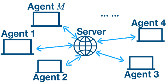
Figure 1: Illustration of Star-shaped Communication Network

We now describe our communication protocol as follows: In this paper we assume the existence of a central server through which all the agents can share their local data (Figure 1). Each agent can communicate with the server by uploading local data and downloading global data from the server. This is also known as the star-shaped communication network (Wang et al., 2020; Dubey & Pentland, 2020; He et al., 2022a).

Moreover, each agent can decide whether to trigger a communication with the server or not. Specifically, at the end of episode $k$, the active agent $m_{k}$ can choose whether to upload its local trajectory to the central server and download all the data uploaded to the server by that time. The communication complexity is measured by the total number of communication rounds between the agents and the server.

Importantly, we consider an asynchronous setting satisfying the following two properties:

• Full participation or a round-robin-type participation is not required.

• The communication between one agent and the server will not cause mandatory download for other agents.

This setting is much more flexible than the synchronous setting where no offline agent is allowed. As a comparison, in Dubey & Pentland (2021), all agents are required to participate in a round-robin fashion. Our setting is more general than the synchronous setting since it gives the agents the extra flexibility to decide whether to participate or not. The pseudo-code of the communication protocol is summarized by Algorithm 1.

Algorithm 1 Communication Protocol

1:  for $k=1,\ldots,K$ do

2:     Agent $m_{k}$ is active

3:     Receives $s_{k,1}$ from the environment

4:     for $h=1,\cdots,H$ do

5:        Take action $a_{k,h}\leftarrow\pi_{k,h}(\cdot|s_{k,h})$

6:        Receive $s_{k,h+1}\sim\mathbb{P}_{h}(\cdot|s_{k,h},a_{k,h})$

7:        Receive reward $r_{k,h}$

8:     end for

9:     if Communication Triggered then

10:        Send local data SERVER.

11:        Download from SERVER

12:        Update policy using all available data

13:     end if

14:  end for

Communication Complexity and Switching Cost.

We define the communication complexity of an algorithm to be the total number of rounds of communication (i.e. one upload and download operation) between any agent and the central server. Note that some papers also use the number of bits to measure the communication complexity (Wang et al., 2020). Here we follow the notation of communication complexity in Dubey & Pentland (2021).

The policy switching cost refers to the number of times the agents change their policies (Kalai & Vempala, 2005; Abbasi-Yadkori et al., 2011). In the RL setting where the agents choose to adopt a greedy policy according to their estimated Q-functions, the switching cost is also equal to the number of times the estimated Q-functions are updated.

Learning Objective.

For any policy $\pi=\{\pi_{h}\}_{h=1}^{H}$, we define the corresponding value functions as

$$V^{\pi}_{h}(s)\coloneqq\mathbb{E}\bigg{[}\sum_{h^{\prime}=h}^{H}r_{h^{\prime}}(s_{h^{\prime}},\pi_{h^{\prime}}(s_{h^{\prime}}))\bigg{|}s_{h}=s\bigg{]},\ \forall h\in[H].$$

Since the horizon $H$ is finite and action space $\mathcal{A}$ is also finite, there exists some optimal policy $\pi^{\star}$ such that

$$V_{h}^{\pi^{\star}}(s)=\sup_{\pi}V_{h}^{\pi}(s),$$

and we denote $V_{h}^{\star}=V_{h}^{\pi^{\star}}$. Due to space limit, more definition details of the value functions and Q-functions can be found in Appendix A.

The objective of all agents is to collaboratively minimize the aggregated cumulative regret defined as

$$R(K) \coloneqq\sum_{k=1}^{K}\left[V^{\star}_{1}(s_{k,1})-V_{1}^{\pi_{m_{k},k}}(s_{k,1})\right],$$ (3.2)

where $m_{k}$ is the active agent in episode $k$, $\pi_{m_{k},k}=\{\pi_{m_{k},k,h}\}_{h=1}^{H}$ is the policy adopted by agent $m_{k}$ in episode $k$, and $s_{k,1}$ is the initial state of episode $k$.

4 The Proposed Algorithm

Now we proceed to present our proposed algorithm, as displayed in Algorithm 2. After explaining the detailed design of Algorithm 2, we will also discuss possible extensions to other MDP settings in Section 4.2. Here for notational convenience, we abbreviate $\bm{\phi}_{k,h}:=\bm{\phi}(s_{k,h},a_{k,h})$.

4.1 Algorithmic Design

Algorithm 2 adopts an execute-then-update framework on a high level: In each episode $k\in[K]$, there is one active agent denoted by $m=m_{k}$ (Line 4 in Algorithm 2). Here we omit the subscript $k$ for better readability. Each episode involves an interaction phase (Line 6-13) and an event-triggered communication and policy update phase (Line 14-26).

Phase I: Interaction.

Agent $m$ will first interact with the environment by executing the greedy policy with respect to its current Q-function estimates $\{Q_{m,k,h}\}_{h=1}^{H}$ (Line 7 & 8), and collect the data from the trajectory of the current episode (Line 9 & 10). Then the agent will update its local dataset and covariance matrices (Line 11 & 12).

Phase II: Communication and Policy Update.

The second phase involving communication and policy update is triggered by a determinant-based criterion (Line 14). Once the criterion is satisfied, the agent will upload all the accumulated local data to the central server (Line 18), and then download all the available data from the server (Line 20). Using this latest dataset, the agent then updates its Q-function estimates (Line 21-23).

More specifically, the Q-function estimate is obtained by using backward least square value iteration following Jin et al. (2020): Given the estimate $Q_{m,k+1,h+1}$ for step $h+1$, we solve for $\mathbf{w}_{m,k+1,h}$ that minimizes the Bellman error in terms of a ridge linear regression:

$$\mathbf{w}_{m,k+1,h} =\bm{\Lambda}_{m,k+1,h}^{-1}\sum_{\tau\in{\mathcal{D}_{m,k,h}}}\bm{\phi}(s_{\tau,h},a_{\tau,h})$$

$$\qquad\cdot\left[r_{\tau,h}+\max_{a}Q_{m,k+1,h+1}(s_{\tau,h+1},a)\right].$$ (4.1)

In the above summation we use $\tau\in\mathcal{D}_{m,k,h}$ to denote the collection of indices of all the episodes whose data is available to agent $m$ by the end of episode $k$. Recall from line 11 of Algorithm 2 that the original definition of $\mathcal{D}_{m,k,h}$ is the dataset of trajectories available to agent $m$. Here we slightly abuse the definition of $\mathcal{D}_{m,k,h}$ to reflect the fact that $\mathbf{w}_{m,k+1,h}$ is computed using only available trajectories to agent $m$ by the end of episode $k$. The Q-function estimate for step $h$ is given by

$$Q_{m,k+1,h}(\cdot,\cdot)$$ (4.2)

$$\quad=\left[\bm{\phi}(\cdot,\cdot)^{\top}\mathbf{w}_{m,k+1,h}+\Gamma_{m,k+1,h}(\cdot,\cdot)\right]_{[0,H-h+1]},$$

where $\Gamma_{m,k+1,h}$ is a bonus term that ensures the optimism of $Q_{m,k+1,h}$, and is defined by

$$\Gamma_{m,k+1,h}(\cdot,\cdot)=\beta\cdot\|\bm{\phi}(\cdot,\cdot)\|_{\bm{\Lambda}_{m,k+1,h}^{-1}}.$$ (4.3)

Otherwise if the criterion is not satisfied, then the local data as well as the Q-function estimates remain unchanged for this agent (Line 27).

Discussion on The Criterion.

The determinant-based criterion is a common and important technique in single-agent contextual bandits (Abbasi-Yadkori et al., 2011; Ruan et al., 2021) and RL with linear function approximation (Zhou et al., 2021c; Wang et al., 2021; Min et al., 2022a), where it is often used to reduce the policy switching cost. While in our multi-agent linear MDP setting, we apply it to determine the appropriate time for communication and the corresponding policy update. The similar idea has been adopted by other works on multi-agent bandits and RL problems (Wang et al., 2020; Li & Wang, 2022; He et al., 2022a; Dubey & Pentland, 2020, 2021).

In our Algorithm 2, the criterion is adjusted by a parameter $\alpha$ that controls the communication frequency: smaller $\alpha$ indicates less frequent communication and larger $\alpha$ implies otherwise. As will be shown in Section 5, $\alpha$ determines the trade-off between the total number of communication rounds (or equivalently, policy updates) and the total regret of Algorithm 2. With a proper choice of $\alpha$, we show that our algorithm achieves a regret nearly identical to that under the single-agent setting (Jin et al., 2020) at a low communication complexity which depends only logarithmically on $K$.

Algorithm 2 Asynchronous Multi-agent LSVI

1:  Input: number of episodes $K$, $\beta$, $\alpha$

2:  Initialize: $\bm{\Lambda}_{m,1,h}\leftarrow\lambda\mathbf{I}_{d\times d}$, $\mathbf{w}_{m,1,h}\leftarrow\mathbf{0}$, $Q_{m,1,h}\leftarrow[\beta[\bm{\phi}(\cdot,\cdot)^{\top}(\bm{\Lambda}_{m,1,h})^{-1}\bm{\phi}(\cdot,\cdot)]^{1/2}]_{[0,H-h+1]}$, $\bm{\Lambda}_{m,0,h}^{\textnormal{loc}}\leftarrow\mathbf{0}$, $\mathcal{D}_{m,0,h}\leftarrow\emptyset$, $\forall\ m,h\in[M]\times[H]$

3:  for $k=1,\ldots,K$ do

4:     Agent $m=m_{k}$ is active

5:     Receive $s_{k,1}$ from the environment

6:     for $h=1,\ldots,H$ do

7:        $\pi_{m,k,h}(\cdot)\leftarrow\mathop{\mathrm{argmax}}_{a\in\mathcal{A}}Q_{m,k,h}(\cdot,a)$

8:        Take action $a_{k,h}\sim\pi_{m,k,h}(\cdot|s_{k,h})$

9:        Receive next state $s_{k,h+1}\sim\mathbb{P}_{h}(\cdot|s_{k,h},a_{k,h})$

10:        Receive reward $r_{k,h}$

11:        $\mathcal{D}_{m,k,h}\leftarrow\mathcal{D}_{m,k-1,h}\cup\{s_{k,h},a_{k,h},s_{k,h+1},r_{k,h}\}$

12:        $\bm{\Lambda}_{m,k,h}^{\textnormal{loc}}\leftarrow\bm{\Lambda}_{m,k-1,h}^{\textnormal{loc}}+\bm{\phi}_{k,h}\bm{\phi}_{k,h}^{\top}$

13:     end for

14:     if $\exists h$ s.t. $\frac{\det(\bm{\Lambda}_{m,k,h}+\bm{\Lambda}_{m,k,h}^{\text{loc}})}{\det(\bm{\Lambda}_{m,k,h})}>1+\alpha$ then

15:        $Q_{m,k+1,H+1}\leftarrow 0$

16:        for $h=H,H-1,\cdots,1$ do

17:           Agent $m$ sends local data to SERVER:

18:           $\bm{\Lambda}_{k,h}^{\textnormal{ser}}\leftarrow\bm{\Lambda}_{k,h}^{\textnormal{ser}}+\bm{\Lambda}_{m,k,h}^{\textnormal{loc}}$, $\mathcal{D}_{k,h}^{\textnormal{ser}}\leftarrow\mathcal{D}_{k,h}^{\textnormal{ser}}\cup\mathcal{D}_{m,k,h}$

19:           SERVER sends global data back to agent $m$:

20:           $\bm{\Lambda}_{m,k+1,h}\leftarrow\bm{\Lambda}_{k,h}^{\text{ser}}$, $\mathcal{D}_{m,k,h}\leftarrow\mathcal{D}_{k,h}^{\textnormal{ser}}$

21:           Update estimate $\mathbf{w}_{m,k+1,h}$ by (4.1)

22:           Update bonus $\Gamma_{m,k+1,h}$ by (4.3)

23:           Update Q-function estimate $Q_{m,k+1,h}$ by (4.2)

24:        end for

25:        Reset $\bm{\Lambda}_{m,k,h}^{\textnormal{loc}}\leftarrow\textbf{0}$, $\forall\ h\in[H]$

26:     else

27:        $Q_{m,k+1,h}\leftarrow Q_{m,k,h}$, $\bm{\Lambda}_{m,k+1,h}\leftarrow\bm{\Lambda}_{m,k,h}$, $\bm{\Lambda}_{k+1,h}^{\textnormal{ser}}\leftarrow\bm{\Lambda}_{k,h}^{\textnormal{ser}}$, $\mathcal{D}_{k+1,h}^{\textnormal{ser}}\leftarrow\mathcal{D}_{k,h}^{\textnormal{ser}}$, $\forall\ h\in[H]$

28:     end if

29:     for all other inactive agents $m^{\prime}\neq m$ do

30:        $Q_{m^{\prime},k+1,h}\leftarrow Q_{m^{\prime},k,h}$, $\bm{\Lambda}_{m^{\prime},k+1,h}\leftarrow\bm{\Lambda}_{m^{\prime},k,h}$, $\forall\ h\in[H]$

31:     end for

32:  end for

4.2 Extension to Other MDP Settings

We remark that though designed for linear MDPs, Algorithm 2 can be easily extended to other MDP settings.

Note that for any tabular MDP with small state and action space, we can represent it using the one-hot feature mapping as discussed in Example 2.1 in Jin et al. (2020). Thus Algorithm 2 can be applied directly to tabular MDPs, and the determinant-based criterion in Line 14 would become a criterion based on the visitation count for every state-action pair. However, we anticipate that Theorem 5.1 would produce in this case an regret upper bound that is suboptimal in $|{\mathcal{S}}|$ and $|\mathcal{A}|$, which is possibly due to that the one-hot feature mapping is not a good representation.

Moreover, the algorithm design can also be applied to linear mixture MDPs where we would have a tenary feature mapping $\phi:{\mathcal{S}}\times\mathcal{A}\times{\mathcal{S}}\to\mathbb{R}^{d}$. Then for example, the UCRL-VTR algorithm (Jia et al., 2020; Ayoub et al., 2020) can be adapted to the asynchronous cooperative setting by designing a similar communication criterion based on the covariance matrix defined over $\phi_{V}(\cdot,\cdot):=\sum_{s\in{\mathcal{S}}}\phi(s,\cdot,\cdot)V(s)$, instead of the $\bm{\Lambda}$ defined over only the feature mapping in our case of linear MDPs.

There have also been other more advanced algorithms for linear MDPs (Hu et al., 2022; He et al., 2022b; Agarwal et al., 2022) that exploit variance information to further reduce the dependence of the regret bound on problem parameters. We leave it as future work to develop and analyze variance-aware variants of Algorithm 2.

5 Main Results

We now present the main theoretical results. We provide the regret upper bound for Algorithm 2 in Theorem 5.1, and compare it with existing related results. Then as a complement, in Theorem 5.5, we provide a lower bound on the communication complexity for cooperative linear MDPs.

5.1 Regret Upper Bound

The following theorem provides the regret upper bound of Algorithm 2.

Theorem 5.1 (Regret Upper Bound).

Under Assumption 3.1, there exists some universal constant $c_{\beta}$ such that by choosing

$$\beta=c_{\beta}dH\widetilde{C}\left[\log\left(\frac{2+K}{\delta\min\{1,\lambda,\alpha\lambda\}}\right)+\log\left(Hd\widetilde{C}\right)\right],$$

where $\widetilde{C}\coloneqq M\sqrt{\alpha}+\sqrt{1+M\alpha}$, then with probability at least $1-\delta$, the regret of Algorithm 2 can be bounded as

$$\mathcal{O}\left(\beta\sqrt{1+M\alpha}H\sqrt{dK\log\left(2dK/\min\{1,\lambda\}\delta\right)}\right).$$

Moreover, the communication complexity and policy switching cost (in number of rounds) are upper bounded by

$$\mathcal{O}\left(dH(M+1/\alpha)\log(1+K/\lambda d)\right).$$

Remark 5.2.

Theorem 5.1 indicates that by setting the parameters $\alpha=1/M^{2}$ and $\lambda=1$ in Algorithm 2, the regret upper bound can be simplified to $\widetilde{\mathcal{O}}(d^{3/2}H^{2}\sqrt{K})$, and the communication complexity is bounded by $\widetilde{\mathcal{O}}(dHM^{2})$.

Remark 5.3.

We compare our upper bound with the best known result by Dubey & Pentland (2021). In their Theorem 1, Dubey & Pentland (2021) present an $\widetilde{\mathcal{O}}(d^{3/2}H^{2}\sqrt{MT})$ regret upper bound for the homogeneous-agent setting (i.e. the same transition kernel and reward functions shared among all agents), which is identical to the multi-agent linear MDP setting considered in our paper. However, their communication protocol is synchronous in a round-robin fashion (see line 4 of their Algorithm 1), and thus $MT$ under their setting is equal to our $K$. Therefore, by Theorem 5.1, our regret upper bound for the asynchronous setting matches that for the synchronous setting.

Remark 5.4.

Our result generalizes that of the multi-agent linear bandit setting (He et al., 2022a) and the single-agent linear MDP setting (Jin et al., 2020). Specifically, with $H=1$, our upper bound becomes $\widetilde{\mathcal{O}}(d\sqrt{K})$ and the number of communication rounds becomes $\widetilde{\mathcal{O}}(dM^{2})$. Note that we save a $\sqrt{d}$ factor in the regret bound compared to the original $d^{3/2}$ dependence from Theorem 5.1 since there is no covering issue when $H=1$. Both the regret and the communication reduce to those under the bandit setting (He et al., 2022a). When $M=1$, our regret reduces to $\tilde{\mathcal{O}}(d^{3/2}H^{2}\sqrt{K})$, matching that of Jin et al. (2020).

5.2 Regret Lower Bound

Theorem 5.5 (Regret Lower Bound).

Suppose $d,H\geq 2$ and number of episodes $K\geq dM$, then for any algorithm Alg with expected communication complexity less than $dM/11400$, there exist a linear MDP, such that the expected regret for algorithm Alg is at least $\Omega(H\sqrt{dMK})$.

Remark 5.6.

Theorem 5.5 suggests that, for any algorithm Alg with communication complexity $o(dM)$, the regret is no better than $\Omega(\sqrt{MK})$. On the other hand, if each agent perform the LSVI-UCB algorithm (Jin et al., 2020), the total regret of $M$ agents is upper bounded by $\sum_{m=1}^{M}\widetilde{O}(\sqrt{K_{m}})=\widetilde{O}(\sqrt{MK})$, where $K_{m}$ is the number of episodes that agent $m$ is active. Thus, in order to improve the performance through collaboration and remove the dependency on the number of agent $M$, an $\Omega(dM)$ communication complexity is necessary.

Remark 5.7.

Though Theorem 5.5 requires the number of stage $H\geq 2$, it is not difficult to extend the result for $H=1$ with stochastic reward function $r_{h}(s,a)$. In this situation, Theorem 5.5 will reduce to bandit problem with adversarial contexts and improves the communication complexity in He et al. (2022a) with a factor of $d$. We also compare our result with the communication lower bound in Amani et al. (2022). In this work, they measured the communication complexity by bits, which is strictly larger than our definition, and also provided a $\Omega(dM)$ communication complexity (in bits) for stochastic contexts.

6 Overview of the Analysis

In this section, we discuss the technical challenges of analyzing Algorithm 2 and our solutions.

6.1 Technical Challenges

The asynchronous communication protocol causes a unique challenge in the theoretical analysis. To illustrate the challenge, let us first recall the synchronous setting with a round-robin-type participation, as studied in Dubey & Pentland (2021). Note that under this setting, the order of participation is fixed. This implies that if $\bm{\phi}_{k,h}$ is uploaded to the server, then for all $k^{\prime}<k$, the vectors $\bm{\phi}_{k^{\prime},h}$ must also have already been uploaded to the server. As a sharp comparison, the above important condition is no longer satisfied under the asynchronous setting. We name the violation of this condition the information asymmetry issue.

Technically, this issue causes two consequences. Recall from the analysis of LSVI-UCB that the final regret bound depends on two technical lemmas: the concentration of self-normalized martingales, and the elliptical potential lemma (Abbasi-Yadkori et al., 2011; Jin et al., 2020). The first lemma determines the width of the confidence region (i.e. $\beta$), and the second is crucial for bounding the sum of the bonus terms (i.e. $\sum_{k=1}^{K}\|\bm{\phi}_{k,h}\|_{\bm{\Lambda}_{m,k,h}^{-1}}$). Both lemmas require a well-defined and fixed order of $\bm{\phi}_{k,h}$ vectors in the collected data in order to be applied. Unfortunately, such an order does not exist in the asynchronous setting, since the data receiving process by the server and every agent is stochastic. The analysis of this stochastic process is also prohibitive because our agents have full freedom to decide whether to participate. Therefore, this arbitrary pattern in the data collected by Algorithm 2 forbids the directly application of these two tools.

To address this information asymmetry issue, we develop a novel form of the self-normalized martingale concentration lemma (Lemma B.4), and an asynchronous elliptical potential lemma (Lemma 6.4). The main idea is a refined analysis of the local covariance matrix $\bm{\Lambda}_{m,k,h}$ and the universal covariance matrix and their comparison under the partial ordering defined by matrix positive definiteness. In the remaining of this section, we overview some key steps and the definition of some important quantities behind the upper bound in Theorem 5.1. The full details are included in Appendix B.

6.2 Key Ingredients of the Proof

For any agent $m\in[M]$ and episode $k\in[K]$, define the following indices:

• $m_{k}$: the active agent of episode $k$. Note that in Algorithm 2 we use $m$ instead of $m_{k}$ due to space limit.

• $t_{k}(m)$: for any agent $m$, $t_{k}(m)\leq k$ is the last episode when agent $m$ adopts a newly updated a policy by the end of episode $k$. If no policy updating has been conducted by the end of episode $k$, then by default $t_{k}(m)=1$.

For the participating agent $m_{k}$ in episode $k$, its adopted Q-function $Q_{m_{k},k,h}$ would be equal to $Q_{m_{k},t_{k},h}$, for all $h\in[H]$, according to the definition. In the following, we may write $t_{k}=t_{k}(m_{k})$ whenever there is no confusion. A comprehensive clarification of notation is also provided in Appendix A.

Regret Decomposition.

By Definition 3.2, the regret is

$$R(K) \coloneqq\sum_{k=1}^{K}\left[V^{\star}_{1}(s_{k,1})-V_{1}^{\pi_{m_{k},k}}(s_{k,1})\right]$$

$$\leq\sum_{k=1}^{K}\left[V_{m_{k},k,1}(s_{k,1})-V_{1}^{\pi_{m_{k},k}}(s_{k,1})\right]$$ (6.1)

$$=\sum_{k=1}^{K}\left[V_{m_{k},t_{k}(m_{k}),1}(s_{k,1})-V_{1}^{\pi_{m_{k},k}}(s_{k,1})\right].$$

The inequality is from the following optimism property, which is standard for UCB-type algorithms.

Lemma 6.1 (Optimism).

Under the setting of Theorem 5.1, on the event of Lemma B.5, for all $k\in[K]$, $h\in[H]$, and $(s,a)\in\mathcal{S}\times\mathcal{A}$, we have $Q^{\star}_{h}(s,a)\leq Q_{m_{k},k,h}(s,a)$.

Proof of Lemma 6.1.

See Appendix C.2. ∎

The last step in (6.2) follows from the definition of $t_{k}(m_{k})$. We then further decompose the terms as

$$V_{m_{k},t_{k},h}(s_{k,h})-V_{h}^{\pi_{m_{k},k}}(s_{k,h})$$

$$=Q_{m_{k},t_{k},h}(s_{k,h},a_{k,h})-Q_{h}^{\pi_{m_{k},k}}(s_{k,h},a_{k,h})$$

$$\leq\bm{\phi}_{k,h}^{\top}\mathbf{w}_{m_{k},t_{k},h}+\beta\sqrt{\bm{\phi}_{k,h}^{\top}\bm{\Lambda}^{-1}_{m_{k},t_{k},h}\bm{\phi}_{k,h}}-\bm{\phi}_{k,h}^{\top}\mathbf{w}^{\pi_{m_{k},k}}_{h}.$$

To analyze the above, we establish the following result.

Lemma 6.2.

Suppose we choose $\beta$ as

$$\beta=c_{\beta}Hd\widetilde{C}\left[\log\left(\frac{2+K}{\delta\min\{1,\lambda,\alpha\lambda\}}\right)+\log\left(Hd\widetilde{C}\right)\right],$$

where $\widetilde{C}\coloneqq M\sqrt{\alpha}+\sqrt{1+M\alpha}$ and $c_{\beta}$ is some universal constant. For any fixed policy $\pi$, on the event of Lemma B.5, for any $k\in[K]$, $h\in[H]$, and $(s,a)\in\mathcal{S}\times\mathcal{A}$, it holds that

$$\left|\bm{\phi}(s,a)^{\top}\left(\mathbf{w}_{m_{k},t_{k},h}-\mathbf{w}^{\pi}_{h}\right)-\mathbb{P}_{h}\left[V_{m_{k},t_{k},h+1}-V^{\pi}_{h+1}\right](s,a)\right|$$

$$\leq\beta\sqrt{\bm{\phi}(s,a)^{\top}\bm{\Lambda}^{-1}_{m_{k},t_{k},h}\bm{\phi}(s,a)}.$$

Proof of Lemma 6.2.

See Appendix C.1. ∎

Taming Information Asymmetry. Lemma 6.2 serves a purpose similar to Lemma B.4 in Jin et al. (2020). However, its proof is more involved due to the discrepancy between $\bm{\Lambda}_{m_{k},t_{k},h}$ and $\lambda\mathbf{I}+\sum_{k^{\prime}=1}^{k-1}\bm{\phi}_{k^{\prime},h}$ under the asynchronous setting. In other words, a random proportion of information is missing from the covariance matrix $\bm{\Lambda}_{m_{k},t_{k},h}$, causing the information asymmetry issue.

To circumvent this issue, we establish a delicate comparison of the covariance matrices (B.3) via several auxiliary matrices (Appendix A.1). By doing so, we can bound the discrepancy between each $\bm{\Lambda}_{m_{k},t_{k},h}$ and the full information matrix $\lambda\mathbf{I}+\sum_{k^{\prime}=1}^{k-1}\bm{\phi}_{k^{\prime},h}$, and then apply the classical concentration argument for self-normalized martingales.

Lemma 6.2 further allows us to apply the standard recursive relation for LSVI-type algorithms (Jin et al., 2020).

Lemma 6.3 (Recursion).

Define $\xi_{k,h}=V_{m_{k},t_{k},h}(s_{k,h})-V_{h}^{\pi_{m_{k},k}}(s_{k,h})$. On the event of Lemma B.5, it holds that

$$\xi_{k,h} \leq\xi_{k,h+1}+\left(\mathbb{E}\left[\xi_{k,h+1}\middle|s_{k,h},a_{k,h}\right]-\xi_{k,h+1}\right)$$

$$\qquad+2\beta\sqrt{\bm{\phi}_{k,h}\bm{\Lambda}_{m_{k},t_{k},h}^{-1}\bm{\phi}_{k,h}}.$$

Proof of Lemma 6.3.

See Appendix C.3. ∎

Asynchronous Elliptical Potential Lemma. Finally, Lemma 6.3 allows us to bound the regret by the sum of bonus terms. However, the standard elliptical potential lemma (Abbasi-Yadkori et al., 2011) still does not apply due to the information asymmetry issue. To this end, we proposed an asynchronous elliptical potential lemma to facilitate the analysis.

Lemma 6.4 (Asynchronous Elliptical Potential).

Let

$$B_{h}=\sum_{h=1}^{H}2\beta\sqrt{\bm{\phi}(s_{k,h},a_{k,h})\bm{\Lambda}_{m_{k},t_{k},h}^{-1}\bm{\phi}(s_{k,h},a_{k,h})}.$$

Under the same assumption of Theorem 5.1, it holds that

$$\sum_{k=1}^{K}\min\left\{V_{m_{k},t_{k}(m_{k}),1}(s_{k,1})-V_{1}^{\pi_{m_{k},k}}(s_{k,1}),B_{h}\right\}$$

$$\leq\mathcal{O}(\beta\sqrt{1+M\alpha}H\sqrt{dK\log\left(2dK/\min\{1,\lambda\}\delta\right)}).$$

Proof of Lemma 6.4.

See Appendix C.8. ∎

With all the above steps, we can finally establish the regret upper bound in Theorem 5.1. The remaining details are provided in Appendix B.

7 Conclusion and Future Work

In this paper we propose a provably efficient algorithm for cooperative multi-agent RL with asynchronous communication, and provide a novel theoretical analysis resolving the challenge of information asymmetry induced by asynchronous communication. We also provide a lower bound on the communication complexity for such a setting.

There are several possible directions for future work. Moreover, the current lower bound in Theorem 5.5 is arguably not tight, and it requires novel construction to exhibit the fundamental trade-off between reducing communication complexity and lowering regret. Also, for the asynchronous communication model, it is important to incorporate other aspects such as agent heterogeneity, environment non-stationarity, privacy and more general function approximation.

Appendix A Clarification of Notation

In this section, we give a comprehensive clarification on the notation used in the algorithm and the analysis.

Throughout the paper, we use $\mathcal{O}(\cdot)$ to hide problem-independent universal constants and $\widetilde{\mathcal{O}}(\cdot)$ to further hide logarithmic factors. We use $(\cdot)_{[a,b]}$ to denote the truncation of values into the range $[a,b]$.

We also present the following table of notations. The $\pi$ in the superscript can be replaced by $\pi_{k}$ or $\pi_{\star}$, where the former refers to the policy in episode $k$, and the latter refers to the optimal policy.

Table 2: Notation

Notation	Meaning
$m_{k}$	the active agent in episode $k$
$\pi_{m,k}=\{\pi_{m,k,h}\}_{h=1}^{H}$	the policy of agent $m$ at episode $k$ (regardless of agent $m$ being active or not)
$\{Q_{m,k,h}\}_{h=1}^{H}$	Q-functions of agent $m$ at episode $k$ in Algorithm 2
$\{V_{m,k,h}\}_{h=1}^{H}$	Value functions of agent $m$ at episode $k$ in Algorithm 2, where $V_{m,k,h}(\cdot)=\mathop{\mathrm{argmax}}_{a}Q_{m,k,h}(\cdot,a)$
$\{V_{h}^{\pi}\}_{h=1}^{H}$	Value functions under policy $\pi$
$\bm{\phi}_{k,h}$	$\bm{\phi}_{k,h}=\bm{\phi}(s_{k,h},a_{k,h})$ for $k\in[K]$ and $h\in[H]$
$\mathbf{w}_{m,k,h},\ \bm{\Lambda}_{m,k,h}$	underlying parameter and covariance matrix of $Q_{m,k,h}$ in Algorithm 2

Indices of available episodes

Recall from line 11 and 20 of Algorithm 2 that the original definition of $\mathcal{D}_{m,k,h}$ is the dataset of trajectories available to agent $m$ by the end of episode $k$. However, in our analysis we may use $\tau\in\mathcal{D}_{m,k,h}$ to denote the collection of indices of all the episodes whose data is available to agent $m$ at the beginning of episode $k$. That is, $\tau\in\mathcal{D}_{m,k,h}$ refers to all the episodes whose trajectories are available to agent $m$ by the end of episode $k$. For example, in (4.1), we use the summation over the indices $\tau\in\mathcal{D}_{m,k,h}$ to reflect that the parameter $\mathbf{w}_{m,k+1,h}$ is computed using only available trajectories (either the agent’s own local trajectories or downloaded ones) by the end of episode $k$. This is a slight abuse of the definition of $\mathcal{D}_{m,k,h}$, since this $\tau\in\mathcal{D}_{m,k,h}$ notation is only required in a summation of this kind in the proof and won’t cause further confusion.

Value and Q-functions

For any policy $\pi=\{\pi_{h}\}_{h=1}^{H}$, we define the corresponding value functions as

$$V^{\pi}_{h}(s)\coloneqq\mathbb{E}\left[\sum_{h^{\prime}=h}^{H}r_{h^{\prime}}(s_{h^{\prime}},\pi_{h^{\prime}}(s_{h^{\prime}}))\middle|s_{h}=s\right],\ \forall\ h\in[H].$$

The Q-functions are defined as

$$Q_{h}^{\pi}(s,a)=r_{h}(s,a)+\mathbb{E}\left[\sum_{h^{\prime}=h+1}^{H}r_{h^{\prime}}(s_{h^{\prime}},\pi_{h^{\prime}}(s_{h^{\prime}}))\middle|s_{h}=s,a_{h}=a\right],\ \forall\ h\in[H].$$

Since the horizon $H$ is finite and action space $\mathcal{A}$ is also finite, there exists some optimal policy $\pi^{\star}$ such that

$$V_{h}^{\pi^{\star}}(s)=\sup_{\pi}V_{h}^{\pi}(s).$$

We denote $V_{h}^{\pi^{\star}}=V_{h}^{\star}$. Furthermore, the above definition implies the following Bellman equations

$$Q_{h}^{\pi}(s,a)=r_{h}(s,a)+\mathbb{P}_{h}V_{h+1}^{\pi}(s,a),\ V_{h}^{\pi}(s)=Q_{h}^{\pi}(s,\pi_{h}(s)),\ \forall\ h\in[H],$$

where $V_{H+1}^{\pi}(\cdot)=0$.

Multi-value quantities.

The following quantities from Algorithm 2 can possibly take two different values in an episode due to the policy update. In our analysis, we assume they refer to the values at the end of the episode $k$, unless otherwise stated.

• $\mathcal{D}_{m,k,h}$; $\mathcal{D}_{k,h}^{\textnormal{ser}}$; $\bm{\Lambda}_{k,h}^{\textnormal{ser}}$; $\bm{\Lambda}_{m,k,h}^{\textnormal{loc}}$.

Indices of episodes.

The following indices of episodes are necessary to the analysis under the asynchronous setting:

• $t_{k}(m)$: $t_{k}(m)\leq k$ is the last episode when agent $m$ adopts a newly updated a policy by the end of episode $k$. If no policy updating has been conducted by the end of episode $k$, then by default $t_{k}(m)=1$.

• $n_{k}(m)$: $n_{k}(m)<t_{k}(m)$ is the most recent episode before $k$ when the agent $m$ updates its policy. This newly updated policy is executed for the first time at episode $t_{k}(m)$. If no policy updating has been conducted before episode $k$ by agent $m$, then by default $n_{k}(m)=0$.

• $N_{k}(m)$: $N_{k}(m)\leq k$ is the last episode that agent $m$ participates up until the end of episode $k$. For example, if agent $m$ participates in episode $k$, then $N_{k}(m)=k$.

The above definition implies $0\leq n_{k}(m)<t_{k}(m)\leq N_{k}(m)\leq k$.

A.1 Auxiliary Matrices

We further define a few notations that will be used extensively in the proof.

Universal information.

We define the following matrix of universal information up to the beginning of episode $k$:

$$\bm{\Lambda}_{k,h}^{\textnormal{all}}=\lambda\mathbf{I}+\sum_{\tau=1}^{k-1}\bm{\phi}_{\tau,h}\bm{\phi}_{\tau,h}^{\top},\ \forall\ h\in[H].$$ (A.1)

Personal information.

We define the uploaded information by agent $m$ until episode $k$ as

$$\bm{\Lambda}_{m,k,h}^{\textnormal{up}}=\sum_{\tau=1,m_{\tau}=m}^{n_{k}(m)}\bm{\phi}_{\tau,h}\bm{\phi}_{\tau,h}^{\top},\ \forall\ h\in[H].$$ (A.2)

Since quantities such as $\bm{\Lambda}_{m,k,h}^{\textnormal{loc}}$ can possibly take two different values during episode $k$ due to the policy update, in the following, we assume all these quantities refer to the value at the end of each episode. The matrix $\bm{\Lambda}_{m,k,h}^{\textnormal{loc}}$ can be rewritten as

$$\bm{\Lambda}_{m,k,h}^{\textnormal{loc}} =\sum_{\tau=n_{k}(m)+1,m_{\tau}=m}^{k}\bm{\phi}_{\tau,h}\bm{\phi}_{\tau,h}^{\top},\ \forall\ h\in[H].$$ (A.3)

Appendix B Proof of Regret Upper Bound

B.1 Basic Properties of the LSVI-type Algorithm

In this section, we list a few basic lemmas for our LSVI-type algorithm. Most of these lemmas are modified from those in Jin et al. (2020). These lemmas are crucial to our regret upper bound.

Lemma B.1 (Lemma B.1 in Jin et al. 2020).

Under Assumption 3.1, for any policy $\pi$, for any $h\in[H]$, let $\mathbf{w}_{h}^{\pi}$ be such that $Q_{h}^{\pi}(\cdot,\cdot)=\langle\bm{\phi}(\cdot,\cdot),\mathbf{w}_{h}^{\pi}\rangle$. Then for all $h\in[H]$, it holds that

$$\|\mathbf{w}_{h}^{\pi}\|\leq 2H\sqrt{d}.$$

Lemma B.2.

Under Assumption 3.1, for any $k\in[K]$ and $h\in[H]$, the estimated parameter $\mathbf{w}_{m,k,h}$ in Algorithm 2 satisfies

$$\left\|\mathbf{w}_{m,k,h}\right\|\leq 2H\sqrt{dk/\lambda}.$$

Proof of Lemma B.2.

See Appendix C.4. ∎

Recall the auxiliary matrices defined in Appendix A.1. The following result describes the partial ordering between them.

Lemma B.3 (Covariance matrix ordering).

Under the setting of Theorem 5.1, it holds that

$$\lambda\mathbf{I}+\sum_{m^{\prime}\in[M]}\bm{\Lambda}_{m^{\prime},k,h}^{\textnormal{up}}\succeq\frac{1}{\alpha}\bm{\Lambda}_{m,k,h}^{\textnormal{loc}},\ \forall\ k,h,m\in[K]\times[H]\times[M].$$ (B.1)

Furthermore, for some $1<\underline{t}\leq\bar{t}\leq K$, suppose agent $m$ is the only participating agent within these episodes (i.e. $m_{k}=m$ for all $k\in[\underline{t},\bar{t}]$), and agent $m$ communicates with the server only at episode $k=\underline{t}$ during $[\underline{t},\bar{t}]$. Then for all $k\in[\underline{t}+1,\bar{t}]$, it holds that

$$\bm{\Lambda}_{m,k,h}\succeq\frac{1}{1+M\alpha}\bm{\Lambda}_{k,h}^{\textnormal{all}},\ \forall\ h\in[H].$$ (B.2)

Proof of Lemma B.3.

See Appendix C.5. ∎

The following two lemmas provides the concentration of self-normalized martingales in the asynchronous setting, where the first lemma applies to a fixed $V$ function, and the second one applies to the $V_{m_{k},t_{k},h+1}$ function in Algorithm 2 via a covering argument. With a proper choice of $\alpha$, the bounds can be reduced to $\widetilde{\mathcal{O}}(H\sqrt{d})$ and $\widetilde{\mathcal{O}}(Hd)$, respectively. These are identical to the result under the single-agent case (Jin et al., 2020).

Lemma B.4.

Under the setting of Theorem 5.1, for any fixed $V\in\mathcal{V}$, with probability at least $1-\delta$, for any $k\in[K]$ and $h\in[H]$, it holds that

$$\left\|\sum_{\tau=1,\tau\in\mathcal{D}_{t_{k},h}^{\textnormal{ser}}}^{t_{k}-1}\bm{\phi}_{\tau,h}\left[V(s_{\tau,h+1})-\mathbb{P}_{h}V(s_{\tau,h},a_{\tau,h})\right]\right\|_{\bm{\Lambda}_{m_{k},t_{k},h}^{-1}}$$

$$\leq 2\left(M\sqrt{\alpha}+\sqrt{1+M\alpha}\right)\cdot H\cdot\left(\sqrt{\log\left(\left(\frac{K+\alpha\lambda}{\alpha\lambda}\right)^{d/2}\right)+\log\left(\left(\frac{K+\lambda}{\lambda}\right)^{d/2}\right)+2\log\left(\frac{1}{\delta}\right)}\right).$$

Proof of Lemma B.4.

See Appendix C.6. ∎

Lemma B.5.

Under the setting of Theorem 5.1, with probability at least $1-\delta$, for any $k\in[K]$ and $h\in[H]$, it holds that

$$\left\|\sum_{\tau=1,\tau\in\mathcal{D}_{t_{k},h}^{\textnormal{ser}}}^{t_{k}-1}\bm{\phi}_{\tau,h}\left[V_{m_{k},t_{k},h+1}(s_{\tau,h+1})-\mathbb{P}_{h}V_{m_{k},t_{k},h+1}(s_{\tau,h},a_{\tau,h})\right]\right\|_{\bm{\Lambda}_{m_{k},t_{k},h}^{-1}}$$

$$\leq C(M\sqrt{\alpha}+\sqrt{1+M\alpha})H\sqrt{\iota}+CdH/\sqrt{\lambda},$$

where $C$ is some universal constant and

$$\iota\coloneqq d\log\left(\frac{K+\alpha\lambda}{\alpha\lambda}\right)+d\log\left(\frac{K+\lambda}{\lambda}\right)+\log\frac{1}{\delta}+d\log\left(2+\frac{8k^{3}}{\lambda}\right)+d^{2}\log\left(1+\frac{8\beta^{2}k^{2}}{\lambda d^{1.5}H^{2}}\right).$$

Proof of Lemma B.5.

See Appendix C.7. ∎

The next lemma is applied to bound the number of communication rounds of Algorithm 2. We first divide the episodes into different epochs.

Lemma B.6.

For each $i\geq 0$, define $\widetilde{K}_{i}=\min\left\{k\in[K]:\ \exists h\in[H]\ \textnormal{s.t.}\ \det(\bm{\Lambda}_{k,h}^{\textnormal{all}})\geq 2^{i}\lambda^{d}\right\}$. Divide all episodes into epochs where epoch i is given as $\{\widetilde{K}_{i},\widetilde{K}_{i}+1,\cdots,\widetilde{K}_{i+1}-1\}$, where $i\geq 0$. Then within any epoch $i$, the total number of communication rounds is upper bounded by $\mathcal{O}(H(M+1/\alpha))$.

Proof of Lemma B.6.

The proof follows from the a modified argument from that of Lemma 6.2 in (He et al., 2022a). Different from He et al. (2022a), by Line 14 of Algorithm 2, a communication is triggered if any of the $H$ determinant conditions are satisfied. As a result, the communication number is at most $H$ times the upper bound in Lemma 6.2 in He et al. (2022a). ∎

B.2 Proof of Theorem 5.1

Proof of Theorem 5.1.

We first prove the regret upper bound. By Lemma 6.1, the regret can be upper bounded as

$$R(K) =\sum_{k=1}^{K}\left[V^{\star}_{1}(s_{k,1})-V_{1}^{\pi_{m_{k},k}}(s_{k,1})\right]$$

$$\leq\sum_{k=1}^{K}\left[V_{m_{k},k,1}(s_{k,1})-V_{1}^{\pi_{m_{k},k}}(s_{k,1})\right]$$

$$=\sum_{k=1}^{K}\left[V_{m_{k},t_{k}(m_{k}),1}(s_{k,1})-V_{1}^{\pi_{m_{k},k}}(s_{k,1})\right]$$

$$\leq\sum_{k=1}^{K}\sum_{h=1}^{H}\left(\mathbb{E}\left[\xi_{k,h+1}\middle|s_{k,h},a_{k,h}\right]-\xi_{k,h+1}\right)$$

$$+\sum_{k=1}^{K}\min\left\{V_{m_{k},t_{k}(m_{k}),1}(s_{k,1})-V_{1}^{\pi_{m_{k},k}}(s_{k,1}),\ \sum_{h=1}^{H}2\beta\sqrt{\bm{\phi}(s_{k,h},a_{k,h})\bm{\Lambda}_{m_{k},t_{k},h}^{-1}\bm{\phi}(s_{k,h},a_{k,h})}\right\},$$ (B.3)

where the first inequality is by Lemma 6.1, and the second inequality is by Lemma 6.3. The minimum in the last step might seems odd at first, but will turn out to be necessary later. Bounding the first term in the above is straightforward using martingale convergence (Jin et al., 2020). Specifically, by the definition of in Lemma 6.3, the first term can be written as

$$\sum_{k=1}^{K}\sum_{h=1}^{H}\left(\mathbb{E}\left[\xi_{k,h+1}\middle|s_{k,h},a_{k,h}\right]-\xi_{k,h+1}\right)$$

$$=\sum_{k=1}^{K}\sum_{h=1}^{H}\left(\mathbb{E}\left[[V_{m_{k},t_{k},h+1}(s_{k,h+1})-V_{h+1}^{\pi_{m_{k},k}}(s_{k,h+1})]\middle|s_{k,h+1},a_{k,h+1}\right]-[V_{m_{k},t_{k},h+1}(s_{k,h+1})-V_{h+1}^{\pi_{m_{k},k}}(s_{k,h+1})]\right)$$

Above summation can be viewed as the sum of a martingale difference sequence since $V_{m_{k},t_{k},h+1}$ and $V_{h+1}^{\pi_{m_{k},k}}$ are independent of the observation in episode $k$. Since $|V_{m_{k},t_{k},h+1}(s_{k,h+1})-V_{h+1}^{\pi_{m_{k},k}}(s_{k,h+1})|\leq 2H$, by Azuma-Hoeffding inequality, with probability at least $1-\delta$, for all $k,h$, it holds that

$$\sum_{k=1}^{K}\sum_{h=1}^{H}\left(\mathbb{E}\left[\xi_{k,h+1}\middle|s_{k,h},a_{k,h}\right]-\xi_{k,h+1}\right)\leq 2H^{3/2}\sqrt{K\log(2/\delta)},$$ (B.4)

where $\{\xi_{k,h}\}_{k,h\in[K]\times[H]}$ are defined in Lemma 6.3. For the second term, note that instead of bounding $2\beta\sum_{k=1}^{K}\sum_{h=1}^{H}\sqrt{\bm{\phi}(s_{k,h},a_{k,h})\bm{\Lambda}_{m_{k},t_{k},h}^{-1}\bm{\phi}(s_{k,h},a_{k,h})}$ directly, we construct a new term involving a minimum between the bonus and the per-episode regret bound $V_{m_{k},t_{k}(m_{k}),1}(s_{k,1})-V_{1}^{\pi_{m_{k},k}}(s_{k,1})$. The reason behind this is that the sum of bonus along cannot be bounded using the standard elliptical potential argument (Abbasi-Yadkori et al., 2011) due to the asynchronous nature of the communication protocol. Its analysis turns out to be much more involved and therefore is summarized separately in Lemma 6.4. Now, combining Lemma 6.4 and (B.4), we finish the proof of the regret upper bound.

The proof of the communication complexity of Algorithm 2 is straightforward given the simple form of our determinant-based criterion. By Lemma B.6, it remains to bound the number of epochs. Recall from Assumption 3.1 that $\|\bm{\phi}(\cdot,\cdot)\|\leq 1$. This implies that, for any $h\in[H]$,

$$\det(\bm{\Lambda}_{K,h}^{\textnormal{all}})\leq\left(\lambda+\frac{1}{d}\sum_{k=1}^{K}\|\bm{\phi}_{k,h}\|_{2}^{2}\right)^{d}\leq\lambda^{d}\left(1+\frac{K}{\lambda d}\right)^{d}.$$

By the definition of $\widetilde{K}_{i}$ from Lemma B.6, in order for $\widetilde{K}_{i}$ to be non-empty, $i$ should satisfy

$$2^{i}\lambda^{d}\leq\lambda^{d}\left(1+\frac{K}{\lambda d}\right)^{d},$$

which implies $i\leq\log 2\cdot d\log(1+K/\lambda d)$. Together with Lemma B.6, the total communication number is upper bounded by $H(M+1/\alpha)\cdot\log 2\cdot d\log(1+K/\lambda d)$ up to some constant factor. This finishes the proof. ∎

Appendix C Proof of Technical Lemmas

C.1 Proof of Lemma 6.2

Proof of Lemma 6.2.

Recall the definition of $\mathbf{w}_{m,k+1,h}$ from (4.1), and the definition of $n_{k}(\cdot)$ from Appendix A. Then since $\mathbf{w}_{m_{k},k,h}=\mathbf{w}_{m_{k},t_{k},h}$ is computed using all the trajectories available to agent $m_{k}$ by the beginning episode $t_{k}$, we can write

$$\mathbf{w}_{m_{k},t_{k},h}=\bm{\Lambda}_{m_{k},t_{k},h}^{-1}\sum_{\tau=1,\tau\in\mathcal{D}_{n_{k}(m_{k}),h}^{\textnormal{ser}}}^{t_{k}-1}\bm{\phi}_{\tau,h}\cdot\left[r_{\tau,h}+V_{m_{k},t_{k},h+1}(s_{\tau,h+1})\right],$$

where $\tau\in\mathcal{D}_{n_{k}(m_{k}),h}^{\textnormal{ser}}$ denotes all the data uploaded to the server by the end of episode $n_{k}$. Note that this is well-defined since $n_{k}(m_{k})$ is the most recent episode before $k$ when agent $m_{k}$ updates its policy, and therefore its local data is also included in $\mathcal{D}_{n_{k}(m_{k}),h}^{\textnormal{ser}}$. In the following we simply use $n_{k}$ instead of $n_{k}(m_{k})$ since there is no confusion. We then write

$$\mathbf{w}_{m_{k},t_{k},h}-\mathbf{w}^{\pi}_{h}$$

$$=\bm{\Lambda}_{m_{k},t_{k},h}^{-1}\sum_{\tau=1,\tau\in\mathcal{D}_{n_{k},h}^{\textnormal{ser}}}^{t_{k}-1}\bm{\phi}_{\tau,h}\cdot\left[r_{\tau,h}+V_{m_{k},t_{k},h+1}(s_{\tau,h+1})\right]-\mathbf{w}^{\pi}_{h}$$

$$=\bm{\Lambda}_{m_{k},t_{k},h}^{-1}\left\{-\lambda\mathbf{w}^{\pi}_{h}+\sum_{\tau=1,\tau\in\mathcal{D}_{n_{k},h}^{\textnormal{ser}}}^{t_{k}-1}\bm{\phi}_{\tau,h}\left[V_{m_{k},t_{k},h+1}(s_{\tau,h+1})-\mathbb{P}_{h}V_{h+1}^{\pi}(s_{\tau,h},a_{\tau,h})\right]\right\}$$

$$=-\underbrace{\lambda\bm{\Lambda}_{m_{k},t_{k},h}^{-1}\mathbf{w}^{\pi}_{h}}_{\mathbf{v}_{1}}+\underbrace{\bm{\Lambda}_{m_{k},t_{k},h}^{-1}\sum_{\tau=1,\tau\in\mathcal{D}_{n_{k},h}^{\textnormal{ser}}}^{t_{k}-1}\bm{\phi}_{\tau,h}\left[V_{m_{k},t_{k},h+1}(s_{\tau,h+1})-\mathbb{P}_{h}V_{m_{k},t_{k},h+1}(s_{\tau,h},a_{\tau,h})\right]}_{\mathbf{v}_{2}}$$

$$\qquad+\underbrace{\bm{\Lambda}_{m_{k},t_{k},h}^{-1}\sum_{\tau=1,\tau\in\mathcal{D}_{n_{k},h}^{\textnormal{ser}}}^{t_{k}-1}\bm{\phi}_{\tau,h}\mathbb{P}_{h}\left[V_{m_{k},t_{k},h+1}-V_{h+1}^{\pi}\right](s_{\tau,h},a_{\tau,h})}_{\mathbf{v}_{3}}.$$ (C.1)

For the first term, we have

$$\left|\bm{\phi}(s,a)^{\top}\mathbf{v}_{1}\right|\leq\sqrt{\lambda}\left\|\mathbf{w}_{h}^{\pi}\right\|_{2}\sqrt{\bm{\phi}(s,a)^{\top}\bm{\Lambda}^{-1}_{m_{k},t_{k},h}\bm{\phi}(s,a)}\leq 2H\sqrt{d\lambda}\sqrt{\bm{\phi}(s,a)^{\top}\bm{\Lambda}^{-1}_{m_{k},t_{k},h}\bm{\phi}(s,a)},$$ (C.2)

where the first step is by $\bm{\Lambda}^{-1}_{m_{k},t_{k},h}\preccurlyeq\lambda^{-1}\mathbf{I}$ and the second step is by Lemma B.1. For the second term, we have

$$\left|\bm{\phi}(s,a)^{\top}\mathbf{v}_{2}\right|$$

$$\leq\underbrace{\left\|\sum_{\tau=1,\tau\in\mathcal{D}_{n_{k},h}^{\textnormal{ser}}}^{t_{k}-1}\bm{\phi}_{\tau,h}\left[V_{m_{k},t_{k},h+1}(s_{\tau,h+1})-\mathbb{P}_{h}V_{m_{k},t_{k},h+1}(s_{\tau,h},a_{\tau,h})\right]\right\|_{\bm{\Lambda}_{m_{k},t_{k},h}^{-1}}}_{\chi}\cdot\sqrt{\bm{\phi}(s,a)^{\top}\bm{\Lambda}^{-1}_{m_{k},t_{k},h}\bm{\phi}(s,a)}.$$ (C.3)

For the third term, we have

$$\bm{\phi}(s,a)^{\top}\mathbf{v}_{3}$$ (C.4)

$$=\left\langle\bm{\phi}(s,a),\bm{\Lambda}_{m_{k},t_{k},h}^{-1}\sum_{\tau=1,\tau\in\mathcal{D}_{n_{k},h}^{\textnormal{ser}}}^{t_{k}-1}\bm{\phi}_{\tau,h}\mathbb{P}_{h}\left[V_{m_{k},t_{k},h+1}-V_{h+1}^{\pi}\right](s_{\tau,h},a_{\tau,h})\right\rangle$$

$$\leq\left\langle\bm{\phi}(s,a),\bm{\Lambda}_{m_{k},t_{k},h}^{-1}\sum_{\tau=1,\tau\in\mathcal{D}_{n_{k},h}^{\textnormal{ser}}}^{t_{k}-1}\bm{\phi}_{\tau,h}\bm{\phi}_{\tau,h}^{\top}\int\left[V_{m_{k},t_{k},h+1}-V_{h+1}^{\pi}\right](s^{\prime})\mathrm{d}\bm{\mu}_{h}(s^{\prime})\right\rangle$$

$$\leq\left\langle\bm{\phi}(s,a),\int\left[V_{m_{k},t_{k},h+1}-V_{h+1}^{\pi}\right](s^{\prime})\mathrm{d}\bm{\mu}_{h}(s^{\prime})\right\rangle$$

$$\qquad-\lambda\left\langle\bm{\phi}(s,a),\bm{\Lambda}_{m_{k},t_{k},h}^{-1}\int\left[V_{m_{k},t_{k},h+1}-V_{h+1}^{\pi}\right](s^{\prime})\mathrm{d}\bm{\mu}_{h}(s^{\prime})\right\rangle$$

$$=\mathbb{P}_{h}\left[V_{m_{k},t_{k},h+1}-V_{h+1}^{\pi}\right](s,a)-\lambda\left\langle\bm{\phi}(s,a),\bm{\Lambda}_{m_{k},t_{k},h}^{-1}\int\left[V_{m_{k},t_{k},h+1}-V_{h+1}^{\pi}\right](s^{\prime})\mathrm{d}\bm{\mu}_{h}(s^{\prime})\right\rangle$$

$$\leq\mathbb{P}_{h}\left[V_{m_{k},t_{k},h+1}-V_{h+1}^{\pi}\right](s,a)+2H\sqrt{d\lambda}\cdot\sqrt{\bm{\phi}(s,a)\bm{\Lambda}_{m_{k},t_{k},h}^{-1}\bm{\phi}(s,a)},$$ (C.5)

where the last step holds because $\|\bm{\mu}_{h}\|\leq\sqrt{d}$ by Assumption 3.1. Combining (C.1), (C.2), (C.1) and (C.4), we have

$$\left|\bm{\phi}(s,a)^{\top}(\mathbf{w}_{m_{k},t_{k},h}-\mathbf{w}^{\pi}_{h})-\mathbb{P}_{h}\left[V_{m_{k},t_{k},h+1}-V_{h+1}^{\pi}\right](s,a)\right|$$

$$\leq\left(4H\sqrt{d\lambda}+\chi\right)\cdot\sqrt{\bm{\phi}(s,a)\bm{\Lambda}_{m_{k},t_{k},h}^{-1}\bm{\phi}(s,a)}.$$ (C.6)

It remains to show that the choice of $\beta$ satisfies

$$4H\sqrt{d\lambda}+\chi\leq\beta.$$

By Lemma B.5, we want to show

$$4H\sqrt{d\lambda}+C(M\sqrt{\alpha}+\sqrt{1+M\alpha})H\sqrt{\iota}+CdH/\sqrt{\lambda}\leq\beta.$$

Plugging in the choice of $\beta$ and the definition of $\iota$ from Lemma B.5 and simplifying the expression, it suffices to show that there exists $c_{\beta}$ such that

$$C\left[\log\left(2+\frac{K}{\delta\min\{1,\lambda,\alpha\lambda\}}\right)+\log\left(c_{\beta}Hd(M\sqrt{\alpha}+\sqrt{1+M\alpha})\right)\right]$$

$$\leq c_{\beta}^{2}\left[\log\left(2+\frac{K}{\delta\min\{1,\lambda,\alpha\lambda\}}\right)+\log\left(Hd(M\sqrt{\alpha}+\sqrt{1+M\alpha})\right)\right],$$

where $C$ is some universal constant. The existence of such $c_{\beta}$ is clear. Therefore, we conclude that

$$\left|\bm{\phi}(s,a)^{\top}\left(\mathbf{w}_{m_{k},t_{k},h}-\mathbf{w}^{\pi}_{h}\right)-\mathbb{P}_{h}\left[V_{m_{k},t_{k},h+1}-V^{\pi}_{h+1}\right](s,a)\right|\leq\beta\sqrt{\bm{\phi}(s,a)^{\top}\bm{\Lambda}^{-1}_{m_{k},t_{k},h}\bm{\phi}(s,a)}.$$

∎

C.2 Proof of Lemma 6.1

Proof of Lemma 6.1.

The proof follows from the same induction argument in Lemma B.5 of (Jin et al., 2020). For completeness we introduce the proof here. For step $H$, by Lemma 6.2, we have

$$\left|\bm{\phi}(s,a)^{\top}\mathbf{w}_{m_{k},t_{k},H}-Q^{\star}_{H}(s,a)\right|\leq\beta\sqrt{\bm{\phi}(s,a)^{\top}\bm{\Lambda}^{-1}_{m_{k},t_{k},H}\bm{\phi}(s,a)},$$

since $V_{m_{k},t_{k},H+1}=V^{\star}_{H+1}=0$. This implies

$$Q^{\star}_{H}(s,a)\leq\bm{\phi}(s,a)^{\top}\mathbf{w}_{m_{k},t_{k},H}+\beta\sqrt{\bm{\phi}(s,a)^{\top}\bm{\Lambda}^{-1}_{m_{k},t_{k},H}\bm{\phi}(s,a)}\leq Q_{m_{k},t_{k},H}(s,a).$$

Now suppose we have proved $Q^{\star}_{h+1}(s,a)\leq Q_{m_{k},t_{k},h+1}(s,a)$. Then by Lemma 6.2 again, we have

$$Q^{\star}_{h}(s,a)+\mathbb{P}_{h}\left[V_{m_{k},t_{k},h+1}-V^{\star}_{h+1}\right](s,a)-\bm{\phi}(s,a)^{\top}\mathbf{w}_{m_{k},t_{k},h}\leq\beta\sqrt{\bm{\phi}(s,a)^{\top}\bm{\Lambda}^{-1}_{m_{k},t_{k},h}\bm{\phi}(s,a)},$$

which implies

$$Q^{\star}_{h}(s,a) \leq\bm{\phi}(s,a)^{\top}\mathbf{w}_{m_{k},t_{k},h}+\beta\sqrt{\bm{\phi}(s,a)^{\top}\bm{\Lambda}^{-1}_{m_{k},t_{k},h}\bm{\phi}(s,a)}-\mathbb{P}_{h}\left[V_{m_{k},t_{k},h+1}-V^{\star}_{h+1}\right](s,a)$$

$$\leq\bm{\phi}(s,a)^{\top}\mathbf{w}_{m_{k},t_{k},h}+\beta\sqrt{\bm{\phi}(s,a)^{\top}\bm{\Lambda}^{-1}_{m_{k},t_{k},h}\bm{\phi}(s,a)},$$

where the last step is by the induction hypothesis that $V_{m_{k},t_{k},h+1}-V^{\star}_{h+1}\geq 0$. Therefore, we conclude that

$$Q^{\star}_{h}(s,a) =\min\{H-h+1,Q^{\star}_{h}(s,a)\}$$

$$\leq\min\{H-h+1,\bm{\phi}(s,a)^{\top}\mathbf{w}_{m_{k},t_{k},h}+\beta\sqrt{\bm{\phi}(s,a)^{\top}\bm{\Lambda}^{-1}_{m_{k},t_{k},h}\bm{\phi}(s,a)}\}=Q_{m_{k},t_{k},h}=Q_{m_{k},k,h}.$$

∎

C.3 Proof of Lemma 6.3

Proof of Lemma 6.3.

Lemma 6.2 and the definition of $Q_{m_{k},t_{k},h}$ imply that for any $k,h$ ,

$$Q_{m_{k},t_{k},h}(s_{k,h},a_{k,h})-Q_{h}^{\pi_{m_{k},k}}(s_{k,h},a_{k,h}) \leq\mathbb{P}_{h}\left[V_{m_{k},t_{k},h+1}-V^{\pi_{m_{k},k}}_{h+1}\right](s_{k,h},a_{k,h})+2\beta\sqrt{\bm{\phi}_{k,h}^{\top}\bm{\Lambda}^{-1}_{m_{k},t_{k},h}\bm{\phi}_{k,h}}.$$

By the definition of $V_{m_{k},t_{k},h+1}$ and $V^{\pi_{m_{k},k}}_{h+1}$, we have $\xi_{k,h}=Q_{m_{k},t_{k},h}(s_{k,h},a_{k,h})-Q_{h}^{\pi_{m_{k},k}}(s_{k,h},a_{k,h})$, and it follows that

$$\xi_{k,h}\leq\mathbb{E}[\xi_{k,h+1}|s_{k,h},a_{k,h}]+2\beta\sqrt{\bm{\phi}(s_{k,h},a_{k,h})\bm{\Lambda}_{m_{k},t_{k},h}^{-1}\bm{\phi}(s_{k,h},a_{k,h})}.$$

∎

C.4 Proof of Lemma B.2

Proof of Lemma B.2.

The proof follows from that of Lemma B.2 in (Jin et al., 2020). Specifically, the estimated parameters $\mathbf{w}_{m,k,h}$ take the same form as $\mathbf{w}_{h}^{k}$’s in (Jin et al., 2020) if we re-index the vectors $\bm{\phi}_{k,h}$’s that are available to agent $m$ at episode $k$. ∎

C.5 Proof of Lemma B.3

Proof of Lemma B.3.

Fix some episode $k$ and agent $m$. Recall from Appendix A that $N_{k}(m)\leq k$ is the last episode that agent $m$ participates up until the end of episode $k$. If agent $m$ communicates with server in episode $N_{k}(m)$, then

$$\lambda\mathbf{I}+\sum_{m^{\prime}\in[M]}\bm{\Lambda}_{m^{\prime},k,h}^{\textnormal{up}}\succeq\mathbf{0}=\bm{\Lambda}_{m,N_{k}(m),h}^{\textnormal{loc}}=\bm{\Lambda}_{m,k,h}^{\textnormal{loc}}.$$

If agent $m$ does not participates in episode $N_{k}(m)$, then by Line 14 of Algorithm 2, it holds that, for all $h\in[H]$,

$$\det(\bm{\Lambda}_{m,N_{k}(m),h}+\bm{\Lambda}_{m,N_{k}(m),h}^{\text{loc}})\leq(1+\alpha)\det(\bm{\Lambda}_{m,N_{k}(m),h}).$$

Since no further participation happens between $[N_{k}(m)+1,k]$, above implies

$$\det(\bm{\Lambda}_{m,k,h}+\bm{\Lambda}_{m,k,h}^{\text{loc}})\leq(1+\alpha)\det(\bm{\Lambda}_{m,k,h}).$$

Applying Lemma E.2, we get

$$\frac{\mathbf{x}^{\top}(\bm{\Lambda}_{m,k,h}+\bm{\Lambda}_{m,k,h}^{\text{loc}})\mathbf{x}}{\mathbf{x}^{\top}\bm{\Lambda}_{m,k,h}\mathbf{x}}\leq\frac{\det(\bm{\Lambda}_{m,k,h}+\bm{\Lambda}_{m,k,h}^{\text{loc}})}{\det(\bm{\Lambda}_{m,k,h})}\leq 1+\alpha,$$

and it follows that

$$\mathbf{x}^{\top}\bm{\Lambda}_{m,k,h}^{\text{loc}}\mathbf{x}\leq\alpha\mathbf{x}^{\top}\bm{\Lambda}_{m,k,h}\mathbf{x}.$$

Finally, we conclude that

$$\lambda\mathbf{I}+\sum_{m^{\prime}\in[M]}\bm{\Lambda}_{m^{\prime},k,h}^{\textnormal{up}}\succeq\bm{\Lambda}_{m,k,h}\succeq\frac{1}{\alpha}\bm{\Lambda}_{m,k,h}^{\textnormal{loc}},$$

where the first step follows from the fact that $\bm{\Lambda}_{m,k,h}$ is downloaded at some episode $n_{k}(m)<k$, and the definition of $\bm{\Lambda}_{m^{\prime},k,h}^{\textnormal{up}}$ from (A.2). This proves (B.1).

To show (B.2), suppose that agent $m$ communicates with the server at episode $\underline{t}$, and is active for $k\in[\underline{t},\bar{t}]$. Applying (B.1) for all $M$ agents and averaging, we have

$$\lambda\mathbf{I}+\sum_{m^{\prime}\in[M]}\bm{\Lambda}_{m^{\prime},k,h}^{\textnormal{up}}\succeq\frac{1}{\alpha M}\sum_{m^{\prime}\in[M]}\bm{\Lambda}_{m^{\prime},k,h}^{\textnormal{loc}},$$

and it follows that, for $k\in[\underline{t}+1,\bar{t}]$,

$$\bm{\Lambda}_{m,k,h} =\lambda\mathbf{I}+\sum_{m^{\prime}\in[M]}\bm{\Lambda}_{m^{\prime},\underline{t}+1,h}^{\textnormal{up}}$$

$$=\lambda\mathbf{I}+\sum_{m^{\prime}\in[M]}\bm{\Lambda}_{m^{\prime},k,h}^{\textnormal{up}}$$

$$\succeq\frac{1}{1+\alpha M}\left(\lambda\mathbf{I}+\sum_{m^{\prime}\in[M]}\bm{\Lambda}_{m^{\prime},k,h}^{\textnormal{up}}+\sum_{m^{\prime}\in[M]}\bm{\Lambda}_{m^{\prime},k,h}^{\textnormal{loc}}\right)$$

$$=\frac{1}{1+\alpha M}\bm{\Lambda}_{k,h}^{\textnormal{all}}.$$

Here the first step follows from the definition of $\bm{\Lambda}_{m^{\prime},\underline{t}+1,h}^{\textnormal{up}}$ from (A.2) and the assumption that agent $m$ communicates with the server in episode $\underline{t}$. The second step holds because agent $m$ is the only active agent between $[\underline{t},\bar{t}]$ and thus no further upload has been made by any agent during episodes $[\underline{t}+1,\bar{t}]$. The last step follows from the definition of $\bm{\Lambda}_{k,h}^{\textnormal{all}}$ and the assumption that agent $m$ is the only active agent between $[\underline{t},\bar{t}]$ (i.e. no other agent can upload during $[\underline{t},\bar{t}]$). This finishes the proof of (B.2) and that of Lemma B.3. ∎

C.6 Proof of Lemma B.4

Proof of Lemma B.4.

Define $\eta_{\tau,h}=V(s_{\tau,h+1})-\mathbb{P}_{h}V(s_{\tau,h},a_{\tau,h})$, and

$$\mathbf{u}_{k,h}^{\textnormal{up}}(m^{\prime}) =\sum_{\tau=1,\tau\in\mathcal{D}_{k,h}^{\textnormal{ser}},m_{\tau}=m^{\prime}}^{k}\bm{\phi}_{\tau,h}\eta_{\tau,h},$$

$$\mathbf{u}_{k,h}^{\textnormal{loc}}(m^{\prime}) =\sum_{\tau=1,\tau\notin\mathcal{D}_{k,h}^{\textnormal{ser}},m_{\tau}=m^{\prime}}^{k}\bm{\phi}_{\tau,h}\eta_{\tau,h},$$ (C.7)

for all $m^{\prime}\in[M]$ and $k,h\in[K]\times[H]$. Then we have

$$\left\|\sum_{\tau=1,\tau\in\mathcal{D}_{n_{k},h}^{\textnormal{ser}}}^{t_{k}-1}\bm{\phi}_{\tau,h}\left[V(s_{\tau,h+1})-\mathbb{P}_{h}V(s_{\tau,h},a_{\tau,h})\right]\right\|_{\bm{\Lambda}_{m_{k},t_{k},h}^{-1}}$$

$$=\left\|\sum_{\tau=1,\tau\in\mathcal{D}_{n_{k},h}^{\textnormal{ser}}}^{t_{k}-1}\bm{\phi}_{\tau,h}\eta_{\tau,h}\right\|_{\bm{\Lambda}_{m_{k},t_{k},h}^{-1}}$$

$$=\left\|\sum_{m^{\prime}=1}^{M}\mathbf{u}_{n_{k},h}^{\textnormal{up}}(m^{\prime})\right\|_{\bm{\Lambda}_{m_{k},t_{k},h}^{-1}}$$

$$=\left\|\sum_{m^{\prime}=1}^{M}\mathbf{u}_{n_{k},h}^{\textnormal{up}}(m^{\prime})+\sum_{m^{\prime}=1}^{M}\mathbf{u}_{n_{k},h}^{\textnormal{loc}}(m^{\prime})-\sum_{m^{\prime}=1}^{M}\mathbf{u}_{n_{k},h}^{\textnormal{loc}}(m^{\prime})\right\|_{\bm{\Lambda}_{m_{k},t_{k},h}^{-1}}$$

$$\leq\underbrace{\left\|\sum_{m^{\prime}=1}^{M}\mathbf{u}_{n_{k},h}^{\textnormal{up}}(m^{\prime})+\sum_{m^{\prime}=1}^{M}\mathbf{u}_{n_{k},h}^{\textnormal{loc}}(m^{\prime})\right\|_{\bm{\Lambda}_{m_{k},t_{k},h}^{-1}}}_{(\textnormal{I})}+\underbrace{\left\|\sum_{m^{\prime}=1}^{M}\mathbf{u}_{n_{k},h}^{\textnormal{loc}}(m^{\prime})\right\|_{\bm{\Lambda}_{m_{k},t_{k},h}^{-1}}}_{(\textnormal{II})},$$ (C.8)

where the first and the second steps are by the definition of $\eta_{\tau,h}$ and $\mathbf{u}_{n_{k},h}^{\textnormal{up}}$, and the last step is by triangle inequality.

For $(\textnormal{I})$, we have that with probability at least $1-\delta$, for all $k$,

$$(\textnormal{I}) =\left\|\sum_{\tau=1}^{n_{k}}\bm{\phi}_{\tau,h}\eta_{\tau,h}\right\|_{\bm{\Lambda}_{m_{k},t_{k},h}^{-1}}$$

$$=\left\|\sum_{\tau=1}^{n_{k}}\bm{\phi}_{\tau,h}\eta_{\tau,h}\right\|_{\bm{\Lambda}_{m_{k},n_{k}+1,h}^{-1}}$$

$$\leq\sqrt{1+\alpha M}\left\|\sum_{\tau=1}^{n_{k}}\bm{\phi}_{\tau,h}\eta_{\tau,h}\right\|_{(\bm{\Lambda}_{n_{k}+1,h}^{\textnormal{all}})^{-1}}$$

$$\leq\sqrt{1+\alpha M}\cdot\sqrt{4H^{2}\left[\log\left(\left(\frac{K+\lambda}{\lambda}\right)^{d/2}\right)+\log\left(\frac{1}{\delta}\right)\right]}.$$ (C.9)

Here the first inequality is given by (B.2) in Lemma B.3. The second inequality is derived by applying Theorem E.3 with $|\eta_{\tau,h}|\leq 2H$ (according to Line 23), and

$$\det(\bm{\Lambda}_{n_{k}+1,h}^{\textnormal{all}})\leq(\|\bm{\Lambda}_{n_{k}+1,h}^{\textnormal{all}}\|_{2})^{d}\leq\left\|\sum_{\tau=1}^{n_{k}}\bm{\phi}_{\tau,h}\bm{\phi}_{\tau,h}^{\top}+\lambda\mathbf{I}\right\|_{2}\leq(K+\lambda)^{d}.$$

For $(\textnormal{II})$, first note that for any $m\in[M]$, Lemma B.3 implies

$$\bm{\Lambda}_{m_{k},t_{k},h} \succeq\lambda\mathbf{I}+\sum_{m^{\prime}=1}^{M}\bm{\Lambda}_{m^{\prime},n_{k}(m_{k}),h}^{\textnormal{up}}\geq\frac{1}{\alpha}\bm{\Lambda}_{m,n_{k}(m_{k}),h}^{\textnormal{loc}}.$$

It follows that for any $m^{\prime}\in[M]$,

$$\bm{\Lambda}_{m_{k},t_{k},h} \succeq\frac{\lambda\mathbf{I}}{2}+\frac{1}{2\alpha}\bm{\Lambda}_{m^{\prime},n_{k}(m_{k}),h}^{\textnormal{loc}}=\frac{1}{2\alpha}\left(\alpha\lambda\mathbf{I}+\bm{\Lambda}_{m^{\prime},n_{k}(m_{k}),h}^{\textnormal{loc}}\right),$$

and thus

$$\left\|\mathbf{u}_{n_{k},h}^{\textnormal{loc}}(m^{\prime})\right\|_{\bm{\Lambda}_{m_{k},t_{k},h}^{-1}} \leq\left\|\mathbf{u}_{n_{k},h}^{\textnormal{loc}}(m^{\prime})\right\|_{\frac{1}{2\alpha}\left(\alpha\lambda\mathbf{I}+\bm{\Lambda}_{m^{\prime},n_{k}(m_{k}),h}^{\textnormal{loc}}\right)^{-1}}$$

$$=\sqrt{2\alpha}\left\|\mathbf{u}_{n_{k},h}^{\textnormal{loc}}(m^{\prime})\right\|_{\left(\alpha\lambda\mathbf{I}+\bm{\Lambda}_{m^{\prime},n_{k}(m_{k}),h}^{\textnormal{loc}}\right)^{-1}}$$

$$\leq\sqrt{2\alpha}\sqrt{4H^{2}\left[\log\left(\left(\frac{K+\alpha\lambda}{\alpha\lambda}\right)^{d/2}\right)+\log\left(\frac{1}{\delta}\right)\right]},$$

where the last step holds by Theorem E.3, the definition of $\mathbf{u}_{n_{k},h}^{\textnormal{loc}}(m^{\prime})$ from (C.6), and the definition of $\bm{\Lambda}_{m^{\prime},n_{k}(m_{k}),h}^{\textnormal{loc}}$ from (A.3). We then conclude that

$$(\textnormal{II}) \leq 2M\sqrt{\alpha}H\sqrt{\log\left(\left(\frac{K+\alpha\lambda}{\alpha\lambda}\right)^{d/2}\right)+\log\left(\frac{1}{\delta}\right)}.$$ (C.10)

Combining (C.6), (C.6) and (C.10), we conclude that

$$\left\|\sum_{\tau=1,\tau\in\mathcal{D}_{n_{k},h}^{\textnormal{ser}}}^{t_{k}-1}\bm{\phi}_{\tau,h}\left[V(s_{\tau,h+1})-\mathbb{P}_{h}V(s_{\tau,h},a_{\tau,h})\right]\right\|_{\bm{\Lambda}_{m_{k},t_{k},h}^{-1}}$$

$$\leq 2\left(M\sqrt{\alpha}+\sqrt{1+M\alpha}\right)\cdot H\cdot\left(\sqrt{\log\left(\left(\frac{K+\alpha\lambda}{\alpha\lambda}\right)^{d/2}\right)+\log\left(\left(\frac{K+\lambda}{\lambda}\right)^{d/2}\right)+2\log\left(\frac{1}{\delta}\right)}\right).$$

∎

C.7 Proof of Lemma B.5

With Lemma B.4 established, the proof of Lemma B.5 relies on the classical $\ell_{\infty}$ covering net argument of the linear MDPs, developed by Lemma B.3 in Jin et al. (2020).

Lemma C.1 (Lemma D.6, Jin et al. 2020).

Let $\mathcal{V}$ denote a class of functions from $\mathcal{S}$ to $\mathbb{R}$ such that each $V\in\mathcal{V}$ can be parametrized as

$$V(\cdot) =\max_{a\in\mathcal{A}}\left[\bm{\phi}(\cdot,\cdot)^{\top}\mathbf{w}+\beta\cdot\sqrt{\bm{\phi}(\cdot,\cdot)^{\top}\bm{\Lambda}^{-1}\bm{\phi}(\cdot,\cdot)}\right]_{[0,H-h+1]},$$

where the parameters $(\mathbf{w},\bm{\Lambda},\beta)$ satisfy $\|\mathbf{w}\|\leq W$, $0\leq\beta\leq B$, and $\bm{\Lambda}\succeq\lambda\mathbf{I}$ for some $\lambda>0$. Suppose $\|\bm{\phi}(\cdot,\cdot)\|\leq 1$. The $\epsilon$-covering number of $\mathcal{V}$ with respect to the $\ell_{\infty}$ norm satisfies

$$\log(\mathcal{N}_{\epsilon})\leq d\log(1+4W/\epsilon)+d^{2}\log[1+8d^{1/2}B^{2}/(\lambda\epsilon^{2})].$$

We can now prove Lemma B.5 using Lemma B.4 and Lemma C.1.

Proof of Lemma B.5.

We first fix an $\epsilon$-net of $\mathcal{V}$. For each $V\in\mathcal{V}$, there exists some $\widetilde{V}$ in the $\epsilon$-net, such that $\|V-\tilde{V}\|_{\infty}\leq\epsilon$. Applying a union bound over the $\epsilon$-net and Lemma B.4, we get that with probability at least $1-\delta$, for each $V\in\mathcal{V}$,

$$\left\|\sum_{\tau=1,\tau\in\mathcal{D}_{t_{k},h}^{\textnormal{ser}}}^{t_{k}-1}\bm{\phi}_{\tau,h}\left[V(s_{\tau,h+1})-\mathbb{P}_{h}V(s_{\tau,h},a_{\tau,h})\right]\right\|_{\bm{\Lambda}_{m_{k},t_{k},h}^{-1}}^{2}$$

$$\leq 8\left(M\sqrt{\alpha}+\sqrt{1+M\alpha}\right)^{2}\cdot H^{2}\cdot\left(\log\left(\left(\frac{K+\alpha\lambda}{\alpha\lambda}\right)^{d/2}\right)+\log\left(\left(\frac{K+\lambda}{\lambda}\right)^{d/2}\right)+2\log\left(\frac{N_{\epsilon}}{\delta}\right)\right)$$

$$\qquad+2\left\|\sum_{\tau=1,\tau\in\mathcal{D}_{t_{k},h}^{\textnormal{ser}}}^{t_{k}-1}\bm{\phi}_{\tau,h}\left[\Delta V(s_{\tau,h+1})-\mathbb{P}_{h}\Delta V(s_{\tau,h},a_{\tau,h})\right]\right\|_{\bm{\Lambda}_{m_{k},t_{k},h}^{-1}}^{2}$$

$$\leq 8\left(M\sqrt{\alpha}+\sqrt{1+M\alpha}\right)^{2}\cdot H^{2}\cdot\left(\log\left(\left(\frac{K+\alpha\lambda}{\alpha\lambda}\right)^{d/2}\right)+\log\left(\left(\frac{K+\lambda}{\lambda}\right)^{d/2}\right)+2\log\left(\frac{N_{\epsilon}}{\delta}\right)\right)$$

$$\qquad+\frac{8k^{2}\epsilon^{2}}{\lambda},$$

where the last step follows from $\|\Delta V\|_{\infty}=\|V-\widetilde{V}\|_{\infty}\leq\epsilon$ and $\bm{\Lambda}_{m_{k},t_{k},h}\succeq\lambda\mathbf{I}$. Finally, by Lemma B.2, we have $\|\mathbf{w}_{m,k,h}\|\leq 2H\sqrt{dk/\lambda}$ . Plugging in the bound for $\mathcal{N}_{\epsilon}$ from Lemma C.1, we get

$$\left\|\sum_{\tau=1,\tau\in\mathcal{D}_{t_{k},h}^{\textnormal{ser}}}^{t_{k}-1}\bm{\phi}_{\tau,h}\left[V(s_{\tau,h+1})-\mathbb{P}_{h}V(s_{\tau,h},a_{\tau,h})\right]\right\|_{\bm{\Lambda}_{m_{k},t_{k},h}^{-1}}^{2}\leq 8\left(M\sqrt{\alpha}+\sqrt{1+M\alpha}\right)^{2}\cdot H^{2}\cdot\iota^{\prime}+\frac{8k^{2}\epsilon^{2}}{\lambda},$$

where

$$\iota^{\prime}\coloneqq\frac{d}{2}\log\left(\frac{K+\alpha\lambda}{\alpha\lambda}\right)+\frac{d}{2}\log\left(\frac{K+\lambda}{\lambda}\right)+2\log\frac{1}{\delta}+d\log\left(2+\frac{8H^{2}dk}{\lambda\epsilon^{2}}\right)+2d^{2}\log\left(1+\frac{8\sqrt{d}\beta^{2}}{\lambda\epsilon^{2}}\right).$$

We choose $\epsilon=dH/k$, and conclude that

$$\left\|\sum_{\tau=1,\tau\in\mathcal{D}_{t_{k},h}^{\textnormal{ser}}}^{t_{k}-1}\bm{\phi}_{\tau,h}\left[V(s_{\tau,h+1})-\mathbb{P}_{h}V(s_{\tau,h},a_{\tau,h})\right]\right\|_{\bm{\Lambda}_{m_{k},t_{k},h}^{-1}}$$

$$\leq C(M\sqrt{\alpha}+\sqrt{1+M\alpha})H\sqrt{\iota}+CdH/\sqrt{\lambda},$$

where

$$\iota=d\log\left(\frac{K+\alpha\lambda}{\alpha\lambda}\right)+d\log\left(\frac{K+\lambda}{\lambda}\right)+\log\frac{1}{\delta}+d\log\left(2+\frac{8k^{3}}{\lambda}\right)+d^{2}\log\left(1+\frac{8\beta^{2}k^{2}}{\lambda d^{1.5}H^{2}}\right).$$

∎

C.8 Proof of Lemma 6.4

Lemma C.2 (Repeat of Lemma 6.4).

Under the same assumption of Theorem 5.1, it holds that

$$\sum_{k=1}^{K}\min\left\{V_{m_{k},t_{k}(m_{k}),1}(s_{k,1})-V_{1}^{\pi_{m_{k},k}}(s_{k,1}),\sum_{h=1}^{H}2\beta\sqrt{\bm{\phi}(s_{k,h},a_{k,h})\bm{\Lambda}_{m_{k},t_{k},h}^{-1}\bm{\phi}(s_{k,h},a_{k,h})}\right\}$$

$$\leq\mathcal{O}(\beta\sqrt{1+M\alpha}H\sqrt{dK\log\left(2dK/\min\{1,\lambda\}\delta\right)}).$$

Proof of Lemma 6.4.

Suppose that agents communicate with the server at episodes $0=k_{0}<k_{1}<\cdots<k_{N}=K+1$. Here $k_{0}=0$ and $k_{N}=K+1$ are imaginary episodes created for notational convenience. The first step is to use a reordering trick to argue that it suffices to consider the case where there is only one active agent in the episodes $[t_{i},t_{i+1}-1]$. That is, $m_{t_{i}}=m_{t_{i}+1}=\cdots=m_{t_{i+1}-1}$.

To see why this is the case, suppose an agent $m$ communicates with the server at some episode $k_{1}$ and $k_{2}$. Then the order of actions between $k_{1}$ and $k_{2}$ will not affect agent $m$’s covariance matrix and dataset at episode $k_{1}$ or $k_{2}$, and thus will not affect the estimated Q-function updated at the end of eposide $k_{1}$ and $k_{2}$. Furthermore, agent $m$’s participation in those episodes between $[k_{1}+1,k_{2}-1]$ will also not affect the other agents’ estimated Q-functions since agent $m$ does not upload any new trajectory. Given the above rationale, we can reorder all the episodes in a way such that each agent communicates with the server and keeps participating until the next agent kicks in to communicates with the server. Note that the fundamental reason is that each agent only performs local data update between two communications, which does not affect any other agents. Consequently, this reordering is always valid under the current communication protocol of Algorithm 2.

From above, in the following we only consider the case where the communication episodes are $0=k_{0}<k_{1}<\cdots<k_{N}=K+1$, and $m_{t_{i}}=m_{t_{i}+1}=\cdots=m_{t_{i+1}-1}$ for each $i=0,\cdots,N-1$. The summation of bonus can thus be rephrased as

$$\sum_{k=1}^{K}\min\left\{V_{m_{k},t_{k}(m_{k}),1}(s_{k,1})-V_{1}^{\pi_{m_{k},k}}(s_{k,1}),\sum_{h=1}^{H}2\beta\sqrt{\bm{\phi}(s_{k,h},a_{k,h})\bm{\Lambda}_{m_{k},t_{k},h}^{-1}\bm{\phi}(s_{k,h},a_{k,h})}\right\}$$

$$\leq 2\beta\underbrace{\sum_{i=0}^{N-1}\sum_{k=k_{i}+1}^{k_{i+1}-1}\sum_{h=1}^{H}\sqrt{\bm{\phi}_{k,h}\bm{\Lambda}_{m_{k},t_{k},h}^{-1}\bm{\phi}_{k,h}}}_{\textnormal{I}}$$

$$+2\beta\underbrace{\sum_{i=1}^{N-1}\min\left\{V_{m_{k_{i}},t_{k_{i}},1}(s_{k_{i},1})-V_{1}^{\pi_{m_{k_{i}},k_{i}}}(s_{k_{i},1}),\sum_{h=1}^{H}\sqrt{\bm{\phi}_{k_{i},h}\bm{\Lambda}_{m_{k_{i}},t_{k_{i}},h}^{-1}\bm{\phi}_{k_{i},h}}\right\}}_{\textnormal{II}}.$$ (C.11)

To bound I, by (B.2) in Lemma B.3 it holds that

I $$\leq\sum_{i=0}^{N-1}\sum_{k=k_{i}+1}^{k_{i+1}-1}\sum_{h=1}^{H}\sqrt{1+M\alpha}\left\|\bm{\phi}_{k,h}\right\|_{(\bm{\Lambda}_{k,h}^{\textnormal{all}})^{-1}}\leq\sqrt{1+M\alpha}\sum_{k=1}^{K}\sum_{h=1}^{H}\left\|\bm{\phi}_{k,h}\right\|_{(\bm{\Lambda}_{k,h}^{\textnormal{all}})^{-1}}.$$ (C.12)

To bound II, we apply a refined analysis tailored from (He et al., 2022a). Specifically, we define the following indices of episode

$$\widetilde{K}_{i}\coloneqq\min\left\{k\in[K]:\ \exists h\in[H]\ \textnormal{s.t.}\ \det(\bm{\Lambda}_{k,h}^{\textnormal{all}})\geq 2^{i}\lambda^{d}\right\},$$

and define $N^{\prime}$ to be the largest integer such that $\widetilde{K}_{N^{\prime}}$ is non-empty. For each interval $[\widetilde{K}_{i},\widetilde{K}_{i+1})$, consider an arbitrary agent $m\in[M]$. Suppose that during this interval agent $m$ communicates with the server at episodes $k_{i,1}<k_{i,2}<\cdots<k_{i,z}$. Note that here we assume there are at least two communication rounds for $m$. The case of 0 and 1 communication round is quite straightforward, as will be shown soon. Now, for $j=2,\cdots,z$, agent $m$ is active at episode $k_{i,j-1}$ and $k_{i,j}$. As a result, we can apply (B.2) in Lemma B.3 with our reordering trick, and get that

$$\sum_{h=1}^{H}\left\|\bm{\phi}_{k_{i,j},h}\right\|_{\bm{\Lambda}_{m,{k_{i,j}},h}^{-1}} \leq\sum_{h=1}^{H}\left\|\bm{\phi}_{k_{i,j},h}\right\|_{\bm{\Lambda}_{m,{k_{i,j-1}+1},h}^{-1}}\leq\sqrt{1+M\alpha}\sum_{h=1}^{H}\left\|\bm{\phi}_{k_{i,j},h}\right\|_{(\bm{\Lambda}_{{k_{i,j-1}+1},h}^{\textnormal{all}})^{-1}},$$

where the first step is by $\bm{\Lambda}_{m,{k_{i,j}},h}^{-1}\preceq\bm{\Lambda}_{m,{k_{i,j-1}+1},h}^{-1}$. Furthermore, by the definition of $\widetilde{K}_{i}$, it holds that $\det(\bm{\Lambda}_{\widetilde{K}_{i+1}-1,h}^{\textnormal{all}})/\det(\bm{\Lambda}_{{k_{i,j-1}+1},h}^{\textnormal{all}})\leq 2$, which implies

$$\sum_{h=1}^{H}\left\|\bm{\phi}_{k_{i,j},h}\right\|_{\bm{\Lambda}_{m,{k_{i,j}},h}^{-1}} \leq\sqrt{2}\sqrt{1+M\alpha}\sum_{h=1}^{H}\left\|\bm{\phi}_{k_{i,j},h}\right\|_{(\bm{\Lambda}_{\widetilde{K}_{i+1}-1,h}^{\textnormal{all}})^{-1}}\leq\sqrt{2}\sqrt{1+M\alpha}\sum_{h=1}^{H}\left\|\bm{\phi}_{k_{i,j},h}\right\|_{(\bm{\Lambda}_{k_{i,j},h}^{\textnormal{all}})^{-1}}.$$ (C.13)

The second step in the above holds since $k_{i,j}\leq\widetilde{K}_{i+1}-1$. For those episodes $k_{i,1}$ (i.e. $j=1$), we can trivially bound the term as $\max[V_{m_{k_{i}},t_{k_{i}},1}(\cdot)-V_{1}^{\pi_{m_{k_{i}},k_{i}}}(\cdot)]\leq 2H$. Together with (C.8) and (C.13), we have

$$\sum_{k=1}^{K}\min\left\{V_{m_{k},t_{k}(m_{k}),1}(s_{k,1})-V_{1}^{\pi_{m_{k},k}}(s_{k,1}),\sum_{h=1}^{H}2\beta\sqrt{\bm{\phi}(s_{k,h},a_{k,h})\bm{\Lambda}_{m_{k},t_{k},h}^{-1}\bm{\phi}(s_{k,h},a_{k,h})}\right\}$$

$$\leq 2HN^{\prime}+2\beta\sqrt{2(1+M\alpha)}\sum_{i=0}^{N-1}\sum_{k=k_{i}}^{k_{i+1}-1}\sum_{h=1}^{H}\left\|\bm{\phi}_{k,h}\right\|_{(\bm{\Lambda}_{k,h}^{\textnormal{all}})^{-1}}$$

$$\leq 2HN^{\prime}+4\beta\sqrt{1+M\alpha}H\sqrt{dK\log\left(2dK/(\min\{1,\lambda\}\delta)\right)},$$

where the last step follows from the standard elliptical potential argument (Abbasi-Yadkori et al., 2011; Jin et al., 2020). To bound $N^{\prime}$, by Assumption 3.1, it holds that

$$\det(\bm{\Lambda}_{k,h}^{\textnormal{all}})\leq(\lambda+K)^{d},$$

and therefore $N^{\prime}\leq dH\log(1+K/\lambda)$. This finishes the proof. ∎

Appendix D Lower bound

To prove the lower bound, we construct a series of hard-to-learn MDPs as follows. For each hard-to-learn MDP, the state space ${\mathcal{S}}$ consists of $d/2$ different states ${\mathcal{S}}=\{s_{1},...,s_{d/2-2},g_{0},g_{1}\}$, where $\{s_{1},...,s_{d/2-2}\}$ are possible initial states and $\{g_{0},g_{1}\}$ are absorbing states. The action space $\mathcal{A}$ only consists of two different action $\{a_{0},a_{1}\}$. For each stage, $h\in[H]$, the agent will always receive reward $1$ at state $g_{0}$ and reward $0$ at other states. For the stochastic transition process, the initial state $s_{i}$ will transit to the absorbing states $g_{0}$ or $g_{1}$, and stay at the absorbing state later. Since the state and action spaces are finite, these hard-to-learn tabular MDPs can be further represented as linear MDPs with dimension $|{\mathcal{S}}|\times|\mathcal{A}|=d$.

Now, for each initial state $s_{i}$, the selection of action $a\in\{a_{0},a_{1}\}$ can be seemed as a $2$-armed bandits problem with Bernoulli reward ($0$ for absorbing stage $g_{1}$ and $H-1$ for absorbing stage $g_{0}$) and we have the following Lemmas:

Lemma D.1 (Theorem 9.1 in Lattimore & Szepesvári 2020).

For any $2$-armed Bernoulli bandits problem, there exist an algorithm (e.g., MOSS algorithm in Section 9.1 of Lattimore & Szepesvári (2020)) with expected regret $\mathbb{E}[\text{Regret}(T)]\leq 40\sqrt{T}$.

The original Theorem 9.1 holds for multi-armed bandit with sub-Gaussian noise and we only need the results for $2$-armed Bernoulli bandits.

Lemma D.2 (Lemma D.2 in Wang et al. 2020).

For any algorithm Alg and $T$, there exist a $2$-armed Bernoulli bandits such that the regret is lower bounded by $\mathbb{E}[\text{Regret}(T)]\geq\sqrt{T}/75$.

The lemma in Wang et al. (2020) extended the result for Gaussian bandit (Lattimore & Szepesvári, 2020) to Bernoulli bandits and holds for general multi-arm bandit problem. In this lower bound, we only need the results for $2$-armed bandits.

Now, we start to prove the Theorem 5.5, which is an extension of the lower bound results in Wang et al. (2020, Theorem 2) and He et al. (2022a, Theorem 5.3) from bandits to MDPs.

Proof of Theorem 5.5.

Now, we divide the $K$ episodes to $d/2$ different epochs. For each epoch i (from episodes $2(i-1)K/d+1$ to episode $2iK/d$), we set the initial state as $s_{i}$ and letting each agent $m\in[M]$ be active for $2K/(dM)$ different rounds (where we assume $2K/(dM)$ is an integer for simplicity). Now, we start to analyse the regret $\mathbb{E}[\text{Regret}_{i,\textbf{Alg}_{i}}]$ for each epoch $i$.

For each epoch $i$ and any algorithm Alg for multi-agent Reinforcement Learning, we construct the auxiliary $\textbf{Alg}_{i}$ as follows: For each agent $m\in[M]$, it performs Alg until there is a communication between the agent $m$ and the server after the epoch $i-1$. After the communication after epoch $i-1$, the agent $m$ remove all previous information and perform the used Algorithm in Lemma D.1(e.g., MOSS algorithm in Lattimore & Szepesvári (2020)).

In this case, for each agent $m\in[M]$, $\textbf{Alg}_{i}$ can only communicate with the server before epoch $i$, which can only provide information about previous states $s_{1},..,s_{i-1}$. Since the agent can not receive any information for state $s_{i}$ from other agents, the performance of $\textbf{Alg}_{i}$ in epoch $i$ will reduce to a single agent bandit algorithm.

Now, we consider the hard-to-learn Bernoulli bandits in Lemma D.2 with rounds $T=2K/(dM)$. Since $\textbf{Alg}_{i}$ reduces to a single agent bandit algorithm with Bernoulli reward ($0$ or $H-1$), Lemma D.2 implies that the expected regret for agent $m$ with $\textbf{Alg}_{i}$ is lower bounded by

$$\mathbb{E}[\text{Regret}_{i,m,\textbf{Alg}_{i}}]\geq(H-1)\sqrt{T}/75.$$ (D.1)

Taking the sum of (D.1) over all agents $m\in[M]$, we obtain

$$\mathbb{E}[\text{Regret}_{i,\textbf{Alg}_{i}}] =\sum_{m=1}^{M}\mathbb{E}[\text{Regret}_{i,m,\textbf{Alg}_{i}}]\geq M(H-1)\sqrt{T}/75.$$ (D.2)

For each agent $m\in[M]$, let $\delta_{i,m}$ denote the probability that agent $m$ will communicate with the server during epoch $i$. Notice that before the communication, $\textbf{Alg}_{i}$ has the same performance as the original Alg and the corresponding regret of $\textbf{Alg}_{i}$ is upper bounded by $\mathbb{E}[\text{Regret}_{i,m,\textbf{Alg}}]$. After the communication during epoch $i$, $\textbf{Alg}_{i}$ perform the near optimal algorithm in Lemma D.1 and provides a $40(H-1)\sqrt{T}$ regret guarantee. Combining these results, the expected regret for agent $m$ with $\textbf{Alg}_{i}$ is upper bounded by

$$\mathbb{E}[\text{Regret}_{i,m,\textbf{Alg}_{i}}]\leq\mathbb{E}[\text{Regret}_{i,m,\textbf{Alg}}]+40\delta_{i,m}(H-1)\sqrt{T}.$$ (D.3)

Taking the sum of (D.3) over all agents $m\in[M]$, we obtain

$$\mathbb{E}[\text{Regret}_{i,\textbf{Alg}_{i}}] =\sum_{m=1}^{M}\mathbb{E}[\text{Regret}_{i,m,\textbf{Alg}_{i}}]$$

$$\leq\sum_{m=1}^{M}\mathbb{E}[\text{Regret}_{i,m,\textbf{Alg}}]+\bigg{(}\sum_{m=1}^{M}\delta_{m}\bigg{)}40\delta_{i,m}(H-1)\sqrt{T}$$

$$=\mathbb{E}[\text{Regret}_{i,\textbf{Alg}}]+40\delta_{i}(H-1)\sqrt{T},$$ (D.4)

where $\delta_{i}=\sum_{m=1}^{M}\delta_{i,m}$ is the expected communication complexity during epoch $i$. For the regret bounds in (D.2) and (D.4), after taking an summation over all epoch $i\in[d/2]$, we have

$$\sum_{i=1}^{d/2}\mathbb{E}[\text{Regret}_{i,m,\textbf{Alg}_{i}}] \geq dM(H-1)\sqrt{T}/150,$$

$$\sum_{i=1}^{d/2}\mathbb{E}[\text{Regret}_{i,m,\textbf{Alg}_{i}}] \leq\sum_{i=1}^{d/2}\mathbb{E}[\text{Regret}_{i,\textbf{Alg}}]+40\delta_{i}(H-1)\sqrt{T}=\mathbb{E}[\text{Regret}_{\textbf{Alg}}]+40\delta(H-1)\sqrt{T},$$

where $\delta=\sum_{i=1}^{d/2}\delta_{i,m}$ denotes the expected communication complexity. Combining these results, for any algorithm Alg with expected communication complexity $\delta\leq dM/12000=O(dM)$, we have

$$\mathbb{E}[\text{Regret}_{\textbf{Alg}}] \geq dM(H-1)\sqrt{T}-40\delta(H-1)\sqrt{T}\geq dM(H-1)\sqrt{T}/2=\Omega(H\sqrt{dMK}).$$

This finishes the proof of Theorem 5.5. ∎

Appendix E Auxiliary Lemmas

Lemma E.1 (Lemma D.1 in Jin et al. 2020).

Let $\bm{\Lambda}_{t}=\lambda\mathbf{I}+\sum_{\tau=1}^{t}\bm{\phi}_{\tau}\bm{\phi}_{\tau}^{\top}$ where $\bm{\phi}_{t}\in\mathbb{R}^{d}$ for all $\tau$, and $\lambda>0$. Then

$$\sum_{\tau=1}^{t}\bm{\phi}_{\tau}^{\top}\bm{\Lambda}_{t}^{-1}\bm{\phi}_{\tau}\leq d.$$

Lemma E.2 (Lemma 12 in Abbasi-Yadkori et al. (2011)).

Suppose $\mathbf{A},\mathbf{B}\in\mathbb{R}^{d\times d}$ are positive definite matrices such that $\mathbf{A}\succeq\mathbf{B}$. Then for any $\mathbf{x}\in\mathbb{R}^{d}$, $\|\mathbf{x}\|_{\mathbf{A}}\leq\|\mathbf{x}\|_{\mathbf{B}}\cdot\sqrt{\det(\mathbf{A})/\det(\mathbf{B})}$.

E.1 Concentration Inequalities

Theorem E.3 (Hoeffding-type inequality for self-normalized martingales (Abbasi-Yadkori et al., 2011)).

Let $\{\eta_{t}\}_{t=1}^{\infty}$ be a real-valued stochastic process. Let $\{\mathcal{F}_{t}\}_{t=0}^{\infty}$ be a filtration, such that $\eta_{t}$ is $\mathcal{F}_{t}$-measurable. Assume $\eta_{t}\mid\mathcal{F}_{t-1}$ is zero-mean and $R$-subgaussian for some $R>0$, i.e.,

$$\forall\lambda\in\mathbb{R},\quad\mathbb{E}\left[e^{\lambda\eta_{t}\mid\mathcal{F}_{t-1}}\right]\leq e^{\lambda^{2}R^{2}/2}.$$

Let $\{\bm{\phi}_{t}\}_{t=1}^{\infty}$ be an $\mathbb{R}^{d}$-valued stochastic process where $\bm{\phi}_{t}$ is $\mathcal{F}_{t-1}$-measurable. Assume $\bm{\Lambda}_{0}$ is a $d\times d$ positive definite matrix, and let $\bm{\Lambda}_{t}=\bm{\Lambda}_{0}+\sum_{s=1}^{t}\bm{\phi}_{s}\bm{\phi}_{s}^{\top}$. Then, for any $\delta>0$, with probability at least $1-\delta$, for all $t>0$,

$$\bigg{\|}\sum_{s=1}^{t}\bm{\phi}_{s}\eta_{s}\bigg{\|}^{2}_{\bm{\Lambda}_{t}^{-1}}\leq 2R^{2}\log\left(\frac{\det(\bm{\Lambda}_{t})^{1/2}\det(\bm{\Lambda}_{0})^{-1/2}}{\delta}\right).$$

Lemma E.4 (Lemma D.4 in Jin et al. 2020).

Let $\mathcal{V}$ be a function class such that any $V\in\mathcal{V}$ maps from ${\mathcal{S}}\to\mathbb{R}$ and $\|V\|_{\infty}\leq R$. Let $\{\mathcal{F}_{t}\}_{t=0}^{\infty}$ be a filtration. Let $\{s_{t}\}_{t=1}^{\infty}$ be a stochastic process in the space ${\mathcal{S}}$ such that $s_{t}$ is $\mathcal{F}_{t}$-measurable. Let $\{\bm{\phi}\}_{t=0}^{\infty}$ be an $\mathbb{R}^{d}$-valued stochastic process such that $\bm{\phi}_{t}$ is $\mathcal{F}_{t-1}$-measurable and $\|\bm{\phi}\|_{2}\leq 1$. Let $\bm{\Lambda}_{k}=\lambda\bm{I}+\sum_{t=1}^{k-1}\mathbf{x}_{t}\bm{\phi}_{t}^{\top}$. Then for any $\delta>0$, with probability at least $1-\delta$, for any $k$, and any $V\in\mathcal{V}$, we have

$$\bigg{\|}\sum_{t=1}^{k-1}\bm{\phi}_{t}\left[V(s_{t})-\mathbb{E}\left[V(s_{t})\mid\mathcal{F}_{t-1}\right]\right]\bigg{\|}^{2}_{(\bm{\Lambda}_{k})^{-1}} \leq 4R^{2}\left[\frac{d}{2}\log\left(\frac{k+\lambda}{\lambda}\right)+\log\frac{\mathcal{N}^{\mathcal{V}}_{\epsilon}}{\delta}\right]+\frac{8k^{2}\epsilon^{2}}{\lambda},$$

where $\mathcal{N}^{\mathcal{V}}_{\epsilon}$ is the $\epsilon$-covering number of $\mathcal{V}$ with respect to the $\ell_{\infty}$ distance.

References

- Abbasi-Yadkori et al. (2011) Abbasi-Yadkori, Y., Pál, D., and Szepesvári, C. Improved algorithms for linear stochastic bandits. Advances in neural information processing systems, 24:2312–2320, 2011.
- Agarwal et al. (2022) Agarwal, A., Jin, Y., and Zhang, T. Vo l: Towards optimal regret in model-free rl with nonlinear function approximation. arXiv preprint arXiv:2212.06069, 2022.
- Amani et al. (2022) Amani, S., Lattimore, T., György, A., and Yang, L. F. Distributed contextual linear bandits with minimax optimal communication cost. arXiv preprint arXiv:2205.13170, 2022.
- Ayoub et al. (2020) Ayoub, A., Jia, Z., Szepesvari, C., Wang, M., and Yang, L. Model-based reinforcement learning with value-targeted regression. In International Conference on Machine Learning, pp. 463–474. PMLR, 2020.
- Bazzan (2009) Bazzan, A. L. Opportunities for multiagent systems and multiagent reinforcement learning in traffic control. Autonomous Agents and Multi-Agent Systems, 18(3):342–375, 2009.
- Berner et al. (2019) Berner, C., Brockman, G., Chan, B., Cheung, V., Dębiak, P., Dennison, C., Farhi, D., Fischer, Q., Hashme, S., Hesse, C., et al. Dota 2 with large scale deep reinforcement learning. arXiv preprint arXiv:1912.06680, 2019.
- Bottou (2010) Bottou, L. Large-scale machine learning with stochastic gradient descent. In Proceedings of COMPSTAT’2010: 19th International Conference on Computational StatisticsParis France, August 22-27, 2010 Keynote, Invited and Contributed Papers, pp. 177–186. Springer, 2010.
- Bradtke & Barto (1996) Bradtke, S. J. and Barto, A. G. Linear least-squares algorithms for temporal difference learning. Machine learning, 22(1):33–57, 1996.
- Cai et al. (2020) Cai, Q., Yang, Z., Jin, C., and Wang, Z. Provably efficient exploration in policy optimization. In International Conference on Machine Learning, pp. 1283–1294. PMLR, 2020.
- Clemente et al. (2017) Clemente, A. V., Castejón, H. N., and Chandra, A. Efficient parallel methods for deep reinforcement learning. arXiv preprint arXiv:1705.04862, 2017.
- Dean et al. (2012) Dean, J., Corrado, G., Monga, R., Chen, K., Devin, M., Mao, M., Ranzato, M., Senior, A., Tucker, P., Yang, K., et al. Large scale distributed deep networks. Advances in neural information processing systems, 25, 2012.
- Ding et al. (2020) Ding, G., Koh, J. J., Merckaert, K., Vanderborght, B., Nicotra, M. M., Heckman, C., Roncone, A., and Chen, L. Distributed reinforcement learning for cooperative multi-robot object manipulation. In Proceedings of the 19th International Conference on Autonomous Agents and MultiAgent Systems, pp. 1831–1833, 2020.
- Ding et al. (2022) Ding, G., Li, Z., Wu, Y., Yang, X., Aliasgari, M., and Xu, H. Towards an efficient client selection system for federated learning. In 15th International Conference on Cloud Computing, CLOUD 2022, pp. 13–21. Springer, 2022.
- Dubey & Pentland (2020) Dubey, A. and Pentland, A. Differentially-private federated linear bandits. Advances in Neural Information Processing Systems, 33:6003–6014, 2020.
- Dubey & Pentland (2021) Dubey, A. and Pentland, A. Provably efficient cooperative multi-agent reinforcement learning with function approximation. arXiv preprint arXiv:2103.04972, 2021.
- Espeholt et al. (2018) Espeholt, L., Soyer, H., Munos, R., Simonyan, K., Mnih, V., Ward, T., Doron, Y., Firoiu, V., Harley, T., Dunning, I., et al. Impala: Scalable distributed deep-rl with importance weighted actor-learner architectures. In International conference on machine learning, pp. 1407–1416. PMLR, 2018.
- Fan et al. (2021) Fan, X., Ma, Y., Dai, Z., Jing, W., Tan, C., and Low, B. K. H. Fault-tolerant federated reinforcement learning with theoretical guarantee. Advances in Neural Information Processing Systems, 34:1007–1021, 2021.
- Fei & Xu (2022) Fei, Y. and Xu, R. Cascaded gaps: Towards logarithmic regret for risk-sensitive reinforcement learning. In International Conference on Machine Learning, pp. 6392–6417. PMLR, 2022.
- Grounds & Kudenko (2007) Grounds, M. and Kudenko, D. Parallel reinforcement learning with linear function approximation. In Proceedings of the 6th international joint conference on Autonomous agents and multiagent systems, pp. 1–3, 2007.
- He et al. (2021) He, J., Zhou, D., and Gu, Q. Logarithmic regret for reinforcement learning with linear function approximation. In International Conference on Machine Learning. PMLR, 2021.
- He et al. (2022a) He, J., Wang, T., Min, Y., and Gu, Q. A simple and provably efficient algorithm for asynchronous federated contextual linear bandits. In Advances in Neural Information Processing Systems, 2022a.
- He et al. (2022b) He, J., Zhao, H., Zhou, D., and Gu, Q. Nearly minimax optimal reinforcement learning for linear markov decision processes. arXiv preprint arXiv:2212.06132, 2022b.
- Hoffman et al. (2020) Hoffman, M. W., Shahriari, B., Aslanides, J., Barth-Maron, G., Momchev, N., Sinopalnikov, D., Stańczyk, P., Ramos, S., Raichuk, A., Vincent, D., et al. Acme: A research framework for distributed reinforcement learning. arXiv preprint arXiv:2006.00979, 2020.
- Horgan et al. (2018) Horgan, D., Quan, J., Budden, D., Barth-Maron, G., Hessel, M., van Hasselt, H., and Silver, D. Distributed prioritized experience replay. In International Conference on Learning Representations, 2018.
- Hu et al. (2022) Hu, P., Chen, Y., and Huang, L. Nearly minimax optimal reinforcement learning with linear function approximation. In International Conference on Machine Learning, pp. 8971–9019. PMLR, 2022.
- Jaderberg et al. (2019) Jaderberg, M., Czarnecki, W. M., Dunning, I., Marris, L., Lever, G., Castaneda, A. G., Beattie, C., Rabinowitz, N. C., Morcos, A. S., Ruderman, A., et al. Human-level performance in 3d multiplayer games with population-based reinforcement learning. Science, 364(6443):859–865, 2019.
- Jia et al. (2020) Jia, Z., Yang, L., Szepesvari, C., and Wang, M. Model-based reinforcement learning with value-targeted regression. In Learning for Dynamics and Control, pp. 666–686. PMLR, 2020.
- Jin et al. (2020) Jin, C., Yang, Z., Wang, Z., and Jordan, M. I. Provably efficient reinforcement learning with linear function approximation. In Conference on Learning Theory, pp. 2137–2143. PMLR, 2020.
- Jin et al. (2022) Jin, H., Peng, Y., Yang, W., Wang, S., and Zhang, Z. Federated reinforcement learning with environment heterogeneity. In International Conference on Artificial Intelligence and Statistics, pp. 18–37. PMLR, 2022.
- Kalai & Vempala (2005) Kalai, A. and Vempala, S. Efficient algorithms for online decision problems. Journal of Computer and System Sciences, 71(3):291–307, 2005.
- Khodadadian et al. (2022) Khodadadian, S., Sharma, P., Joshi, G., and Maguluri, S. T. Federated reinforcement learning: Linear speedup under markovian sampling. In International Conference on Machine Learning, pp. 10997–11057. PMLR, 2022.
- Kim et al. (2021) Kim, Y., Yang, I., and Jun, K.-S. Improved regret analysis for variance-adaptive linear bandits and horizon-free linear mixture mdps. arXiv preprint arXiv:2111.03289, 2021.
- Kretchmar (2002) Kretchmar, R. M. Parallel reinforcement learning. In The 6th World Conference on Systemics, Cybernetics, and Informatics. Citeseer, 2002.
- Kuba et al. (2022) Kuba, J. G., Chen, R., Wen, M., Wen, Y., Sun, F., Wang, J., and Yang, Y. Trust region policy optimisation in multi-agent reinforcement learning. In International Conference on Learning Representations, 2022.
- Lattimore & Szepesvári (2020) Lattimore, T. and Szepesvári, C. Bandit algorithms. Cambridge University Press, 2020.
- Li & Wang (2022) Li, C. and Wang, H. Asynchronous upper confidence bound algorithms for federated linear bandits. In International Conference on Artificial Intelligence and Statistics, pp. 6529–6553. PMLR, 2022.
- Li et al. (2014) Li, M., Andersen, D. G., Smola, A. J., and Yu, K. Communication efficient distributed machine learning with the parameter server. Advances in Neural Information Processing Systems, 27, 2014.
- Liang et al. (2018) Liang, E., Liaw, R., Nishihara, R., Moritz, P., Fox, R., Goldberg, K., Gonzalez, J., Jordan, M., and Stoica, I. Rllib: Abstractions for distributed reinforcement learning. In International Conference on Machine Learning, pp. 3053–3062. PMLR, 2018.
- Littman & Boyan (2013) Littman, M. and Boyan, J. A distributed reinforcement learning scheme for network routing. In Proceedings of the international workshop on applications of neural networks to telecommunications, pp. 55–61. Psychology Press, 2013.
- Liu et al. (2019) Liu, B., Wang, L., and Liu, M. Lifelong federated reinforcement learning: a learning architecture for navigation in cloud robotic systems. IEEE Robotics and Automation Letters, 4(4):4555–4562, 2019.
- Liu et al. (2020) Liu, D., Cui, Y., Cao, Z., and Chen, Y. Indoor navigation for mobile agents: A multimodal vision fusion model. In 2020 International Joint Conference on Neural Networks (IJCNN), pp. 1–8. IEEE, 2020.
- Liu et al. (2022) Liu, D., Shah, V., Boussif, O., Meo, C., Goyal, A., Shu, T., Mozer, M., Heess, N., and Bengio, Y. Stateful active facilitator: Coordination and environmental heterogeneity in cooperative multi-agent reinforcement learning. arXiv preprint arXiv:2210.03022, 2022.
- Lowe et al. (2017) Lowe, R., Wu, Y. I., Tamar, A., Harb, J., Pieter Abbeel, O., and Mordatch, I. Multi-agent actor-critic for mixed cooperative-competitive environments. Advances in neural information processing systems, 30, 2017.
- Lu et al. (2023) Lu, M., Min, Y., Wang, Z., and Yang, Z. Pessimism in the face of confounders: Provably efficient offline reinforcement learning in partially observable markov decision processes. In International Conference on Learning Representations, 2023.
- Melo & Ribeiro (2007) Melo, F. S. and Ribeiro, M. I. Q-learning with linear function approximation. In International Conference on Computational Learning Theory, pp. 308–322. Springer, 2007.
- Min et al. (2021) Min, Y., Wang, T., Zhou, D., and Gu, Q. Variance-aware off-policy evaluation with linear function approximation. Advances in neural information processing systems, 34:7598–7610, 2021.
- Min et al. (2022a) Min, Y., He, J., Wang, T., and Gu, Q. Learning stochastic shortest path with linear function approximation. In International Conference on Machine Learning, pp. 15584–15629. PMLR, 2022a.
- Min et al. (2022b) Min, Y., Wang, T., Xu, R., Wang, Z., Jordan, M., and Yang, Z. Learn to match with no regret: Reinforcement learning in markov matching markets. In Advances in Neural Information Processing Systems, 2022b.
- Modi et al. (2020) Modi, A., Jiang, N., Tewari, A., and Singh, S. Sample complexity of reinforcement learning using linearly combined model ensembles. In International Conference on Artificial Intelligence and Statistics, pp. 2010–2020. PMLR, 2020.
- Nair et al. (2015) Nair, A., Srinivasan, P., Blackwell, S., Alcicek, C., Fearon, R., De Maria, A., Panneershelvam, V., Suleyman, M., Beattie, C., Petersen, S., et al. Massively parallel methods for deep reinforcement learning. arXiv preprint arXiv:1507.04296, 2015.
- Neu & Pike-Burke (2020) Neu, G. and Pike-Burke, C. A unifying view of optimism in episodic reinforcement learning. Advances in Neural Information Processing Systems, 33, 2020.
- Qi et al. (2021) Qi, J., Zhou, Q., Lei, L., and Zheng, K. Federated reinforcement learning: techniques, applications, and open challenges. arXiv preprint arXiv:2108.11887, 2021.
- Ruan et al. (2021) Ruan, Y., Yang, J., and Zhou, Y. Linear bandits with limited adaptivity and learning distributional optimal design. In Proceedings of the 53rd Annual ACM SIGACT Symposium on Theory of Computing, pp. 74–87, 2021.
- Sutton & Barto (2018) Sutton, R. S. and Barto, A. G. Reinforcement learning: An introduction. MIT press, 2018.
- Verbraeken et al. (2020) Verbraeken, J., Wolting, M., Katzy, J., Kloppenburg, J., Verbelen, T., and Rellermeyer, J. S. A survey on distributed machine learning. Acm computing surveys (csur), 53(2):1–33, 2020.
- Vinyals et al. (2017) Vinyals, O., Ewalds, T., Bartunov, S., Georgiev, P., Vezhnevets, A. S., Yeo, M., Makhzani, A., Küttler, H., Agapiou, J., Schrittwieser, J., et al. Starcraft ii: A new challenge for reinforcement learning. arXiv preprint arXiv:1708.04782, 2017.
- Wai et al. (2018) Wai, H.-T., Yang, Z., Wang, Z., and Hong, M. Multi-agent reinforcement learning via double averaging primal-dual optimization. Advances in Neural Information Processing Systems, 31, 2018.
- Wang et al. (2021) Wang, T., Zhou, D., and Gu, Q. Provably efficient reinforcement learning with linear function approximation under adaptivity constraints. In Advances in Neural Information Processing Systems, 2021.
- Wang et al. (2020) Wang, Y., Hu, J., Chen, X., and Wang, L. Distributed bandit learning: Near-optimal regret with efficient communication. In International Conference on Learning Representations, 2020.
- Williams et al. (2016) Williams, G., Drews, P., Goldfain, B., Rehg, J. M., and Theodorou, E. A. Aggressive driving with model predictive path integral control. In 2016 IEEE International Conference on Robotics and Automation (ICRA), pp. 1433–1440. IEEE, 2016.
- Xu et al. (2023a) Xu, H., Liu, P., Guan, B., Wang, Q., Da Silva, D., and Hu, L. Achieving online and scalable information integrity by harnessing social spam correlations. IEEE Access, 2023a.
- Xu et al. (2023b) Xu, R., Min, Y., Wang, T., Jordan, M. I., Wang, Z., and Yang, Z. Finding regularized competitive equilibria of heterogeneous agent macroeconomic models via reinforcement learning. In International Conference on Artificial Intelligence and Statistics, pp. 375–407. PMLR, 2023b.
- Yang & Wang (2019) Yang, L. and Wang, M. Sample-optimal parametric q-learning using linearly additive features. In International Conference on Machine Learning, pp. 6995–7004, 2019.
- Ye et al. (2020) Ye, D., Chen, G., Zhang, W., Chen, S., Yuan, B., Liu, B., Chen, J., Liu, Z., Qiu, F., Yu, H., et al. Towards playing full moba games with deep reinforcement learning. Advances in Neural Information Processing Systems, 33:621–632, 2020.
- Yin et al. (2021) Yin, M., Bai, Y., and Wang, Y.-X. Near-optimal offline reinforcement learning via double variance reduction. In Advances in Neural Information Processing Systems, 2021.
- Yu et al. (2021) Yu, C., Velu, A., Vinitsky, E., Wang, Y., Bayen, A., and Wu, Y. The surprising effectiveness of ppo in cooperative, multi-agent games. arXiv preprint arXiv:2103.01955, 2021.
- Yu et al. (2020) Yu, S., Chen, X., Zhou, Z., Gong, X., and Wu, D. When deep reinforcement learning meets federated learning: Intelligent multitimescale resource management for multiaccess edge computing in 5g ultradense network. IEEE Internet of Things Journal, 8(4):2238–2251, 2020.
- Yu et al. (2014) Yu, T., Wang, H., Zhou, B., Chan, K. W., and Tang, J. Multi-agent correlated equilibrium q () learning for coordinated smart generation control of interconnected power grids. IEEE transactions on power systems, 30(4):1669–1679, 2014.
- Zanette et al. (2020) Zanette, A., Lazaric, A., Kochenderfer, M., and Brunskill, E. Learning near optimal policies with low inherent bellman error. In International Conference on Machine Learning, pp. 10978–10989. PMLR, 2020.
- Zhan et al. (2021) Zhan, C., Ghaderibaneh, M., Sahu, P., and Gupta, H. Deepmtl: Deep learning based multiple transmitter localization. In IEEE 22nd International Symposium on a World of Wireless, Mobile and Multimedia Networks (WoWMoM), 2021. doi: 10.1109/WoWMoM51794.2021.00017.
- Zhan et al. (2022) Zhan, C., Ghaderibaneh, M., Sahu, P., and Gupta, H. Deepmtl pro: Deep learning based multiple transmitter localization and power estimation. Pervasive and Mobile Computing, 2022. doi: 10.1016/j.pmcj.2022.101582.
- Zhang et al. (2018a) Zhang, K., Yang, Z., and Basar, T. Networked multi-agent reinforcement learning in continuous spaces. In 2018 IEEE conference on decision and control (CDC), pp. 2771–2776. IEEE, 2018a.
- Zhang et al. (2018b) Zhang, K., Yang, Z., Liu, H., Zhang, T., and Basar, T. Fully decentralized multi-agent reinforcement learning with networked agents. In International Conference on Machine Learning, pp. 5872–5881. PMLR, 2018b.
- Zhang et al. (2021) Zhang, Z., Yang, J., Ji, X., and Du, S. S. Variance-aware confidence set: Variance-dependent bound for linear bandits and horizon-free bound for linear mixture mdp. arXiv preprint arXiv:2101.12745, 2021.
- Zhang et al. (2022) Zhang, Z., Ji, X., and Du, S. Horizon-free reinforcement learning in polynomial time: the power of stationary policies. In Conference on Learning Theory, pp. 3858–3904. PMLR, 2022.
- Zhou & Gu (2022) Zhou, D. and Gu, Q. Computationally efficient horizon-free reinforcement learning for linear mixture mdps. arXiv preprint arXiv:2205.11507, 2022.
- Zhou et al. (2021a) Zhou, D., Gu, Q., and Szepesvari, C. Nearly minimax optimal reinforcement learning for linear mixture markov decision processes. In Conference on Learning Theory. PMLR, 2021a.
- Zhou et al. (2021b) Zhou, D., He, J., and Gu, Q. Provably efficient reinforcement learning for discounted mdps with feature mapping. In International Conference on Machine Learning. PMLR, 2021b.
- Zhou et al. (2021c) Zhou, D., He, J., and Gu, Q. Provably efficient reinforcement learning for discounted mdps with feature mapping. In International Conference on Machine Learning, pp. 12793–12802. PMLR, 2021c.
- Zhuo et al. (2019) Zhuo, H. H., Feng, W., Lin, Y., Xu, Q., and Yang, Q. Federated deep reinforcement learning. arXiv preprint arXiv:1901.08277, 2019.