Word Grounded Graph Convolutional Network

Abstract

Graph Convolutional Networks (GCNs) have shown strong performance in learning text representations for various tasks such as text classification, due to its expressive power in modeling graph structure data (e.g., a literature citation network). Most existing GCNs are limited to deal with documents included in a pre-defined graph, i.e., it cannot be generalized to out-of-graph documents. To address this issue, we propose to transform the document graph into a word graph, to decouple data samples (i.e., documents in training and test sets) and a GCN model by using a document-independent graph. Such word-level GCN could therefore naturally inference out-of-graph documents in an inductive way. The proposed Word-level Graph (WGraph) can not only implicitly learning word presentation with commonly-used word co-occurrences in corpora, but also incorporate extra global semantic dependency derived from inter-document relationships (e.g., literature citations). An inductive Word-grounded Graph Convolutional Network (WGCN) is proposed to learn word and document representations based on WGraph in a supervised manner. Experiments on text classification with and without citation networks evidence that the proposed WGCN model outperforms existing methods in terms of effectiveness and efficiency.

Introduction

Various deep neural networks, such as convolutional neural networks (CNNs)  (Kim 2014) and recurrent neural networks (RNNs) (Hochreiter and Schmidhuber 1997), have been applied to learn textual representations. Both CNN and RNN based models can only capture the local semantic information among consecutive words, thus limiting their performance in modeling long documents, which contain long-range semantic dependency among non-consecutive words (Battaglia et al. 2018).

Recently, a new type of network architecture named Graph Convolutional Network (GCN) (Battaglia et al. 2018; Cai, Zheng, and Chang 2018; Kipf and Welling 2017; Veličković et al. 2018) has been explored to learn text representations for specific tasks, such as text classification (Yao, Mao, and Luo 2019; Peng et al. 2018). GCN models can effectively learn the node embedding of a given graph such as a literature citation network and a knowledge graph, by aggregating the global adjacent structural information into it. In these tasks, most existing GCN based methods usually utilize the given document correlation graphs (Kipf and Welling 2017) or build heterogeneous graphs containing word and document nodes (Yao, Mao, and Luo 2019), to learn document representations. Compared with CNN and RNN based methods, they can capture global relations between documents or model texts as order-free graph structure, thus are more powerful in learning document representations. However, the main issue of these methods is that they can only make inference about the documents included in the pre-defined graph and can not be used for out-of-graph documents. This is critical when test documents are integrated into the pre-defined graph during the training phase (e.g. in information stream applications).

To address this issue, we propose to transform the document-level graph into a word-level graph, to decouple data samples (i.e., documents in training and test sets) and GCN models with a document-independent graph. We build a word-level graph (WGraph) to model semantic correlation between words, which is able to incorporate commonly-used word co-occurrence and extra semantic correlation derived from inter-document relationships. Word co-occurrence, i.e. point-wise mutual information (PMI), is utilized to build the edges between two words in WGraph. Extra document correlation information, if given, can be further effectively incorporated into WGraph via matrix transformation. Then, an inductive word grounded graph neural network (WGCN) is proposed to learn document representations based on the WGraph in a supervised manner. Different from previous learning methods on the given or constructed document-level graph, our model leverages the word-level graph which combines the inter-document correlation information from the global word co-occurrence with the given graph, to learn the document representations and infer representations for unseen documents. It is worth noting that WGraph and WGCN are easily integrated by other broader inductive large language models (Lu, Du, and Nie 2020).

To summarize, our contributions are as follows:

• We propose a novel inductive graph neural network called word grounded graph convolutional network (WGCN) for text representations learning.

• We propose to build a flexible word-level graph (WGraph) to model semantic correlation between words, which is able to incorporate word co-occurrence and extra semantic correlation.

• Experimental results of text and node classification on several benchmark data sets demonstrate the effectiveness and efficiency of our method.

Related Work

GCN has attracted much attention recently, it can be dated back to (Scarselli et al. 2008), which was an extension of the recursive neural network (RNN) and random walk model, but limited to the traditional training manner of RNN. (Li et al. 2015) revisited the model with modern optimization techniques and gated recurrent units. More recently, (Kipf and Welling 2017) proposed a simplified graph convolutional neural network (GCN) via the first-order approximation of localized spectral graph convolutions, which achieved state-of-the-art performance on semi-supervised node classification.

Inspired by the effectiveness of GCN, many studies focused on extending it to text representation learning for specific tasks, such as semantic role labeling (Marcheggiani and Titov 2017), text classification (Yao, Mao, and Luo 2019) and relation extraction (Zhang, Qi, and Manning 2018). (Yao, Mao, and Luo 2019) proposed Text GCN model for text classification based on a document-word graph using word co-occurrence and document-word relations. (Linmei et al. 2019) further explored GCN on semi-supervised short text classification by integrating additional information (e.g., entities and topics). However, most of these methods cannot deal with unseen documents: they require that all data samples (i.e., documents in train and test sets) are represented as the node in the predefined graph.

Several methods have been proposed to address this problem. (Huang et al. 2019) proposed a text level graph neural network for text classification, which built a local graph for each text rather than a global corpus-level graph including all texts. Although the local graph relaxes the coupling between texts in graph building, it inevitably loses global semantic information. (Veličković et al. 2017) proposed graph attention network (GAT), an attention-based architecture to perform node classification of graph-structured data, in which the attention mechanism makes the model applicable to inductive learning problems. (Hamilton, Ying, and Leskovec 2017) proposed GraphSAGE to learn an embedding function with good generalization ability for unseen nodes, via feature sampling of node neighborhoods. Rather than node neighborhoods, (Chen, Ma, and Xiao 2018) proposed FastGCN via important nodes sampling and revisiting the graph convolution as integral transforms of embedding functions. Different from their methods for learning an embedding function with generalization ability, our model tackles the problem by building a graph with low-level entities (e.g. words in vocabulary) with generalization ability, and utilizes them to infer representations for high-level entities (e.g. documents in corpus).

We noticed that there are other GCN methods using word-level graphs in various NLP tasks, such as word embedding learning (Vashishth et al. 2019), text classification (Peng et al. 2018), relation extraction (Zhang, Qi, and Manning 2018), machine translation (Bastings et al. 2017) and question answering (De Cao, Aziz, and Titov 2019). The difference lies in that our word-level graph is derived from a global document-level citation network, while the previous methods usually build a local graph based on syntactic dependency graphs in a single document or sentence, i.e. local graphs. We believe that GCN based on global citation relationships can capture complementary information with word co-occurrence.

Method

Graph Convolutional Network (GCN)

In this section, we start from reviewing the graph convolutional network (GCN) (Kipf and Welling 2017), it is a powerful neural network for processing graph-structured data. A graph is defined as $G=(V,E)$, where $V(|V|=N)$ is a set of nodes and $E$ is a set of edges. GCN aims to learn node embeddings in the graph via information propagation in neighborhoods. To leverage the connectivity structure of the graph, assuming $A\in\mathbb{R}^{N\times N}$ is the adjacency matrix of $G$, each layer of GCN can be described as:

$$L^{(i+1)}=\sigma(\hat{A}L^{(i)}W_{i})$$ (1)

where $\tilde{A}=D^{-\frac{1}{2}}(A+I)D^{-\frac{1}{2}}$ is the normalized symmetric adjacency matrix with self-loop for graph $G$, $D$ is the degree matrix of $A$, $I$ is an identity matrix, $L^{(i)}$ is the $i$th layer feature matrix for all nodes, $W_{i}$ is the weight matrix for $i$th layer, and $\sigma$ is an activation function. When applied to learn text representations, documents of the whole corpus are represented as nodes in a large graph, embeddings of them can be learned by stacking multi-layer GCN to capture multi-hop neighborhood information with such propagation process.

As with most other graph-based algorithms, the adjacency matrix is required to encode the pairwise relationships for both training and test data to induce their representations. However, in many applications, test data should not be available during the training process. Transductive learning approaches cannot cope with the problem. This requires the method to be inductive, i.e. to infer the representations of the unseen texts according to only the information of the texts available in training.

Word Grounded Graph Convolutional Network (WGCN)

To infer out-of-graph samples, we propose the word grounded GCN to make it feasible for inductive inference. The idea is depicted in Figure 1, in which a document graph is translated into a word-level graph. In this subsection, we start from the following two key problems: 1) How to build a document-independent graph without losing the original document correlation information? 2) How to effectively incorporate the word co-occurrence and document adjacency graph to learn document representations?

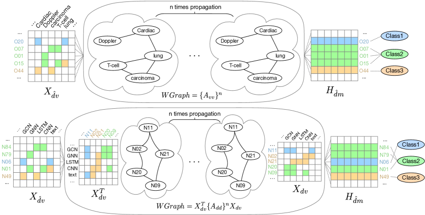
Figure 1: Schematic of WGCN model and 2 word-level graph (WGraph) calculation methods. The first row shows the word convolutional via $n$ times propagation on the WGraph $A_{vv}$ without the document correlation graph, the second row shows the word convolutional via $n$ times propagation on the document correlation graph $A_{dd}$. The subscript $d$ indicates the training documents, while $\hat{d}$ indicates another document set, which can be either training or test documents.

Building Word-level Graph: Given a corpus $D(d=|D|)$ with vocabulary size $v=|V|$, we build a flexible word-level graph (WGraph), whose nodes are all words in $V$. We consider two cases: documents are mutually independent and documents are correlated.

Documents are mutually independent. Typically, We can directly represent a word by observing whether it appears (or possibly with the term frequency) in all documents, i.e., $\vec{w_{i}}^{T}=[x_{i1},x_{i2},\cdots,x_{id}]$. Let us denote $X_{dv}$ as a document-word matrix depending on a corpus $D$ in which $i$-th column of $X_{dv}$ (denoted as $\vec{w_{i}}$) could be the presentation of $i$-th word. A correlation between two words can be calculated by a dot product between two word feature vectors i.e., $c_{ij}=\vec{w_{i}}^{T}\vec{w_{j}}$. Namely, a correlations between two arbitrary words can be defined as:

$$A_{vv}=X_{dv}^{\mathrm{T}}X_{dv}\in\mathbb{R}^{v\times v}$$ (2)

resulting in a matrix with dimensions $v\times v$. This is also a way to express the co-occurrence of words in the documents. With proper normalization, the above between-word correlation matrix $A_{vv}$ can be transformed into an adjacency matrix to build a graph. For example, a Point-wise Mutual Information (PMI, or normalized point-wise mutual information (NPMI)) matrix is one of the typical word correlation matrices to use (Yao, Mao, and Luo 2019).

Documents are correlated. By removing the prior assumption of independence, i.e. documents are correlated with some relations, for example, literature citation relations. We can define a more general word correlation matrix. Technically, the $i$-th word feature with $n$-order inter-document relationships is defined as follows:

$$\vec{w_{i}}^{(n)} =\left([x_{i1},x_{i2},\cdots,x_{id}]\underbrace{A_{dd}\cdots A_{dd}}_{\text{n times}}\right)^{T}$$ (3)

$$=\left(\vec{w_{i}}^{T}{\{A_{dd}\}}^{n}\right)^{T}$$

$n$ determines how many hops of citation relationships the word representation adopts. A bigger $n$ of $\vec{w_{i}}^{(n)}$ indicates a longer hop citation will be leveraged. Based on the order of inter-document relationship used for word representations, a general definition of word correlations is as follows:

$$A^{(m,n)}_{vv}=X_{dv}^{T}{\{A_{dd}\}}^{m}{\{{A_{dd}}^{T}\}^{n}}X_{dv}$$ (4)

where $A^{(m,n)}_{vv}$ denotes the correlations between word representations utilizing $m$-order and $n$-order inter-document relationships.

According to previous methods of GCN (Kipf and Welling 2017), $A_{dd}$ will be transformed into a symmetric Laplacian matrix , namely, $A_{dd}=A_{dd}^{T}$. Thus we can rewrite the formula in Equation 4 as follows:

$$A^{(k)}_{vv}=X_{dv}^{T}{\{A_{dd}\}}^{k}X_{dv}$$ (5)

where $k=m+n$. In the document-independent WGraph, we effectively unify both word co-occurrence ($X^{T}_{dv}X_{dv}$) and the inter-document relation information ($A_{dd}$), to make them complement each other to improve the document representation learning. In this convolution operation, the first word representation $X^{T}_{dv}$ will aggregate the relationship of the citation relationship $A_{dd}$, and then multiplied by the second $X_{dv}$ to obtain the final correlation, which means that the word co-occurrence matrix is aggregated by the citation relationship.

Word Graph Convolution: We propose a word grounded graph convolutional network (WGCN) to embed WGraph for learning document representations.

First, we apply Equation 1 on the adjacency matrix $A_{vv}$ to learn the representations of words:

$$H_{vm}=\sigma(\{A_{vv}\}^{n}X_{v}W_{0})$$ (6)

where $H_{vm}\in\mathbb{R}^{\hat{v}\times m}$ is transformed word representations with each row corresponding to a word, $\sigma$ is an activation function, and $W_{0}\in\mathbb{R}^{v\times m}$ is a weight matrix. $A_{vv}$ is a word-wise correlation matrix like in Equation 2. Since we have already involved the raw word feature matrix $X^{T}_{dv}$ to calculate $A_{vv}$ in Equation 2, here we simply set word feature matrix $X_{v}=I\in\mathbb{R}^{v\times v}$ as an identity matrix which means every word is represented as a one-hot vector to represent itself.

To predict the label of documents during testing phase, we first get the documents’ raw feature vector which could be a distribution on the whole vocabulary, e.g., term frequency vector for a document, denoted as $X_{\hat{d}v}$. Then we get the document representation by multiplying a document-word feature representation $X_{\hat{d}v}$ and the word representation vector $H_{vm}$ as below:

$$H_{\hat{d}m} =X_{\hat{d}v}H_{vm}$$ (7)

$$=X_{\hat{d}v}\sigma(\{A_{vv}\}^{n}X_{v}W_{0})$$

where $H_{\hat{d}m}\in\mathbb{R}^{\hat{d}\times m}$ and each row in $H_{\hat{d}m}$ represents a specific document. $X_{\hat{d}v}\in\mathbb{R}^{\hat{d}\times v}$ is the feature matrix of input documents. Note that $X_{\hat{d}v}$ is different from $X_{dv}$ since $X_{dv}$ is fixed as the document-word feature matrix of training documents, while $X_{\hat{d}v}$ can be the feature matrix of training or test data, which enables our model to infer representations for unseen documents.

Similar to (Wu et al. 2019), we apply a nonlinear activation function after $n$ times message propagation to simplify the model structure, resulting in a linear structure with the $n$-th power adjacency matrix as $\{A_{vv}\}^{n}$ and a single weight matrix $W$. After learning the word node embeddings in the WGraph, the document-word feature matrix of the input data $X_{\hat{d}v}$ is utilized to generate final document representations $H_{\hat{d}m}$.

As for a scenario with the provided document correlation graph, the propagation rule for the adjacency matrix $A_{vv}$ is different:

$$H_{\hat{d}m}=X_{\hat{d}v}\sigma((X_{dv}^{\mathrm{T}}\{A_{dd}\}^{n}X_{dv})X_{v}W_{0})$$ (8)

where $A_{dd}\in\mathbb{R}^{d\times d}$ is the given document correlation graph, and $X_{v}=I\in\mathbb{R}^{v\times v}$ is also an identity matrix. Only the $n$-th power of $A_{dd}$ is utilized to perform the message propagation while $X_{dv}$ does not participate in the propagation. This is done to fully leverage the pairwise information between documents in the predefined graph, for example, multiple-hop citations. Overall, our model is applicable for both without and with the document-level graph scenarios, in a sense a document-independent assumption will be a special case when $A_{vv}$ in Eq. 8 becomes an identify matrix (i.e., a matrix with diagonal elements being ones and zeros elsewhere).

For the classification task, we construct a word graph using the words in the documents. The words are connected according to their NPMI determined from the processing of the document collection. then we learn a document representation by WGCN, which is then fed into a simple MLP layer, followed by the softmax classifier to predict target labels. The loss function can be defined as:

$$\begin{split}\hat{Y}_{\hat{d}c}&=\textrm{Softmax}(\textrm{ReLu}(H_{\hat{d}m})W_{1}+b_{1})\\ \mathcal{L}&=-\sum_{i\in\hat{d}}\sum_{j\in c}Y_{i,j}\ln\hat{Y}_{i,j}\end{split}$$ (9)

where $W_{1}\in\mathbb{R}^{m\times c}$ is the weight matrix, $b_{1}\in\mathbb{R}^{c}$ is the bias, $Y$ is the label indicator matrix, $c$ is the number of classes.

Comparison with Existing Methods

In this subsection, we provide an analysis on the connection and difference of our method with existing classical methods.

First, we start to revisit our model without a given document-level graph to the following formulation:

$$\begin{split}H_{\hat{d}m}&=X_{\hat{d}v}\{A_{vv}\}^{n}X_{v}W_{0}\\ &=X_{\hat{d}v}X_{dv}^{\mathrm{T}}\{X_{dv}X^{T}_{dv}\}^{n-1}X_{dv}X_{v}W_{0}\\ &=A_{\hat{d}d}\{\hat{A}_{dd}\}^{n-1}X_{dv}W_{0}\end{split}$$ (10)

where $A_{\hat{d}d}$ is the similarity matrix between the input documents $\hat{d}$ and all training documents $d$ in corpus, $\hat{A}_{dd}=X_{dv}X_{dv}^{\mathrm{T}}$. In the formulation, we collapse the identity matrix $X_{v}$ and make a linearization of our model via removing the the only non-linear activation function similar to (Wu et al. 2019), which had proven the useless of non-linearization in information propagation.

For comparison, the linearized Text GCN model (Yao, Mao, and Luo 2019) according to (Wu et al. 2019) can be derived as:

$$\begin{split}H_{dm}&=\{\hat{A}\}^{n}X_{dv}W_{0}\\ &={\begin{pmatrix}A_{dd}&X_{dv}\\ X_{dv}^{\mathrm{T}}&A_{vv}\end{pmatrix}}^{n}X_{dv}W_{0}\\ &={\begin{pmatrix}I&X_{dv}\\ X_{dv}^{\mathrm{T}}&A_{vv}\end{pmatrix}}^{n}X_{dv}W_{0}\end{split}$$ (11)

where $\hat{A}$ is a heterogeneous graph with document and word nodes $d+v$. Moreover, the linearized GCN (Kipf and Welling 2017) model according to (Wu et al. 2019) is:

$$\begin{split}H_{dm}&=\{A_{dd}\}^{n}X_{dv}W\\ \end{split}$$ (12)

From Equation 10,11 and LABEL:eq:10, we can found that our linearized model basically has the similar convolutional formula with Text GCN and GCN models except for the adjacency matrix for information propagation. In Text GCN model, both word co-occurrence $A_{vv}$ and document-word relations $X_{dv}$ are included in the graph, while our model only keeps the former. In our method, $X_{dv}$ is decoupled from graph and directly utilized to model the document-word relations. Moreover, from Equation 10, we can explain our model from another perspective, that our model can learn representations of available documents on the inter-document graph $\hat{A}_{dd}$ derived from $X_{dv}$ with the same convolutional layer as GCN model, then effectively inference representations for unseen documents via the similarity information between available and unseen documents.

In similar way, our model with a given document-level graph can also be linearized to the following formulation:

$$\begin{split}H_{\hat{d}m}&=X_{\hat{d}v}(X_{dv}^{\mathrm{T}}\{A_{dd}\}^{n}X_{dv})X_{v}W\\ &=A_{\hat{d}d}\{A_{dd}\}^{n}X_{dv}W\end{split}$$ (13)

From Equation LABEL:eq:10 and 13, it is clear that our model has a same convolutional operation as GCN model on the document-level graph, along with the effective inductive inference mechanism via the inter-document relations $A_{\hat{d}d}$ between unseen and original documents.

Experiments

We conduct experiments on text classification with and without citation networks to evaluate our model. There are two major questions we aim to study:

1. How effective is our method in text classification without citation networks compared with existing approaches?

2. How effective is our method in text classification with citation networks the compared with existing approaches?

Text Classification without Citation Networks

We first assume that the documents are mutually independent, i.e. in the ordinary text classification datasets, there is no explicit relationship between the documents that can be used. We use the same datasets as in (Yao, Mao, and Luo 2019), including 20-Newsgroups (20NG), Ohsumed, R52 and R8 of Reuters, and Movie Review (MR). The overview of the five datasets is depicted in Table 1.

Table 1: Summary statistics of five datasets (Yao, Mao, and Luo 2019)

Dataset	Docs	Train	Test	Words	Nodes	Classes	Average Len
20NG	18,846	11,314	7,532	42,757	42,757	20	221.26
R8	7,674	5,485	2,189	7,688	7,688	8	65.72
R52	9,100	6,532	2,568	8,892	8,892	52	69.82
Ohsumed	7,400	3,357	4,043	14,157	14,157	23	135.82
MR	10,662	7,108	3,554	18,764	18,764	2	20.39

Baselines: We compare our methods with the following methods:

• CNN (Kim 2014): a CNN-based method;

• LSTM (Liu, Qiu, and Huang 2016): a LSTM-based method;

• Graph-CNN (Defferrard, Bresson, and Vandergheynst 2016): a CNN-based method with word embedding similarity graph;

• Text-GCN (Yao, Mao, and Luo 2019): a GCN-based method with a global graph for all documents and words;

• Text-GNN (Huang et al. 2019): a GNN-based method with a graph for each document. In this case, the author did not publish the source code, so we directly quote the performance in the paper;

• Fast-GCN (Chen, Ma, and Xiao 2018): a GCN-based method enhanced with importance sampling.

Experimental Settings: We set the hidden size of the convolutional layer among $\{100,200,250,500,550\}$, the dropout rate to 0.6, the learning rate among $\{0.016,0.018,0.02\}$, the window size among $\{10,20,25,50\}$, the weight decay among $\{0,5e-5\}$, the maximum training epochs with Adam to 800, the early stop epoch to 10. The parameter settings in all baseline models are the same as in (Yao, Mao, and Luo 2019; Chen, Ma, and Xiao 2018; Huang et al. 2019).

Performance: As shown in Table 2, our proposed method achieves the best performance in all datasets, which demonstrates the effectiveness of our method. When comparing with Text-GCN, our method yields around 1% improvement in the accuracy. Recall that Text-GCN builds a large graph including documents (and test documents) and word nodes, while our model builds a graph containing only word nodes. The results show that our graph can generate comparable or slightly better document representations to those generated via Text-GCN, based on the word graph where no test documents are included.

Both Fast-GCN and Text-GCN do not consider global correlations between words, which can be captured in our graph. They are unable to utilize global word correlation information. The comparison between our method and these methods show the importance of capturing global word correlations in a graph.

Note that the results of the graph-based methods tend to outperform other non-graph based methods, such as CNN, LSTM, and fastText. The reason is that the latter cannot leverage the information from a graph structure, while the graph-based methods can learn more expressive representations for nodes considering their neighborhoods.

In Table 3, we further use different order of $A_{vv}$ on the datasets of R52 and R8 to test the accuracy of our method. We choose these two datasets because other datasets will cause out of GPU memory when calculating $A^{2}_{vv}$ and $A^{3}_{vv}$. On both datasets, our method achieves the best performance when the 1-order neighborhood information in $A_{vv}$ is incorporated. With $0$-order $A_{vv}$, our method degrades to a two-layer MLP model with no neighborhood information incorporated. On the other hand, using higher-order information may over-propagate information to moderately related documents and noise can be introduced.

Table 2: Test Accuracy on document classification task for 10 times running and report mean $\pm$ standard deviation. WGCN with one convolutional layer steadily outperforms other methods on 20NG, MR, R52 and R8 based on student t-test ($p-value<0.05$). OOM: Out of GPU Memory.

Model	20NG	MR	Ohsumed	R52	R8
CNN	0.8215 $\pm$ 0.0052	0.7775 $\pm$ 0.0007	0.5844 $\pm$ 0.0106	0.8759 $\pm$ 0.0048	0.9571 $\pm$ 0.0052
LSTM	0.7318 $\pm$ 0.0185	0.7768 $\pm$ 0.0086	0.4927 $\pm$ 0.0107	0.9054 $\pm$ 0.0091	0.9631 $\pm$ 0.0033
Graph-CNN	0.8142 $\pm$ 0.0032	0.7722 $\pm$ 0.0027	0.6386 $\pm$ 0.0053	0.9275 $\pm$ 0.0023	0.9699 $\pm$ 0.0012
Fast-GCN	OOM	0.7510 $\pm$ 0.0021	0.5441 $\pm$ 0.0081	0.8515 $\pm$ 0.0045	0.9538 $\pm$ 0.0036
Text-GCN	0.8634 $\pm$ 0.0009	0.7674 $\pm$ 0.0020	0.6836 $\pm$ 0.0056	0.9356 $\pm$ 0.0018	0.9707 $\pm$ 0.0010
Text-GNN	-	-	0.6940 $\pm$ 0.0060	0.9460 $\pm$ 0.0030	0.9780 $\pm$ 0.0020
WGCN	0.8885 $\pm$ 0.0012	0.7794 $\pm$ 0.0010	0.6962 $\pm$ 0.0024	0.9486 $\pm$ 0.0009	0.9790 $\pm$ 0.0014

Table 3: Test Accuracy on document classification task for 10 times running using different order of $A_{vv}$, i.e. $A_{vv}^{k},k\in(0,1,2,3)$.

Model	R52	R8
$A_{vv}^{0}$	0.9172 $\pm$ 0.0018	0.9509 $\pm$ 0.0013
$A_{vv}^{1}$	0.9486 $\pm$ 0.0009	0.9785 $\pm$ 0.0014
$A_{vv}^{2}$	0.9062 $\pm$ 0.0012	0.9671 $\pm$ 0.0015
$A_{vv}^{3}$	0.7558 $\pm$ 0.0012	0.8995 $\pm$ 0.0018

Parameter Sensitivity: Figure 2 shows the accuracy with our model on five datasets using different hidden dimension of the convolutional layer and sliding window size in PMI calculation. We can see that: 1) On R8, R52, and Ohsumed, the test accuracy improves when the hidden dimension increases up to $250$, then it drops slowly. 2) For R8, MR and 20NG datasets, varying hidden dimension has limited influence on the test accuracy. Overall, it shows that the hidden dimension can neither be too small to embed enough information for propagation in the graph, nor too large to focus on important information for classification.

Similarly, on R8, R52, Ohsumed and MR datasets, our methods yield the best result when the window size is around 20, while smaller or larger window size can capture insufficient or noisy information. For 20NG dataset, the test accuracy consistently increases with the growing of window size. A larger window size may help capturing sufficient word correlation information with long documents, yielding better performance.

The above experiments show that the hidden dimension and window size should be chosen according to each test collection. It may not be good to use the same setting for different datasets.

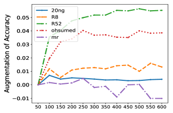
(a) hidden dimension

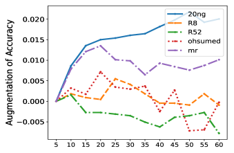
(b) window size

Figure 2: The augmentation of test accuracy with WGCN under different hidden dimension and sliding window size.

Efficiency: We further demonstrate that our method is significantly faster and has lower memory consumption compared with other GCN-based methods, with comparable and even better classification performance. The time complexity and space complexity of a one-layer GCN depend on $A_{dd}$, i.e. $O(d^{2})$, while its depend on $A_{vv}$ for a one-order WGCN, i.e. $O(v^{2})$. The difference between $O(d^{2})$ and $O(v^{2})$ is that in most cases, the vocabulary is relatively fixed, therefore $|V|$ do not grow or grows very slowly, while the dataset size ($|D|$) may be very large, and the disadvantage of GCN is that all documents must be loaded regardless of training phase or evaluation phase. We show in Table 4 the time cost and the GPU memory cost of different models on one epoch of training. We can see that WGCN has obvious advantages on both costs. In terms of time cost, Fast GCN is on average 14.6 times longer than WGCN, and Text-GCN is on average 5.1 times longer than WGCN. In terms of space cost, Fast GCN is on average 14.0 times larger than WGCN, and Text GCN is 4.5 times larger than WGCN. Notice that on the large dataset 20NG, Fast-GCN and Text-GCN models cannot be trained with GPU due to out of memory problem. Different from Fast-GCN and Text-GCN, our model removes useless nonlinear function and collapses multi-weight matrices into a single weight matrix among consecutive GCN layers. This significantly reduces both consumptions in time and memory.

Table 4: Time cost (ms) and GPU memory space cost (MiB) on one epoch of training under CUDA. (GPU: Nvidia Tesla K40c, CPU: Intel(R) 8 Core(TM) i7-2600K CPU @ 3.40GHz)

Model	20NG	MR	Ohsumed	R52	R8
	Time / Space	Time / Space	Time / Space	Time / Space	Time / Space
Fast-GCN	N/A / OOM	9,036 / 8,841	4,016 / 8,841	4,826 / 8,585	3,602 / 4,489
Text-GCN	N/A / OOM	1,060 / 3,995	4,303 / 2,960	2,365 / 2,119	1,869 / 1,613
WGCN	6,435 / 2,556	458 / 567	1,905 / 959	1,020 / 717	812 / 638

Text classification with Citation Networks

In this subsection, we present and analyze the results on the datasets in which the documents are correlated (i.e. a predefined document-level graph – the citation networks).

Datasets and Baselines: We use the same datasets as in (Kipf and Welling 2017), including Citeseer, and Pubmed citation datasets, in which a graph with the inter-document citation information is available. The overview of datasets is depicted in Table 5. We compare our method with the following methods:

1. GCN (Kipf and Welling 2017): the original transductive GCN model,

2. Fast-GCN (Chen, Ma, and Xiao 2018): an inductive GCN method which adopts importance sampling to do inference for unseen samples,

3. GIN (Xu et al. 2019): the Graph Isomorphism Network (GIN) which has a large discriminative power compared with GCNs,

4. SGC (Wu et al. 2019): a simplified linear GCN model.

Table 5: Statistics of the citation network datasets (Wu et al. 2019)

Dataset	Nodes	Edges	Classes	Train/Dev/Test Nodes
Citeseer	3,327	4,732	6	120/500/1,000
Pubmed	19,717	44,338	3	60/500/1,000

Experimental Settings: We set the hidden size of the convolutional layer to $200$, the dropout rate among $\{0.43,0.5\}$, the learning rate among $\{0.0018,0.018\}$, the weight decay among $\{0,8e-6\}$, the maximum training epoch with Adam to 1000 without early stopping. The parameter settings in all baseline models are the same as (Kipf and Welling 2017; Wu et al. 2019).

Performance: As shown in Table 6, our proposed method achieves the best performance over all baseline methods on Citeseer and Pubmed datasets. It shows that our model can be well generalized to test data using only document citation information in training data. Compared with baseline methods, besides the given citation network, our model incorporates some additional inter-document correlation information derived from document-word features and word-word graph, which could benefit our final performance.

Table 6: Test Accuracy (%) averaged over 10 runs on citation networks. WGCN steadily outperforms other methods on Citeseer and Pubmed based on student t-test ($p-value<0.05$).

Model	Citeseer	Pubmed
GCN	70.3	79.0
Fast-GCN	68.8 $\pm$ 0.6	77.4 $\pm$ 0.3
GIN	70.9 $\pm$ 0.1	78.9 $\pm$ 0.1
SGC	71.9 $\pm$ 0.1	78.9 $\pm$ 0.0
WGCN	72.2 $\pm$ 0.1	79.6 $\pm$ 0.0

In Table 7, we further present the test accuracy of our method with different orders of neighborhood information of $A_{dd}$. We can see that our method achieves the best performance when considering 1-order neighborhood information on both datasets. Considering 0-order citation information, i.e. the inter-document relationships are only calculated from document-word features, may not be sufficient for information propagation, while more than 1-order information may over-propagate to moderately related documents, resulting in worse performance in both scenarios.

Table 7: Test Accuracy (%) averaged over 10 runs on citation networks using different order neighborhood information of $A_{dd}$, i.e. $A_{dd}^{k},k\in(0,1,2,3)$.

Model	Citeseer	Pubmed
$A_{dd}^{0}$	70.5 $\pm$ 0.0	78.0 $\pm$ 0.0
$A_{dd}^{1}$	72.2 $\pm$ 0.1	79.6 $\pm$ 0.0
$A_{dd}^{2}$	67.2 $\pm$ 0.1	78.9 $\pm$ 0.0
$A_{dd}^{3}$	64.8 $\pm$ 0.1	78.4 $\pm$ 0.0

Conclusion

In this paper, we introduced a novel inductive GCN model to learn document representations in a supervised manner. The advantages of the proposed WGCN model are twofold. Firstly, WGCN degrades the document-level graph into a word-level graph, thereby reducing the complexity of the graph especially when the document number is large than the size of word vocabulary in real-world applications. As a result, the efficiency of convolution operations become much more efficient. Plus, WGCN transforms transductive learning to inductive learning, since it decouples data samples and GCN models with a document-independent graph. Therefore, WGCN can be generalized to out-of-graph documents, i.e., the documents to be classified do not need to be included in the graph when the model is trained. This is crucial for real-world applications.

Experimental results demonstrated the efficiency and effectiveness of our method along with the advantage of decoupling the data samples from the adjacency graph. For future work, it would be interesting to explore how to learn representations for documents which contain unseen words in WGraph, to cope with out of vocabulary (OOV) problem. It is also possible to extend our model to unsupervised representation learning with a large amount of unlabeled data.

References

- Bastings et al. (2017) Bastings, J.; Titov, I.; Aziz, W.; Marcheggiani, D.; and Sima’an, K. 2017. Graph Convolutional Encoders for Syntax-aware Neural Machine Translation. In Proceedings of the 2017 Conference on Empirical Methods in Natural Language Processing, 1957–1967.
- Battaglia et al. (2018) Battaglia, P. W.; Hamrick, J. B.; Bapst, V.; Sanchez-Gonzalez, A.; Zambaldi, V.; Malinowski, M.; Tacchetti, A.; Raposo, D.; Santoro, A.; Faulkner, R.; et al. 2018. Relational inductive biases, deep learning, and graph networks. arXiv preprint arXiv:1806.01261 .
- Cai, Zheng, and Chang (2018) Cai, H.; Zheng, V. W.; and Chang, K. C.-C. 2018. A comprehensive survey of graph embedding: Problems, techniques, and applications. IEEE Transactions on Knowledge and Data Engineering 30(9): 1616–1637.
- Chen, Ma, and Xiao (2018) Chen, J.; Ma, T.; and Xiao, C. 2018. FastGCN: Fast Learning with Graph Convolutional Networks via Importance Sampling. In ICLR.
- De Cao, Aziz, and Titov (2019) De Cao, N.; Aziz, W.; and Titov, I. 2019. Question Answering by Reasoning Across Documents with Graph Convolutional Networks. In Proceedings of NAACL-HLT, 2306–2317.
- Defferrard, Bresson, and Vandergheynst (2016) Defferrard, M.; Bresson, X.; and Vandergheynst, P. 2016. Convolutional neural networks on graphs with fast localized spectral filtering. In NIPS, 3844–3852.
- Hamilton, Ying, and Leskovec (2017) Hamilton, W.; Ying, Z.; and Leskovec, J. 2017. Inductive representation learning on large graphs. In NIPS, 1024–1034.
- Hochreiter and Schmidhuber (1997) Hochreiter, S.; and Schmidhuber, J. 1997. Long short-term memory. Neural computation 9(8): 1735–1780.
- Huang et al. (2019) Huang, L.; Ma, D.; Li, S.; Zhang, X.; and Houfeng, W. 2019. Text Level Graph Neural Network for Text Classification. In Proceedings of the 2019 Conference on Empirical Methods in Natural Language Processing and the 9th International Joint Conference on Natural Language Processing (EMNLP-IJCNLP), 3435–3441.
- Kim (2014) Kim, Y. 2014. Convolutional Neural Networks for Sentence Classification. In EMNLP, 1746–1751.
- Kipf and Welling (2017) Kipf, T. N.; and Welling, M. 2017. Semi-supervised classification with graph convolutional networks. In ICLR.
- Li et al. (2015) Li, Y.; Tarlow, D.; Brockschmidt, M.; and Zemel, R. 2015. Gated graph sequence neural networks. arXiv preprint arXiv:1511.05493 .
- Linmei et al. (2019) Linmei, H.; Yang, T.; Shi, C.; Ji, H.; and Li, X. 2019. Heterogeneous graph attention networks for semi-supervised short text classification. In Proceedings of the 2019 Conference on Empirical Methods in Natural Language Processing and the 9th International Joint Conference on Natural Language Processing (EMNLP-IJCNLP), 4823–4832.
- Liu, Qiu, and Huang (2016) Liu, P.; Qiu, X.; and Huang, X. 2016. Recurrent neural network for text classification with multi-task learning. In IJCAI, 2873–2879. AAAI Press.
- Lu, Du, and Nie (2020) Lu, Z.; Du, P.; and Nie, J.-Y. 2020. VGCN-BERT: Augmenting BERT with Graph Embedding for Text Classification. In Advances in Information Retrieval - 42nd European Conference on IR Research, ECIR 2020, Lisbon, Portugal, April 14-17, 2020, Proceedings, Part I, volume 12035 of Lecture Notes in Computer Science, 369–382. Springer.
- Marcheggiani and Titov (2017) Marcheggiani, D.; and Titov, I. 2017. Encoding Sentences with Graph Convolutional Networks for Semantic Role Labeling. In EMNLP, 1506–1515.
- Peng et al. (2018) Peng, H.; Li, J.; He, Y.; Liu, Y.; Bao, M.; Wang, L.; Song, Y.; and Yang, Q. 2018. Large-Scale Hierarchical Text Classification with Recursively Regularized Deep Graph-CNN. In WWW, 1063–1072.
- Scarselli et al. (2008) Scarselli, F.; Gori, M.; Tsoi, A. C.; Hagenbuchner, M.; and Monfardini, G. 2008. The graph neural network model. IEEE Transactions on Neural Networks 20(1): 61–80.
- Vashishth et al. (2019) Vashishth, S.; Bhandari, M.; Yadav, P.; Rai, P.; Bhattacharyya, C.; and Talukdar, P. 2019. Incorporating Syntactic and Semantic Information in Word Embeddings using Graph Convolutional Networks. In Proceedings of the 57th Annual Meeting of the Association for Computational Linguistics, 3308–3318.
- Veličković et al. (2017) Veličković, P.; Cucurull, G.; Casanova, A.; Romero, A.; Lio, P.; and Bengio, Y. 2017. Graph attention networks. arXiv preprint arXiv:1710.10903 .
- Veličković et al. (2018) Veličković, P.; Cucurull, G.; Casanova, A.; Romero, A.; Liò, P.; and Bengio, Y. 2018. Graph Attention Networks. In ICLR.
- Wu et al. (2019) Wu, F.; Jr., A. H. S.; Zhang, T.; Fifty, C.; Yu, T.; and Weinberger, K. Q. 2019. Simplifying Graph Convolutional Networks. In Proceedings of the 36th International Conference on Machine Learning, ICML 2019, 9-15 June 2019, Long Beach, California, USA, 6861–6871. URL http://proceedings.mlr.press/v97/wu19e.html.
- Xu et al. (2019) Xu, K.; Hu, W.; Leskovec, J.; and Jegelka, S. 2019. How Powerful are Graph Neural Networks. arXiv:1810.00826.
- Yao, Mao, and Luo (2019) Yao, L.; Mao, C.; and Luo, Y. 2019. Graph convolutional networks for text classification. In AAAI.
- Zhang, Qi, and Manning (2018) Zhang, Y.; Qi, P.; and Manning, C. D. 2018. Graph Convolution over Pruned Dependency Trees Improves Relation Extraction. In Proceedings of the 2018 Conference on Empirical Methods in Natural Language Processing, 2205–2215.