Adams et al.

Planning a Community Approach to Diabetes Care

Planning a Community Approach to Diabetes Care in Low- and Middle-Income Countries Using Optimization

Katherine B. Adams, Justin J. Boutilier, Yonatan Mintz Department of Industrial and Systems Engineering, University of Wisconsin-Madison, Madison, WI 53706, {kbadams@wisc.edu, jboutilier@wisc.edu, ymintz@wisc.edu} Sarang Deo Max Institute of Healthcare Management, Indian School of Business, Gachibowli, Hyderabad, India, 50032, sarang_deo@isb.edu

Diabetes is a global health priority, especially in low- and-middle-income countries, where over 50% of premature deaths are attributed to high blood glucose. Several studies have demonstrated the feasibility of using Community Health Worker (CHW) programs to provide affordable and culturally tailored solutions for early detection and management of diabetes. Yet, to the best of our knowledge scalable models to design and implement CHW programs while accounting for screening, management, and patient enrollment decisions have not been proposed. We introduce an optimization framework to determine personalized CHW visits that maximize glycemic control at a community-level. Our framework explicitly models the trade-off between screening new patients and providing management visits to individuals who are already enrolled in treatment. We account for patients’ motivational states (e.g., factors that influence disposition to engage in goal-directed actions), which affect their decisions to enroll or drop out of treatment and, therefore, the effectiveness of the intervention. We incorporate these decisions by modeling patients as utility-maximizing agents within a bi-level provider problem that we solve using approximate dynamic programming. By estimating patients’ health and motivational states, our model builds visit plans that account for patients’ tradeoffs when deciding to enroll in treatment, leading to reduced drop out rates and improved resource allocation. We apply our approach to generate CHW visit plans using operational data from a social enterprise serving low-income neighborhoods in urban areas of India. Through extensive simulation experiments, we find that our framework requires up to 73.4% less capacity than the best naive policy (ranking using clinical metric) to achieve the same performance in terms of glycemic control. Our experiments also show that our solution algorithm can improve upon naive policies by up to 124.5% (in terms of relative clinical performance) using the same CHW capacity.

Diabetes, Optimization, Dynamic programming, Global health

1 Introduction

As of 2021, more than 460 million people are living with diabetes globally; a number that is projected to increase by 50% in the next 20 years (Murray et al. 2020). Expanding access to diabetes screening and treatment is needed to meet the United Nations Sustainable Development Goal 3.4, which seeks to reduce premature mortality from noncommunicable diseases (NCDs) like diabetes by one third before 2030 (United Nations General Assembly 2015). Diabetes disproportionately affects low- and middle-income countries (LMICs), where it is estimated than less than one in ten people with diabetes receive guideline-based diabetes treatment (Flood et al. 2021). In addition, it is estimated that 77.2% of those with diabetes in LMICs have not achieved glycemic control (Manne-Goehler et al. 2019) and almost 90% of individuals with undiagnosed diabetes reside in LMICs (International Diabetes Federation 2021). The lack of a diagnosis often leads to poor glycemic control and, therefore, to increased risks of microvascular and macrovascular complications and mortality (Laiteerapong et al. 2019). Diabetes is a priority in urban areas in LMICs, where its prevalence is highest due to lifestyle changes driven by rapid urbanization (Ranasinghe et al. 2021).

Healthcare systems in LMICs lack the capacity required to deal with the burden of diabetes due to health workforce shortages (Scheffler et al. 2018). However, there is growing evidence that workers with shorter training and fewer qualifications such as community health workers (CHWs) can reduce the burden of diabetes through early detection (e.g., screening) and case management (e.g., treatment initiation, education, etc.), especially for populations with low health literacy, limited access to health care, and poor social determinants of health (Jeet et al. 2017, Alaofè et al. 2017, Gyawali et al. 2021). This strategy has been proposed by the global health community and is known as task shifting, i.e., redistributing tasks from highly qualified professional health workers to CHWs for managing chronic diseases like diabetes (WHO 2007). Yet, there is an urgent need for increased research to improve the design and implementation of CHW programs so that they can be efficiently and effectively scaled-up to meet population needs in the long run (WHO 2018).

Diabetes care is a challenging problem comprised of many different facets associated with detection, screening, and treatment of the disease. Due to the high rates of undiagnosed diabetes in LMICs, CHW programs must manage an explicit trade-off between providing screening visits (i.e., getting new patients on-board) and management visits (i.e., managing ongoing patients). Regarding the provision of treatment, high patient attrition rates can lead to inefficiencies in planning and capacity allocation if unaccounted for by providers (Verevkina et al. 2014, Gucciardi et al. 2008). When making treatment enrollment decisions, patients are affected by their internal motivational state, which plays an important role in initiating behaviors and selecting goal-oriented actions. Factors that can negatively impact patients’ motivational states include social stigma and cognitive burden. Social stigma can lead patients to drop out of treatment, especially when receiving CHW home visits in communities where diabetes is stigmatized (Busza et al. 2018, Nyblade et al. 2017). Similarly, the cognitive burden of treatment, which requires patients to learn how to manage their condition and implement changes in health and lifestyle behavior, may overwhelm patients and lead to drop outs (Heckman et al. 2015). Often, the effects of these adverse factors of enrollment are substantial enough to thwart potential health improvements provided by CHW interventions.

To jointly tackle the provider’s screening and management visit decisions and patient enrollment decisions, we propose a novel optimization framework for coordinating CHW visits in the context of a behavioral diabetes intervention for urban environments in LMICs. Our framework is composed of a model for how patients may enroll in the program and a dynamic programming (DP) approach for finding the optimal intervention (visit) policy. By modeling patients as utility-maximizing agents that weigh beneficial and adverse treatment factors, providers can better predict the impact of their visit plans on patient enrollment and reduce drop out rates.

In this paper, we develop an optimization framework for allocating CHW visits to patients in the context of behavioral diabetes interventions in LMICs. Through developing this framework, we provide three major contributions:

1. We extend existing models for chronic care by personalizing visits based on how patients interact with behavioral interventions delivered by CHWs (Section 4). Our modeling approach captures both the disease progression of patients and their individual enrollment decisions based on their physical health state and their motivational state. While this model has several unobserved values, we provide a machine learning method for estimating these quantities using data commonly collected by CHWs that administer these types of interventions.

2. In contrast to approaches that rely on indexability properties, we develop a DP approach that leverages the patient model to allocate CHW visits such that the number of patients that have their blood glucose levels in control is maximized (Section 5). Our model is designed for resource-constrained settings where the provider may need to trade-off managing patients that are currently enrolled and screening new patients to encourage them to join the intervention. We fully characterize the optimal policy for this model in both the single patient case and in the multi-patient resource constrained case. In the single-patient case, we establish an association between patient enrollment and glycemic control, a structure that is preserved in the multi-patient problem. Since the optimal policy in the multi-patient setting is computationally intractable, we provide an approximate DP approach that can be implemented in practice.

3. We conduct a comprehensive set of experiments that validate our modeling and optimization framework using real-world data obtained from a CHW program that operates in Hyderabad, India. In addition, we assess the generalizability of our approach using simulated patient cohorts (Section 6). Our experiments show that our solution algorithm can improve upon baseline heuristics by up to 124.5% (in terms of relative performance) using the same CHW capacity. Our approach also requires up to 61.8% less capacity than the best baseline heuristic to achieve the same performance in terms of number of patients with blood glucose in control.

2 Literature

Our work contributes to three major streams of literature: sequential resource allocation (Section 2.1), personalized healthcare (Section 2.2), and global health operations (Section 2.3).

2.1 Sequential decision-making for resource allocation

Sequential decision-making for resource allocation has been studied outside of health care for applications including retail operations (e.g., Acimovic and Graves 2015, Farias and Madan 2011), product development (e.g., Bhaskaran et al. 2021, Kornish 2001), operations scheduling/reservations (e.g., Keyvanshokooh et al. 2021, Stein et al. 2020), and machine maintenance (e.g., Glazebrook et al. 2006, Ruiz-Hernández et al. 2020). Within healthcare, authors have studied applications such as hepatitis C treatment in prisons (Ayer et al. 2019), planning community-based chronic disease care (Deo et al. 2013), hepatocellular carcinoma screening (Lee et al. 2019), breast cancer screening (Ayvaci et al. 2012), adherence to tuberculosis treatment (Mate et al. 2020, 2021), and HIV treatment under supply uncertainty (Deo et al. 2022).

There are similarities between our problem and the machine maintenance problem (e.g., machines deteriorate (disease progression) and require maintenance (management) visits). An important difference is that our setting requires modeling individual behavior (i.e., enrollment decisions) when building visit plans. Regarding healthcare applications, our work differs from prior literature in two ways. First, we explicitly model the trade-off between revisiting patients enrolled in treatment and screening new patients who are not enrolled in treatment. We note that Deo et al. (2022) also explored the trade-off in health outcomes when making operational decisions such as treatment initiation and continuity. In contrast to their work, we include a behavioral model within our resource allocation problem that accounts for patient decisions using a utility-maximizing framework. This approach accommodates not only heterogeneous patients in terms of disease progression and treatment effectiveness, but also their agency when making treatment decisions.

2.2 Personalized healthcare

Personalized healthcare allows decision-makers to tailor care while accounting for heterogeneous disease progression and treatments effects. Early work sought to improve treatment decisions and outcomes by grouping patients by health state (e.g., Deo et al. 2015), while more recent work often models disease progression and treatment effects at the individual level. For example, prior research has applied Markov decision processes to optimize personalized chronic disease screening (e.g., Skandari and Shechter 2021, Hajjar and Alagoz 2022) and multi-armed bandit models for treating multiple myeloma, type 2 diabetes, multiple sclerosis, Warfarin dosing, and physical activity interventions (Negoescu et al. 2018, Keyvanshokooh et al. 2019, Wang et al. 2019, Bastani and Bayati 2020, Mintz et al. 2020). In contrast with models that personalize care to find the best care plan for each patient individually and with a single visit type, our model solves a personalized health care problem under resource-limited settings where a provider may need to trade-off offering care for different patients due to capacity constraints$-$including trading-off screening potential new patients and managing patients who are already enrolled in treatment. Additionally, our approach considers patients’ agency, which manifests through their decisions to participate in the intervention (and impacts their outcomes).

Regarding the second point, Aswani et al. (2019) characterized patients’ responses in the context of a weight loss intervention. Similar to our approach, their framework used utility functions to model patients’ motivational states, allowing them to predict weight changes as a function of the step goals set for each individual and, therefore, set goals that optimized weight loss. Mintz et al. (2017) used a similar behavioral analytics framework for online capacitated multi-agent systems where a single coordinator provides behavioral or financial incentives for each agent using a finite budget. The coordinator’s objective depends on the states and decisions of all agents, whose utility functions are initially unknown. In contrast to their work, our setting involves more than one visit type (the equivalent of their incentive), which requires the provider to split their resources between screening and management visits. These visit decisions affect not only patients’ motivational states, but also the patient pool size that must be managed by the provider.

2.3 Global health operations

Another related stream of literature applies optimization techniques to global health in resource-limited settings (e.g., Jónasson et al. 2017, Parvin et al. 2018, Boutilier and Chan 2020, Boutilier et al. 2021b). Of particular interest is the stream of literature that applies optimization techniques to improve CHW interventions in LMICs. In this context, most prior research has focused on developing routing models to optimize CHW visits (e.g., Brunskill and Lesh 2010, Cherkesly et al. 2019). Our approach does not include routing decisions because our study setting is urban slums with high population density where CHWs walk over short distances between visits. Additionally, our intervention is planned over medium- to long-term and involves tracking patients over time to optimize their health outcomes, which are explicitly modeled in our framework.

3 Study context

In this section, we provide additional details about our problem setting that are relevant to understand the modeling assumptions made in subsequent sections.

3.1 Diabetes

Diabetes is a metabolic disorder characterized by insufficient insulin production (decline in beta-cell function) or ineffective use of insulin (insulin resistance). These issues affect the body’s ability to metabolize glucose for energy and lead to glucose accumulation in the bloodstream (Wysham and Shubrook 2020). Type 2 diabetes comprises 95% of all diabetes cases and is diagnosed by measuring the blood glucose level with one of several metrics, including random blood glucose, oral glucose tolerance test, post-prandial blood glucose, fasting blood glucose (FBG), and HbA1c.

Upon diagnosis, several strategies can be used to care for diabetes patients, including prescribing medication, educating patients, and promoting healthy lifestyle choices. Many of these measures require providing health services at the individual level, a challenging issue for healthcare systems in LMICs due to lack of capacity caused by health workforce shortages (Scheffler et al. 2018). Fortunately, some of these measures do not require medical training and can be effectively performed by CHWs (WHO 2007), who can be sought out from the communities that they will serve (allowing them to provide culturally-tailored care) and receive short training from the health system.

Patients’ motivational states can be barriers to effective treatment, affecting enrollment decisions and clinical outcomes. A patient’s motivation to enroll or stay enrolled in treatment can be affected by adverse factors of participating in the intervention, such as social stigma and cognitive burden. The use of stigmatizing phrases to describe people with diabetes has been reported in several countries and includes terms such as “sick and disabled”, “contagious”, “self-inflicting”, among others (Abdoli et al. 2018) – a depiction of the stigma that can lead patients to refuse CHW home visits (Busza et al. 2018, Nyblade et al. 2017). Therefore, CHW programs must model patient health outcomes and account for patient enrollment behavior to determine the optimal timing and type of visit to provide to each patient so that programs most effectively use their limited resources.

3.2 Diabetes in India

India is the country with the second highest burden of diabetes in the world – an estimated 74.2 million people (Lin et al. 2020), with a higher prevalence in urban than in rural areas (Ranasinghe et al. 2021). Between 2017 and 2018, the National Noncommunicable Disease Monitoring Survey (NNMS) collected data on NCD risks (including anthropometric measurements) and health-seeking behaviors from a national sample of adults from 12,000 households. Through the NNMS, researchers determined that the prevalence of type 2 diabetes and impaired FBG in India was 9.3% and 24.5% respectively. Among those with diabetes, 45.8% were aware, 36.1% were on treatment and 15.7% had their FBG in control (Mathur et al. 2022). Researchers estimate that the number of individuals with diabetes is projected to increase by 68% by 2045 and that over 53% of individuals living with diabetes are undiagnosed (International Diabetes Federation 2021).

In 2010, the Government of India launched the National Program for Prevention and Control of Cancer, Diabetes, Cardiovascular diseases and Stroke to better prepare the country for the rise in NCD prevalence. However, a recent study that included a nationally representative survey found that both private and public health facilities are not adequately prepared to handle the burden of NCDs. By assessing the availability of trained human resources, essential medicines and technologies for diabetes, cardiovascular and chronic respiratory diseases, the study found that the percentage of primary care facilities capable of managing these three NCDs varied between 1.1% in rural public to 9.0% in urban private facilities (Krishnan et al. 2021).

Regarding the economic impact of diabetes to individuals, estimates of the mean expenditure on diabetes and its complications in India range between 15,535 and 76,279 Indian Rupees (INR) (209.30-1017.05 USD) per year (Sathyanath et al. 2022, Kazibwe et al. 2021). On average, expenditures from outpatient services constituted approximately 3-5% of individual annual incomes. However, this number increased to 21% for those experiencing complications or requiring hospitalization, representing a catastrophic health expenditure (Sathyanath et al. 2022). The high out-of-pocket expenditure is explained by the high percentage of health care provided by the private sector (over 70%) (Kumar 2022) and a very small percentage of private pre-paid insurance spending (2.4%) (Dieleman et al. 2017). At a national level, researchers estimate a loss to the Gross Domestic Product of 176.6 trillion INR (2.6 trillion USD; 9.8 trillion USD in terms of purchasing power parity) due to lost productivity in 2017 alone (Banker et al. 2021).

3.3 Diabetes care provider – NanoHealth

We collaborated with and obtained data from NanoHealth, a social enterprise and former Hult Prize winner based in Hyderabad, India. Hyderabad is the capital of the state of Telangana and the fourth largest city in India with a population of 7 million (Ministry of Home Affairs 2011), including more than 1.7 million people living in 1400 urban slums (The Times of India 2012, Directorate of Economics and Statistics 2015). NanoHealth operates a diabetes screening and management program in low-income households in urban slums. The population they serve comprises individuals in the unorganized sector of the economy working as drivers, daily wage earners, domestic helpers, vendors, and self-employed professionals. The average family income of these residents ranges between 15,000 and 30,000 INR per month, which is equivalent to 200-400 USD. For reference, the average monthly family income in India is estimated to be 23,000 INR (307 USD) (Choudhury 2022).

NanoHealth employs a team of CHWs, referred to as Saathis (Hindi for companion), who are members of the communities they serve and have received basic training on diabetes care. When the data used in this paper were collected (2015-2018), NanoHealth operated in 52 urban slums (and surrounding communities) and had an average of 30 active CHWs per day. CHWs were assigned densely populated catchment areas with a population of approximately 5,000, which can be easily covered on foot to conduct both screening and management visits. Each CHW conducted an average of 144 visits per month ($\approx$5 per day) and was equipped with a “Doc-in-the-Bag” kit that included a weighing scale, measuring tape, blood glucose monitor, and blood pressure/heart rate cuffs. A mobile tablet was used to record patients’ responses to a questionnaire about lifestyle, demographics, symptoms of common ailments, and to record certain anthropomorphic measurements and vitals (Deo and Singh 2021). Screening visits were provided to identify patients with diabetes who were undiagnosed, while management visits were provided to patients who were screened, identified as high risk based on the anthropometric measurements collected, and decided to enroll in NanoHealth’s treatment program (Boutilier et al. 2021a)

4 Patient model

In this section, we describe the model of prospective and current patients’ decisions to enroll or remain enrolled in the CHW-based intervention. We assume that each patient makes these decisions based on the perceived utility (reduction in FBG) and disutility (adverse factors such as social stigma and cognitive burden weighted by their perceived importance) of staying enrolled.

Let $\mathcal{P}$ be the set of patients that can be enrolled or are already enrolled in the CHW intervention and let $i\in\mathcal{P}$ denote the index of a particular patient. Let the time index be given by $t\in\mathcal{T}=\{0,...,N\}$. We let $z_{i,t}$ indicate the enrollment status (binary) of patient $i$ at time $t$, where $z_{i,t}=1$ indicates that the patient is enrolled in the intervention. Screening visits are only conducted for patients where $z_{i,t}=0$; while management visits are only conducted for patients where $z_{i,t}=1$. At each period $t$, the provider’s decisions – whether or not to visit a patient – are denoted by the indicator variables $y_{i,t}$, which equal 1 if the provider chooses to send a CHW to visit patient $i$ at time $t$ and 0 otherwise. This variable represents a screening visit for an unenrolled patient and a management visit for an enrolled patient.

We assume that the states and actions occur in the following order. Within each period $t$, we assume that the decision to visit a patient $i$, $y_{i,t}$, precedes the patient’s enrollment decision in that same period, $z_{i,t}$. This assumption implies that the provider can affect $z_{i,t}$ through $y_{i,t}$, potentially leading patient $i$ to make a different enrollment decision within the same period. Updates to patient states occur in the following period and can be impacted by both $y_{i,t}$ and $z_{i,t}$.

We model the disease state using the log of patients’ FBG, denoted by $b_{i,t}$. We use the FBG as our primary metric because it provides a suitable trade-off between diagnostic accuracy and practical feasibility, and is the metric most commonly used in LMICs (Hoyer et al. 2018, Zhao et al. 2013). Measuring the FBG requires a fast (i.e., only water consumption) for 8 to 12 hours, which is typically done overnight. The log transform is used to capture the fact that the disease progression is proportional to the current FBG level (Derendorf and Meibohm 1999, Lee et al. 2018). We assume that $b_{i,t}$ evolves according to a set of linear dynamics of the form:

$$b_{i,t+1}=b_{i,t}+p_{i}-\mu_{i}z_{i,t}-\alpha_{i}y_{i,t}z_{i,t}+\xi_{i,t},$$ (1)

where $p_{i}$ represents the disease progression in one time period, $\mu_{i}$ represents the impact of enrollment (on FBG), $\alpha_{i}$ represents the impact of a management visit (on FBG), and $\{\xi_{i,t}\}_{t\in\mathcal{T}}$ are i.i.d disturbance terms such that $\mathbb{E}\xi_{i,t}=0$ and $\mathbb{E}\xi_{i,t}^{2}<\infty$. We assume that $p_{i}<\mu_{i}+\alpha_{i}$ to rule out the trivial case of an ineffective intervention, which does not reduce patients’ FBG. To interpret the dynamics equation, let $\tilde{b}_{i,t}=\exp(b_{i,t})$ be the true FBG. Then, we can write the dynamics as $\tilde{b}_{i,t+1}=\tilde{b}_{i,t}\exp(p_{i}-\mu_{i}z_{i,t}-\alpha_{i}y_{i,t}z_{i,t}+\xi_{i,t})$. Consider the case where $p_{i}>0$, $z_{i,t}=0$, $y_{i,t}=0$, and $\xi_{i,t}=0$, which implies that a patient’s rate of change in FBG $\tilde{b}_{i,t+1}/\tilde{b}_{i,t}$ is equal to $\exp(p_{i})$. Therefore, for an unenrolled patient whose enrollment or visit status don’t change, the rate of change in the FBG will be constant and their FBG will be equal to $\tilde{b}_{i,t+n}=\tilde{b}_{i,t}\exp(np_{i})$ after $n$ periods.

Next, we consider adverse factors experienced by enrolled patients due to either social stigma of enrollment or the cognitive burden of participation (Busza et al. 2018, Heckman et al. 2015). Let $s_{i,t}$ represent the adverse factors of enrollment experienced by patient $i$ by period $t$, and $s_{i,0}$ represent the baseline level of adversity that a patient will experience from participating in the intervention. We assume that this adversity level evolves according to the following linear dynamics:

$$s_{i,t+1}=z_{i,t}(\gamma(s_{i,t}-s_{i,0})+s_{i,0})+\beta_{i}y_{i,t}z_{i,t},$$ (2)

where $\gamma\in(0,1)$ is a discount factor on the previous period’s stigma, and $\beta_{i}>0$ is the impact on adverse factors from a management visit. Intuitively, this equation states that the adversity of a patient will increase when they are visited by a CHW, but the adverse impact of a visit will decay exponentially over time. Figure 1(a) illustrates this effect, where there is an increase in adverse factors in period 1 after a management visit is received in period 0, but eventually $s$ returns to the baseline level $s_{0}$ (in the case where no other management visits are received). The rate of exponential decay depends on $\gamma$, with lower values of $\gamma$ leading to a faster decay. We use this structure because it is reflective of how being visited by a CHW may increase social stigma as perceived by the community (Abdoli et al. 2018, Busza et al. 2018), but as time progresses, the memory (and thus the associated stigma) of the visit will fade (Ritchie et al. 2015).

(a)

(b)

Figure 1: (a) Illustration of the change in adverse factors ($s$) after a management visit in period 0 for varying $s_{0}$ and $\beta$ (for $\gamma=0.2$); (b) Illustration of the change in perceived importance of adverse factors ($\theta$) after a management visit in period 0 for varying $\theta_{0}$ and $\lambda$ (for $\rho=0.2$).

An important aspect of diabetes management is educating patients on disease progression and healthy lifestyle choices (Nazar et al. 2016). As such, we assume that a patient’s perception of the adverse factors of enrollment may decrease with the number of management visits received since enrolling in the intervention (Fisher et al. 2014). To model this, we introduce the state $\theta_{i,t}$ to represent the patient’s perceived importance of adverse factors and assume that $\theta_{i,t}$ evolves according to the following linear dynamic equation:

$$\theta_{i,t+1}=\rho(\theta_{i,t}-\theta_{i,0})+\theta_{i,0}-\lambda_{i}y_{i,t}z_{i,t},$$ (3)

where $\theta_{i,0}$ denotes the steady-state level of perceived importance of adverse factors for patient $i$, $\lambda_{i}$ denotes the decrease in the perceived importance of adverse factors that occurs each time a management visit is received as shown in Figure 1(b), and $\rho\in(0,1)$ is a discount factor on the previous period’s perception. Even though the actual adverse factors of enrollment, $s_{i,t}$, may increase when a management visit is received, we assume that the patient’s understanding of the importance of treatment and the reassurance provided by the CHWs will decrease the relevance of this factor each time a management visit is received. In the following section, the actual disutility of enrollment experienced by a patient is implemented through the product of $\theta_{t}$ (their current perceived importance of adverse factors) and $s_{t+1}$ (adverse factors of enrollment in the following period).

4.1 Patient Utility Function and Enrollment Decision

We assume that patients have knowledge of their FBG level ($b_{i,t}$), adverse factors of enrollment ($s_{i,t}$), and the perceived importance of adverse factors ($\theta_{i,t}$) when making enrollment decisions because patients’ enrollment depends on subjective notions of the utilities associated with their health and adverse treatment factors when enrolled compared to when not enrolled (Paige et al. 2016). We use this assumption to predict future patient enrollment through a framework where patients weigh the pros and cons based on the relative importance given to a potential FBG improvement (and the corresponding improvement in quality of life) at the cost of increased social stigma/cognitive burden.

Patients are also assumed to make decisions based on a myopic utility maximizing framework. Some social scientists believe that these decisions are rational with respect to heavily discounted future outcomes; an effect that has been previously observed in healthcare decision-making (Cawley 2004). Moreover, previous work (Aswani et al. 2019, Mintz et al. 2017) has shown that despite making these assumptions, resulting models still have strong predictive and prescriptive performance. Therefore, we assume that patients only consider their benefit of enrollment in the immediate next period, $t+1$, when deciding whether to enroll/stay enrolled in period $t$.

Let $\mathbb{B}:=\{0,1\}$. We denote the utility function of patient $i$ by $U_{i}:\mathbb{R}^{4}\times\mathbb{B}\mapsto\mathbb{R}$. We assume that each patient’s utility function has the structure $U_{i}=U_{i,b}+U_{i,s}$, where $U_{i,b}$ is the net utility associated with the state $b_{i,t}$ and $U_{i,s}$ is the net utility associated with the state $s_{i,t}$. Specifically, we assume that these functions are of the form:

$$U_{i,b}(b_{i,t},z_{i,t},\xi_{i,t})=-b_{i,t+1}(b_{i,t},z_{i,t},\xi_{i,t};\>y_{i,t}),$$ (4)

$$U_{i,s}(\theta_{i,t},s_{i,t+1},z_{i,t})=-\theta_{i,t}s_{i,t+1}(s_{i,t},z_{i,t};\>y_{i,t}).$$ (5)

Note that $U_{i,b}$ and $U_{i,s}$ are functions of future patient states because the patient’s decisions (and the intervention) can only impact their future states. Intuitively, $U_{i,b}$ implies that patients want to reduce $b_{i,t}$ in the future, while $U_{i,s}$ implies that patients want to reduce the adverse factors of future enrollment, scaled by their perception of the importance of the adverse factors. Thus, patients choose whether to enroll (or remain enrolled) by balancing these two parts of utility $U_{i}$.

Then, the patient’s enrollment decision at time $t$ is given by:

$$z_{i,t}\in(z_{i,t-1}+y_{i,t}-z_{i,t-1}y_{i,t})\cdot\argmax_{z\in\mathbb{B}}\ \mathbb{E}_{\xi}\ U_{i}(b_{i,t+1},s_{i,t+1},\theta_{i,t},\xi_{i,t},z).$$ (6)

Intuitively, this approach implies that a patient’s binary enrollment decision, $z_{i,t}$, maximizes their overall expected utility, where $U_{i}$ is a function of the utility associated with their future health states ($b_{i,t+1}$), adverse factors ($s_{i,t+1}$), and perception of adverse factors ($\theta_{i,t}$), where the expectation is taken over the distribution of $\xi_{i,t}$. We include the boolean “OR” operator $(z_{i,t-1}+y_{i,t}-z_{i,t-1}y_{i,t})$ to ensure that a patient’s prior enrollment status and their present enrollment decision are consistent. A patient can only choose to be enrolled in the current period if they were enrolled in the previous period or if they were not enrolled in the previous period but received a screening visit.

To characterize patients’ decisions we introduce the variable $B_{i,t}:=U_{i}(b_{i,t+1},s_{i,t+1},\theta_{i,t},\xi_{i,t},1)-U_{i}(b_{i,t+1},s_{i,t+1},\theta_{i,t},\xi_{i,t},0)$ representing the net benefit of enrollment to patient $i$. This leads to the following characterization of the patients’ enrollment decisions:

Proposition 4.1

Given the patient utility model presented by equations (4),(5),(6), and the patient state dynamic model described in Section 4, at time $t$, patient enrollment decisions are given by:

$$z_{i,t}=(z_{i,t-1}+y_{i,t}-z_{i,t-1}y_{i,t})\cdot\mathbbm{1}[B_{i,t}\geq 0],$$ (7)

where $\mathbbm{1}:\mathbb{R}\mapsto\mathbb{B}$ is an indicator function. Moreover, the benefit $B_{i,t}$ has the following closed form:

$$B_{i,t}=\mu_{i}-\theta_{i,t}(\gamma(s_{i,t}-s_{i,0})+s_{i,0})+(\alpha_{i}-\theta_{i,t}\beta_{i})y_{i,t}.$$ (8)

The complete proof of this proposition and all other theoretical results is found in Appendix 8, but we provide a brief sketch here. We can interpret the benefit of enrollment as the sum of the fixed effect of enrollment ($\mu_{i}-\theta_{i,t}(\gamma(s_{i,t}-s_{i,0})+s_{i,0})$) and the variable/visit effect ($\alpha_{i}-\theta_{i,t}\beta_{i}$). The benefit function is obtained by adding the net utility of enrollment with respect to the FBG state, $b_{i,t+1}$, and adverse factors, $s_{i,t+1}$. The equations for $b_{i,t+1}$ and $s_{t+1}$ are then used to obtain a benefit function in terms of the present states, $b_{i,t}$ and $s_{i,t}$. Note that patient enrollment requires not only the utility of enrollment to be equal to or exceed the utility of non-enrollment ($B_{i,t}\geq 0$), but also enrollment in the previous period ($z_{i,t-1}=1$) or a screening visit in the present period ($y_{i,t}=1$ if $z_{i,t-1}=0$). Also note that, although $B_{i,t}$ is the difference of two random functions, because they are both functions of the same random variable (RV) in an affine term, $B_{i,t}$ is a deterministic quantity.

Remark 4.2

According to the assumptions of the model, when $B_{i,t}=0$ the patient will be indifferent between enrolling and not enrolling in the intervention. Without loss of generality, we assume that the tie is broken in favor of enrolling in the intervention.

The characterization of patient enrollment decisions in Proposition 4.1 will later allow us to define when visiting a patient is beneficial for their enrollment and how patient enrollment relates to the optimal visit policy from the provider’s perspective.

4.2 Parameter estimation

In this section, we present a procedure that enables the provider to predict patient enrollment decisions for a proposed visit plan. At each time period, the provider observes only the enrollment status of the patient ($z_{i,t}$), a record of whether or not the patient was visited ($y_{i,t}$), and a noisy signal of the patient’s FBG – including measurement noise and biological variability in the FBG itself (Bonora and Tuomilehto 2011). Let $\bar{b}_{i,t}$ be the noisy observation of the log FBG for patient $i$ in period $t$. We assume that the relationship between $\bar{b}_{i,t}$ and $b_{i,t}$ is given by: $\bar{b}_{i,t}=b_{i,t}+\epsilon_{i,t}$, where $\epsilon_{i,t}$ are i.i.d. random variables representing the disturbance in the observations such that $\mathbb{E}[\epsilon_{i,t}]=0$ and $\mathbb{E}[\epsilon_{i,t}^{2}]<\infty$, with density function $f_{\epsilon}:\mathbb{R}\mapsto\mathbb{R}_{+}$. Note that this is a standard modeling assumption that can be satisfied by various families of distributions including Normal and Laplace distributions (Billingsley 1961). Since each patient’s parameters are estimated individually using their longitudinal visit history, we drop the patient index $i$ for the remainder of this section.

Let $\mathcal{K}\subset\mathcal{T}$ be the set of time periods for which there is an observation of the log-FBG for a particular patient. Then, we can use a maximum likelihood estimation (MLE) approach to jointly estimate all unknown model parameters, which include FBG progression ($p$), visit effect on FBG ($\alpha$), enrollment effect on FBG ($\mu$), visit effect on adverse factors ($\beta$), visit effect on perception of adverse factors ($\lambda$), and two discount factors ($\gamma$ and $\rho$). This approach also allows us to obtain FBG estimates for missing periods $t^{\prime}\in\mathcal{T}\setminus\mathcal{K}$ through the use of our state dynamics equations (1), (2), (3), and (7), an important feature for longitudinal datasets that commonly have missing data (e.g., due to a patient not being home or not being in a fasting state when a CHW visits). We show that the MLE problem can be formulated as a mixed integer linear program:

Proposition 4.3

The MLE problem (16) can be formulated as the following constrained optimization problem:

$$\underset{\mathbf{s},\boldsymbol{\theta},\beta,\alpha,\mu,p,\lambda,\rho,\gamma,\boldsymbol{\xi}}{\mathrm{minimize}}\> \sum_{t\in\mathcal{K}}\log f_{\epsilon}(\bar{b}_{t}-b_{t})+\sum_{t\in\mathcal{T}}\log f_{\xi}(\xi_{t})$$ (9a)

$$\mathrm{subject\,to}\quad b_{t+1}=b_{t}+p-\mu z_{t}-\alpha y_{t}z_{t}+\xi_{t},\quad\forall t\in\mathcal{T},$$ (9b)

$$s_{t+1}=\gamma z_{t}(s_{t}-s_{0})+z_{t}s_{0}+\beta y_{t}z_{t},\quad\forall t\in\mathcal{T},$$ (9c)

$$\theta_{t+1}=\rho(\theta_{t}-\theta_{0})+\theta_{0}-\lambda y_{t}z_{t},\quad\forall t\in\mathcal{T},$$ (9d)

$$B_{t}\geq-M(1-z_{t}),\quad\forall t\in\mathcal{T},$$ (9e)

$$B_{t}\leq Mz_{t},\quad\forall t\in\mathcal{T},$$ (9f)

$$b_{t},s_{t},\theta_{t}\geq 0,\quad\forall t\in\mathcal{T},$$ (9g)

$$\beta,\alpha,\mu,p,\lambda,\rho,\gamma\geq 0,$$ (9h)

where $B_{t}=\mu-\theta_{t}(\gamma(s_{t}-s_{0})+s_{0})+(\alpha-\theta_{t}\beta)y_{t}$ and $f_{\xi}:\mathbb{R}\mapsto\mathbb{R}_{+}$ is the density function for $\xi$ (RV).

The proof begins decomposing the likelihood function presented in 16 and subsequently applying the log to both sides, allowing the log of the products to be separated as a sum of logarithms. The term including $\bar{b}_{t}$ is then rewritten using the definition of the disturbance model and the remaining terms correspond to deterministic system dynamics. Note that this formulation is nonlinear due to the bi-linear terms in Constraints (9e) and (9f), and cannot be solved directly by commercial solvers. While standard techniques such as McCormick relaxation can be used to remove these terms, we found that using a coarse grid search to perform parameter estimation gave better results computationally. See 9 for details on our coarse grid search procedure.

5 CHW Provider Problem

In this section, we describe the dynamic programming framework used to optimize the decisions of the CHW provider (e.g., NanoHealth), while accounting for individual patient enrollment decisions. The goal of the provider is to maximize glycemic control (i.e., the number of individuals whose FBG is less than a given threshold) for the entire community under consideration. Throughout this section, we assume that the provider has full knowledge of the patient parameters described in Section 4 for all patients in the targeted community, even for those who have not been screened yet. In practice, pilot trials allow planners to obtain data that can be used as initial estimates and forecast disease progression for unscreened patients (e.g., Deo and Singh 2018).

In accordance with prevailing clinical guidelines, we define glycemic control for each patient through the use of a threshold due to a nonlinear association between FBG and the risk of complications (e.g., coronary heart disease and ischaemic stroke), with substantially higher risks for FBG levels above 125 mg/dL (WHO 2016, Emerging Risk Factors Collaboration 2010).

5.1 Single Patient Problem

To build intuition, we first consider a single-patient problem (Section 5.2 considers the multi-patient problem) and for brevity, we drop the patient index $i$. Using the dynamics described in Section 4, the state of a patient in period $t\in\mathcal{T}$ is given by $x_{t}=(b_{t},s_{t},\theta_{t},z_{t-1})$ and the provider’s action is given by $y_{t}$, which represents the decision of whether or not to visit the patient in period $t$. Let $\delta$ denote the maximum tolerable FBG. Then, the total reward is given by: $g_{t}(x_{t})=g_{t}(b_{t},s_{t},\theta_{t},z_{t-1})=\mathbbm{1}(b_{t}\leq\delta),\forall t\in\mathcal{T}.$ The total reward for a planning horizon with $N$ periods is then $\sum_{t=0}^{N}\mathbbm{1}(b_{t}\leq\delta)$. However, since $b_{t}$ is a random variable (because of dependence on $\xi$), the provider cannot diretly maximize this value and must instead maximize the expected total number of periods where the patient’s FBG is in control, which is given by $\sum_{t=0}^{N}\mathbb{E}_{\xi}[\mathbbm{1}(b_{t}\leq\delta)]=\sum_{t=0}^{N}\mathbb{P}_{\xi}(b_{t}\leq\delta)$.

Using this reward function and the patient dynamics, the optimization model to determine the optimal timing of CHW visits can be written as:

$$\underset{\mathbf{z},\mathbf{y},\mathbf{s},\boldsymbol{\theta}}{\mathrm{maximize}} \quad\sum_{t\in\mathcal{T}}\mathbb{P}_{\xi}(b_{t}\leq\delta)$$ (10a)

$$\mathrm{subject\,to}\quad \eqref{eq:mle_b_const_1}-\eqref{c_last},$$ (10b)

$$z_{t}=(z_{t-1}+y_{t}-z_{t-1}y_{t})\cdot\mathbbm{1}(B_{t}(y_{t})\geq 0),\quad\forall t\in\mathcal{T},$$ (10c)

$$y_{t},z_{t}\in\{0,1\},\quad\forall t\in\mathcal{T},$$ (10d)

where $B_{t}=\mu-\theta_{t}(\gamma(s_{t}-s_{0})+s_{0})+(\alpha-\theta_{t}\beta)y_{t}.$. The objective function maximizes the expected total number of periods where the patient’s FBG is in control (i.e., less than or equal to $\delta$).

Due to the stochasticity in the FBG update equation and the presence of bilinear terms between two continuous variables ($\theta_{t}$ and $s_{t}$) in constraints  (9e) and (9f), we leverage DP rather than standard mixed integer linear programming techniques to obtain an optimal policy. Let $V_{t}(b_{t},s_{t},\theta_{t},z_{t-1})$ for $t\in\mathcal{T}$ represent the optimal value-to-go function, i.e., the optimal expected number of periods the patient will be in control from period $t$ to period $N$. The DP equations can be written as:

$$V_{t}(b_{t},s_{t},\theta_{t},z_{t-1})= \mathbbm{1}(b_{t}\leq\delta)+$$ (11)

$$\max_{y_{t}\in\{0,1\}}\bigg{\{}\mathbb{E}_{\xi}\big{[}\,V_{t+1}\big{(}b_{t}+p-\mu z_{t}(y_{t})-\alpha y_{t}z_{t}(y_{t})+\xi_{t},z_{t}(y_{t})(\gamma(s_{t}-s_{0})+s_{0}+\beta y_{t}),$$

$$\rho(\theta_{t}-\theta_{0})+\theta_{0}-\lambda y_{t}z_{t}(y_{t}),z_{t}(y_{t})\big{)}\big{]}\bigg{\}},\forall t\in\mathcal{T}=\{0,...,N-1\},$$

$$V_{N}(b_{N},s_{N},\theta_{N}, z_{N-1})=\mathbbm{1}(b_{N}\leq\delta).$$

The value function in a general period $t$ is determined by the immediate reward for having the FBG in control in period $t$ and the expected value function in period $t+1$, where each state is updated according to the system dynamics equations explained in Section 4. In the terminal condition, the provider accrues one final reward if the FBG is in control.

5.1.1 Structural results.

In this section, we characterize the relationship between $V_{t}(b_{t},s_{t},\theta_{t},z_{t-1})$ and $z_{t-1}$ to guide the provider on how to employ visit strategies that improve glycemic control. Before we present the theorem and corresponding proof of this result, we first establish some lemmas pertaining the relationship between $z_{t}$ and $z_{t-1}$, and $V_{N}$ and $z_{N-1}$.

Lemma 5.1

$z_{t}(z_{t-1},y_{t})=(z_{t-1}+y_{t}-z_{t-1}y_{t})\cdot\mathbbm{1}(B_{t}(y_{t})\geq 0)$ is nondecreasing in $z_{t-1},\forall t\in\mathcal{T}$.

The result is obtained by evaluating the binary variable $z_{t}$ for the two possible enrollment states $z_{t-1}$. Lemma 5.1 demonstrates that, if a patient is enrolled in the intervention in period $t-1$, it is more likely they will stay enrolled in future periods irrespective of the CHW visit. Next, we consider the structure of the terminal value function.

Lemma 5.2

With probability one, $V_{N}(b_{N},s_{N},\theta_{N},z_{N-1})=\mathbbm{1}(b_{N}\leq\delta)$ is nondecreasing in $z_{N-1}$.

The proof consists of evaluating the threshold function $V_{N}$ for different values of $z_{N-1}$ and relies on the fact that, in period $N$, the value function only depends on the FBG state. Lemma 5.2 demonstrates that, if a patient is enrolled in the penultimate time period, they are more likely to have their FBG in control than if they are not. With these lemmas, we can establish our primary structural result with the following theorem, which has its proof completed by induction. The base case follows from the fact that $V_{N}(z_{N-2})$ is a composition of nondecreasing functions ($V_{N}(z_{N-1})$ and $z_{N-1}(z_{N-2})$), and therefore also nondecreasing. The induction step follows a similar process, in addition to evaluating the maximum of monotonically nondecreasing functions.

Theorem 5.3

Given the dynamic programming equations in (11), $V_{t}(b_{t},s_{t},\theta_{t},z_{t-1})$ is nondecreasing in $z_{t-1},\forall t\in\mathcal{T}$. Since $z_{t-1}\in\{0,1\}$, this is equivalent to $V_{t}(b_{t},s_{t},\theta_{t},0)\leq V_{t}(b_{t},s_{t},\theta_{t},1),\forall t\in\mathcal{T}$ with probability one.

The result above is non-intuitive because it implies that the provider should focus on keeping patients enrolled to achieve better glycemic control, even if that means that some patients should receive less visits to remain enrolled – a situation that may occur when a patient has a large increase in social stigma/cognitive burden for each visit.

5.1.2 Optimal visit policy.

We now prove structural results for the optimal CHW provider policy. Recall that patient enrollment is given by $z_{i,t}=(z_{i,t-1}+y_{i,t}-z_{i,t-1}y_{i,t})\cdot\mathbbm{1}[B_{i,t}\geq 0]$ and that Theorem 5.3 implies that a patient will never be worse off if they are enrolled in the intervention.

Theorem 5.4

Given the patient model in Section 4, a policy that solves the dynamic programming equations in (11) must satisfy the following necessary and sufficient conditions:

1. Visit the patient (i.e., $y_{t}=1$) when $z_{t-1}=1$, $B_{t}(0)<0$, and $B_{t}(1)\geq 0$ or when $z_{t-1}=0$ and $B_{t}(1)\geq 0$.

2. Never visit the patient (i.e., $y_{t}=0$) when $z_{t-1}=1$, $B_{t}(0)\geq 0$, and $B_{t}(1)<0$.

3. Indifferent between visiting and not visiting when $z_{t-1}=1$, $B_{t}(0)<0$, and $B_{t}(1)<0$ or when $B_{t}(0)\geq 0$ and $B_{t}(1)\geq 0$ or when $z_{t-1}=0$ and $B_{t}(1)<0$.

The proof of the theorem proceeds by showing that the value function is strictly increasing in $y_{t-1}$ for case $(i)$, strictly decreasing for case $(ii)$, and constant for case $(iii)$. Using the result from Theorem 5.3, which relates the value function ($V_{t}$) to the enrollment status in the previous period ($z_{t-1}$), the only remaining task is to evaluate the relationship between $z_{t}$ and $y_{t}$ (which would imply a similar relationship between $z_{t-1}$ and $y_{t-1}$). Theorem 5.4 establishes the conditions for an optimal policy. Specifically, it determines that a patient should only be visited if the visit will lead to an enrollment or prevent a patient from dropping out of treatment; that a patient should never be visited if the visit will lead them to drop out of treatment; and that a provider is indifferent if the visit cannot prevent a patient from dropping out, if a patient will remain enrolled regardless of whether a visit is received, or if an unenrolled patient will not enroll in treatment if visited.

Note that because patient decisions are outcomes of thresholding functions, and similarly, the CHW provider value function is an affine combination of thresholding functions, there may be multiple optimal policies that solve the DP equations. For example, if all patients’ FBG levels are always in control or out of control for any number of CHW visits received, it would be optimal to visit everyone, visit no one, or any other solution in-between. To choose among these optimal policies, we look ahead to the multi-patient setting where CHW resources are likely to be constrained. Hence, an advantageous characteristic of an optimal policy is to visit a patient as little as possible while ensuring they remain enrolled in the program and maintain their FBG under control. Thus, we show that the following policy is optimal:

Corollary 5.5

An optimal policy that solves the CHW provider problem described in Section 5 is given by:

$$y_{t}(x_{t})=\begin{cases}1,\>\>\text{if }B_{t}(y_{t}=1)\geq 0\text{ and }\Big{(}B_{t}(y_{t}=0)<0\\ \hskip 90.00014pt\text{ or }B_{t}(y_{t}=0)\geq 0\text{ and }\big{(}z_{t-1}=0\\ \hskip 167.00021pt\text{ or }z_{t-1}=1\text{ and }B_{t}(y_{t}=1)-B_{t}(y_{t}=0)>0\big{)}\Big{)},\\ 0,\>\>otherwise.\end{cases}$$

Clearly, the policy outlined in Corollary 5.5 meets the conditions in Theorem 5.4. Intuitively, this policy only assigns a CHW to visit a patient if the visit is necessary for enrollment or to avoid drop out, or if the visit provides a strict improvement in the patient’s utility – visiting a patient in this case can be interpreted as saving up capacity in the future by delaying the need to visit. Figure 2 provides a graphical representation of the policy structure.

Figure 2: Graphical representation of the structure of the optimal policy given in Corollary 5.5.

5.2 Multi-patient problem

In this section, we extend our results to the multi-patient problem faced by CHW organizations like NanoHealth. CHW organizations are typically resource-limited, especially those operating in global health contexts such as India. As a result, we limit the maximum number of patients that can be visited in each period; in reality, this amount can be derived from the number of CHWs and their total daily working hours. Let $C$ represent the number of available CHW visits per period. Recall that $\mathcal{P}$ represents the set of patients and note that we now add back patient indices to our variables. The multi-patient provider problem can be written as:

$$\underset{\mathbf{z},\mathbf{y},\mathbf{s},\boldsymbol{\theta}}{\mathrm{maximize}} \quad\sum_{i\in\mathcal{P}}\sum_{t\in\mathcal{T}}\mathbb{P}_{\xi}(b_{i,t}\leq\delta)$$ (12a)

$$\mathrm{subject\,to}\quad \sum_{i\in\mathcal{P}}y_{i,t}\leq C,\quad\forall t\in\mathcal{T},$$ (12b)

$$b_{i,t+1}=b_{i,t}+p_{i}-\mu_{i}z_{i,t}-\alpha_{i}y_{i,t}z_{i,t}+\xi_{i,t},\quad\forall i\in\mathcal{P},t\in\mathcal{T},$$ (12c)

$$s_{i,t+1}=\gamma z_{i,t}(s_{i,t}-s_{i,0})+z_{i,t}s_{i,0}+\beta_{i}y_{i,t}z_{i,t},\quad\forall i\in\mathcal{P},t\in\mathcal{T},$$ (12d)

$$\theta_{i,t+1}=\rho(\theta_{i,t}-\theta_{i,0})+\theta_{i,0}-\lambda_{i}y_{i,t}z_{i,t},\quad\forall i\in\mathcal{P},t\in\mathcal{T},$$ (12e)

$$z_{i,t}=(z_{i,t-1}+y_{i,t}-z_{i,t-1}y_{i,t})\cdot\mathbbm{1}(B_{t}(y_{t})\geq 0),\quad\forall i\in\mathcal{P},t\in\mathcal{T},$$ (12f)

$$B_{i,t}\geq-M(1-z_{i,t}),\quad\forall i\in\mathcal{P},t\in\mathcal{T},$$ (12g)

$$B_{i,t}\leq Mz_{i,t},\quad\forall i\in\mathcal{P},t\in\mathcal{T},$$ (12h)

$$y_{i,t},z_{i,t}\in\{0,1\},\quad\forall i\in\mathcal{P},t\in\mathcal{T},$$ (12i)

$$b_{i,t},s_{i,t},\theta_{i,t}\geq 0,\quad\forall i\in\mathcal{P},t\in\mathcal{T},$$ (12j)

where $B_{i,t}=\mu_{i}-\theta_{i,t}(\gamma(s_{i,t}-s_{i,0})+s_{i,0})+(\alpha_{i}-\theta_{i,t}\beta_{i})y_{i,t}.$ The objective function maximizes the expected total number of patient periods where FBG is in control. Constraint (12b) limits the number of visits in each period to $C$. The remaining constraints are the same as in the single patient problem, except that there is a set of constraints for each patient. Aside from constraint (12b) the problem is completely separable by patient. We exclude travel times as, in our context of densely populated urban areas, these are negligible.

Similar to the single patient problem, we leverage DP to solve the model. Let $\mathcal{V}_{t}(_{t},\mathbf{s}_{t},\boldsymbol{\theta}_{t},\mathbf{z}_{t-1})$ represent the optimal value-to-go function, where all boldface variables are vectors of length $|\mathcal{P}|$ with each entry corresponding to the state values for a given patient at time $t$ and $\odot$ represents component-wise multiplication. Furthermore, the disturbance vector $\boldsymbol{\xi}_{t}$ has independent identically distributed components with the same distribution and assumptions as $\xi_{t}$ in the previous sections. Using this notation, the DP equations are:

$$\mathcal{V}_{t}(_{t},\mathbf{s}_{t},\boldsymbol{\theta}_{t},\mathbf{z}_{t-1})=\sum_{i\in\mathcal{P}}\mathbbm{1}(b_{i,t}\leq\delta)+$$ (13)

$$\max_{\sum\limits_{i\in\mathcal{P}}y_{i,t}\leq C,y_{i,t}\in\{0,1\}}\bigg{\{}\mathbb{E}_{\boldsymbol{\xi}}\big{[}\mathcal{V}_{t+1}\big{(}_{t}+\mathbf{p}-\boldsymbol{\mu}\odot\mathbf{z}_{t}(\mathbf{y}_{t})-\boldsymbol{\alpha}\odot\mathbf{y}_{t}\odot\mathbf{z}_{t}(\mathbf{y}_{t})+\boldsymbol{\xi}_{t},\mathbf{z}_{t}(\mathbf{y}_{t})\odot(\boldsymbol{\gamma}\odot(\mathbf{s}_{t}-\mathbf{s}_{0})+\mathbf{s}_{0}+\boldsymbol{\beta}\odot\mathbf{y}_{t}),$$

$$\boldsymbol{\rho}(\boldsymbol{\theta}_{t}-\boldsymbol{\theta}_{0})+\boldsymbol{\theta}_{0}-\boldsymbol{\lambda}\odot\mathbf{y}_{t}\odot\mathbf{z}_{t}(\mathbf{y}_{t}),\mathbf{z}_{t}(\mathbf{y}_{t})\big{)}\big{]}\bigg{\}},\forall t\in\mathcal{T}=\{0,...,N-1\},$$

$$\mathcal{V}_{N}(_{N},\mathbf{s}_{N},\boldsymbol{\theta}_{N},\mathbf{z}_{N-1})=\sum_{i\in\mathcal{P}}\mathbbm{1}(b_{i,N}\leq\delta).$$ (14)

5.2.1 Optimal visit policy.

To obtain structural results for the optimal visit policy of the multi-patient problem, we first use the optimal policy from the single-patient problem to define a set that represents the patients that would be visited in each period if there was no capacity constraint. To build intuition for why this would be of interest, consider the case when the multi-patient problem is uncapacitated, that is $C\geq|\mathcal{P}|$. In this case, the problem is completely separable by patient and can thus be decomposed into $|\mathcal{P}|$ single patient problems that can be solved using the results in Section 5.1. Thus, in this case, we would only visit patients if we visit them in the single patient setting. We call this group of patients the set of patients of interest.

Definition 5.6

Let $\mathcal{I}_{t}$, the set of patients of interest in period $t\in\mathcal{T}$, be defined as:

$$\mathcal{I}_{t}:=\Bigg{\{}i\in\mathcal{P}\;\Big{|} \big{(}B_{i,t}(y_{i,t}=1)\geq 0\big{)}\text{ and }$$

$$\big{(}(B_{i,t}(y_{i,t}=0)<0)\>\text{ or }\>(z_{i,t-1}=0)\text{ or }(z_{i,t-1}=1\text{ and }B_{t}(y_{t}=1)-B_{t}(y_{t}=0)>0)\big{)}\Bigg{\}}.$$

In the constrained case (i.e., $C<|\mathcal{P}|$), we prove that an optimal policy to the multi-patient problem can be obtained by appropriately choosing $C$ patients from $\mathcal{P}$ by identifying $\mathcal{I}_{t}$. The conditions for inclusion in $\mathcal{I}_{t}$ are derived directly from Corollary 5.5 and, for the single patient problem, $y_{t}=1$ if $\mathcal{I}_{t}$ is non-empty. For notational brevity, let $V_{i,t}^{j}=\mathbb{E}_{\boldsymbol{\xi}}\big{[}\mathcal{V}_{i,t}(b_{i,t},s_{i,t},\theta_{i,t},z_{i,t-1}(y_{i,t-1}=j))\big{]}$ and $\mathcal{I}_{t}^{j}=\{i\in\mathcal{I}_{t}|y_{i,t}=j\}$ where $j\in\{0,1\}$.

Our main result related to the structure of the multi-patient provider problem (Theorem 5.10) is non-trivial to derive and requires the use of several auxiliary results. First, we prove the following lemma regarding the one stage problem (i.e., $t=N-1$).

Lemma 5.7

For period $N-1$, an optimal visit policy is given by visiting all patients in set $\mathcal{S}_{N-1}\subset\mathcal{I}_{N-1}$ where $\mathcal{S}_{N-1}:=\{i\in\mathcal{I}_{N-1}:y^{*}_{i,N-1}=1\}$ where $\mathbf{y}^{*}_{N-1}$ is defined as:

$$\mathbf{y}^{*}_{N-1} \in\argmax_{\{i\in\mathcal{I}_{N-1}|\sum_{i\in\mathcal{I}_{N-1}}y_{i,N-1}\leq C\}}\Bigg{(}\sum_{i\in\mathcal{I}^{1}_{N-1}}V_{i,N}^{1}+\sum_{i\in\mathcal{I}^{0}_{N-1}}V_{i,N}^{0}\Bigg{)}.$$

Note that $y_{N-1}$ can only affect the value function in period $N$, and that $\mathcal{V}_{N}$ depends solely on the FBG, which is additively decomposable by patient per Equation (14). The proof is then completed by considering two cases: $|\mathcal{I}_{t}|\leq C$ and $|\mathcal{I}_{t}|>C$. The proof of the first case follows directly from Theorem 5.3 and Corollary 5.5, and the second case is shown through a proof by contradiction that uses an exchange argument. Essentially, Lemma 5.7 establishes that our desired policy structure is optimal in the single-stage problem (and thus the final period of the dynamic programming algorithm). Although this result is trivial, it is not obvious that this structure will hold for all periods in the planning horizon. Any effects of $\mathbf{y}_{N-1}$ on adverse factors of enrollment ($\mathbf{s}_{N}$) or on the enrollment itself ($\mathbf{z}_{N}$) would not impact the FBG (nor the provider reward) by period $N$, but earlier visit decisions $\mathbf{y}_{t}$ for $t<N-1$ could affect the FBG directly and indirectly through effects on $\mathbf{s}_{t+1}$ and $\mathbf{z}_{t+1}$. Because of the capacity constraint, this means that improperly allocating a visit in a current period to a patient that would be enrolled without a visit could lead a different patient to require a future visit to maintain their enrollment status. Thus miss-allocating capacity in an earlier period could mean dedicating future capacity to patients that would otherwise not need it. This means that potentially the value functions of the patients cannot easily be decomposed due to this entanglement. Counter intuitively, our next result shows that the value functions in the multi-patient multi-period problem are also additively decomposable.

Proposition 5.8

For all $t<N$ the joint value function $\mathcal{V}_{t}(_{t},\mathbf{s}_{t},\boldsymbol{\theta}_{t},\mathbf{z}_{t-1})$ is additively decomposable by patients. That is, at each time $t$ and for each patient $i\in\mathcal{P}$ there exist patient component functions $\mathcal{V}_{i,t}(b_{i,t},s_{i,t},\theta_{i,t},z_{i,t-1})$ such that: $\mathcal{V}_{t}(_{t},\mathbf{s}_{t},\boldsymbol{\theta}_{t},\mathbf{z}_{t-1})=\sum_{i\in\mathcal{P}}\mathcal{V}_{i,t}(b_{i,t},s_{i,t},\theta_{i,t},z_{i,t-1})$.

The proof is completed by induction. For the base case (period $N-1$), the dynamic programming equations in 13 and Lemma 5.7 yield the desired form. Proving the induction step requires evaluating the maximum over the sum of expected value functions $\mathcal{V}_{i,t+1}$ over the set of patients $\mathcal{P}$. If the optimal solution is to visit no patients or all patients, the proof is trivial. If the optimal solution is to visit a proper subset of patients, the induction step proof follows a similar argument to the base case – identifying partitions of $\mathcal{P}$ and rewriting the definition of $\mathcal{V}_{i,t}$ using summations only.

Lemma 5.7 and Proposition 5.8 show that the joint value function $\mathcal{V}_{t}(_{t},\mathbf{s}_{t},\boldsymbol{\theta}_{t},\mathbf{z}_{t-1})$ can always be decomposed additively into patient-wise components. That is $\mathcal{V}_{t}(_{t},\mathbf{s}_{t},\boldsymbol{\theta}_{t},\mathbf{z}_{t-1})=\sum_{i\in\mathcal{P}}\mathcal{V}_{i,t}(b_{i,t},s_{i,t},\theta_{i,t},z_{i,t})$ for all $t\in\mathcal{T}$. These auxiliary results will eventually allow us to interpret Theorem 5.10 as providing an optimal solution that finds optimal sets of patients belonging to $V^{0}$ and $V^{1}$ at each time period, with patients potentially switching between these sets throughout the planning horizon. Proposition 5.8 holds because the provider rewards are a function of the patient enrollment states, which are binary – a structure that originates directly from the problem setting being studied. To prove Theorem 5.10, our remaining intermediate step is to show that each of the patient component value functions $\mathcal{V}_{i,t}$ is nondecreasing in the enrolment state $z_{i,t-1}$.

Proposition 5.9

For all $t<N$ and for each $i\in\mathcal{P}$ the component value functions $\mathcal{V}_{i,t}(b_{i,t},s_{i,t},\theta_{i,t},z_{i,t-1})$ are nondecreasing in $z_{i,t-1}$.

The proof is completed by induction. The base case relies on defining the component value functions in a manner similar to the proof of Proposition 5.8 and using Lemma 5.1 and Lemma 5.2. The induction step is completed by using Lemma 5.1 and the induction hypothesis. The result of this proposition shows that the structure of the multi-patient problem is similar to that of the single patient, in that we ought to increase the amount of time an individual is enrolled in the program in order to maximize the value-to-go. Now we can proceed to show the optimal policy for the multi-patient problem, which is:

Theorem 5.10

In the multi-patient multi-period problem, an optimal policy is given by visiting all patients in the set $\mathcal{S}_{t}\subset\mathcal{I}_{t}$, where $S_{t}=\{i\in\mathcal{I}_{t}:y^{*}_{i,t}=1\}$ and

$$\mathbf{y}^{*}_{t}\in\argmax_{\Big{\{}i\in\mathcal{I}_{t}\Big{|}\sum\limits_{i\in\mathcal{I}_{t}}y_{i,t}\leq C\Big{\}}}\Bigg{(}\sum_{i\in\mathcal{I}^{1}_{t}}V^{1}_{i,t+1}+\sum_{i\in\mathcal{I}^{0}_{t}}V^{0}_{i,t+1}\Bigg{)}.$$ (15)

Intuitively, Theorem 5.10 states that in the multi-patient setting, only patients from the set $\mathcal{I}_{t}$ should be visited. Moreover, if $|\mathcal{I}_{t}|>C$, then ties should be broken by selecting patients with larger value-to-go functions when visited. Ties may be present due to the value functions being functions of enrollment, which is binary valued. The proof of Theorem 5.10 focuses on the constrained case where $|\mathcal{P}|>C$ since the unconstrained case follows directly from Corollary 5.5. First, we consider the case where $|\mathcal{I}_{t}|\leq C$. Then, by way of contradiction we assume that a visit is allocated for a patient $j\notin\mathcal{I}_{t}$, and using the definition of $\mathcal{I}_{t}$, Proposition 5.9, and Lemma 5.1 we reach the contradiction. For the case where $|\mathcal{I}_{t}|>C$, the proof is completed by contradiction using an exchange argument, following a similar process to the proof of Lemma 5.7. See Appendix 8 for more details.

5.2.2 Implementation of the optimal visit policy.

To solve the multi-patient problem, we implement a solution approach that we refer to as the Enrollment Algorithm (EA). We use this approach because it is very challenging (computationally) to exactly evaluate the value function $\mathcal{V}_{i,t}(b_{i,t},s_{i,t},\theta_{i,t},z_{i,t-1})$ for every patient $i$ and time period $t$, as would be needed to implement Theorem 5.10 exactly. Instead, because Theorem 5.10 proved that the optimal set of patients to visit at each period ($\mathcal{S}_{t}$) is a subset of the set of patients of interest ($\mathcal{I}_{t}$), we estimate $\mathcal{S}_{t}$ using a subset of $\mathcal{I}_{t}$ obtained by ranking patients using several criteria.

Intuitively, the EA incorporates the results from Corollary 5.5 to first identify $\mathcal{I}_{t}$ for each period $t$ (see Figure 2 for a graphical representation of the conditions defining $\mathcal{I}_{t}$). If $|\mathcal{I}_{t}|\leq C$, then we set $y_{i,t}=1\>\forall i\in\mathcal{I}_{t}$. If $|\mathcal{I}_{t}|>C$, then we use one of four tie-breaking rules to rank the patients and select the first $C$ patients to be visited. The four tie-breaking rules used to sort patients $i\in\mathcal{I}_{t}$ (and the intuition behind them) are:

1. EA Ascending FBG: Order patients by ascending $b_{i,t}$. The provider may have more patients with their FBG in-control if they focus on patients with lower FBG (easier to control).

2. EA Descending FBG: Order patients by descending $b_{i,t}$. The provider may have a greater impact if they can flip patients with high FBG from out of control to in-control, especially when the patients with lower FBG have slow disease progression (in-control even if unvisited).

3. EA Descending value-to-go: Estimate the value-to-go of each patient by solving a single-patient problem using the one-step look-ahead policy that is based on Corollary 5.5. Order patients by descending value-to-go. The value-to-go for each patient is determined based on the number of periods that the patient would have their FBG in control if we were to implement the optimal policy for a single-patient problem, that is, $\tilde{\mathcal{V}}_{i,t}=\sum\limits_{t^{\prime}\in\mathcal{T}|t^{\prime}\geq t}\mathbbm{1}(b_{i,t^{\prime}}\leq\delta)$. The provider chooses the patients that would have a greater number of periods in control in the single patient problem.

4. EA Descending value-to-go/visits: Estimate the value-to-go and the number of visits required in the remaining periods for each patient by solving a single-patient problem. Order patients by descending ratio of value-to-go divided by the number of visits, $\tilde{\mathcal{V}}_{i,t}/L_{i,t}$. We calculate the number of visits ($L_{i,t}$) that the patient would require from the present period until the end of the horizon under the optimal single-patient problem policy, that is, $L_{i,t}=\sum\limits_{t^{\prime}\in\mathcal{T}|t^{\prime}\geq t}y_{i,t^{\prime}}$. The provider divides the total number of periods in control for each patient by the number of visits required to obtain a ratio (i.e., return/cost). The ratios are then ranked in descending order.

6 Numerical Experiments

In this section, we describe the data and experimental setup used to evaluate our approach. Section 6.1 describes the overall simulation framework including how we incorporated uncertainty in disease progression, the baseline approaches used for comparison, and the evaluation metrics used. Section 6.2 presents the results from simulations performed with NanoHealth’s data. Section 6.3 describes how we generated artificial patient cohorts, which we refer to as expanded scenarios, to evaluate the generalizability of our approach, and Section 6.4 presents the results from the expanded scenarios. Finally, Section 6.5 describes broad managerial implications obtained through our experiments.

6.1 Simulation framework

In all experiments, we solve the multi-patient CHW visitation problem described in Section 5 using a planning horizon of $N=60$ periods, corresponding to five years of monthly visits (in line with NanoHealth operations). We conducted simulations for capacity levels ranging from 5% to 100% in 5% increments, where the capacity level is expressed as a percentage of the per period visit capacity ($C$) divided by the number of patients in the community being served ($|\mathcal{P}|$). All simulations were run using Python 3.7 on a PC with 16 GB of RAM and an Intel Core i5 processor.

6.1.1 Data.

Our dataset includes anonymous longitudinal data about a patient cohort treated by NanoHealth, which includes 378 patients that received at least six visits through NanoHealth’s intervention in Hyderabad, India. For each patient, our data includes an FBG reading each time they were visited by a CHW (for both screening and management visits).

6.1.2 Uncertainty in disease progression.

We simulated $\xi_{i,t}$ as normally distributed with mean zero and standard deviation $\sigma$, where $\sigma$ was estimated using historical data from NanoHealth by calculating the sample standard deviation of the change in FBG between successive periods across all patients. We solve 10 replications of each instance each with a different random seed.

6.1.3 Baseline heuristics.

We use four naive baseline heuristics as benchmarks:

• Visit No One: No patients are visited during the planning horizon.

• Visit Everyone: Every patient is visited at every period.

• Descending FBG: Visit $C$ patients ranked by descending FBG.

• Ascending FBG: Visit $C$ patients ranked by ascending FBG.

Note that the last two baseline heuristics differ from their EA counterparts in that patients are not filtered by identifying set $I_{t}$ prior to ranking in each period $t$.

6.1.4 Evaluation metrics.

To compare our solution algorithms, we introduce the concept of patient-periods in control (PPC), i.e., the number of patients with their FBG in control (under the threshold $\delta$) at the end of each period. By computing the total number of PPC across all periods, we can easily compare the relative performance of each heuristic for the full planning horizon. We also compare our algorithms using the number of screening visits, total enrollment, and FBG.

6.2 NanoHealth Case Study

In this section, we describe the experiments and results using a real patient cohort. To obtain personalized patient parameters required to solve the multi-patient provider problem, we first solved the parameter estimation problem described in Section 4.2 for each patient using their actual visit history. See Appendix 10 for details. According to the parameter estimation results, there were four distinct clusters present in NanoHealth’s cohort, indicating that there is significant heterogeneity in patient parameters (e.g., disease progression, enrollment effect, visit effect). Our NanoHealth simulation results indicate that visit allocation decisions and glycemic control are both improved through a planning approach that models individual patient decisions.

6.2.1 PPC performance.

Figure 3(a) shows box and whisker plots of PPC for each algorithm when the visit capacity per period corresponds to 45% of the total number of patients in the cohort. We chose this capacity level because we observe the largest divergence in PPC performance across the different algorithms. We observe that EA with Descending FBG achieves the best performance with a PPC of 42.1%, followed by EA Ascending FBG with a PPC of 40.6%. These algorithms have a relative improvement upon the best benchmark heuristic (Descending FBG) of 9.8% and 5.8%, respectively.

Figure 3(b) shows the PPC at varying capacity levels in 5% increments. We observe that the different algorithms are comparable up until about 20% capacity (excluding the benchmarks Visit No One and Visit Everyone). As the capacity increases, the EA with Descending FBG has the fastest gain in performance, reaching a 9.8% better performance at 45% capacity with respect to the best benchmark heuristic. Furthermore, to achieve 40% PPC, the EA with Descending FBG requires 34.3% capacity, while the Descending FBG heuristic requires 59.5% capacity, a 25.2% absolute (73.4% relative) difference.

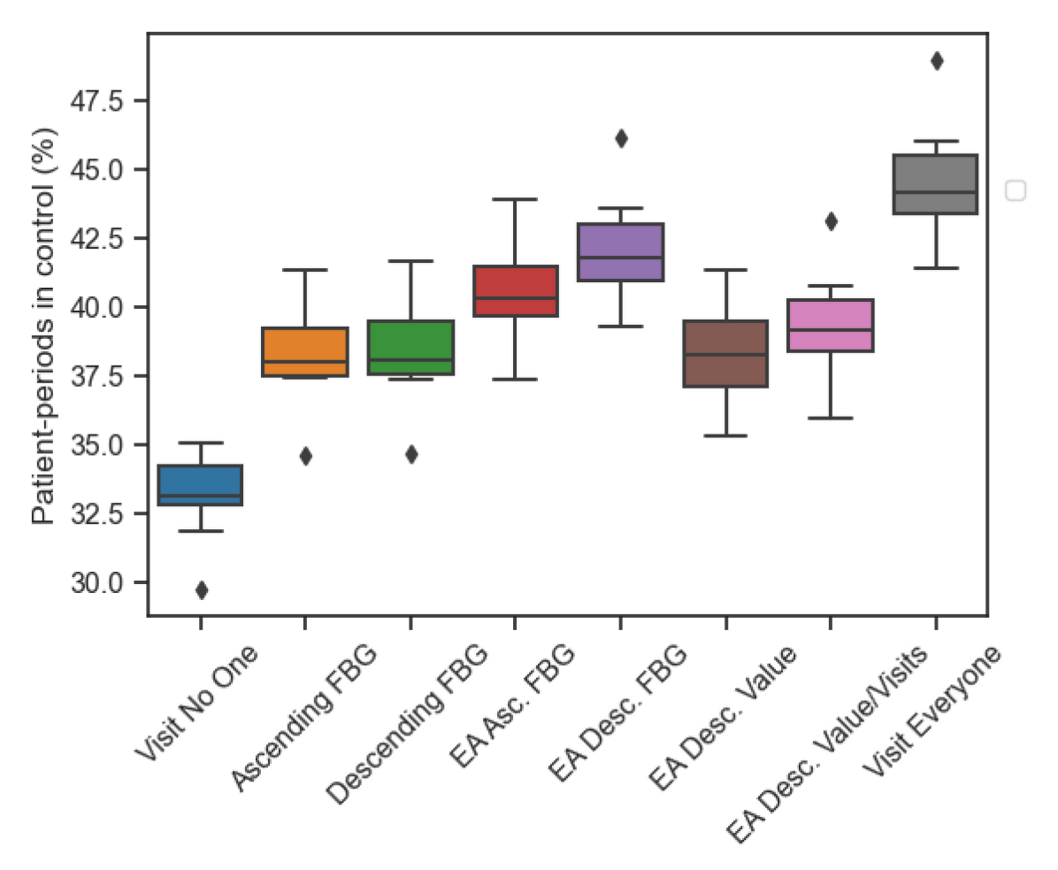
(a)

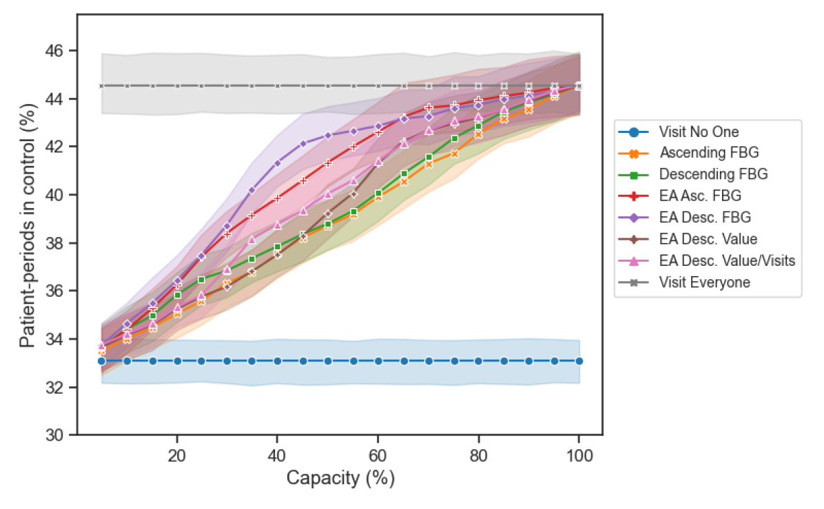
(b)

Figure 3: (a) Boxplots showing the interquartile range of PPC for each heuristic at 45% capacity; (b) Line graph of PPC for each heuristic for varying capacity levels (5% increments) with shaded 95% confidence intervals.

6.2.2 Visit types and patient enrollment.

Figure 4 illustrates the long-term patterns in screening and patient enrollment. Figure 4(a) displays the proportion of CHW visits that were screening visits across the planning horizon. The first 10 periods in the planning horizon are not shown since the short-term screening patterns are similar for all heuristics. We observe that the EA implementations have a lower percentage of visits that are dedicated to screening, in addition to a periodic pattern with the screening visits reaching 0% in some periods, then increasing, then returning to 0%. This suggests that some patients may drop out of treatment and require additional screening visits to re-enroll. Furthermore, we observe that the benchmark heuristics (Descending FBG and Ascending FBG) maintain a higher overall percentage of screening visits. However, Figure 4(b), which shows the proportion of enrolled patients, demonstrates that these two benchmark heuristics also have the lowest percentage of patients enrolled in treatment during most of the planning horizon. Intuitively, these results suggest that the screening visits conducted by the benchmark heuristics are not allocated as efficiently as the screening visits conducted by the EA implementations. In fact, the enrollment for the Descending FBG and Ascending FBG heuristics never surpasses 81% and 93%, respectively, while all EA implementations maintain enrollment above 90%, with three of them approaching 100%.

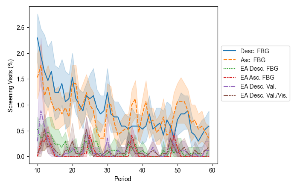
(a)

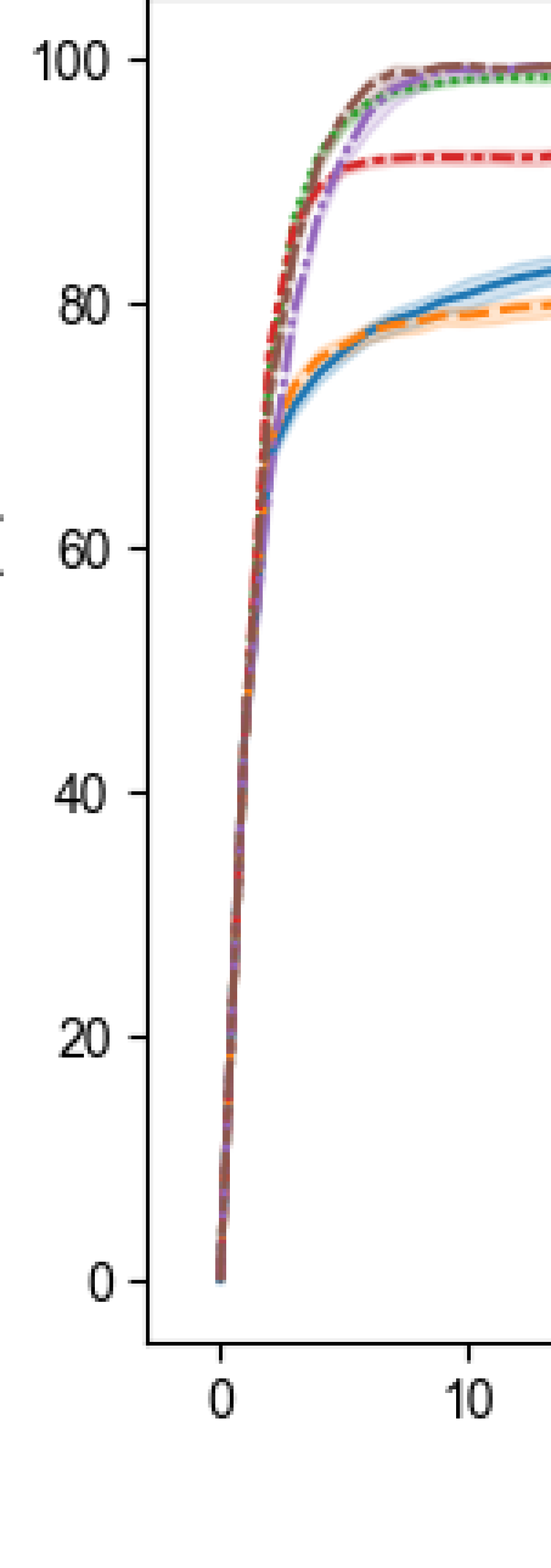
(b)

Figure 4: (a) Line graph showing the proportion of CHW visits that were screening visits at 45% capacity with shaded 95% confidence intervals starting at period 10; (b) Line graph showing the proportion of patients enrolled in treatment at 45% capacity with shaded 95% confidence intervals.

6.2.3 FBG distribution.

Figure 5 shows violin plots with the distribution of log-FBG levels at the end of the planning horizon. The Visit No One benchmark shows a bimodal distribution due to the fast FBG increase experienced by some patients, and slow increase or stabilization in FBG experienced by other patients, leading to two distinct peaks. Because we modeled disease progression proportionally to current FBG levels, an artifact of our model is that some patients present extremely high FBG levels that would not occur in practice. In these cases, life-threatening conditions would likely occur before those FBG levels are reached. In terms of numerical results, the Visit No One policy achieves a median and 90th percentile log-FBG of 16.6 and 422.1, respectively. Although the EA heuristic with Descending value-to-go/visits has a similar shape with a long tail, the median and 90th percentile are 5.2 and 33.5 (relative improvements of 68.7% and 92.1%), respectively. In contrast, Descending FBG and EA Descending FBG were able to improve the 90th percentile to 29.2 and 28.3 (relative improvements of 93.1% and 93.3%), respectively. Although Descending FBG and EA Descending FBG have similar shape, EA Desc. FBG has a median and 90th percentile FBG that is 32.5% and 3.1% lower than Desc. FBG, respectively. Note that the EA Desc. Value-to-go/Visits and EA Desc. FBG achieve comparable medians (6.9 and 5.2, respectively), and that the former has a higher 90th percentile (33.5) compared to the latter (28.3), suggesting that the EA Desc. FBG provides visits to a greater proportion of patients.

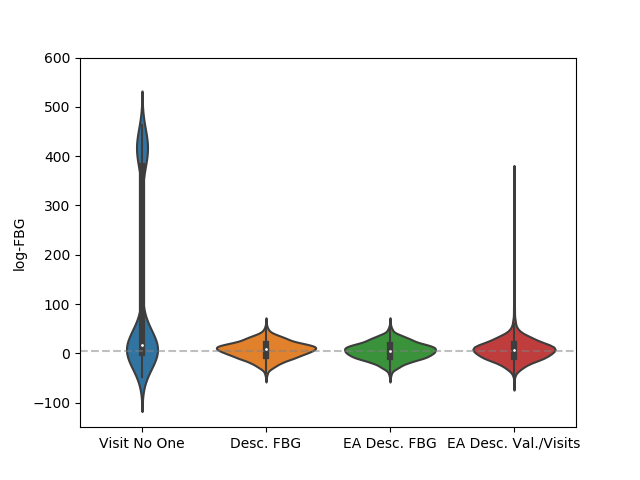
Figure 5: Violin plots showing the distribution of log-FBG values at the end of the planning horizon for NanoHealth’s patient cohort at 45% capacity. The white dots, bold line, and thin line indicate the median, interquartile range (IQR), and 1.5 times the IQR for each violin plot, respectively. The FBG threshold $\delta$ is indicated by a horizontal gray dashed line.

6.3 Expanded Scenarios’ Setup

We evaluate the generalizability of our approach through simulation experiments with expanded scenarios (i.e., artificial patient cohorts) that have varying patient parameters. For each scenario, we evaluate the performance of the four EA implementations (described in Section 5.2.2) and the four baseline heuristics (described in Section 6.1.3). To generate the scenarios, we first created five patient groups derived from observations of real world data and conversations with our collaborator – specifically, each group is represented by a “patient-type” that includes seven parameters (see Table 4). The five groups (A, B, C, D, and E) have their parameter centroids represented in Figure 6. We combined two patient types per scenario, totalling 10 scenarios with 50% of patients from each group. After extensive computational experiments, we picked a subset of two illustrative scenarios. We also built a scenario with 20% of patients from each group. Figure 7 provides a graphical representation of the composition of the three scenarios using the patient groups.

Figure 6: Visualization of the group centroids used in truncated normal sampling procedure.

We build each scenario (i.e., artificial community) in three steps. First, we sample the patient state dynamics parameters from each group described in Table 4. Patient parameters are assumed to be independent and to have constant variance across different groups, therefore only the mean vector differs for each group and the parameters can be sampled using truncated normal distributions. We use a lower bound of zero for the truncation based on the assumption that the parameters being sampled are non-negative. Second, we set the discount factors, $\rho_{i}$ and $\gamma_{i}$, to 0.2 for all patients $i\in\mathcal{P}$ in all scenarios because the majority of real world patients had $\rho=\gamma=0.2$ after solving the parameter estimation problem in Section 4.2 (over 93% and over 95% for $\rho$ and $\gamma$, respectively). Recall that both $\gamma$ and $\rho$ are contained in the interval $(0,1)$, where 0 indicates that a state immediately returns to its steady state level ($s_{i,0}$ and $\theta_{i,0}$ for $s_{i,t}$ and $\theta_{i,t}$, respectively), while 1 indicates that state at time $t$ is fully determined by the immediate prior state ($s_{i,t-1}$ and $\theta_{i,t-1}$), with the addition or subtraction of $\beta_{i}$ or $\lambda_{i}$ in the case of an increase in adverse factors or a decrease in perception of adverse factors, respectively. The empirical results indicate that most patients tend to quickly return to their steady-state levels of $s_{i,0}$ and $\theta_{i,0}$. Third, we sample initial FBG values (i.e., $b_{i,0}$) using a normal distribution fit to the initial FBG values from the NanoHealth cohort. We confirmed that initial FBG was approximately normally distributed using a Kolmogorov–Smirnov at a significance level of 0.05.

Figure 7: Graphical illustration of the composition of the artificial scenarios.

6.4 Expanded Scenarios’ Results

This section presents results for the experiments that use artificial patient cohorts. Section 6.4.1 compares PPC at varying capacity levels, Section 6.4.2 explores the breakdown of visit types and patient enrollment for the planning horizon, and Section 6.4.3 compares heuristic approaches with respect to the final log-FBG distribution. Our scenario simulation results show that the EA Descending Value-to-go/Visits implementation outperforms all other approaches in terms of PPC performance at most capacity levels for all scenarios, and that the EA Descending FBG maintains a competitive PPC performance whilst maintaining higher enrollment and visit equity.

6.4.1 PPC performance.

Figure 8 shows three plots (one per scenario) with the percentage of patient-periods in control (PPC) as a function of capacity. Recall that the capacity is expressed as a percentage representing the number of visits available per period divided by the total number of people in the community. In all scenarios, the best EA implementation outperforms ranking by Ascending FBG and Descending FBG (baseline heuristics) for capacities up to 65%. In Figure 8(c), the EA Descending value-to-go/visits achieves 124.5% greater PPC relative to the Ascending FBG heuristic for the same capacity level (5%). In all scenarios and at most capacity levels, the EA Descending value-to-go/visits implementation has a superior performance to the others. Alternatively, we can can compare the capacity required for the best naive heuristic to perform comparably to the best EA implementation. For example, Figure 8(c) shows that to achieve a performance of approximately 30% of PPC, the EA with Descending Value-to-go/Visits requires a capacity of 18.7%, while a capacity of 49.0% (161.5% greater) is required to achieve the same performance with the best naive heuristic (Ascending FBG). The consistently high performance of the EA Descending Value-to-go/Visits across scenarios shows that it provides a better value-to-go approximation for all patients ($\mathcal{V}_{t}$). Even though $\mathcal{V}_{t}$ was approximated using value functions for single-patient problems, the superior performance of this EA implementation makes sense due to our result pertaining the additivity of $\mathcal{V}_{t}$ into “component value functions” (see Theorem 5.10).

By analyzing Figure 8 across different scenarios, we note that the EA Ascending FBG and Ascending FBG have a superior performance to their counterparts (EA Descending FBG and Descending FBG) at lower capacities, which suggests that when the capacity is highly constrained, the PPC performance can be improved the most by focusing on patients with the lowest FBG levels (easier to maintain in control). This effect is clear for scenarios where patients have a fast disease progression (e.g., scenario 2). Also note that EA Ascending FBG and Ascending FBG have a comparable performance for scenario 2, whereas EA Ascending FBG performs significantly better for scenarios 1 and 3. This phenomenon is explained by the fast disease progression ($p$), moderate enrollment effect ($\mu$), and high increase in adverse factors ($\beta$) for both groups that compose scenario 2 (B and D). Because $\mu<p$, being enrolled is not enough to deter the disease progression for these patients. Management visits have to be planned carefully to improve PPC while avoiding drop outs due to the high $\beta$, which the EA Ascending FBG accomplishes by filtering the patients of interest at each period prior to ranking by ascending FBG. In addition to reducing drop out rates, our EA implementations seek to allocate limited resources efficiently by visiting an enrolled patient who would not drop out if unvisited only if it provides a strict increase in their benefit function (see Theorem 5.4 and Corollary 5.5).

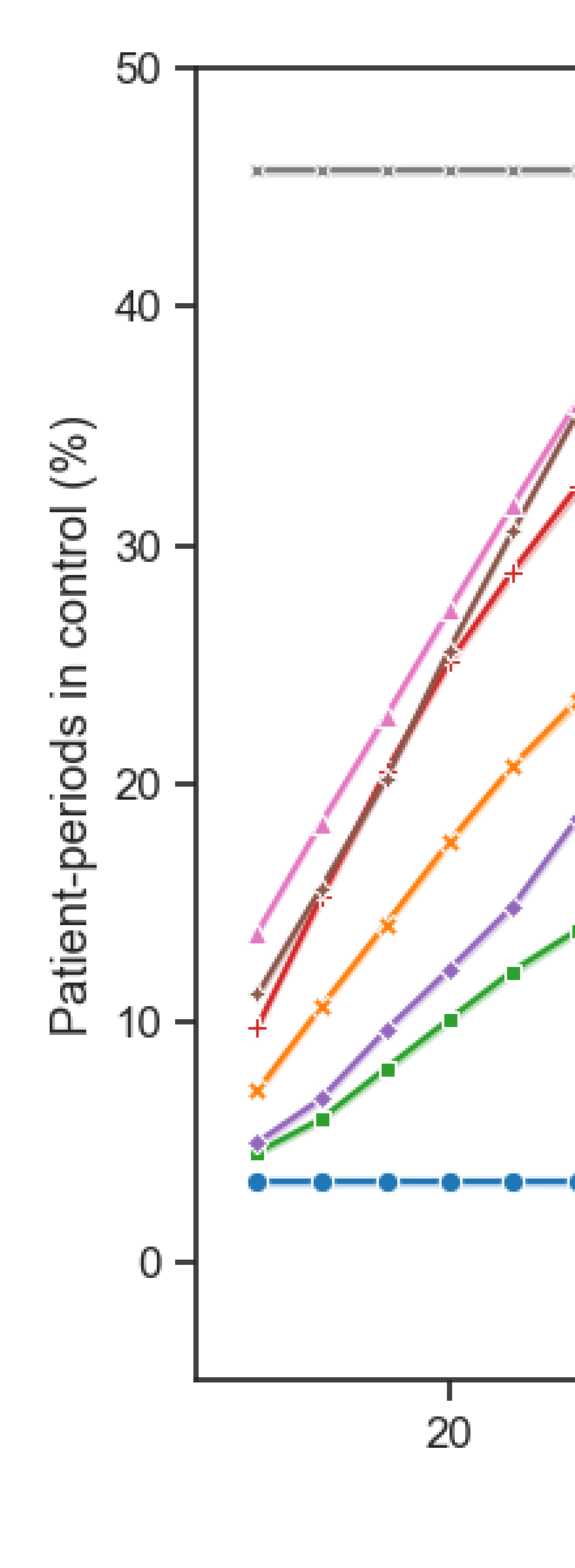
(a) Scenario 1

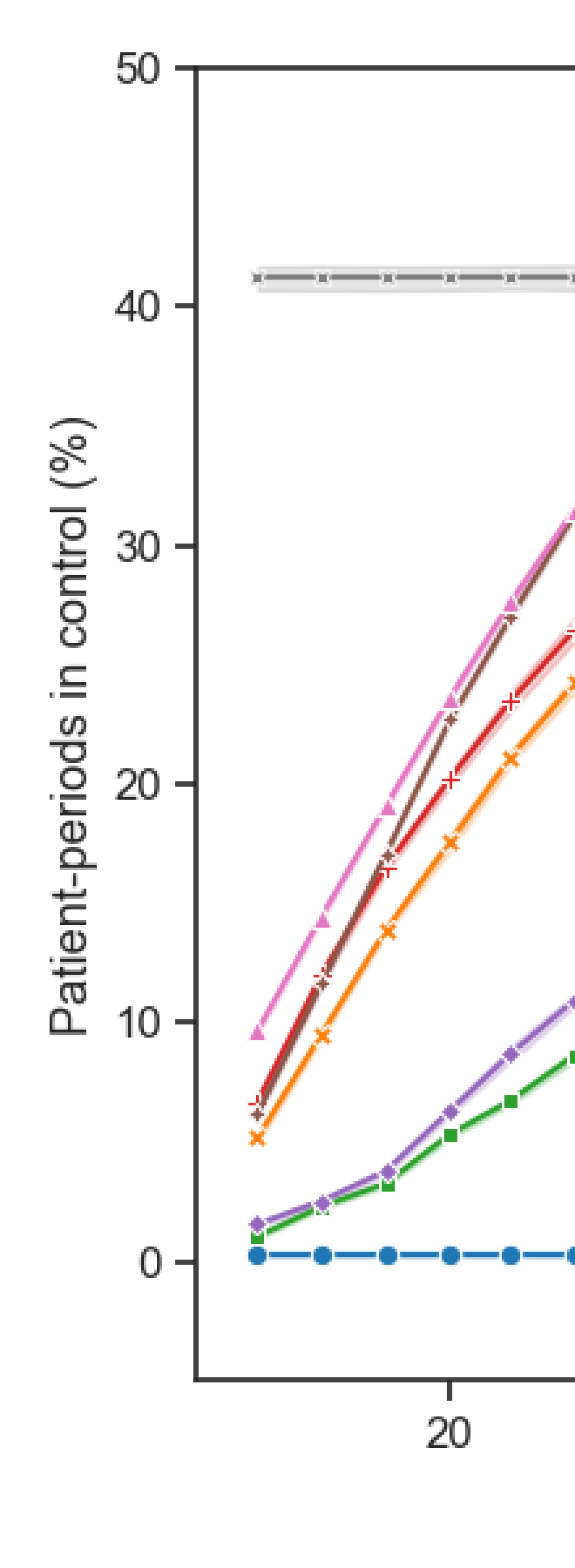
(b) Scenario 2

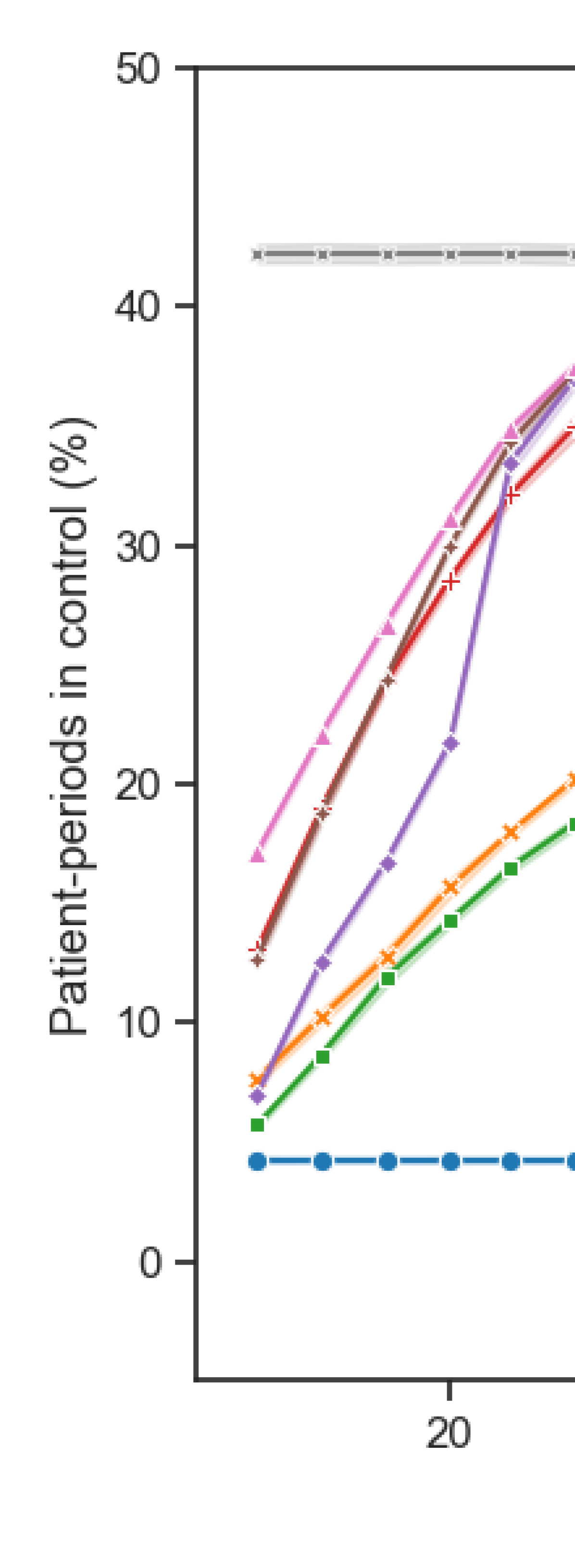
(c) Scenario 3

 

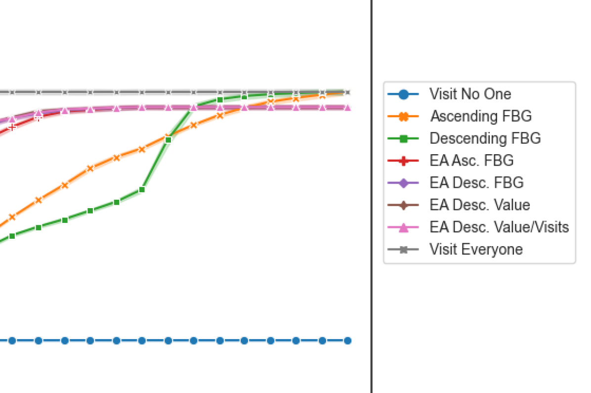
Figure 8: Glycemic control for different scenarios at various capacity levels with shaded 95% confidence intervals.

6.4.2 Visit types and patient enrollment.

Figure 9 shows the proportion of CHW visits that were screening visits for different scenarios throughout the planning horizon. We chose a capacity level of 20% for illustrative purposes. As expected, we observe that screening visits are highest at the start of the horizon for each scenario and model implementation. For the best performing (in terms of PPC) EA implementations (i.e., Desc. Value-to-go/Visits and Desc. Value-to-go), we observe that the proportion of screening visits decreases to (nearly) zero after the first five periods. In contrast, the proportion of screening visits for the benchmark heuristics (i.e., Desc. FBG and Asc. FBG) does not decrease as quickly, and in some cases remains high throughout the planning horizon. There are two primary reasons for this. First, the benchmark heuristics (continuously) screen individuals who do not enroll in the program, effectively wasting visit resources. Second, the benchmark heuristics often screen individuals who enroll, but then drop out due to adverse factors of enrollment because they are either visited too frequently or not enough.

Figure 10 displays the proportion of enrolled patients for different scenarios throughout the planning horizon at 20% capacity. In line with the screening patterns observed in Figure 9, enrollment increases rapidly during the first 5 periods. We observe that the best performing implementation (EA Desc. Value/Visits) maintains roughly 30% enrollment across all scenarios, suggesting that there exists an enrollment “sweet spot”. Intuitively, this makes sense for two reasons. First, if we enroll too many patients, we may not have the capacity to conduct management visits causing patients to drop out (and then need to be re-screened). Second, if we do not enroll enough patients, we may not make a large enough impact and we may have excess capacity and over-visit patients, causing them to drop out. Again, we see that the EA implementation with the strongest value function approximation can determine the best patient pool size and its composition (the patients who the CHW intervention ought to enroll) to maximize PPC.

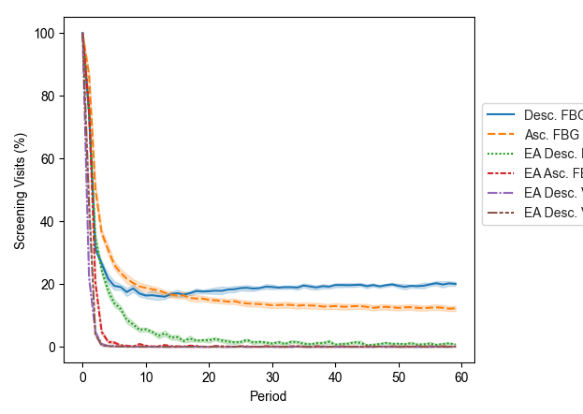
(a) Scenario 1

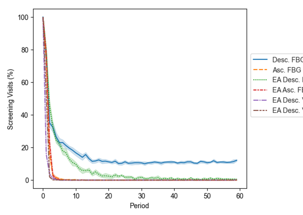
(b) Scenario 2

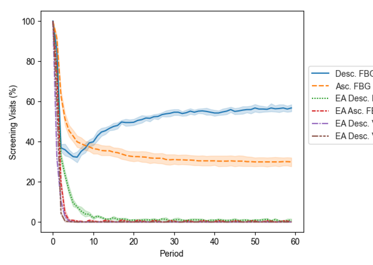
(c) Scenario 3

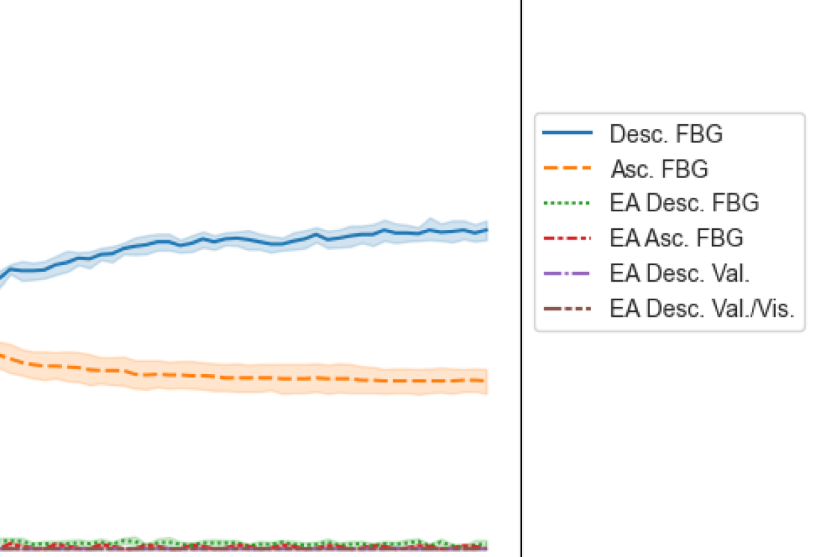
Figure 9: Line graphs for different scenarios showing the proportion of CHW visits that were screening visits at 20% capacity with shaded 95% confidence intervals.

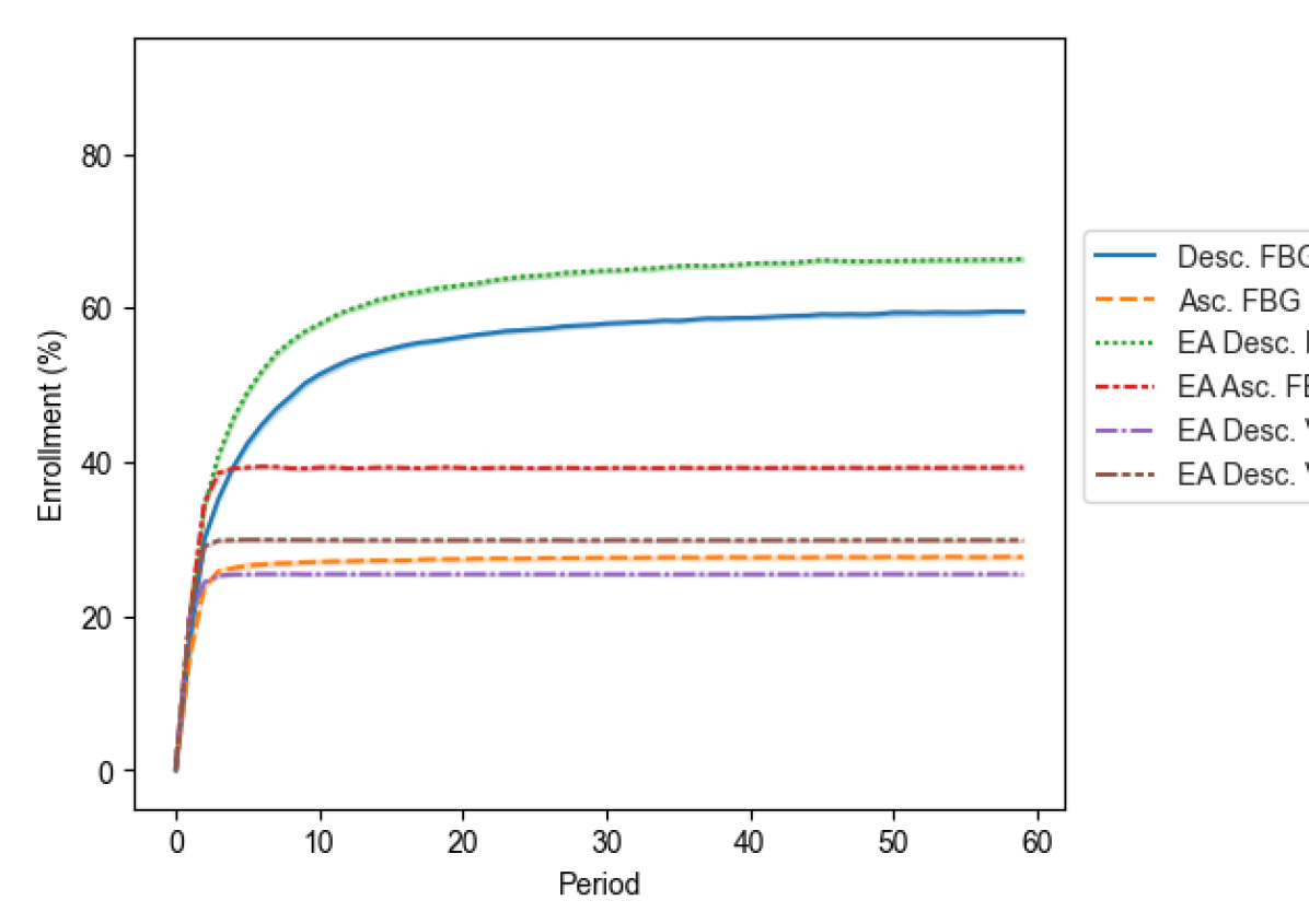
(a) Scenario 1

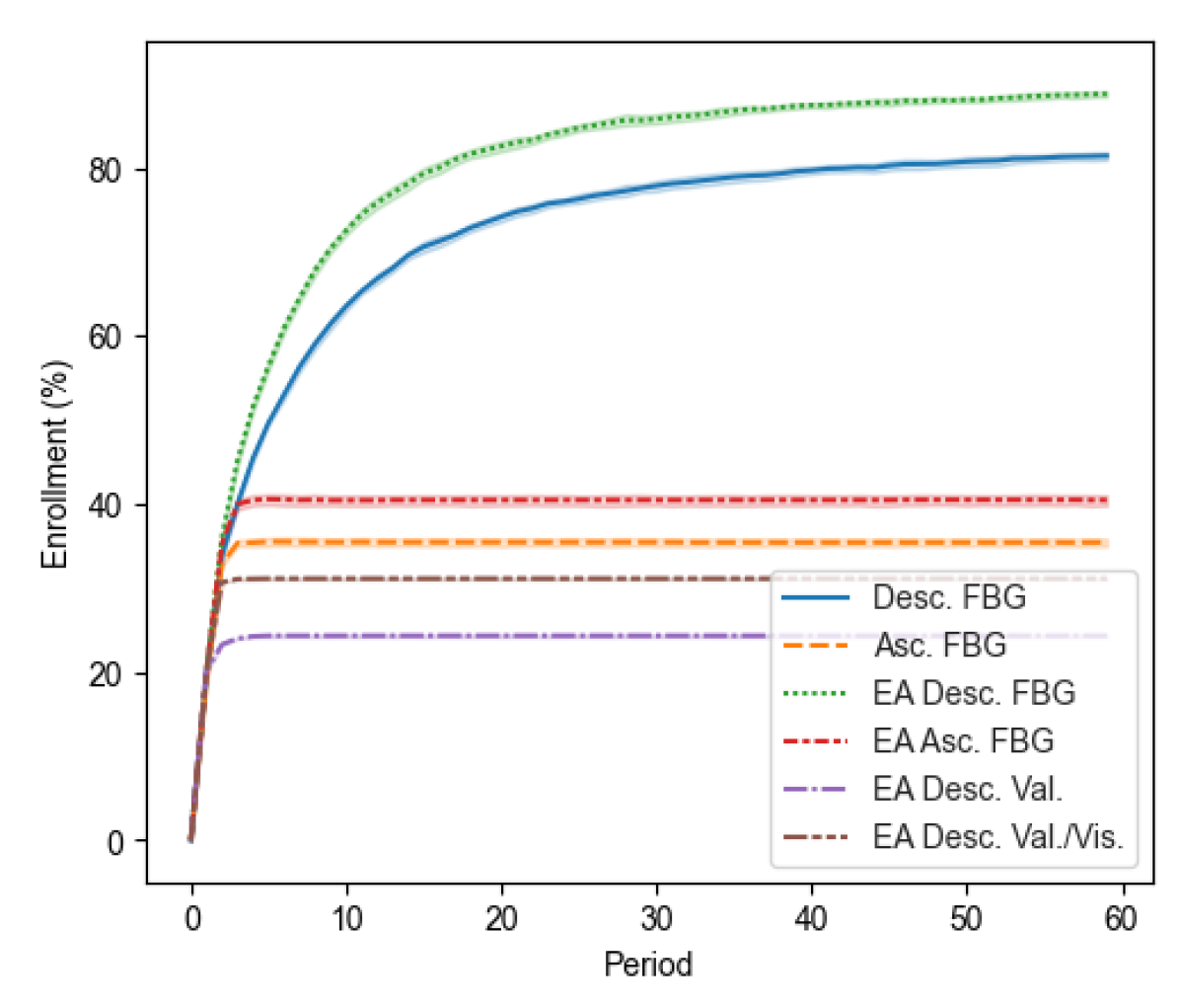
(b) Scenario 2

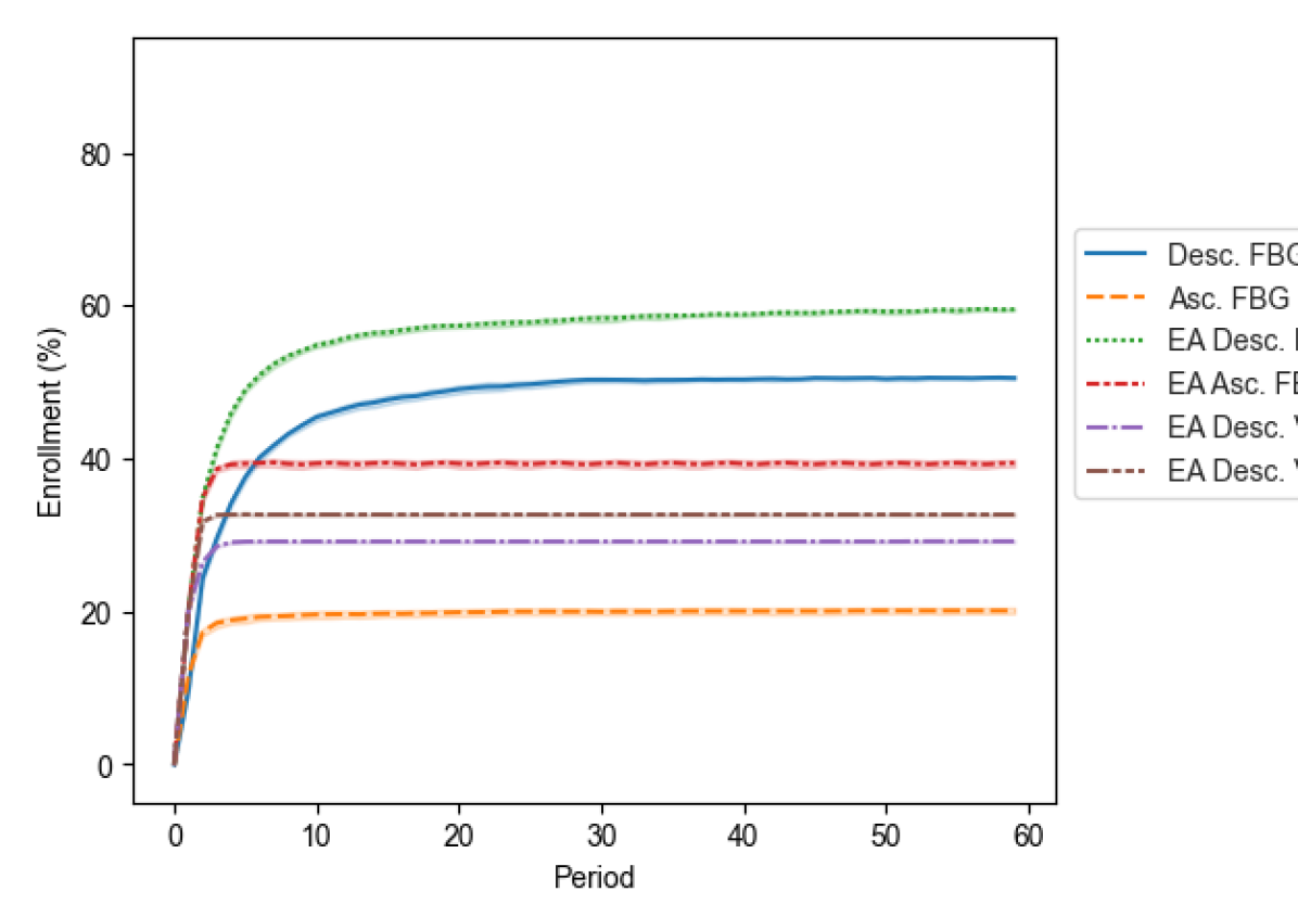
(c) Scenario 3

Figure 10: Line graphs for different scenarios showing the proportion of patients enrolled in treatment at 20% capacity with shaded 95% confidence intervals.

6.4.3 FBG distribution.

Figure 11 displays violin plots showing the distribution of log-FBG values for different scenarios at the end of the planning horizon. These figures allow us to analyze not only the performance in terms of glycemic control, but also how they prioritize patients. For example, Figure 11(b) shows a bimodal shape for the EA Descending Value-to-go/Visits implementation, suggesting that a subset of patients is prioritized while other patients have their disease progress. These results highlight that in order to maximize PPC, we need to focus our resources on the subset of patients that benefit most from the intervention and effectively ignore the patients who do not benefit (or whose FBG cannot be controlled). Intuitively, this makes sense because we want to be as efficient as possible with our limited resources and those who do not benefit from the program will need to be cared for using other more effective (for them) interventions. Similarly to what we observed in Section 6.4.2, where the EA implementation with the best PPC performance maintained lower enrollment than some of the alternatives (e.g., EA Desc. FBG), there is an efficiency-equity tradeoff to be considered by the provider in terms of managing the FBG distribution in the targeted community.

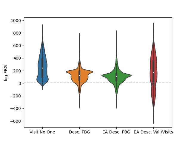
(a) Scenario 1

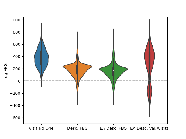
(b) Scenario 2

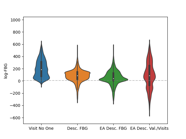
(c) Scenario 3

Figure 11: Violin plots showing the distribution of log-FBG values at the end of the planning horizon for different scenarios based on the implementation of four methods: Visit No One, Descending FBG with 20% capacity, EA Descending FBG with 20% capacity, and EA Descending Value-to-go/Visits with 20% capacity. The gray dashed line indicates the FBG threshold $\delta$.

6.5 Managerial Implications

Our work has relevant implications not only for NanoHealth’s operations, but also for other CHW interventions for chronic diseases. We highlight the following key managerial implications:

1. Given the competing objectives of equity and efficiency, there is no ‘one-size-fits-all’ solution to plan CHW interventions. Through our computational experiments and analysis, we found that cohort composition, capacity level, and intervention goals all affect the choice of the best CHW visit plan. We presented results where simple benchmark heuristics had a comparable performance to the EA implementations (e.g., NanoHealth’s cohort for capacities lower than 20%; see Figure 3), as well as results where using the best benchmark heuristic would require up to 161.5% greater capacity than using the best EA implementations to achieve the same performance (i.e., achieving 30% PPC in Scenario 3; see Figure 8(c)). In the case of the EA implementation with the best PPC performance (consistent across all scenarios and at most capacity levels), the EA Descending Value-to-go/Visits, efficiency led to a lower percentage of patients enrolled in treatment (see Figure 10) and to some patients being prioritized while others were left out of CHW visit plans (indicated by a lower 25th percentile and higher median than some alternatives; see Figure 11). In this sense, one of our key contributions is the development of a flexible framework for breaking ties among patients of interest that can be tailored by providers to meet their priorities, patient needs, and resource availability.

2. Incorporating patient motivational and health states is key to efficient resource use in CHW interventions, especially with heterogeneous patient cohorts. We observe that the benchmark heuristics spend a significant portion of their CHW capacity on screening new patients rather than providing management visits to patients that are already enrolled in treatment (see Figures 4 and 9). This results in patients frequently being screened and then immediately dropping from the program, effectively wasting visit resources. On the other hand, since EA incorporates personalized behavioral states, it is able to better serve the patient population and target potential patients that are likely to remain in the program for a long time. Moreover, the EA personalizes visit frequency for enrolled patients avoiding visiting patients too often or not often enough, which can both lead to drop outs and poor glycemic control. At the cohort level, this leads the EA implementations to find an enrollment “sweet spot” (as seen in Figure 10) rather than simply growing the size of the program without consideration to presently enrolled patients, leading to large programs where many patients are ignored in favor of screening patients who may not benefit at all from enrollment.

3. Our framework is scalable and can be implemented on mobile tablets already used by CHW programs. Many CHW programs currently have the infrastructure to implement the EA because they use mobile tablets for data collection and communication. Incorporating the EA approaches would also require using tablets for task list implementation. The EA relies on data typically collected by CHW programs during pilot phases or normal day-to-day operations. Moreover, our technical methods enable providers to identify patient types and to determine how to best personalize their intervention as opposed to providing a one size fits all treatment, all while maintaining a solution method that is computationally tractable.

7 Conclusion

In this paper, we developed a modelling framework to optimize a resource-constrained CHW intervention for diabetes care in urban areas in LMICs. Our framework explicitly models the tradeoff between screening new patients and providing management visits to individuals who are already enrolled in treatment. We account for patients’ motivational states, which affect their decisions to enroll or drop out of treatment and, therefore, the effectiveness of the intervention. We incorporate these decisions by modeling patients as utility-maximizing agents within a bi-level provider problem that we solve using approximate dynamic programming. Our scalable heuristics rely on theoretical results from the single-patient problem that are used to estimate the value function in the multi-patient problem. By performing several simulation experiments, we found that our framework’s performance in terms of patient-periods in control depends on the composition of the patient cohort targeted by the intervention, and can improve upon baseline heuristics by up to 124.5% (in terms of relative performance) using the same CHW capacity. Finally, we applied our approach to generate CHW visit plans for NanoHealth, a social enterprise in India that provided us with the data for our case study. We found that the best EA implementation for NanoHealth’s cohort can achieve the same level of patient-periods in control as the best naive implementation with up to 73.4% less CHW capacity.

Electronic Companion

8 Proofs of Propositions in the Text

Proof 8.1

Proof of Proposition 4.1: Unless otherwise stated, all inequalities and equations hold with probability one. We can write the benefit function for each component of the utility function separately. To write this function for $B^{b}_{i,t}$, we first substitute the dynamic equations for $b_{i,t+1},s_{i,t+1}$ into the utility function components to obtain the following explicit representation in terms of the patient states at time $t$:

$$U_{b}(b_{i,t},z_{i,t}) =-(b_{i,t}+p_{i}-\mu_{i}z_{i,t}-\alpha_{i}y_{i,t}z_{i,t}+\xi_{i,t})$$

$$U_{s}(s_{i,t},\theta_{i,t},z_{i,t}) =-\theta_{i,t}(z_{i,t}(\gamma(s_{i,t}-s_{i,0})+s_{i,0})+\beta_{i}y_{i,t}z_{i,t})$$

Let $B_{i,t}=B^{b}_{i,t}+B^{s}_{i,t}$, where the first component corresponds to the net benefit associated with $b_{i,t}$ and second component corresponds to the net benefit associated with $s_{i,t}$. Then through a similar definition of $B_{i,t}$ by doing the appropriate subtractions we can derive the following forms.

$$B^{b}_{i,t} =\mu_{i}+\alpha_{i}y_{i,t}$$

$$B^{s}_{i,t} =-\theta_{i,t}(\gamma(s_{i,t}-s_{i,0})+s_{i,0})-\theta_{i,t}\beta_{i}y_{i,t}$$

Combining these expressions gives the first result of the proposition.

To obtain the next result note that if $B_{i,t}\geq 0$ this implies that $U_{i}(b_{i,t+1},s_{i,t+1},\theta_{i,t},\xi_{i,t},1)\geq U_{i}(b_{i,t+1},s_{i,t+1},\theta_{i,t},\xi_{i,t},0)$ and thus the utility function is maximized when $z_{i,t}=1$. Likewise, when $B_{i,t}<0$ this means $U_{i}(b_{i,t+1},s_{i,t+1},\theta_{i,t},\xi_{i,t},1)<U_{i}(b_{i,t+1},s_{i,t+1},\theta_{i,t},\xi_{i,t},0)$ and therefore $z_{i,t}=0$. However, $z_{i,t}$ can only be equal to 1 if $y_{i,t}$ or $z_{i,t-1}$ are equal to 1. This gives the second result of the proposition.

Proof 8.2

Proof of Proposition 4.3: We seek to use a MLE approach to estimate all unknown parameters:

$$(\hat{},\hat{\mathbf{s}},\hat{\boldsymbol{\theta}},\hat{\beta},\hat{\alpha},\hat{\mu},\hat{p},\hat{\lambda},\hat{\gamma},\hat{\rho})\in\argmin_{\mathbf{s},\boldsymbol{\theta},\beta,\alpha,\mu,p,\lambda,\gamma,\rho}p(\{\bar{b}_{t}\}_{t\in K}|\mathbf{s},\boldsymbol{\theta},\beta,\alpha,\mu,p,\lambda,\gamma,\rho,\mathbf{z},\mathbf{y},\boldsymbol{\xi})$$ (16)

Using the dynamic equations described in Section 4, we can decompose the likelihood function in (16) as follows:

$$p(\{\tilde{b}_{t}\}_{t\in K}|\mathbf{s},\boldsymbol{\theta},\beta,\alpha,\mu,p,\lambda,\gamma,\rho,\mathbf{z},\mathbf{y},\boldsymbol{\xi})=\prod_{t\in K}p(\tilde{b}_{t}|b_{t})\prod_{t\in T}p(b_{t}|b_{t-1},p,\mu,z_{t},\alpha,y_{t},\xi_{t})\\ p(s_{t}|s_{t-1},s_{0},\beta,y_{t},z_{t},\gamma)p(\theta_{t}|\theta_{t-1},\theta_{0},\lambda,y_{t},z_{t},\rho)p(z_{t}|\mu,\theta_{t},s_{t},s_{0},\alpha,\beta,\gamma,y_{t})p(\xi_{t})$$ (17)

Note that while the product terms related to $\tilde{b}_{t}$ are only taken over time periods $\mathcal{K}\subset\mathcal{T}$, the other terms are taken over all time indices. This is due to the definition of the one step dynamics, and allows us to estimate the values of these parameters during periods for which we do not have direct observations.

Next, we take the log of both sides of the likelihood function in Equation (17) to obtain the log-likelihood:

$$\log p(\{\tilde{b}_{t}\}_{t\in\mathcal{K}}|\mathbf{s},\boldsymbol{\theta},\beta,\alpha,\mu,p,\mathbf{z},\mathbf{y},\boldsymbol{\xi})= \sum_{t\in\mathcal{K}}\log p(\tilde{b}_{t}|b_{t})+\sum_{t\in\mathcal{T}}\log p(b_{t}|b_{t-1},p,\mu,z_{t},\alpha,y_{t},\xi_{t})$$

$$+\log p(s_{t}|s_{t-1},s_{0},\beta,y_{t},z_{t},\gamma)+\log p(\theta_{t}|\theta_{t-1},\theta_{0},\lambda,y_{t},z_{t},\rho)$$

$$+\log p(z_{t}|\mu,\theta_{t},s_{t},s_{0},\alpha,\gamma,\beta,y_{t})+\log p(\xi_{t}).$$

Observe that $p(\tilde{b}_{t}|b_{t})=f_{\epsilon}(\tilde{b}_{t}-b_{t})$ and that $p(\xi_{t})=f_{\xi}(\xi_{t})$ by definition of the disturbance model and note that because the remaining terms correspond to deterministic system dynamics, they are degenerate distributions. Thus, the MLE can be expressed as the following constrained optimization problem:

$$\underset{\mathbf{s},\boldsymbol{\theta},\beta,\alpha,\mu,p,\lambda,\rho,\gamma,\boldsymbol{\xi}}{\mathrm{minimize}}\> \sum_{t\in\mathcal{K}}\log f_{\epsilon}(\tilde{b}_{t}-b_{t})+\sum_{t\in\mathcal{T}}\log f_{\xi}(\xi_{t})$$ (18a)

$$\mathrm{subject\,to}\quad b_{t+1}=b_{t}+p-\mu z_{t}-\alpha y_{t}z_{t}+\xi_{t},\quad\forall t\in\mathcal{T},$$ (18b)

$$s_{t+1}=\gamma z_{t}(s_{t}-s_{0})+z_{t}s_{0}+\beta y_{t}z_{t},\quad\forall t\in\mathcal{T},$$ (18c)

$$\theta_{t+1}=\rho(\theta_{t}-\theta_{0})+\theta_{0}-\lambda y_{t}z_{t},\quad\forall t\in\mathcal{T},$$ (18d)

$$z_{i,t}=(z_{i,t-1}+y_{i,t}-z_{i,t-1}y_{i,t})\mathbbm{1}[B_{i,t}\geq 0]\quad\forall t\in\mathcal{T},$$ (18e)

$$\hat{b}_{t},s_{t},\theta_{t}\geq 0,\quad\forall t\in\mathcal{T},$$ (18f)

$$\beta,\alpha,\mu,p,\lambda,\rho,\gamma\geq 0.$$ (18g)

Constraint (18e) is derived from Proposition 4.1 and the remaining constraints come from the model dynamics. To obtain the final formulation, constraint (18e) is reformulated using disjunctive constraints (Wolsey and Nemhauser 1999).

Proof 8.3

Proof of Lemma 5.1: Since $z_{t-1}\in\{0,1\}$, we simply evaluate $z_{t}$ for $z_{t-1}=0$ and $z_{t-1}=1$:

$$z_{t}(0,y_{t})=y_{t}\cdot\mathbbm{1}(B_{t}(y_{t})\geq 0)\leq\mathbbm{1}(B_{t}(y_{t})\geq 0)=z_{t}(1,y_{t}).\halmos$$

Proof 8.4

Proof of Lemma 5.2: Since $V_{N}$ is only a function of the FBG value, $b_{N}$, and $b_{N}=b_{N-1}+p-\mu z_{N-1}-\alpha y_{N-1}z_{N-1}+\xi_{N-1}$, we have that for any value of $\xi_{N-1}$:

$$V_{N}(b_{N},s_{N},\theta_{N},z_{N-1})=\begin{cases}1,&\text{if }b_{N-1}\leq\delta-p+\mu z_{N-1}(y_{N-1})+\alpha y_{N-1}z_{N-1}(y_{N-1})-\xi_{N-1},\\ 0,&\text{if }b_{N-1}>\delta-p+\mu z_{N-1}(y_{N-1})+\alpha y_{N-1}z_{N-1}(y_{N-1})-\xi_{N-1}.\end{cases}$$

Since $z_{N-1}$ is a binary variable, we evaluate $V_{N}$ for $z_{N-1}=0$ and $z_{N-1}=1$:

$$V_{N}(z_{N-1}=0) =\begin{cases}1,&\text{if }b_{N-1}\leq\delta-p-\xi_{N-1}\\ 0,&\text{if }\delta-p-\xi_{N-1}<b_{N-1}\leq\delta-p+\mu+\alpha y_{N-1}-\xi_{N-1}\\ 0,&\text{if }b_{N-1}>\delta-p+\mu+\alpha y_{N-1}-\xi_{N-1}\end{cases}$$

$$V_{N}(z_{N-1}=1) =\begin{cases}1,&\text{if }b_{N-1}\leq\delta-p-\xi_{N-1}\\ 1,&\text{if }\delta-p-\xi_{N-1}<b_{N-1}\leq\delta-p+\mu+\alpha y_{N-1}-\xi_{N-1}\\ 0,&\text{if }b_{N-1}>\delta-p+\mu+\alpha y_{N-1}-\xi_{N-1}\end{cases}$$

Note that $\delta-p-\xi_{N-1}\leq\delta-p+\mu+\alpha y_{N-1}-\xi_{N-1}$ because $\mu\geq 0$ and $\alpha\geq 0$. Since $V_{N}(z_{N-1}=0)\leq V_{N}(z_{N-1}=1)$ for all values of $b_{N-1}$ and $\xi_{N-1}$, the proof is complete.

Proof 8.5

Proof of Theorem 5.3:

We proceed by induction. For the base case, we need to show that $V_{N-1}$ is nondecreasing in $z_{N-2}$, i.e., $V_{N-1}(z_{N-2}=0)\leq V_{N-1}(z_{N-2}=1)$ for any value of $\xi_{N-2}$, which is equivalent to:

$$\max_{y_{N-1}\in\{0,1\}}\{V_{N}(z_{N-2}=0)\}\leq\max_{y_{N-1}\in\{0,1\}}\{V_{N}(z_{N-2}=1)\}.$$

Observe that $V_{N}$ does not depend directly $z_{N-2}$, but is only affected by it through $z_{N-1}$. Since $V_{N}$ is nondecreasing in $z_{N-1}$ for all values of $\xi_{N-1}$ (Lemma 5.2) and $z_{N-1}$ is nondecreasing in $z_{N-2}$ (Lemma 5.1), it follows that $V_{N}$ is nondecreasing in $z_{N-2}$ since the composition of nondecreasing functions is also nondecreasing for all values of $\xi_{N-1}$. Moreover, since the dependence between $z_{N-1}$ and $z_{N-2}$ is only through $B_{N-1}$ this relationship is functionally independent of $\xi_{N-2}$ meaning the above composition holds for any realization of $\xi_{N-2}$.

Next we can show that $V_{N-1}$ is nondecreasing in $z_{N-2}$. Using Equation (11) we can express $V_{N-1}$ as:

$$V_{N-1}(b_{N-1},s_{N-1},\theta_{N-1},z_{N-2})=\mathbbm{1}[b_{N-1}\leq\delta]+\max_{y_{N-1}\in\{0,1\}}F_{\xi}\big{(}\delta-b_{N-1}-p+\mu z_{N-1}(y_{N-1},z_{N-2})\\ +\alpha y_{N-1}z_{N-1}(y_{N-1},z_{N-2})\big{)},$$ (19)

where $F_{\xi}$ is the c.d.f of $\xi_{t}$. Note that again by Lemma 5.2 and properties of the c.d.f, $V_{N-1}$ is non decreasing in $z_{N-2}$ for any value of $\xi_{N-2}$.

For the inductive hypothesis, we assume that $V_{t+1}$ is nondecreasing in $z_{t}$, that is, $V_{t+1}(z_{t}=0)\leq V_{t+1}(z_{t}=1)$ with probability 1. Finally, we show that $V_{t}$ is nondecreasing in $z_{t-1}$, which follows the same logic as the base case. First, observe that $V_{t}(z_{t-1}=0)\leq V_{t}(z_{t-1}=1)$ is equivalent to

$$\max_{y_{t}\in\{0,1\}}\mathbb{E}_{\xi}\,\{V_{t+1}(z_{t-1}=0)\}\leq\max_{y_{t}\in\{0,1\}}\mathbb{E}_{\xi}\,\{V_{t+1}(z_{t-1}=1)\}.$$

Similar to the base case, $V_{t+1}$ is a composition function of $z_{t-1}$ through $z_{t}$, which is a function of $z_{t-1}$. Since $V_{t+1}$ is nondecreasing in $z_{t}$ (inductive hypothesis), $z_{t}$ is nondecreasing in $z_{t-1}$ (Lemma 5.1), and that expectations over nondecreasing functions preserve their monotonicity, it follows that $\mathbb{E}_{\xi}V_{t+1}$ is nondecreasing in $z_{t-1}$. And, since the maximum of monotonically nondecreasing functions is a monotonically nondecreasing function, we have that $V_{t}$ is nondecreasing in $z_{t-1}$.

Proof 8.6

Proof of Theorem 5.4:

It is sufficient to show that $\mathbb{E}_{\xi}V_{t}(b_{t},s_{t},\theta_{t},z_{t-1})$ is strictly increasing in $y_{t-1}$ for case $(i)$, $\mathbb{E}_{\xi}V_{t}(b_{t},s_{t},\theta_{t},z_{t-1})$ is strictly decreasing in $y_{t-1}$ for case $(ii)$, and $\mathbb{E}_{\xi}V_{t}(b_{t},s_{t},\theta_{t},z_{t-1})$ is constant in $y_{t-1}$ for case $(iii)$. Since we have already shown in Theorem 5.3 that $\mathbb{E}_{\xi}V_{t}$ is nondecreasing in $z_{t-1}$, we only need to show when $z_{t}(z_{t-1},y_{t})=(z_{t-1}+y_{t}-z_{t-1}y_{t})\cdot\mathbbm{1}(B_{t}(y_{t})\geq 0)$ is strictly increasing, strictly decreasing, and constant in $y_{t}$ (which would imply the same relationship between $z_{t-1}$ and $y_{t-1}$). We proceed by enumerating two cases corresponding to $z_{t-1}=0$ and $z_{t-1}=1$.

For the case when $z_{t-1}=1$ (i.e., the patient is enrolled), $z_{t}(1,0)>z_{t}(1,1)$ (i.e., strictly decreasing) if and only if $B_{t}(0)\geq 0$ and $B_{t}(1)<0$, $z_{t}(1,0)<z_{t}(1,1)$ if and only if $B_{t}(0)<0$ and $B_{t}(1)\geq 0$, and $z_{t}(1,0)=z_{t}(1,1)$ if and only if $B_{t}(0)<0$ and $B_{t}(1)<0$ or $B_{t}(0)\geq 0$ and $B_{t}(1)\geq 0$.

For the case when $z_{t-1}=0$ (i.e., the patient is not enrolled), $z_{t}(0,0)$ is never strictly greater than $z_{t}(0,1)$ because $z_{t}(0,0)=0$, $z_{t}(0,0)<z_{t}(0,1)$ if and only if $B_{t}(1)\geq 0$, and $z_{t}(0,0)=z_{t}(0,1)$ if and only if $B_{t}(1)<0$.

Proof 8.7

Proof of Lemma 5.7: Note that the argmax is over the sum of value functions with respect to period $N$ because actions taken in period $N-1$ only impact the FBG (and, therefore, the value function) of the following period, $N$, which is additively decomposable by Equation (14). Note that, in the single period problem, visiting a patient who is not in set $\mathcal{I}_{N-1}$ would result in a patient who would not benefit in the short term from the visit taking resources instead of one who would by Theorem 5.3. Thus we must only consider cases based on the size of set $\mathcal{I}_{N-1}$.

If $|\mathcal{I}_{N-1}|\leq C$, then the proof follows directly from the definition of $\mathcal{I}_{t}$, Theorem 5.3, and Corollary 5.5 because the problem is equivalent to $|\mathcal{I}_{N-1}|$ single patient problems. To prove the claim for the case where $|\mathcal{I}_{N-1}|>C$, we proceed by contradiction. Without loss of generality, assume $\exists j\in\mathcal{S}_{N-1},\ell\notin\mathcal{S}_{N-1}$ such that

$$V_{\ell,N}^{1}-V_{\ell,N}^{0} >V_{j,N}^{1}-V_{j,N}^{0}.$$

Let $\mathcal{S}^{\prime}_{N-1}$ be the set obtained by swapping the elements $j$ and $\ell$, that is, $\mathcal{S}^{\prime}_{N-1}=\mathcal{S}_{N-1}\cup\{\ell\}\setminus\{j\}$. Let us consider the relationship between the value function of visiting patients in set $\mathcal{S}^{\prime}_{N-1}$ instead of $\mathcal{S}_{N-1}$.

$$\sum_{i\notin\mathcal{S}_{N-1}}V_{i,N}^{0}+\sum_{i\in\mathcal{S}_{N-1}}V_{i,N}^{1}$$ (20)

$$=\sum_{i\notin\mathcal{S}_{N-1}\setminus\{\ell\}}V_{i,N}^{0}+\sum_{i\in\mathcal{S}_{N-1}\setminus\{j\}}V_{i,N}^{1}+V_{j,N}^{1}+V_{\ell,N}^{0}$$ (21)

$$<\sum_{i\notin\mathcal{S}_{N-1}\setminus\{\ell\}}V_{i,N}^{0}+\sum_{i\in\mathcal{S}_{N-1}\setminus\{j\}}V_{i,N}^{1}+V_{j,N}^{0}+V_{\ell,N}^{1}$$ (22)

$$=\sum_{i\notin\mathcal{S}^{\prime}_{N-1}}V_{i,N}^{0}+\sum_{i\in\mathcal{S}^{\prime}_{N-1}}V_{i,N}^{1}$$ (23)

However, $\mathcal{S}_{N-1}$ is defined as the set of patients where $y_{i,N-1}=1$ that maximizes the sum of value functions for all patients. Therefore, we have reached a contradiction and conclude the proof.

Proof 8.8

Proof of Proposition 5.8: We will proceed to prove this proposition by induction on $t$. First let us consider the base case, $t=N-1$. Using the dynamic programming equations (13),(14), and Lemma 5.7 we can write the value function at period $N-1$ as:

$$\mathcal{V}_{N-1}(_{N-1},\mathbf{s}_{N-1},\boldsymbol{\theta}_{N-1},\mathbf{z}_{N-2})=\sum_{i\in\mathcal{P}}\mathbbm{1}(b_{i,N-1}\leq\delta)+\sum_{i\in\mathcal{S}_{N-1}}V_{i,N}^{1}+\sum_{i\in\mathcal{P}\setminus\mathcal{S}_{N-1}}V_{i,N}^{0}.$$ (24)

If, for each $i\in\mathcal{P}$, we define $\mathcal{V}_{i,N-1}(b_{i,N-1},s_{i,N-1},\theta_{i,N-1},z_{i,N-2}):=\mathbbm{1}(b_{i,N-1}\leq\delta)+V_{i,N}^{1}\mathbbm{1}(i\in\mathcal{S}_{N-1})+V_{i,N}^{0}(1-\mathbbm{1}(i\in\mathcal{S}_{N-1}))$, then it is clear that from equation (24), $\mathcal{V}_{N-1}(_{N-1},\mathbf{s}_{N-1},\boldsymbol{\theta}_{N-1},\mathbf{z}_{N-2})=\sum_{i\in\mathcal{P}}\mathcal{V}_{i,N-1}(b_{i,N-1},s_{i,N-1},\theta_{i,N-1},z_{i,N-2})$.

Next we proceed with the main induction step. Suppose that for some $t+1\leq N-1$ we have that $\mathcal{V}_{t+1}(_{t+1},\mathbf{s}_{t+1},\boldsymbol{\theta}_{t+1},\mathbf{z}_{t})=\sum_{i\in P}\mathcal{V}_{i,t+1}(b_{i,t+1},s_{i,t+1},\theta_{i,t+1},z_{i,t})$. Using the dynamic programming equations (13) we can thus rewrite the equation for time $t$ as:

$$\mathcal{V}_{t}(_{t},\mathbf{s}_{t},\boldsymbol{\theta}_{t},\mathbf{z}_{t-1})=\sum_{i\in\mathcal{P}}\mathbbm{1}(b_{i,t}\leq\delta)+\max_{\sum_{i\in\mathcal{P}}y_{i,t}\leq C,y_{i,t}\in\mathbb{B}}\sum_{i\in\mathcal{P}}\mathbb{E}_{\boldsymbol{\xi}}\mathcal{V}_{i,t+1}(b_{i,t+1}(y_{i,t}),s_{i,t+1}(y_{i,t}),\theta_{i,t+1}(y_{i,t}),z_{i,t}(y_{i,t}))$$ (25)

Note that, since $y_{i,t}\in\mathbb{B}$, it can only take on values of either 0 or 1 in the solution to the second term of Equation 25. Let $\mathcal{A}_{t}\subset\mathcal{P}$ be defined as $\mathcal{A}_{t}:=\{i\in\mathcal{P}:y^{*}_{i,t}=1\}$ where $\mathbf{y}^{*}\in\argmax_{\sum_{i\in\mathcal{P}}y_{i,t}\leq C,y_{i,t}\in\mathbb{B}}\sum_{i\in\mathcal{P}}\mathbb{E}_{\boldsymbol{\xi}}\mathcal{V}_{i,t+1}(b_{i,t+1}(y_{i,t}),s_{i,t+1}(y_{i,t}),\theta_{i,t+1}(y_{i,t}),z_{i,t}(y_{i,t}))$. If $\mathcal{A}_{t}=\emptyset$ or $\mathcal{A}_{t}=\mathcal{P}$ then the result of the proposition trivially follows by the induction hypothesis. If $\mathcal{A}_{t}$ is a proper non-empty subset of $\mathcal{P}$ then we can form a partition similar to the base case as follows:

$$\mathcal{V}_{t}(_{t},\mathbf{s}_{t},\boldsymbol{\theta}_{t},\mathbf{z}_{t-1})=\sum_{i\in\mathcal{P}}\mathbbm{1}(b_{i,t}\leq\delta)+\sum_{i\in\mathcal{A}_{t}}V_{i,t+1}^{1}+\sum_{i\in\mathcal{P}\setminus\mathcal{A}_{t}}V_{i,t+1}^{0}$$ (26)

Defining $\mathcal{V}_{i,t}(b_{i,t},s_{i,t},\theta_{i,t},z_{i,t-1}):=\mathbbm{1}(b_{i,t}\leq\delta)+V_{i,t+1}^{1}\mathbbm{1}(i\in\mathcal{A}_{t})+V_{i,t+1}^{0}(1-\mathbbm{1}(i\in\mathcal{A}_{t}))$, and rewriting (26) thus completes the proof.

Proof 8.9

Proof of Proposition 5.9: Again we will proceed to prove this proposition by induction on $t$. First we consider the base case of $t=N-1$. Recall that the component functions at $t=N-1$ are defined as $\mathcal{V}_{i,N-1}(b_{i,N-1},s_{i,N-1},\theta_{i,N-1},z_{i,N-2}):=\mathbbm{1}(b_{i,N-1}\leq\delta)+V_{i,N}^{1}\mathbbm{1}(i\in\mathcal{S}_{N-1})+V_{i,N}^{0}(1-\mathbbm{1}(i\in\mathcal{S}_{N-1}))$. The first term in this definition doesn’t depend on $z_{i,N-2}$ so we only need to focus on the last two terms. Since these last terms are equivalent to the terms of a one-step single patient problem, they are clearly nondecreasing in $z_{i,N-2}$ by Lemma 5.1 and Lemma 5.2.

For the main induction step, consider the induction hypothesis that for some $t+1\leq N-1$ for all patients $i\in\mathcal{P}$, $\mathcal{V}_{i,t+1}(b_{i,t+1},s_{i,t+1},\theta_{i,t+1},z_{i,t})$ is nondecreasing in $z_{i,t}$. Now consider $\mathcal{V}_{i,t}(b_{i,t},s_{i,t},\theta_{i,t},z_{i,t-1})=\mathbbm{1}(b_{i,t}\leq\delta)+V_{i,t+1}^{1}\mathbbm{1}(i\in\mathcal{A}_{t})+V_{i,t+1}^{0}(1-\mathbbm{1}(i\in\mathcal{A}_{t}))$, where $\mathcal{A}_{t}$ are defined similarly as in Proposition 5.8. Then by direct application of Lemma 5.1 and using the induction hypothesis, we obtain the desired result.

Proof 8.10

Proof of Theorem 5.10: First note that if $|\mathcal{P}|\leq C$ then the problem is unconstrained and the result follows trivially from Corollary 5.5. So for the remainder of the proof we will consider the constrained case when $|\mathcal{P}|>C$.

Now let us consider the case where, at some time $t$, $|\mathcal{I}_{t}|\leq C$. Suppose for a contradiction that in this case a visit is allocated to $j\notin\mathcal{I}_{t}$. To show that $\mathcal{I}_{t}=\mathcal{S}_{t}$ is indeed the optimal set of indices to visit it will suffice to show that for $j$ we have $V_{j,t}^{1}\leq V_{j,t}^{0}$ since that would mean we cannot improve the value function by visiting $j$. By definition of $\mathcal{I}_{t}$, since $j\notin\mathcal{I}_{t}$, one of the following two conditions must hold: either (a) $B_{j,t}(y_{j,t}=1)<0$ or (b) $B_{j,t}(y_{j,t}=1)\geq 0$, $z_{j,t-1}=1$ and $B_{j,t}(y_{j,t}=1)\leq B_{j,t}(y_{j,t}=0)$. First let us consider case (a). Note that, in this case, by Proposition 5.9 and Lemma 5.1, it is clear that $V_{j,t}^{1}\leq V_{j,t}^{0}$, with equality holding when $B_{j,t}(y_{j,t}=0)<0$. Now consider case (b). By Proposition 5.9 and Lemma 5.1, it directly follows that $V_{j,t}^{1}=V_{j,t}^{0}$, so clearly the objective would not be improved by visiting $j$, thus yielding the desired result. This establishes that at any point in time visiting patients from set $\mathcal{I}_{t}$ provides an optimal policy.

Next we consider the case where $|\mathcal{I}_{t}|>C$, meaning $\mathcal{S}_{t}$ is a strict subset of $\mathcal{I}_{t}$. In this case, the result of the theorem follows by a similar argument to that of the proof of Lemma 5.7.

9 Patient parameter estimation

To solve the MLE problem in Proposition 4.3, we performed grid search on four parameters ($s_{0}$, $\beta$, $\gamma$ and $\rho$), where we searched over $S=\{0,1,2,3\}$ for $s_{0}$, $B=\{0,1,2,3\}$ for $\beta$, $G=\{0.2,0.5,0.8,0.9,0.99\}$ for $\gamma$, and $R=\{0.2,0.5,0.8,0.9,0.99\}$ for $\rho$. We define the following variables for the grid search procedure. Let $x^{*}$ denote the best optimal solution found through grid search and let $w^{*}$ denote corresponding optimal value. We let $\bar{x}$ be a variable that stores the current best optimal solution, let $\bar{w}$ be a variable that stores the current best optimal value, let $w^{\textnormal{UB}}$ denote the upper bound on $w^{*}$ to initialize the algorithm, and let $q$ represent the optimal value to a particular grid search instance obtained by solving the parameter estimation problem stated in Proposition 4.3 (denoted below as optProb).

Data: $(\mathbf{y},\mathbf{z},\bar{},S,B,G,R)$

Result: $w^{*}$, $x^{*}$ = ($\hat{}^{*}$, $\mathbf{s}^{*}$, $\boldsymbol{\theta}^{*}$, $p^{*}$, $\mu^{*}$, $\alpha^{*}$, $\theta_{0}^{*}$, $\lambda^{*}$, $s_{0}^{*}$, $\beta^{*}$, $\gamma^{*}$, $\rho^{*}$)

begin

       $\bar{w}=w^{\textnormal{UB}}$

      $\bar{x}=\emptyset$

      searchGrid = list($S\times B\times G\times R$)

      for $i\in|S\times B\times G\times R|$ do

             $s_{0}^{i}$, $\beta^{i}$, $\gamma^{i}$, $\rho^{i}$ = searchGrid[$i$]

            ($w$, $\hat{}$, $\mathbf{s}$, $\boldsymbol{\theta}$, $p$, $\mu$, $\alpha$, $\theta_{0}$, $\lambda$) = optProb($\mathbf{y}$, $\mathbf{z}$, $\bar{}$, $s_{0}^{i}$, $\beta^{i}$, $\gamma^{i}$, $\rho^{i}$)

            if $w<\bar{w}$ then

                   $\bar{w}=w$

                  $\bar{x}$ = ($\hat{}$, $\mathbf{s}$, $\boldsymbol{\theta}$, $p$, $\mu$, $\alpha$, $\theta_{0}$, $\lambda$, $s_{0}^{i}$, $\beta^{i}$, $\gamma^{i}$, $\rho^{i}$)

            

      

      $w^{*}=\bar{w}$

      $x^{*}=\bar{x}$

Algorithm 1 Coarse grid search for parameter estimation.

10 NanoHealth patient parameter estimation results

We solved the problem stated in Proposition 4.3 using patient visit history data from NanoHealth (described in Section 6.1.1). Then, we used $k$-means clustering to partition NanoHealth’s patient cohort into distinct clusters based on seven features: FBG progression ($p$), effect of enrollment ($\mu$), effect of a visit ($\alpha$), baseline perception of adverse factors ($\theta_{0}$), decrease in perception of adverse factors per visit ($\lambda$), baseline in adverse factors state ($s_{0}$), and increase in adverse factors per visit ($\beta$). We used an elbow plot to identify the ideal number of clusters: four. Table 1 displays the proportion of patients in each cluster and the mean patient parameter values for each cluster (i.e., the centroid).

Patient parameter	Cluster
	0	1	2	3
Disease progression ($p$)	0.091	6.994	0.039	6.990
Enrollment effect ($\mu$)	0.006	6.899	0.009	0.011
Visit effect ($\alpha$)	0.109	0.125	0.050	6.997
Baseline perception of adverse factors ($\theta_{0}$)	0.001	0	0.002	0
Reduction in perception of adverse factors ($\lambda$)	0	0	0.001	0
Baseline adverse factors ($s_{0}$)	0.072	0	0.060	0
Increase in adverse factors ($\beta$)	0	0.011	1.040	0
% of patients	47.9%	23.8%	26.5%	1.9%
No. of patients ($N=378$)	181	90	100	7

Table 1: Cluster centroids and the percentage of patients in each cluster for NanoHealth’s cohort

11 Enrollment algorithm details

Algorithm 2 provides a detailed description of the enrollment algorithm.

Data: $(P,C,N,f)$: Set of patients with known initial states and parameters, capacity, length of planning horizon, heuristic sorting function.

Result: $\hat{S}$: Visit schedule specifying which patients should be visited in each period.

begin

       for $t\in\{1,\dots,N\}$ do

             for $i\in\{1,\dots,|\mathcal{P}|\}$ do

                   if $i$ meets conditions in Corollary 5.5 then

                         $\mathcal{I}_{t}\longleftarrow\mathcal{I}_{t}\cup\{i\}$

                  

            if $|\mathcal{I}_{t}|\leq C$ then

                   $\hat{\mathcal{S}}_{t}\longleftarrow\mathcal{I}_{t}$

            else

                   $\bar{\mathcal{I}}_{t}\longleftarrow f(\mathcal{I}_{t})$ $\triangleright$ Sort set $\mathcal{I}_{t}$ based on chosen heuristic to obtain the sequence $\bar{\mathcal{I}}_{t}$

                  $\hat{\mathcal{S}}_{t}\longleftarrow\{(a_{n})_{n=1}^{C}|a_{n}\in\bar{\mathcal{I}}_{t}\}$ $\triangleright$ Select first $C$ patients from $\bar{\mathcal{I}}_{t}$ to be visited in period $t$

            for $i\in\{1,\dots,|\mathcal{P}|\}$ do

                   if $i\in\hat{\mathcal{S}}_{t}$ then

                         $y_{i,t}=1$

                  else

                         $y_{i,t}=0$

                  

                  $\>\>\>z_{i,t}=(z_{i,t-1}+y_{i,t}-z_{i,t-1}y_{i,t})\mathbbm{1}[B_{i,t}\geq 0]$

                   $b_{i,t+1}=b_{i,t}+p_{i}-\mu_{i}z_{i,t}-\alpha_{i}y_{i,t}z_{i,t}$

                   $s_{i,t+1}=z_{i,t}(\gamma(s_{i,t}-s_{i,0})+s_{i,0})+\beta_{i}y_{i,t}z_{i,t}$

                   $\theta_{i,t+1}=\rho(\theta_{i,t}-\theta_{i,0})+\theta_{i,0}-\lambda_{i}y_{i,t}z_{i,t}$

            

      

Algorithm 2 Enrollment algorithm

12 Numerical experiments

Table 2 provides summary statistics for the NanoHealth cohort and Table 4 provides summary statistics for five patient groups and corresponding scenarios. Table 3 presents the missingness for each feature.

Characteristic
Number of patients		378
Age in years, mean (sd)		53.3 (11.0)
Female, n (%)		219 (59.2)
Body mass index (kg/m2), mean (sd)		27.6 (5.9)
Waist circumference (inches), mean (sd)		37.1 (4.3)
Heart rate (beats per minute), mean (sd)		83.9 (12.3)
Diastolic blood Pressure (mmHg), mean (sd)		90.2 (11.9)
Systolic blood Pressure (mmHg), mean (sd)		138.2 (21.6)
Tobacco smoker, n (%)		29 (7.8)
Initial FBG (mg/dL), mean (sd)		175.1 (71.9)
Final FBG (mg/dL), mean (sd)		156.8 (61.6)
Number of management visits, mean (sd)		13.1 (7.6)
Visits per month, mean (sd)		0.6 (0.4)

Table 2: Summary statistics from NanoHealth’s patient cohort. See Table  3 for the number of missing observations for each characteristic.

Characteristic		Number of missing observations
Age in years		8 (2.1%)
Female		8 (2.1%)
Body mass index		133 (35.2%)
Waist circumference		147 (38.9%)
Heart rate		119 (31.5%)
Diastolic blood Pressure		8 (2.1%)
Systolic blood Pressure		18 (4.8%)
Tobacco smoker		8 (2.1%)
Initial FBG		8 (2.1%)
Final FBG		0
Number of management visits		0
Visits per month		0

Table 3: Missingness for NanoHealth’s patient cohort.

Patient	Group
parameter	A	B	C	D	E
$p$	0.05	5	5	7.5	0.05
$\mu$	0.025	4	2	4	0.025
$\alpha$	0.1	2	4	2	0.35
$\theta_{0}$	0.7	0.7	0.7	0.7	2
$\lambda$	0.5	0.5	0.5	0.5	1.5
$s_{0}$	1	0.2	0.2	0.2	0.2
$\beta$	0.3	1.5	1.5	1.5	1.5
Simulation cohort composition
Scenario 1	20%	20%	20%	20%	20%
Scenario 2	0%	50%	0%	50%	0%
Scenario 3	0%	50%	0%	0%	50%

Table 4: The table displays the mean value for each parameter for each group and the percentage of patients in each group. The bottom panel displays the percentage of patients from each group in the corresponding artificial cohort for each scenario.

References

- Abdoli et al. (2018) Abdoli S, Doosti Irani M, Hardy LR, Funnell M (2018) A discussion paper on stigmatizing features of diabetes. Nursing open 5(2):113–119.
- Acimovic and Graves (2015) Acimovic J, Graves SC (2015) Making better fulfillment decisions on the fly in an online retail environment. Manufacturing & Service Operations Management 17(1):34–51.
- Alaofè et al. (2017) Alaofè H, Asaolu I, Ehiri J, Moretz H, Asuzu C, Balogun M, Abosede O, Ehiri J (2017) Community health workers in diabetes prevention and management in developing countries. Annals of global health 83(3-4):661–675.
- Aswani et al. (2019) Aswani A, Kaminsky P, Mintz Y, Flowers E, Fukuoka Y (2019) Behavioral modeling in weight loss interventions. European Journal of Operational Research 272(3):1058–1072.
- Ayer et al. (2019) Ayer T, Zhang C, Bonifonte A, Spaulding AC, Chhatwal J (2019) Prioritizing hepatitis C treatment in US prisons. Operations Research 67(3):853–873.
- Ayvaci et al. (2012) Ayvaci MU, Alagoz O, Burnside ES (2012) The effect of budgetary restrictions on breast cancer diagnostic decisions. Manufacturing & Service Operations Management 14(4):600–617.
- Banker et al. (2021) Banker KK, Liew D, Ademi Z, Owen AJ, Afroz A, Magliano DJ, Zomer E (2021) The impact of diabetes on productivity in india. Diabetes care 44(12):2714–2722.
- Bastani and Bayati (2020) Bastani H, Bayati M (2020) Online decision making with high-dimensional covariates. Operations Research 68(1):276–294.
- Bhaskaran et al. (2021) Bhaskaran S, Erzurumlu SS, Ramachandran K (2021) Sequential product development and introduction by cash-constrained start-ups. Manufacturing & Service Operations Management 23(6):1505–1523.
- Billingsley (1961) Billingsley P (1961) The lindeberg-levy theorem for martingales. Proceedings of the American Mathematical Society 12(5):788–792.
- Bonora and Tuomilehto (2011) Bonora E, Tuomilehto J (2011) The pros and cons of diagnosing diabetes with a1c. Diabetes care 34(Supplement_2):S184–S190.
- Boutilier and Chan (2020) Boutilier JJ, Chan TC (2020) Ambulance emergency response optimization in developing countries. Operations Research 68(5):1315–1334.
- Boutilier et al. (2021a) Boutilier JJ, Chan TC, Ranjan M, Deo S (2021a) Risk stratification for early detection of diabetes and hypertension in resource-limited settings: machine learning analysis. Journal of Medical Internet Research 23(1):e20123.
- Boutilier et al. (2021b) Boutilier JJ, Jonasson JO, Yoeli E (2021b) Improving tuberculosis treatment adherence support: The case for targeted behavioral interventions. Manufacturing & Service Operations Management .
- Brunskill and Lesh (2010) Brunskill E, Lesh N (2010) Routing for rural health: optimizing community health worker visit schedules. 2010 AAAI Spring Symposium Series.
- Busza et al. (2018) Busza J, Simms V, Dziva Chikwari C, Dauya E, Bandason T, Makamba M, McHugh G, Ferrand RA (2018) “It is not possible to go inside and have a discussion”: how fear of stigma affects delivery of community-based support for children’s HIV care. AIDS care 30(7):903–909.
- Cawley (2004) Cawley J (2004) An economic framework for understanding physical activity and eating behaviors. American Journal of Preventive Medicine 27(3):117–125.
- Cherkesly et al. (2019) Cherkesly M, Rancourt MÈ, Smilowitz KR (2019) Community healthcare network in underserved areas: design, mathematical models, and analysis. Production and Operations Management 28(7):1716–1734.
- Choudhury (2022) Choudhury S (2022) Average income of indian family is rs 23,000 per month: Survey. https://www.india.com/business/average-income-of-indian-family-is-rs-23000-per-month-survey-5725299/.
- Deo et al. (2013) Deo S, Iravani S, Jiang T, Smilowitz K, Samuelson S (2013) Improving health outcomes through better capacity allocation in a community-based chronic care model. Operations Research 61(6):1277–1294.
- Deo et al. (2022) Deo S, Mehta S, Corbett CJ (2022) Optimal Scale-Up of HIV Treatment Programs in Resource-Limited Settings Under Supply Uncertainty. Production and Operations Management 31(3):883–905.
- Deo et al. (2015) Deo S, Rajaram K, Rath S, Karmarkar US, Goetz MB (2015) Planning for HIV screening, testing, and care at the Veterans Health Administration. Operations research 63(2):287–304.
- Deo and Singh (2018) Deo S, Singh P (2018) Evaluation of a novel community-based chronic disease management solution (Mohali, India: Max Institute for Healthcare Management, Indian School of Business).
- Deo and Singh (2021) Deo S, Singh P (2021) Community health worker-led, technology-enabled private sector intervention for diabetes and hypertension management among urban poor: a retrospective cohort study from large indian metropolitan city. BMJ open 11(8):e045246.
- Derendorf and Meibohm (1999) Derendorf H, Meibohm B (1999) Modeling of pharmacokinetic/pharmacodynamic (pk/pd) relationships: concepts and perspectives. Pharmaceutical Research 16(2):176–185.
- Dieleman et al. (2017) Dieleman J, Campbell M, Chapin A, Eldrenkamp E, Fan VY, Haakenstad A, Kates J, Liu Y, Matyasz T, Micah A, et al. (2017) Evolution and patterns of global health financing 1995–2014: development assistance for health, and government, prepaid private, and out-of-pocket health spending in 184 countries. The Lancet 389(10083):1981–2004.
- Directorate of Economics and Statistics (2015) Directorate of Economics and Statistics (2015) Statistical Year Book. https://www.telangana.gov.in/PDFDocuments/Statistical%20Year%20Book%202015.pdf.
- Emerging Risk Factors Collaboration (2010) Emerging Risk Factors Collaboration (2010) Diabetes mellitus, fasting blood glucose concentration, and risk of vascular disease: a collaborative meta-analysis of 102 prospective studies. The Lancet 375(9733):2215–2222.
- Farias and Madan (2011) Farias VF, Madan R (2011) The irrevocable multiarmed bandit problem. Operations Research 59(2):383–399.
- Fisher et al. (2014) Fisher L, Hessler D, Masharani U, Strycker L (2014) Impact of baseline patient characteristics on interventions to reduce diabetes distress: the role of personal conscientiousness and diabetes self-efficacy. Diabetic Medicine 31(6):739–746.
- Flood et al. (2021) Flood D, Seiglie JA, Dunn M, Tschida S, Theilmann M, Marcus ME, Brian G, Norov B, Mayige MT, Gurung MS, et al. (2021) The state of diabetes treatment coverage in 55 low-income and middle-income countries: a cross-sectional study of nationally representative, individual-level data in 680 102 adults. The Lancet Healthy Longevity 2(6):e340–e351.
- Glazebrook et al. (2006) Glazebrook KD, Ruiz-Hernandez D, Kirkbride C (2006) Some indexable families of restless bandit problems. Advances in Applied Probability 38(3):643–672.
- Gucciardi et al. (2008) Gucciardi E, DeMelo M, Offenheim A, Stewart DE (2008) Factors contributing to attrition behavior in diabetes self-management programs: a mixed method approach. BMC health services research 8(1):1–11.
- Gyawali et al. (2021) Gyawali B, Sharma R, Mishra SR, Neupane D, Vaidya A, Sandbæk A, Kallestrup P (2021) Effectiveness of a female community health volunteer–delivered intervention in reducing blood glucose among adults with type 2 diabetes: An open-label, cluster randomized clinical trial. JAMA network open 4(2):e2035799–e2035799.
- Hajjar and Alagoz (2022) Hajjar A, Alagoz O (2022) Personalized disease screening decisions considering a chronic condition. Management Science .
- Heckman et al. (2015) Heckman BW, Mathew AR, Carpenter MJ (2015) Treatment burden and treatment fatigue as barriers to health. Current opinion in psychology 5:31–36.
- Hoyer et al. (2018) Hoyer A, Rathmann W, Kuss O (2018) Utility of hba1c and fasting plasma glucose for screening of type 2 diabetes: a meta-analysis of full roc curves. Diabetic Medicine 35(3):317–322.
- International Diabetes Federation (2021) International Diabetes Federation (2021) IDF Diabetes Atlas (International Diabetes Federation), 10th edition.
- Jeet et al. (2017) Jeet G, Thakur J, Prinja S, Singh M (2017) Community health workers for non-communicable diseases prevention and control in developing countries: evidence and implications. PloS one 12(7):e0180640.
- Jónasson et al. (2017) Jónasson JO, Deo S, Gallien J (2017) Improving hiv early infant diagnosis supply chains in sub-saharan africa: Models and application to mozambique. Operations Research 65(6):1479–1493.
- Kazibwe et al. (2021) Kazibwe J, Tran PB, Annerstedt KS (2021) The household financial burden of non-communicable diseases in low-and middle-income countries: a systematic review. Health research policy and systems 19(1):96.
- Keyvanshokooh et al. (2021) Keyvanshokooh E, Shi C, Van Oyen MP (2021) Online advance scheduling with overtime: A primal-dual approach. Manufacturing & Service Operations Management 23(1):246–266.
- Keyvanshokooh et al. (2019) Keyvanshokooh E, Zhalechian M, Shi C, Van Oyen MP, Kazemian P (2019) Contextual learning with online convex optimization: Theory and application to chronic diseases. Available at SSRN 3501316 .
- Kornish (2001) Kornish LJ (2001) Pricing for a durable-goods monopolist under rapid sequential innovation. Management Science 47(11):1552–1561.
- Krishnan et al. (2021) Krishnan A, Mathur P, Kulothungan V, Salve HR, Leburu S, Amarchand R, Nongkynrih B, Chaturvedi HK, Ganeshkumar P, KS VU, et al. (2021) Preparedness of primary and secondary health facilities in india to address major noncommunicable diseases: results of a national noncommunicable disease monitoring survey (nnms). BMC Health Services Research 21:1–12.
- Kumar (2022) Kumar A (2022) Understanding the role of private healthcare providers in India’s march toward Universal Health Coverage. https://www.forbesindia.com/blog/health/understanding-the-role-of-private-healthcare-providers-in-indias-march-toward-universal-health-coverage/.
- Laiteerapong et al. (2019) Laiteerapong N, Ham SA, Gao Y, Moffet HH, Liu JY, Huang ES, Karter AJ (2019) The legacy effect in type 2 diabetes: impact of early glycemic control on future complications (the diabetes & aging study). Diabetes care 42(3):416–426.
- Lee et al. (2019) Lee E, Lavieri MS, Volk M (2019) Optimal screening for hepatocellular carcinoma: A restless bandit model. Manufacturing & Service Operations Management 21(1):198–212.
- Lee et al. (2018) Lee EK, Wei X, Baker-Witt F, Wright MD, Quarshie A (2018) Outcome-driven personalized treatment design for managing diabetes. Interfaces 48(5):422–435.
- Lin et al. (2020) Lin X, Xu Y, Pan X, Xu J, Ding Y, Sun X, Song X, Ren Y, Shan PF (2020) Global, regional, and national burden and trend of diabetes in 195 countries and territories: an analysis from 1990 to 2025. Scientific reports 10(1):1–11.
- Manne-Goehler et al. (2019) Manne-Goehler J, Geldsetzer P, Agoudavi K, Andall-Brereton G, Aryal KK, Bicaba BW, Bovet P, Brian G, Dorobantu M, Gathecha G, et al. (2019) Health system performance for people with diabetes in 28 low-and middle-income countries: a cross-sectional study of nationally representative surveys. PLoS medicine 16(3):e1002751.
- Mate et al. (2020) Mate A, Killian J, Xu H, Perrault A, Tambe M (2020) Collapsing bandits and their application to public health intervention. Advances in Neural Information Processing Systems 33:15639–15650.
- Mate et al. (2021) Mate A, Perrault A, Tambe M (2021) Risk-aware interventions in public health: Planning with restless multi-armed bandits. AAMAS, 880–888.
- Mathur et al. (2022) Mathur P, Leburu S, Kulothungan V (2022) Prevalence, awareness, treatment and control of diabetes in india from the countrywide national ncd monitoring survey. Frontiers in Public Health 10:205.
- Ministry of Home Affairs (2011) Ministry of Home Affairs (2011) Census of India: Final Population Totals. Government of India.
- Mintz et al. (2017) Mintz Y, Aswani A, Kaminsky P, Flowers E, Fukuoka Y (2017) Behavioral analytics for myopic agents. arXiv preprint arXiv:1702.05496 .
- Mintz et al. (2020) Mintz Y, Aswani A, Kaminsky P, Flowers E, Fukuoka Y (2020) Nonstationary bandits with habituation and recovery dynamics. Operations Research 68(5):1493–1516.
- Murray et al. (2020) Murray CJ, Aravkin AY, Zheng P, Abbafati C, Abbas KM, Abbasi-Kangevari M, Abd-Allah F, Abdelalim A, Abdollahi M, Abdollahpour I, et al. (2020) Global burden of 87 risk factors in 204 countries and territories, 1990–2019: a systematic analysis for the global burden of disease study 2019. The Lancet 396(10258):1223–1249.
- Nazar et al. (2016) Nazar CMJ, Bojerenu MM, Safdar M, Marwat J (2016) Effectiveness of diabetes education and awareness of diabetes mellitus in combating diabetes in the United Kigdom; a literature review. Journal of Nephropharmacology 5(2):110.
- Negoescu et al. (2018) Negoescu DM, Bimpikis K, Brandeau ML, Iancu DA (2018) Dynamic learning of patient response types: An application to treating chronic diseases. Management Science 64(8):3469–3488.
- Nyblade et al. (2017) Nyblade L, Stockton M, Travasso S, Krishnan S (2017) A qualitative exploration of cervical and breast cancer stigma in Karnataka, India. BMC women’s health 17(1):1–15.
- Paige et al. (2016) Paige SR, Stellefson M, Singh B (2016) Patient perspectives on factors associated with enrollment and retention in chronic disease self-management programs: a systematic review. Patient intelligence 8:21–37.
- Parvin et al. (2018) Parvin H, Beygi S, Helm JE, Larson PS, Van Oyen MP (2018) Distribution of medication considering information, transshipment, and clustering: Malaria in Malawi. Production and Operations Management 27(4):774–797.
- Ranasinghe et al. (2021) Ranasinghe P, Jayawardena R, Gamage N, Sivanandam N, Misra A (2021) Prevalence and trends of the diabetes epidemic in urban and rural India: A pooled systematic review and meta-analysis of 1.7 million adults. Annals of Epidemiology 58:128–148.
- Ritchie et al. (2015) Ritchie TD, Batteson TJ, Bohn A, Crawford MT, Ferguson GV, Schrauf RW, Vogl RJ, Walker WR (2015) A pancultural perspective on the fading affect bias in autobiographical memory. Memory 23(2):278–290.
- Ruiz-Hernández et al. (2020) Ruiz-Hernández D, Pinar-Pérez JM, Delgado-Gómez D (2020) Multi-machine preventive maintenance scheduling with imperfect interventions: A restless bandit approach. Computers & Operations Research 119:104927.
- Sathyanath et al. (2022) Sathyanath S, Kundapur R, Deepthi R, Poojary SN, Rai S, Modi B, Saxena D (2022) An economic evaluation of diabetes mellitus in India: A systematic review. Diabetes & Metabolic Syndrome: Clinical Research & Reviews 102641.
- Scheffler et al. (2018) Scheffler RM, Campbell J, Cometto G, Maeda A, Liu J, Bruckner TA, Arnold DR, Evans T (2018) Forecasting imbalances in the global health labor market and devising policy responses. Human Resources for Health 16(1):1–10.
- Skandari and Shechter (2021) Skandari MR, Shechter SM (2021) Patient-type bayes-adaptive treatment plans. Operations Research 69(2):574–598.
- Stein et al. (2020) Stein C, Truong VA, Wang X (2020) Advance service reservations with heterogeneous customers. Management Science 66(7):2929–2950.
- The Times of India (2012) The Times of India (2012) World Bank Team Visits Hyderabad Slums. https://timesofindia.indiatimes.com/city/hyderabad/World-bank-team-visits-Hyderabad-slums/articleshow/14036371.cms.
- United Nations General Assembly (2015) United Nations General Assembly (2015) Transforming our world: the 2030 agenda for sustainable development. United Nations: New York, NY, USA .
- Verevkina et al. (2014) Verevkina N, Shi Y, Fuentes-Caceres VA, Scanlon DP (2014) Attrition in chronic disease self-management programs and self-efficacy at enrollment. Health Education & Behavior 41(6):590–598.
- Wang et al. (2019) Wang Y, Zhou Z, Mamani H, Coffey DG (2019) How do tumor cytogenetics inform cancer treatments? dynamic risk stratification and precision medicine using multi-armed bandits. Dynamic Risk Stratification and Precision Medicine Using Multi-armed Bandits (June 17, 2019) .
- WHO (2007) WHO (2007) Task shifting: rational redistribution of tasks among health workforce teams: global recommendations and guidelines (World Health Organization).
- WHO (2016) WHO (2016) Global report on diabetes (World Health Organization).
- WHO (2018) WHO (2018) WHO guideline on health policy and system support to optimize community health worker programmes (World Health Organization).
- Wolsey and Nemhauser (1999) Wolsey LA, Nemhauser GL (1999) Integer and combinatorial optimization, volume 55 (John Wiley & Sons).
- Wysham and Shubrook (2020) Wysham C, Shubrook J (2020) Beta-cell failure in type 2 diabetes: mechanisms, markers, and clinical implications. Postgraduate Medicine 132(8):676–686.
- Zhao et al. (2013) Zhao X, Zhao W, Zhang H, Li J, Shu Y, Li S, Cai L, Zhou J, Li Y, Hu R (2013) Fasting capillary blood glucose: an appropriate measurement in screening for diabetes and pre-diabetes in low-resource rural settings. Journal of Endocrinological Investigation 36(1):33–37.