Self-contained relaxation-based dynamical Ising machines

Abstract

Dynamical Ising machines are continuous dynamical systems evolving from a generic initial state to a state strongly related to the ground state of the classical Ising model on a graph. Reaching the ground state is equivalent to finding the maximum (weighted) cut of the graph, which presents the Ising machines as an alternative way to solving and investigating NP-complete problems. Among the dynamical models driving the Ising machines, relaxation-based models are especially interesting because of their relations with guarantees of performance achieved in time scaling polynomially with the problem size. However, the terminal states of such machines are essentially non-binary, which necessitates special post-processing relying on disparate computing. We show that an Ising machine implementing a special dynamical system (called GW₂) solves the rounding problem dynamically. We prove that the GW₂-machine starting from an arbitrary non-binary state terminates in a state, which trivially rounds to a binary state with the cut at least as big as obtained after the optimal rounding of the initial state. Besides showing that relaxation-based dynamical Ising machines can be made self-contained, our findings demonstrate that dynamical systems can directly perform complex information processing tasks.

1 Introduction

Computational capabilities of the Ising model, the classical spin system on a graph, attract researchers’ attention for a long time [1, 2, 3, 4]. These capabilities can be attributed to two key properties of the model ground state, the spin distribution with the lowest energy. First, the ground state solves a quadratic unconstrained binary optimization problem [5]. Second, by associating the spin distribution in the ground state with partition of the nodes of the graph, one obtains the maximum (weighted) cut of the model graph [6]. Finding the maximum cut is an NP-complete problem [7, 8], which puts the Ising model into the general computing perspective [9].

The focused effort exploring efficient ways of finding the ground state of the Ising model has led to the emergence of the class of dynamical Ising machines. These are essentially continuous dynamical systems that evolve from a generic initial state to a state tightly related to the Ising model ground state. Consequently, the defining feature of the Ising machines is to utilize the ability of special continuous dynamical systems to effectively minimize the energy of the spin distribution.

While investigating Ising machines, the main attention is paid to dynamical systems with emergent binary (or, in some sense, close to binary) states [10, 11, 12, 13, 14, 15, 16, 17, 18, 19]. In these machines, the spins are represented by continuous dynamical variables, with the coupling energy usually mimicking the spin coupling in the Ising model. The notable exception is the class of machines implementing the Kuramoto model [20, 21, 22, 23] of synchronization in a network of coupled phase oscillators [24, 25]. In such implementations, the coupling between the dynamical variables is nonlinear and can be related to the scalar product of unit vectors representing individual spins [21, 26]. The emergence of close-to-binary states in all these machines is forced by the specially constructed energy landscape for individual spins (see, for instance, [27]).

Despite the evolution of the Ising machines towards the optima of the objective function, the quality of obtained solutions remains an open problem. In [26], we have demonstrated that the results obtained within the combinatorial optimization theory can be applied to analyze the solutions produced by selected machines. Based on these findings, in [28, 29], we explored an alternative approach to designing an Ising machine. Instead of forcing the emergence of close-to-binary states, we focused on the computational capabilities of the dynamical model driving the machine. In [26], we have shown that the computing power of Ising machines based on the Kuramoto model stems from the correspondence between the machine evolution and the gradient descent solution of rank-2 semidefinite programming (SDP) relaxation [30, 31] of the max-cut problem, also called Burer-Monteiro-Zhang (BMZ) heuristic [32]. Using the SDP relaxation as an underlying computing principle is beneficial because it can reach the theoretical limit on the performance guarantee [33, 34]. Although this guarantee was not proven for the BMZ heuristic [35, 36] (see, however, [37, 38, 39]), the practical implementation of this heuristic (Circut [32]) is among the best solvers of the max-cut problem [40].

In [28], we introduced a simplified almost-linear dynamical model governing the Ising machine based on the BMZ heuristic. We have shown that the introduced model produces solutions characterized by the integrality gap close to that of the SDP relaxation. The numerical simulations showed that the machine yields solutions with a quality close to those obtained by Circut. The simplified model was used in [29] to implement a custom analog integrated circuit on $130$-nm CMOS technology.

For both rank-2 SDP and its almost-linear simplification, the dynamical variables of the Ising model can be regarded as defined on a unit circle. Except for selected graph families (for example, bipartite graphs [32]), the machine settles in a state without a fixed a priori known distribution of the dynamical variables. Consequently, the machine’s terminal state must be rounded to recover a feasible spin configuration. This can be done by comparing dynamical variables with a selected direction on the unit circle. The spin distribution obtained this way produces cut, which, generally, depends on the rounding direction choice. Finding the optimal rounding, the direction yielding the highest cut is a separate optimization problem. Its known solutions (see, e.g. Chapter 8 in [41]) require non-dynamical operations. As a result, optimal rounding relies on external processing power, which makes the relaxation-based Ising machines non-self-contained.

In the present paper, we show that the problem of optimal rounding of states associated with representing spins by 2D unit vectors is solved by an Ising machine based on a special dynamical system, which we call the GW₂ model. More precisely, starting from an arbitrary non-binary state, the machine settles in a state producing a cut with the weight at least as large as produced by the optimal rounding of the initial state. We show that while the considered machine does not necessarily settle in a binary state, the binary states obtained by rounding yield the same cut regardless of the choice of the rounding direction. Thus, the terminal states of the GW₂-machine round trivially.

The importance of these findings is two-fold. First, we show that relaxation-based Ising machines can be self-contained. Second, we demonstrate that dynamical systems can directly perform complex information processing tasks.

The rest of the paper is organized as follows. In Section 2, we remind the main definitions and define the models of the main interest. In Section 3, we prove the main results. In Section 4, we present the results of numerical simulations.

2 Continuous dynamical realizations of the Ising model

The classical Ising model considers ensembles of coupled binary spins ($\sigma_{m}\in\left\{-1,1\right\}$ with $m=1,\ldots,N$). It can be regarded as a set of binary numbers on the nodes of graph $\mathcal{G}=\{\mathcal{V},\mathcal{E}\}$, whose edges indicate coupling between the spins. In the following, we will represent spin distributions as vectors $\boldsymbol{\sigma}\in\mathbb{R}^{N}$ and assume that graph $\mathcal{G}$ is connected.

Each distribution $\boldsymbol{\sigma}$ is assigned the energy (the cost)

$$\mathcal{H}(\boldsymbol{\sigma})=\frac{1}{2}\sum_{m,n}A_{m,n}\sigma_{m}\sigma_{n},$$ (1)

where $A_{m,n}$ is the graph adjacency matrix. Our main results (Theorems 3.1–3.5) hold for arbitrarily weighted adjacency matrices. However, to simplify the discussion, we generally assume that the adjacency matrix is $\left\{0,1\right\}$-weighted, that is $A_{m,n}\in\left\{0,1\right\}$.

The computational significance of the Ising model stems from the observation that its ground state ($\boldsymbol{\sigma}$ delivering the lowest $\mathcal{H}(\boldsymbol{\sigma})$) solves the maximum cut problem [6]. Indeed, any distribution $\boldsymbol{\sigma}$ defines a partitioning of the graph nodes $\mathcal{V}=\mathcal{V}_{+}\cup\mathcal{V}_{-}$, where $\mathcal{V}_{+}$ and $\mathcal{V}_{-}$ are subsets where $\boldsymbol{\sigma}$ is positive and negative, respectively. The size of the cut is the number (the total weight) of edges connecting nodes in $\mathcal{V}_{+}$ and $\mathcal{V}_{-}$. To evaluate the cut size, we introduce the counting function, which is equal to $1$, if the edge is cut, and $0$, otherwise. In terms of the spins incident to the edge, such a function can be written as

$$\Phi(\sigma_{m},\sigma_{n})=\frac{1}{2}\left(1-\sigma_{m}\sigma_{n}\right).$$ (2)

Thus, we obtain for the cut size

$$\mathcal{C}(\boldsymbol{\sigma})=\frac{1}{2}\sum_{m,n}A_{m,n}\Phi(\sigma_{m},\sigma_{n})=\frac{M}{2}-\frac{\mathcal{H}(\boldsymbol{\sigma})}{2},$$ (3)

where $M=\absolutevalue{\mathcal{E}}$ is the number of graph edges, so that the max-cut problem can be presented as $\overline{\mathcal{C}}=\max_{\boldsymbol{\sigma}\in\left\{-1,1\right\}^{N}}\mathcal{C}(\boldsymbol{\sigma})$.

Finding the maximum cut is an NP-complete problem [7, 8]. Therefore, other NP-complete problems can be solved by finding the ground states of Ising models with specially constructed Hamiltonians, as was demonstrated in [9]. We will consider the cut size as our main objective function. This simplifies the discussion without changing the essence of the problem.

While the Ising model is inherently discrete, the problem of its ground state is easy to reformulate in a continuous form that can be realized in a continuous dynamical system. We will use this observation to illustrate the operational principles of the dynamical Ising machines and the challenges associated with the quality of solutions.

To construct a basic continuous Ising machine, we consider function $\mathcal{C}_{C}(\boldsymbol{\xi})$ with $\boldsymbol{\xi}\in{[-1,1]}^{N}$ obtained from $\mathcal{C}(\boldsymbol{\sigma})$ by substituting $\sigma_{m}\to\xi_{m}$ in Eqs. (2) and (3). Since $A_{m,m}=0$, function $\mathcal{C}_{C}(\boldsymbol{\xi})$ is linear with respect to all $\xi_{m}$ and, therefore, does not have isolated critical points inside the cube ${[-1,1]}^{N}$. In other words, when $\mathcal{C}_{C}(\boldsymbol{\xi})$ is maximized over ${[-1,1]}^{N}$, it reaches the maximal values at the vertices of the cube, where $\mathcal{C}_{C}(\boldsymbol{\xi})$ coincides with $\mathcal{C}(\boldsymbol{\sigma})$.

The dynamical system governed by $\dot{\xi}_{m}=\partial\mathcal{C}_{C}(\boldsymbol{\xi})/\partial\xi_{m}$ and constrained by $\xi_{m}\leq 1$ ensures monotonously increasing $\mathcal{C}(\boldsymbol{\xi}(t))$. Without going into a detailed analysis, we note that the system’s evolution terminates at critical points of $\mathcal{C}_{C}(\boldsymbol{\xi})$. It is not difficult to show that the states reached by this system starting from generic initial conditions are not necessarily binary (with $\xi_{m}=\pm 1$). However, as follows from the linear property of $\mathcal{C}_{C}(\boldsymbol{\xi})$, those $\xi_{m}$ that did not terminate at the boundaries of the interval $[-1,1]$ can be chosen either $+1$ or $-1$: both choices will produce binary states yielding the same cut. When recovering a feasible spin configuration from a non-binary state does not require special processing, we will say that the state rounds trivially.

Thus, the dynamical system defined by $\mathcal{C}_{C}(\boldsymbol{\xi})$ operates as an Ising machine. By construction, starting from a generic initial state, the machine will evolve towards increasing $\mathcal{C}_{C}(\boldsymbol{\xi})$. Moreover, states solving problem $\boldsymbol{\xi}^{(0)}=\arg\max_{\boldsymbol{\xi}\in{[-1,1]}^{N}}\boldsymbol{C}_{C}(\boldsymbol{\xi})$ trivially round to spin configurations yielding the maximum cut of graph $\mathcal{G}$. However, reaching the global maximum of $\mathcal{C}_{C}(\boldsymbol{\xi})$ from a generic initial state is not guaranteed. The dynamical system may encounter and terminate at a local maximum. It is not difficult to show that the only condition imposed on the machine’s terminal state $\boldsymbol{\xi}^{(0)}$ reached from a generic initial state is the following. Let $\boldsymbol{\sigma}$ be the spin configuration recovered from $\boldsymbol{\xi}^{(0)}$. Then, for each node $m\in\mathcal{V}$ at least half of the incident edges are cut [26]:

$$F_{m}=\sum_{n}A_{m,n}\sigma_{m}\sigma_{n}\leq 0.$$ (4)

It is worth noting that $\xi_{m}^{(0)}\notin\left\{-1,1\right\}$ if and only if $F_{m}=0$.

Thus, the terminal states of the dynamical model defined by maximizing $\mathcal{C}_{C}(\boldsymbol{\xi})$ are determined by the same conditions as the outcome of the $1$-opt local search. This algorithm formulated in terms of spin variables works as follows. It checks that for all nodes condition (4) holds. If for some $m\in\mathcal{V}$, $F_{m}>0$, then the respective spin is reverted: $\sigma_{m}\to-\sigma_{m}$. Such inversion increases the cut weight and since the maximum cut weight is finite, the algorithm terminates.

Consequently, the introduced machine can be qualitatively regarded as a dynamical realization of the 1-opt local search. Thus, while the machine may perform well on some instances of the max-cut problem, its polynomial time performance is characterized by the approximation ratio $1/2$. In particular, this implies that on “challenging” instances, the machine based on the direct continuation of $\mathcal{C}(\boldsymbol{\sigma})$ may perform similarly to random partitioning.

An alternative approach to a dynamical reformulation of the Ising model stems from systematically adapting the relaxations of the max-cut problem. To present this approach in a unified manner, we write the objective function in the form

$$\mathcal{C}_{M}\left(\boldsymbol{\xi}\right)=\frac{1}{2}\sum_{m,n}A_{m,n}\Phi_{M}\left(\xi_{m}-\xi_{n}\right),$$ (5)

where $M$ denotes the model defined by the core function $\Phi_{M}$. For the max-cut problem, $M=I$, that is the objective function is defined on binary variables $\boldsymbol{\xi}=\boldsymbol{\sigma}\in\left\{-1,1\right\}^{N}$ and $\Phi_{I}(\xi)=\xi^{2}/4$. The graph of $\Phi_{I}(\xi)$ consists of three points (see Fig. 1). Various relaxations can be constructed as interpolations of $\Phi_{I}$ by continuous functions $\Phi:[-2,2]\to\mathbb{R}$ periodically continued to functions on $\mathbb{R}$. Given the relaxation, the equations of motion governing the dynamical system are defined requiring that the objective function increases: $\dot{\xi}_{m}=\partial\mathcal{C}_{M}(\boldsymbol{\xi})/\partial\xi_{m}$.

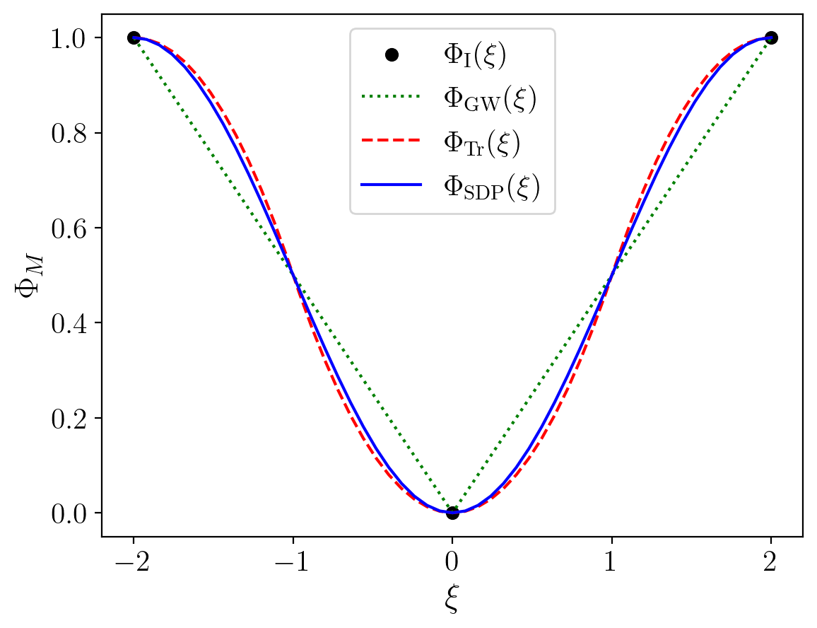
Figure 1: Comparison of core functions of several relaxation-based Ising machines: $\Phi_{\mathrm{I}}$ is the discrete function of the binary Ising model, $\Phi_{\mathrm{SDP}}(\boldsymbol{\xi})$, $\Phi_{\mathrm{Tr}}(\boldsymbol{\xi})$, and $\Phi_{\mathrm{GW}}(\boldsymbol{\xi})$ are the core functions of the rank-$2$ SDP relaxation, the triangular model from Refs. [28, 29], and the GW₂ model investigated in the present paper.

Among different relaxations, we emphasize three. The first one corresponds to the rank-$2$ SDP relaxation, which is given by $\Phi_{\text{SDP}}(\xi)=\left(1-\cos\left(\pi\xi/2\right)\right)/2$. Its piece-wise parabolic continuous approximation yields the model investigated in [28], where it was dubbed the triangular model. Near $\xi=0$ (for $\absolutevalue{\xi}\leq 1$), it is defined by $\Phi_{\text{Tr}}(\xi)=\xi^{2}/2$, and near $\absolutevalue{\xi}=2$ by $\Phi_{\text{Tr}}(\xi)=1-(\absolutevalue{\xi}-2)^{2}/2$. Finally, the model of the main interest of the present paper is given for $\absolutevalue{\xi}\leq 2$ by $\Phi_{\text{GW}}(\xi)=\absolutevalue{\xi}/2$. The core functions of these models are compared in Fig. 1.

3 2D Goemans-Williamson model

3.1 Model definition

Assuming that $-2\leq\xi_{m}\leq 2$, we can write the objective function of the model with the core function $\Phi_{\text{GW}}(\xi)$ as

$$\mathcal{C}_{\text{GW}}(\boldsymbol{\xi})=\frac{1}{4}\sum_{m,n}A_{m,n}\absolutevalue{\xi_{m}-\xi_{n}}_{[-2,2]},$$ (6)

where $\absolutevalue{\ldots}_{[-2,2]}$ is a periodic function with period $P=4$ defined by $\absolutevalue{\xi}_{[-2,2]}=\absolutevalue{\xi}$ for $-2\leq\xi\leq 2$. Alternatively, $\absolutevalue{\ldots}_{[-2,2]}$ can be defined as the distance on a circle with circumference $4$. Such a definition connects $\mathcal{C}_{\text{GW}}(\boldsymbol{\xi})$ with a model based on spins represented by unit two-dimensional vectors $\vec{s}_{m}$:

$$\mathcal{C}_{\text{GW}}(\boldsymbol{s})=\frac{1}{2\pi}\sum_{m,n}A_{m,n}\arccos\left(\vec{s}_{m}\cdot\vec{s}_{n}\right).$$ (7)

Indeed, defining vectors $\vec{s}_{m}$ by their polar angles $\pi\xi_{m}/2$ turns (7) into (6).

A model similar to (7) (with $N$-dimensional $\vec{s}_{m}$) was introduced by Goemans and Williamson in [31], where it appeared naturally as the average value of the cut produced by rounding the SDP solution relatively to random hyperplanes. From this perspective, $\mathcal{C}_{\text{GW}}(\boldsymbol{\xi})$ can be called a 2D Goemans-Williamson (GW₂) model. Respectively, we will call the Ising machine with the dynamics determined by this model simply GW₂-machine.

This model has a property that distinguishes it in the family of dynamical Ising machines. Starting from a non-binary state, the GW₂-machine evolves to a state that trivially rounds to a spin configuration producing a cut at least as large as that obtained by the best rounding of the starting state (see Theorem 3.5). An important consequence of this property is that the GW₂-machine can be used for rounding and simple post-processing of the output of relaxation-based Ising machines, as illustrated by Fig. 2. Therefore, a dynamical system driving the Ising machine can be chosen freely, for instance, on the ground of efficiency to solve particular instances of optimization problems.

Figure 2: A relaxation-based heterogeneous Ising machine returning a binary state. First, a dynamical system based on a relaxation (for instance, rank-2 SDP) is initiated by a generic state. Then, the dynamical core is switched to the GW₂ model, which delivers the optimal rounding of the state obtained during the first stage and performs basic post-processing by small perturbations of the terminal state (see Theorem 3.4).

3.2 Model dynamics

The evolution of the dynamical model realizing the GW₂-machine is governed by $\dot{\boldsymbol{\xi}}=\nabla_{\boldsymbol{\xi}}\mathcal{C}_{\text{GW}}(\boldsymbol{\xi})$, which ensures that $\mathcal{C}_{\text{GW}}(\boldsymbol{\xi})$ monotonously increases with time. Thus, for individual nodes, one has

$$\dot{\xi}_{m}=\sum_{n}A_{m,n}\phi_{\text{GW}}(\xi_{m}-\xi_{n}),$$ (8)

where $\phi_{\text{GW}}(\xi)$ is a periodic function, which inside the period, $\xi\in(-P/2,P/2]$, is defined by $\phi_{\text{GW}}(\xi)=\operatorname{sign}(\xi)/2$ for $\xi\in(-P/2,P/2]$. It must be noted that the dynamics of the GW₂-machine requires special attention at the switching surfaces, $\xi_{m}=\xi_{n}$ for $A_{m,n}\neq 0$, at which $\phi_{\text{GW}}\left(\xi_{m}-\xi_{n}\right)$ is discontinuous. The behavior of discontinuous dynamical systems with switching determined by the dynamical variables is a complex problem (see for reviews Refs. [42, 43]). However, for the GW₂ model the problem significantly simplifies because the dynamics is subject to maximizing $\mathcal{C}_{\text{GW}}(\boldsymbol{\xi})$, which serves as the Lyapunov function. Since the technical details of will obscure the most interesting features of the GW₂ model, which justify a detailed investigation of the model, we limit ourselves to enforcing the convention $\operatorname{sign}(0)=0$. We will provide a rigorous consideration of the GW₂ model within the framework of discontinuous dynamical systems elsewhere.

3.3 Basic properties of terminal states

Starting from the initial state $\boldsymbol{\xi}(0)$, the machine traverses the trajectory $\boldsymbol{\xi}(t|\boldsymbol{\xi}(0))$ until it reaches the terminal state $\boldsymbol{\xi}(\infty|\boldsymbol{\xi}(0))$ characterized by $\dot{\boldsymbol{\xi}}=0$. Thus, the machine’s terminal state is a critical point of $\mathcal{C}_{\text{GW}}(\boldsymbol{\xi})$. In contrast to the machines, whose dynamics is determined by $\mathcal{C}_{\text{SDP}}$ and $\mathcal{C}_{\text{Tr}}$, the GW₂-machine reaches equilibrium in finite time. Indeed, for out-of-equilibrium states, the rate of changing of $\mathcal{C}_{\text{GW}}(\boldsymbol{\xi})$ is limited from below:

$$\frac{d}{dt}\mathcal{C}_{\text{GW}}(\boldsymbol{\xi})=\sum_{m}\left(\frac{\partial\mathcal{C}_{\text{GW}}}{\partial\xi_{m}}\right)^{2}\geq 1.$$ (9)

As a result, the time needed by the GW₂-machine to reach equilibrium is limited from above by $\overline{\mathcal{C}}_{\text{GW}}=\max_{\boldsymbol{\xi}}\mathcal{C}(\boldsymbol{\xi})$.

Using the same argument as in [31], it can be proven that $\overline{\mathcal{C}}_{\text{GW}}=\overline{\mathcal{C}}$, or, in other words, that $\mathcal{C}_{\text{GW}}(\boldsymbol{\xi})$ is an exact relaxation. Indeed, on the one hand, one has $\overline{\mathcal{C}}_{\text{GW}}\geq\overline{\mathcal{C}}$, since the GW₂ model is a relaxation. On the other hand, one can show that $\overline{\mathcal{C}}\geq\overline{\mathcal{C}}_{\text{GW}}$. We observe that the probability for a random point on interval $[-2,2]$ to get between given $\xi_{m}$ and $\xi_{n}$ is $\absolutevalue{\xi_{m}-\xi_{n}}/4$. Thus, $\mathcal{C}_{\text{GW}}(\boldsymbol{\xi})$ can be regarded as the average size of cut obtained by random rounding of $\boldsymbol{\xi}$. Since the size of cut produced by an individual rounding cannot exceed $\overline{\mathcal{C}}$, we find that $\overline{\mathcal{C}}\geq\overline{\mathcal{C}}_{\text{GW}}$.

However, the fact that the global maximum of $\mathcal{C}_{\text{GW}}(\boldsymbol{\xi})$ is the maximum cut of the graph is not sufficient for our purposes, as we are primarily interested in finding the partition delivering (approximately) the maximum cut. Therefore, we need to consider the structure of states of the GW₂-machine.

We notice that $\mathcal{C}_{\text{GW}}(\boldsymbol{\xi})$ is invariant with respect to global translations $\boldsymbol{\xi}\to\boldsymbol{\xi}+a\boldsymbol{1}$, where $a$ is a real number and $(\boldsymbol{1})_{m}=1$. Therefore, we need to identify as binary all states that are obtained by displacing some $\boldsymbol{\sigma}$. Even in view of the extended definition of binary states, the fact that a representation is exact does not imply that all states delivering maxima of $\mathcal{C}_{\text{GW}}$ are binary. It is, therefore, important that the GW₂ model in addition to being exact has a stronger property: critical points of $\mathcal{C}_{\text{GW}}(\boldsymbol{\xi})$ are at least in the same connected manifolds as binary states. Thus, the critical values of $\mathcal{C}_{\text{GW}}$ coincide with possible values of cuts.

Theorem 3.1.

Let $\mathcal{M}\left(c\right)=\left\{\boldsymbol{\xi}\in\mathbb{R}^{N}:\nabla_{\boldsymbol{\xi}}\mathcal{C}_{\text{GW}}(\boldsymbol{\xi})=0,\mathcal{C}_{\text{GW}}(\boldsymbol{\xi})=c\right\}$ be the manifold of critical points corresponding to the same critical value $c$, then each connected component of $\mathcal{M}(c)$ contains a binary state.

Before we turn to the proof of this theorem, we introduce new dynamical variables. Any number $\xi\in\mathbb{R}$ can be uniquely presented as

$$\xi=\sigma+X+4k,$$ (10)

where $\sigma\in\left\{-1,1\right\}$, $X\in(-1,1]$, and $k\in\mathbb{Z}$. The last term, representing multiples of the period of the counting function, will play the minor role, and, therefore, we will also write $\xi=\sigma+X\mod P$.

Using representation (10) in Eq. (6), we can write

$$\mathcal{C}_{\text{GW}}\left(\boldsymbol{\xi}\right)=\mathcal{C}_{\text{GW}}\left(\boldsymbol{\sigma},\mathbf{X}\right):=\mathcal{C}\left(\boldsymbol{\sigma}\right)+\widetilde{\mathcal{C}}_{\text{GW}}\left(\boldsymbol{\sigma},\mathbf{X}\right),$$ (11)

where

$$\widetilde{\mathcal{C}}_{\text{GW}}\left(\boldsymbol{\sigma},\mathbf{X}\right)=\frac{1}{4}\sum_{m,n}A_{m,n}\sigma_{m}\sigma_{n}\absolutevalue{X_{m}-X_{n}}.$$ (12)

Equation (11) can be derived by noticing that

$$\Phi_{\text{GW}}(X_{m}-X_{n}+\sigma_{m}-\sigma_{n})=\frac{1}{2}\left(1-\sigma_{m}\sigma_{n}\right)+\sigma_{m}\sigma_{n}\Phi_{\text{GW}}\left(X_{m}-X_{n}\right).$$ (13)

This equality obviously holds when $\sigma_{m}=\sigma_{n}$. In turn, when $\sigma_{m}-\sigma_{n}=\pm 2$, the equality follows from the symmetry of the counting function $\Phi_{\text{GW}}(x\pm 2)=1-\Phi_{\text{GW}}(x)$. It is worth noting that the counting functions $\Phi_{\text{SDP}}$ and $\Phi_{\text{Tr}}$ also have such a symmetry and, therefore, representations similar to (11) can be obtained for rank-$2$ SDP and triangular model as well. Finally, Eq. (12) is written considering that $\Phi_{\text{GW}}\left(X_{m}-X_{n}\right)=\absolutevalue{X_{m}-X_{n}}/2$.

The equations of motion describing the dynamics of the GW₂-machine in terms of the new variables have the form

$$\dot{X}_{m}=\frac{1}{2}\sum_{n}A_{m,n}\sigma_{m}\sigma_{n}\operatorname{sign}\left(X_{m}-X_{n}\right).$$ (14)

They should be solved while taking into account the topology of the new variables (see Fig. 3). For example, the numerical simulations presented in the next section updated the dynamical variables as described in procedure Update listed in Section 4.

Figure 3: The topology of the representation $\xi=\sigma+X\mod P$. The bold circles represent intervals $(-1,1]$, and the thin lines indicate the transitions at the boundaries of these intervals.

In the new variables, it is apparent that the lack of isolated non-binary critical points is the consequence of the local linearity of $\mathcal{C}_{\text{GW}}(\boldsymbol{\sigma},\mathbf{X})$.

Proof of Theorem 3.1..

Let $\boldsymbol{\xi}$ be a critical point of $\mathcal{C}_{\text{GW}}(\boldsymbol{\xi})$ that is not a displacement of a binary state. In other words, one has $\xi_{m}=\sigma_{m}+X_{m}\mod P$ and not all $X_{m}$ are the same (without loss of generality, we can assume that $X_{m}\neq 1$ for all $m$). We show that $\boldsymbol{\xi}$ can be contracted to a binary state while staying on the critical manifold.

We partition $\mathcal{V}$ by collecting nodes with the same $X_{m}$, so that $\mathcal{V}=\bigcup_{p=1}^{K}\mathcal{V}^{(p)}$, where $\mathcal{V}^{{(p)}}=\left\{m\in\mathcal{V}:\xi_{m}=X^{(p)}+\sigma_{m}\mod P\right\}$. If we enumerate $\mathcal{V}^{(p)}$ in such a way that $X^{(p)}>X^{(q)}$ for $p>q$, we can rewrite Eq. (11) as

$$\mathcal{C}_{\text{GW}}(\boldsymbol{\xi}^{(0)})=\mathcal{C}(\boldsymbol{\sigma})+\frac{1}{2}\sum_{p>q}\sum_{\begin{subarray}{c}m\in\mathcal{V}^{(p)}\\ n\in\mathcal{V}^{(q)}\end{subarray}}A_{m,n}\sigma_{m}\sigma_{n}\left(X^{(p)}-X^{(q)}\right).$$ (15)

With respect to each $X^{(p)}$, this is a linear function, hence, its gradient does not depend on the magnitude of $\mathbf{X}$. Let $\left\{\lambda_{1},\lambda_{2}\ldots\right\}$ with $0<\lambda_{j}<1$ be a Cauchy sequence converging to 0. Since $\lambda_{j}X^{(p)}>\lambda_{j}X^{(q)}$ for $p>q$, the sequence $\boldsymbol{\xi}_{j}=\boldsymbol{\sigma}+\lambda_{j}\mathbf{X}$ is a Cauchy sequence of critical points of $\mathcal{C}_{\text{GW}}$ converging to $\boldsymbol{\sigma}$. ∎

Most of the critical points of $\mathcal{C}_{\text{GW}}$ are saddle points. Their shape is expressed by the homogeneity of $\widetilde{\mathcal{C}}_{\text{GW}}(\boldsymbol{\sigma},\mathbf{X})$:

$$\mathcal{C}_{\text{GW}}(\boldsymbol{\sigma},\lambda\mathbf{X})=\mathcal{C}(\boldsymbol{\sigma})+\absolutevalue{\lambda}\widetilde{\mathcal{C}}_{\text{GW}}(\boldsymbol{\sigma},\mathbf{X}).$$ (16)

It should be noted that while this expression is defined for $\norm{\mathbf{X}}_{\infty}\leq 1$ and $\norm{\lambda\mathbf{X}}_{\infty}\leq 1$, it formally holds for $\absolutevalue{\lambda}\leq\min_{(m,n)\in\mathcal{E}}2/\absolutevalue{X_{m}-X_{n}}$. For example, let $\boldsymbol{\delta}(\boldsymbol{\sigma}^{\prime}|\boldsymbol{\sigma})$ be a $(0,1)$-vector connecting $\boldsymbol{\sigma}$ to $\boldsymbol{\sigma}^{\prime}$ in the $\boldsymbol{\xi}$-space, that is $\delta(\boldsymbol{\sigma}^{\prime}|\boldsymbol{\sigma})_{m}=0$, if $\sigma_{m}^{\prime}=\sigma_{m}$, and $\delta(\boldsymbol{\sigma}^{\prime}|\boldsymbol{\sigma})_{m}=1$, if $\sigma_{m}^{\prime}=-\sigma_{m}$. Then, $\boldsymbol{\sigma}+2\boldsymbol{\delta}(\boldsymbol{\sigma}^{\prime}|\boldsymbol{\sigma})=\boldsymbol{\sigma}^{\prime}\mod P$. Using this relation in (16), we obtain the correct

$$\widetilde{\mathcal{C}}_{\text{GW}}\left(\boldsymbol{\sigma},\boldsymbol{\delta}(\boldsymbol{\sigma}^{\prime}|\boldsymbol{\sigma})\right)=\frac{1}{2}\left[\mathcal{C}(\boldsymbol{\sigma}^{\prime})-\mathcal{C}(\boldsymbol{\sigma})\right].$$ (17)

This relation can be proven directly by noticing that, in terms of $\mathbf{X}(\boldsymbol{\sigma}^{\prime}|\boldsymbol{\sigma})$, the relation between $\boldsymbol{\sigma}^{\prime}$ and $\boldsymbol{\sigma}$ can be written as

$$\sigma_{m}^{\prime}=\sigma_{m}\left(1-2\delta(\boldsymbol{\sigma}^{\prime}|\boldsymbol{\sigma})_{m}\right).$$ (18)

Then, we have the following chain of equalities, where we have omitted the argument of $\boldsymbol{\delta}(\boldsymbol{\sigma}^{\prime}|\boldsymbol{\sigma})$,

$$\begin{split}\mathcal{C}(\boldsymbol{\sigma}^{\prime})-\mathcal{C}(\boldsymbol{\sigma})=&\frac{1}{4}\sum_{m,n}A_{m,n}\left(\sigma_{m}\sigma_{n}-\sigma^{\prime}_{m}\sigma^{\prime}_{n}\right)\\ &=\frac{1}{2}\sum_{m,n}A_{m,n}\sigma_{m}\sigma_{n}\left(\delta_{m}+\delta_{n}-2\delta_{m}\delta_{n}\right)\\ &=\frac{1}{2}\sum_{m,n}A_{m,n}\sigma_{m}\sigma_{n}\left(\delta_{m}-\delta_{n}\right)^{2}\\ &=\frac{1}{2}\sum_{m,n}A_{m,n}\sigma_{m}\sigma_{n}\absolutevalue{\delta_{m}-\delta_{n}}\\ &=2\widetilde{\mathcal{C}}_{\text{GW}}\left(\boldsymbol{\sigma},\boldsymbol{\delta}(\boldsymbol{\sigma}^{\prime}|\boldsymbol{\sigma})\right),\end{split}$$ (19)

where we have taken into account that for $(0,1)$-vectors ${\delta_{m}}^{2}=\delta_{m}$.

It follows from Eq. (14) that for any $\mathbf{Y}\in\mathbb{R}^{N}$ such that $\norm{\mathbf{Y}}_{\infty}\leq 1$ and $\lambda\in\mathbb{R}$ such that $\norm{\lambda\mathbf{Y}}_{\infty}\leq 1$, one has

$$\left.\nabla_{\mathbf{X}}\widetilde{\mathcal{C}}_{\text{GW}}\left(\boldsymbol{\sigma},\mathbf{X}\right)\right|_{\mathbf{X}=\lambda\mathbf{Y}}=\operatorname{sign}(\lambda)\left.\nabla_{\mathbf{X}}\widetilde{\mathcal{C}}_{\text{GW}}\left(\boldsymbol{\sigma},\mathbf{X}\right)\right|_{\mathbf{X}=\mathbf{Y}}.$$ (20)

However, since $\nabla_{\mathbf{X}}\mathcal{C}_{\text{GW}}$ is discontinuous, this does not imply that points $\boldsymbol{\xi}(t)=\boldsymbol{\sigma}+t\boldsymbol{\delta}\left(\sigma^{\prime}|\boldsymbol{\sigma}\right)$ with $0<t<2$, that is lying on the segment connecting $\boldsymbol{\sigma}$ and $\boldsymbol{\sigma}^{\prime}$, are critical. For that, we need a more detailed analysis of the internal structure of the critical points.

The immediate consequence of Eqs. (16) and (17) is

Theorem 3.2.

All binary states, except for max-cut and $\pm\boldsymbol{1}$, are saddle points of $\mathcal{C}_{\text{GW}}(\boldsymbol{\xi})$.

Proof.

Let $\boldsymbol{\sigma}$ be a state with $0<\mathcal{C}(\boldsymbol{\sigma})<\overline{\mathcal{C}}$, then there exist states $\boldsymbol{\sigma}_{\pm}$ such that $\mathcal{C}(\boldsymbol{\sigma}_{-})<\mathcal{C}(\boldsymbol{\sigma})$ and $\mathcal{C}(\boldsymbol{\sigma}_{+})>\mathcal{C}(\boldsymbol{\sigma})$. Functions $C_{\pm}(t)=\mathcal{C}_{\text{GW}}(\boldsymbol{\sigma}+t\boldsymbol{\delta}(\boldsymbol{\sigma}_{\pm}|\boldsymbol{\sigma}))$ are defined on the interval $-2<t<2$ and $t=0$ is the local maximum of $C_{-}(t)$ and the local minimum of $C_{+}(t)$. Hence, $\boldsymbol{\sigma}$ is a saddle point of $\mathcal{C}_{\text{GW}}(\boldsymbol{\xi})$.

A similar argument shows that states $\pm\boldsymbol{1}$ are the only minima and the max-cut states are the only maxima of $\mathcal{C}_{\text{GW}}(\boldsymbol{\xi})$. ∎

3.4 Invariance of the cut size with respect to rounding

The critical points of $\mathcal{C}(\boldsymbol{\xi})$ do not have to be binary, or, in other words, the critical manifold do not have to be the union of isolated points. The presence of non-binary states raises the question about their rounding. As we will show, this question resolves trivially for the GW₂ model written in terms of variables $\boldsymbol{\sigma}$ and $\mathbf{X}$: simple discarding the continuous component $\mathbf{X}$ yields the best rounded state.

We start by noticing that mapping $\widehat{S}:\boldsymbol{\xi}\mapsto(\boldsymbol{\sigma},\mathbf{X})$ factually implements rounding by fixing the reference point for $\boldsymbol{\xi}$. Due to the translational symmetry of $\mathcal{C}_{\text{GW}}(\boldsymbol{\xi})$, the reference point can be freely changed leading to a family of mappings $\widehat{S}_{r}:\boldsymbol{\xi}\mapsto(\boldsymbol{\sigma}(r),\mathbf{X}(r))$ with

$$\xi_{m}-r=\sigma_{m}(r)+X_{m}(r)\mod P.$$ (21)

Using this relation, we define rounding of an arbitrary state $\boldsymbol{\xi}$ with respect to the rounding center $r$ as $\widehat{R}_{r}:\boldsymbol{\xi}\mapsto\boldsymbol{\sigma}(r)$. It suffices to consider $0\leq r<2$, since $\boldsymbol{\sigma}+2=-\boldsymbol{\sigma}\mod P$ and, therefore, $\boldsymbol{\sigma}(r+2)=-\boldsymbol{\sigma}(r)$.

For $0<r<1+\min_{m}X_{m}$, the variation of $r$ leaves both terms in Eq. (11) intact. For larger values of $r$, however, some spins in $\boldsymbol{\sigma}(r)$ are reversed comparing to $\boldsymbol{\sigma}(0)$ and, generally, for an arbitrary non-binary state $\mathcal{C}(\boldsymbol{\sigma}(r))\neq\mathcal{C}(\boldsymbol{\sigma}(0))$. It is, therefore, an important property of the GW₂ model that the size of the cut, produced by rounding a non-binary critical point, does not depend on $r$.

Theorem 3.3.

Let $c$ be a critical value of $\mathcal{C}_{\text{GW}}$, $\mathcal{M}(c)$ be the manifold of critical points yielding $c$, and $\mathcal{S}(c)=\left\{\boldsymbol{\sigma}\in\left\{-1,1\right\}^{N}:\mathcal{C}(\boldsymbol{\sigma})=c\right\}$ be the set of binary states in $\mathcal{M}(c)$. Then, for all $\boldsymbol{\xi}\in\mathcal{M}(c)$, one has $\widehat{R}_{r}[\boldsymbol{\xi}]\in\mathcal{S}(c)$. In other words, rounding a non-binary critical point with respect to different rounding centers produces binary states yielding the same cut.

Proof.

Let $\left\{\mathcal{V}^{(p)}\right\}_{p=1,\ldots,K}$ be a partition of graph nodes $\mathcal{V}$ such that $\mathcal{V}^{(p)}=\left\{m\in\mathcal{V}:\xi_{m}=X^{(p)}+\sigma_{m}\mod P\right\}$ with $X^{(p)}>X^{(q)}$ for $p>q$.

Since $\boldsymbol{\xi}$ is a critical point, $\partial\mathcal{C}_{\text{GW}}(\boldsymbol{\xi})/\partial X^{(p)}=0$ (this is a necessary condition of criticality but not sufficient). Hence, $\mathcal{C}_{\text{GW}}$ is invariant with respect to contracting $\boldsymbol{\xi}$ to $\boldsymbol{\sigma}$: $\mathcal{C}_{\text{GW}}(\boldsymbol{\xi})=\mathcal{C}_{\text{GW}}(\boldsymbol{\sigma},\mathbf{X})=\mathcal{C}_{\text{GW}}(\boldsymbol{\sigma},\lambda\mathbf{X})$ for $0<\lambda<1$. Thus, $\boldsymbol{\sigma}=:\boldsymbol{\sigma}(0)\in\mathcal{S}(c)$.

For $0<r<r_{1}$, where $r_{1}=1+X^{(1)}$, one has $\boldsymbol{\sigma}(r)=\boldsymbol{\sigma}(0)$ and $X^{(p)}(r)=X^{(p)}-r$. At $r=r_{1}$, spins at nodes in $\mathcal{V}^{(1)}$ are inverted: $\sigma_{m}(r_{1})=-\sigma_{m}(0)$ for all $m\in\mathcal{V}^{(1)}$. This changes the rounded state, but the cut produced by the new state is the same.

Indeed, expanding $\partial\mathcal{C}_{\text{GW}}(\boldsymbol{\xi})/\partial X^{(1)}=0$ (see Eq. (15)) produces

$$-\sum_{m\in\mathcal{V}^{(1)}}\sum_{n\notin\mathcal{V}^{(1)}}A_{m,n}\sigma_{m}\sigma_{n}=0.$$ (22)

This relation is invariant with respect to transformation $\sigma_{m}\to-\sigma_{m}$ for all $m\in\mathcal{V}^{(1)}$. Thus, inverting spins in $\mathcal{V}^{(1)}$ does not change the total cut.

For $r_{1}<r<r_{2}:=1+X^{(2)}$, we have $\boldsymbol{\sigma}(r)=\boldsymbol{\sigma}(r_{1})$ and $X^{(2)}(r)<\ldots<X^{(K)}(r)<X^{(1)}(r)$. At $r=r_{2}$, spins in $\mathcal{V}^{(2)}$ are inversed. The same argument as above shows that this inversion does not change the cut size.

This process, increasing $r$ and inverting spins in $\mathcal{V}^{(i)}$ at $r=r_{i}:=1+X^{(i)}$, continues until $r$ reaches $r_{K}$. At this point, one obtains $\boldsymbol{\sigma}(r_{K})=-\boldsymbol{\sigma}(0)$ and the same mutual relations between $X^{(p)}\left(r_{K}\right)$ as between $X^{(p)}\left(0\right)$. Thus, while increasing $r$, rounding $\widehat{R}_{r}[\boldsymbol{\xi}]$ produces the periodic sequence of binary states $\left\{\boldsymbol{\sigma}(0),\boldsymbol{\sigma}(r_{1}),\ldots,\boldsymbol{\sigma}(r_{K-1}),-\boldsymbol{\sigma}(0),-\boldsymbol{\sigma}(r_{1}),\ldots,-\boldsymbol{\sigma}(r_{K-1}),\boldsymbol{\sigma}(0),\ldots\right\}$. All these states are in $\mathcal{S}(c)$.

To complete the proof, one needs to show that one does not need to increase the rounding center gradually and that $\widehat{R}_{r}[\boldsymbol{\xi}]=\boldsymbol{\sigma}(r_{i})$ for $r_{i}\leq r<r_{i+1}$. Indeed, in this case, $\boldsymbol{\sigma}(r)$ is obtained from $\boldsymbol{\sigma}(0)$ by inverting spins in $\mathcal{V}^{(1,i)}=\bigcup_{p\leq i}\mathcal{V}^{(i)}$, which yields $\boldsymbol{\sigma}(r_{i})$ since $\mathcal{V}^{(p)}$ are mutually disjoint. ∎

It follows from Theorem 3.3 that for a critical point $\boldsymbol{\xi}$ of $\mathcal{C}_{\text{GW}}$, the notion of cut is correctly defined even if $\boldsymbol{\xi}$ is not binary: $\mathcal{C}(\boldsymbol{\xi}):=\mathcal{C}\left(\widehat{R}[\boldsymbol{\xi}]\right)$, where $\widehat{R}[\boldsymbol{\xi}]$ is an arbitrary rounding.

Also, it should be noted that Theorem 3.3 is the most sensitive to regularizations of $\mathcal{C}_{\text{GW}}(\boldsymbol{\xi})$ as mapping $\widehat{R}_{r}[\boldsymbol{\xi}]$ may not be well-defined for $x=X_{p}$. In this case, for the regularized objective function, Theorem 3.3 holds for almost all points in critical manifold $\mathcal{M}(c)$.

3.5 Non-decreasing cuts and optimal rounding

As discussed above, rounding of non-critical states produces cuts of size depending on the choice of the rounding center. For instance, this is the typical situation for equilibrium states of machines based on rank-2 SDP. Therefore, the problem of recovering the best rounding of such states needs to be specifically addressed. The main result of our theoretical analysis of the GW₂ model in the present paper is that the GW₂-machine, by design, delivers such rounding. This follows from the observation that dynamics $\boldsymbol{\xi}(t)$ does not depend on the choice of the rounding center and an essential property of the GW₂-machine that (small) perturbations of binary states cannot reduce the cut.

Theorem 3.4.

Let a binary state $\boldsymbol{\sigma}$ be perturbed by $\mathbf{X}\in(-1,1]^{N}$, then the terminal machine’s state yields cut of at least the same size as in the initial state:

$$\mathcal{C}\left(\boldsymbol{\xi}\left(\infty|\boldsymbol{\sigma}+\mathbf{X}\right)\right)\geq\mathcal{C}(\boldsymbol{\sigma}).$$ (23)

Proof.

There are two mutually excluding scenarios of how the machine may evolve.

The first scenario is when none of $X_{m}$, $m=1,\ldots,N$, crosses $-1$ or $1$, so that $\boldsymbol{\sigma}(t)=\boldsymbol{\sigma}$. Then, by virtue of Theorem 3.3, the terminal state has the same cut as $\boldsymbol{\sigma}$.

The second scenario occurs when one of $\left\{X_{m}\right\}$, say, $X_{p}$, passes through $-1$ or $1$ leading to inverting the spin, $\sigma_{p}\to-\sigma_{p}$. As will be shown below, the new state has the cut strictly larger than $\mathcal{C}(\boldsymbol{\sigma})$. For the new state, we again have dynamics of a perturbed binary state. This dynamics also proceeds according to one of the two scenarios and so on. Since the total variation of cut is finite, $\boldsymbol{\sigma}$ may change only a finite number of times. Thus, the evolution arrives at the terminal state without decreasing the cut size.

To complete the proof, we must show that the binary component may change only by increasing the cut. We consider the case when the variation occurs at crossing $-1$. Let $X_{p}$ be the component, which is about to cross $-1$, that is $X_{p}=\min_{m}X_{m}$ and $\dot{X}_{p}<0$. Expanding Eq. (14), we obtain

$$\dot{X}_{p}=-\frac{1}{2}\sum_{n}A_{p,n}\sigma_{p}\sigma_{n}.$$ (24)

Hence, $\dot{X}_{p}<0$ only if $F(p)>0$ (see Eq. (4)) and, therefore, inverting $\sigma_{p}$ increases the cut. The same conclusion holds when crossing occurs at $1$, or when a group of spins characterized by $X_{m}=X^{(p)}$ crosses $-1$ or $1$. ∎

This property, weak perturbations do not decrease (by the time when the terminal state is reached) the cut, is a distinguishing feature of the GW₂-machine. For example, the machine based on rank-2 SDP does not have this property. For such a machine, perturbing a binary state may lead to a reduced cut.

Finally, applying these results to the progression of a non-critical state, we obtain our main result. Starting from an arbitrary state, the GW₂-machine terminates in a state with cut, which is not worse than produced by the best rounding of the initial state.

Theorem 3.5.

Let the machine be initially in a non-critical state $\boldsymbol{\xi}^{(0)}$ with $\overline{\mathcal{C}}\left(\boldsymbol{\xi}^{(0)}\right)$ being the maximum cut that can be obtained by rounding it, and let $\boldsymbol{\xi}\left(\infty|\boldsymbol{\xi}^{(0)}\right)$ be the machine terminal state, then

$$\mathcal{C}\left(\boldsymbol{\xi}\left(\infty|\boldsymbol{\xi}^{(0)}\right)\right)\geq\overline{C}\left(\boldsymbol{\xi}^{(0)}\right).$$ (25)

Proof.

Since choosing the rounding center does not change $\mathcal{C}_{\text{GW}}\left(\boldsymbol{\xi}(t)\right)$, we can consider the dynamics as emerging from the perturbation of the best rounding state. Then, by virtue of Theorem 3.4, the cut cannot decrease. ∎

4 Computational performance of the GW₂-machine

The computational effort of the Ising machine driven by the GW₂ model during the final stage (Fig. 2) is represented by terminal states of the GW₂ model: $\boldsymbol{\xi}\left(\infty|\boldsymbol{\xi}(0)\right)$, where $\boldsymbol{\xi}(0)$ is the machine state at the start of the GW₂ stage. A proper investigation of the evolution of probability distributions on the phase space is a logical next step in studying the computational properties of the GW₂ model. However, it requires developing special approaches, which are beyond the scope of the present paper. Therefore, we limit ourselves to a numerical demonstration of model’s computational capabilities, while taking into consideration the results obtained in the previous section.

In presented numerical experiments, the machine state is described by variables $(\boldsymbol{\sigma},\mathbf{X})$ with the update rule implemented using procedure Update listed below. The dynamics of the GW₂ model was simulated using the Euler approximation. This approximation is exact as long as the system does not pass through the discontinuities of the dynamical equations (8) or (14). On the other hand, since the magnitude of $\dot{\boldsymbol{\xi}}$ does not depend on the proximity to equilibrium, the Euler approximation with a fixed time step demonstrates spurious oscillations near the critical point as characteristic to discontinuous dynamical systems (see, e.g. [44]). As suggested by the results of the previous section, reaching equilibrium is important for the solution quality because, otherwise, one cannot ensure that Theorems 3.3, 3.4, 3.5 hold. Consequently, these spurious oscillations are expected to negatively impact the performance of the GW₂-machine. On the other hand, the Euler approximation effectively selects a regularization of $\mathcal{C}_{\text{GW}}(\boldsymbol{\xi})$, which alleviates difficulties associated with discontinuities of the dynamical equations of motion. From this perspective, the numerical results presented below demonstrate the robustness of the favorable features of the GW₂ model with respect to realizations of discontinuous dynamics.

procedure Update(input $\left(\boldsymbol{\sigma},\mathbf{X}\right)$, $\Delta\mathbf{X}$; output $\left(\boldsymbol{\sigma},\mathbf{X}\right)$)

$\norm{\Delta\mathbf{X}}_{\infty}<2$

     $\mathbf{X}\leftarrow\mathbf{X}+\Delta\mathbf{X}$

     for all $m\in 1,\dots,N$ do

         if $X_{m}>1$ then

              $X_{m}\leftarrow X_{m}-2$

              $\sigma_{m}\leftarrow-\sigma_{m}$

         else if $X_{m}\leq-1$ then

              $X_{m}\leftarrow X_{m}+2$

              $\sigma_{m}\leftarrow-\sigma_{m}$

         end if

     end for

end procedure

To improve the convergence to equilibrium and to utilize the non-worsening property, the GW₂ stage was repeated $50$ times. After each iteration, the continuous component was discarded and randomly reinitialized. Additionally, the duration of the simulation was increased, while the time step was decreased. A systematic study of the effect of hyperparameters, such as the running time and the time step, is a subject of ongoing research. It is worth emphasizing that this simple way to address the spurious oscillations near equilibrium already shows good performance.

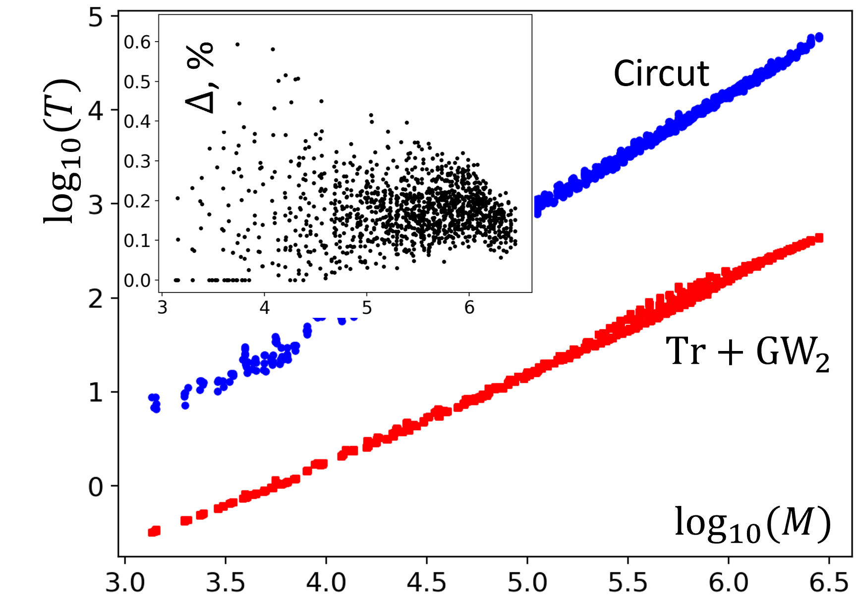
Figure 4: Comparison of a heterogeneous $\Phi_{\text{Tr}}/\Phi_{\text{GW}}$ machine (see Fig. 2) with Circut on random Erdős-Rényi graphs. The main panel plots the dependence of the running time ($\log_{10}(T)$ with $T$ measured in seconds) on the number of edges in the graph, the inset shows the discrepancy between the values of cuts obtained by different methods: $\Delta=2(\mathcal{C}_{\mathtt{Circut}}-\mathcal{C}_{\text{GW}})/(\mathcal{C}_{\mathtt{Circut}}+\mathcal{C}_{\text{GW}})\times 100\%$.

An important property of the GW₂ model is its ability to perform optimal rounding of a state obtained by a relaxation-based Ising machine. In Fig. 4, we consider a heterogeneous Ising machine that, first, is governed by $\Phi_{\text{Tr}}$ (defined in Section 2) and, then, is switched to the GW₂ model. In what follows, however, we will concentrate on the GW₂-machine alone, initialized in a random non-binary state.

Figure 4 compares the heterogeneous (as outlined in Fig. 2) $\Phi_{\text{Tr}}/\Phi_{\text{GW}}$ Ising machine to Circut, a rank-2 SDP-based solver [32]. The comparison is done on a family of random Erdős-Rényi (ER) graphs $\mathcal{G}(N,p)$, where $p$ is the probability for an edge to be present. In the simulation, $N$ varied from $50$ to $4000$, and $p$ was changing from $0.05$ to $0.35$.

This simulation shows that the Ising machine running time scales as $\mathcal{O}(N^{2})$ owing to the number of edges in the random ER graphs being proportional to $N^{2}$ and the fixed number of time steps. Because of the slower increase of the running time, the Ising machine on medium-sized graphs can obtain a solution significantly faster than Circut with an error under one percent. Similar results are obtained for the GW₂-machine running alone, as shown in Fig. 5(a). It must be emphasized that in all presented simulations, the Ising machines ran unsupervised besides random perturbations after each iteration and did not employ any post-processing, for example, selecting the best solution from a set obtained, say, by starting from different initial conditions.

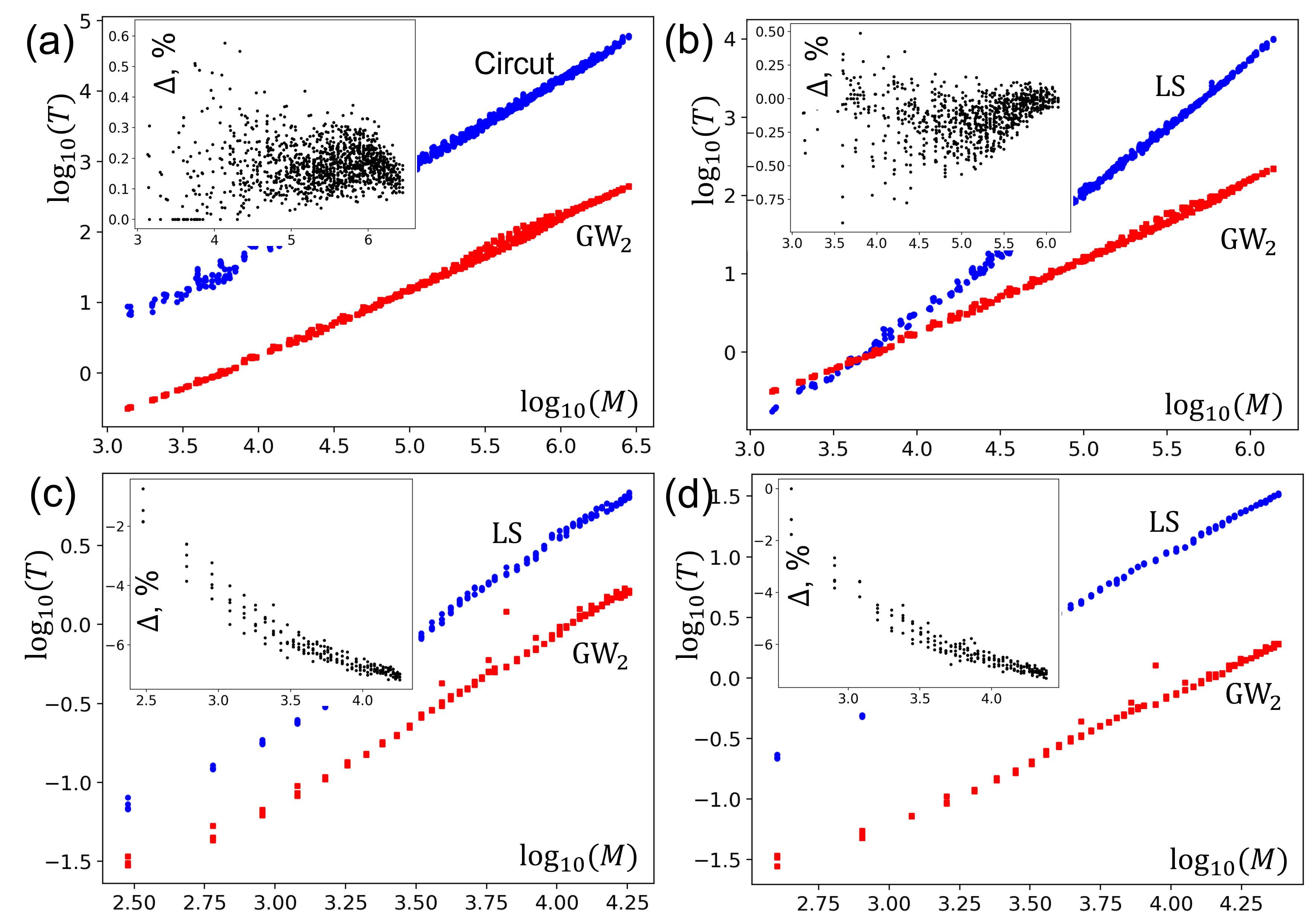
Figure 5: Comparison of the performance of the GW₂-machine with Circut (a) and the $2$-opt local search (b-d) on families of random graphs: (a, b) Erdős-Rényi, (c) $3$-regular, (c) $4$-regular. The main panels plot the running time ($\log_{10}(T)$ with $T$ measured in seconds) versus the number of edges in the graphs. The insets show the discrepancy $\Delta=2(\mathcal{C}_{X}-\mathcal{C}_{\text{GW}})/(\mathcal{C}_{X}+\mathcal{C}_{\text{GW}})\times 100\%$, where $X$ stands for LS or Circut. The outliers in (c) and (d) are due to restarted GW₂-machine and the impact of the Julia compilation time.

Besides delivering the optimal rounding, the GW₂-machine can also perform certain post-processing owing to the ability to improve the solution without losing the quality of the already obtained one. To illustrate this feature, we compare, in Figs. 5(b)-(d), the GW₂-machine with the $2$-opt local search. This local search ensures that reverting up to two spins cannot improve the cut, or, in other words, there are no improving cut partitions within Hamming distance two. The local search was performed in two steps. First, the standard $1$-opt local search was used to obtained $\boldsymbol{\sigma}$ such that $F_{m}(\boldsymbol{\sigma})\leq 0$ for all $m$. Then, for all cut edges $(m,n)$, it was ensured that $F_{m}(\boldsymbol{\sigma})+F_{n}(\boldsymbol{\sigma})\leq-2$. For each graph, the procedure was repeated $1,000$ times starting from a random initial state. As the final result, the best out of $1,000$ obtained cuts is taken.

The obtained numerical results indicate that, at least for the considered families of graphs, the GW₂ model can regularly outperform the local search either by delivering solutions of better quality or, when the solution quality is comparable, by showing better scaling with the problem size.

5 Conclusion

The connection between the ground state of the classical spin system and the max-cut problem provides means for evaluating and projecting the computational capabilities of Ising machines, for instance, how their performance will scale with the problem size. In recent papers [26, 28, 29], we approached the problem of designing Ising machines from the perspective of employing dynamical models inspired by relaxation-based techniques, such as the SDP relaxation. These techniques are known to demonstrate favorable scaling properties. However, the respective dynamical systems settle in a non-binary state, and the final state must be rounded to recover a feasible solution to the Ising or max-cut problem. The known rounding algorithms, even in the case of rank-2 relaxations, associating spins with planar unit vectors, require external processing power. This makes the information processing flow in relaxation-based Ising machines incomplete.

We show that a special dynamical model (we call it GW₂ model) possesses the key property: given a non-binary initial state, it evolves towards a trivially rounding state, which yields the cut that, at least, is not smaller than obtained by the best rounding of the initial state.

Another important property of the GW₂ model is tightly related to the ability to deliver the best rounding. We show that if the GW₂ model evolves from a slight perturbation of a binary state, it ends up in a state producing a cut not smaller than that of the original binary state, which enables improving the solution quality. We compare numerically the GW₂-machine with the $2$-opt local search on several families of random graphs (Erdős-Rényi, $3$- and $4$-regular) and show that the GW₂-machine delvers solution of, at least, comparable quality, while scaling slower with the problem size.

Thus, incorporating the GW₂ model as the final stage of a heterogeneous Ising machine eliminates the necessity for the external processing of relaxation-based Ising machines and makes them self-contained. Consequently, any dynamical system with the phase space consistent with the GW₂ model can be used to drive the Ising machine and can be chosen solely on the ground of computational performance on particular instances of optimization problems.

References

- [1] S. Kirkpatrick, C. D. Gelatt, M. P. Vecchi, Optimization by Simulated Annealing, Science 220 (4598) (1983) 671–680. doi:10.1126/science.220.4598.671.
- [2] J. J. Hopfield, Neurons with graded response have collective computational properties like those of two-state neurons., Proceedings of the National Academy of Sciences 81 (10) (1984) 3088–3092. doi:10.1073/pnas.81.10.3088.
- [3] V. Černý, Thermodynamical approach to the traveling salesman problem: An efficient simulation algorithm, Journal of Optimization Theory and Applications 45 (1) (1985) 41–51. doi:10.1007/BF00940812.
- [4] Y. Fu, P. W. Anderson, Application of statistical mechanics to NP-complete problems in combinatorial optimisation, Journal of Physics A: Mathematical and General 19 (9) (1986) 1605–1620. doi:10.1088/0305-4470/19/9/033.
- [5] G. A. Kochenberger, F. Glover, H. Wang, Binary Unconstrained Quadratic Optimization Problem, in: P. M. Pardalos, D.-Z. Du, R. L. Graham (Eds.), Handbook of Combinatorial Optimization, Springer, New York, NY, 2013, pp. 533–557. doi:10.1007/978-1-4419-7997-1_15.
- [6] F. Barahona, On the computational complexity of Ising spin glass models, Journal of Physics A: Mathematical and General 15 (10) (1982) 3241–3253. doi:10.1088/0305-4470/15/10/028.
- [7] R. M. Karp, Reducibility among Combinatorial Problems, in: R. E. Miller, J. W. Thatcher, J. D. Bohlinger (Eds.), Complexity of Computer Computations, Springer US, Boston, MA, 1972, pp. 85–103. doi:10.1007/978-1-4684-2001-2_9.
- [8] M. Garey, D. Johnson, L. Stockmeyer, Some simplified NP-complete graph problems, Theoretical Computer Science 1 (3) (1976) 237–267. doi:10.1016/0304-3975(76)90059-1.
- [9] A. Lucas, Ising formulations of many NP problems, Frontiers in Physics 2 (2014) 5. doi:10.3389/fphy.2014.00005.
- [10] N. A. Aadit, A. Grimaldi, M. Carpentieri, L. Theogarajan, J. M. Martinis, G. Finocchio, K. Y. Camsari, Massively parallel probabilistic computing with sparse Ising machines, Nature Electronics 5 (7) (2022) 460–468. doi:10.1038/s41928-022-00774-2.
- [11] K. Tatsumura, Large-scale combinatorial optimization in real-time systems by FPGA-based accelerators for simulated bifurcation, in: Proceedings of the 11th International Symposium on Highly Efficient Accelerators and Reconfigurable Technologies, ACM, Online Germany, 2021, pp. 1–6. doi:10.1145/3468044.3468045.
- [12] K. Tatsumura, M. Yamasaki, H. Goto, Scaling out Ising machines using a multi-chip architecture for simulated bifurcation, Nature Electronics 4 (3) (2021) 208–217. doi:10.1038/s41928-021-00546-4.
- [13] S. Patel, P. Canoza, S. Salahuddin, Logically synthesized and hardware-accelerated restricted Boltzmann machines for combinatorial optimization and integer factorization, Nature Electronics 5 (2) (2022) 92–101. doi:10.1038/s41928-022-00714-0.
- [14] K. Yamamoto, K. Kawamura, K. Ando, N. Mertig, T. Takemoto, M. Yamaoka, H. Teramoto, A. Sakai, S. Takamaeda-Yamazaki, M. Motomura, STATICA: A 512-Spin 0.25M-Weight Annealing Processor With an All-Spin-Updates-at-Once Architecture for Combinatorial Optimization With Complete Spin–Spin Interactions, IEEE Journal of Solid-State Circuits 56 (1) (2021) 165–178. doi:10.1109/JSSC.2020.3027702.
- [15] M. Yamaoka, C. Yoshimura, M. Hayashi, T. Okuyama, H. Aoki, H. Mizuno, A 20k-Spin Ising Chip to Solve Combinatorial Optimization Problems With CMOS Annealing, IEEE Journal of Solid-State Circuits 51 (1) (2016) 303–309. doi:10.1109/JSSC.2015.2498601.
- [16] I. Ahmed, P.-W. Chiu, W. Moy, C. H. Kim, A Probabilistic Compute Fabric Based on Coupled Ring Oscillators for Solving Combinatorial Optimization Problems, IEEE Journal of Solid-State Circuits (2021) 1–1doi:10.1109/JSSC.2021.3062821.
- [17] W. Moy, I. Ahmed, P.-w. Chiu, J. Moy, S. S. Sapatnekar, C. H. Kim, A 1,968-node coupled ring oscillator circuit for combinatorial optimization problem solving, Nature Electronics 5 (5) (2022) 310–317. doi:10.1038/s41928-022-00749-3.
- [18] R. Afoakwa, Y. Zhang, U. K. R. Vengalam, Z. Ignjatovic, M. Huang, BRIM: Bistable Resistively-Coupled Ising Machine, in: 2021 IEEE International Symposium on High-Performance Computer Architecture (HPCA), IEEE, Seoul, Korea (South), 2021, pp. 749–760. doi:10.1109/HPCA51647.2021.00068.
- [19] T. Leleu, F. Khoyratee, T. Levi, R. Hamerly, T. Kohno, K. Aihara, Scaling advantage of chaotic amplitude control for high-performance combinatorial optimization, Communications Physics 4 (1) (2021) 266. doi:10.1038/s42005-021-00768-0.
- [20] Y. Kuramoto, Self-entrainment of a population of coupled non-linear oscillators, in: H. Araki (Ed.), International Symposium on Mathematical Problems in Theoretical Physics, Vol. 39, Springer-Verlag, Berlin/Heidelberg, 1975, pp. 420–422. doi:10.1007/BFb0013365.
- [21] S. Shinomoto, Y. Kuramoto, Phase Transitions in Active Rotator Systems, Progress of Theoretical Physics 75 (5) (1986) 1105–1110. doi:10.1143/PTP.75.1105.
- [22] H. Mori, Y. Kuramoto, Dissipative Structures and Chaos, Springer, Berlin ; New York, 1998.
- [23] J. A. Acebrón, L. L. Bonilla, C. J. Pérez Vicente, F. Ritort, R. Spigler, The Kuramoto model: A simple paradigm for synchronization phenomena, Reviews of Modern Physics 77 (1) (2005) 137–185. doi:10.1103/RevModPhys.77.137.
- [24] T. Wang, L. Wu, P. Nobel, J. Roychowdhury, Solving combinatorial optimisation problems using oscillator based Ising machines, Natural Computing (May 2021). doi:10.1007/s11047-021-09845-3.
- [25] T. Wang, J. Roychowdhury, OIM: Oscillator-Based Ising Machines for Solving Combinatorial Optimisation Problems, in: I. McQuillan, S. Seki (Eds.), Unconventional Computation and Natural Computation, Vol. 11493, Springer International Publishing, Cham, 2019, pp. 232–256. doi:10.1007/978-3-030-19311-9_19.
- [26] M. Erementchouk, A. Shukla, P. Mazumder, On computational capabilities of Ising machines based on nonlinear oscillators, Physica D: Nonlinear Phenomena 437 (2022) 133334. doi:10.1016/j.physd.2022.133334.
- [27] F. Böhm, T. V. Vaerenbergh, G. Verschaffelt, G. Van der Sande, Order-of-magnitude differences in computational performance of analog Ising machines induced by the choice of nonlinearity, Communications Physics 4 (1) (2021) 149. doi:10.1038/s42005-021-00655-8.
- [28] A. Shukla, M. Erementchouk, P. Mazumder, Scalable almost-linear dynamical Ising machines (May 2022). arXiv:2205.14760, doi:10.48550/arXiv.2205.14760.
- [29] A. Shukla, M. Erementchouk, P. Mazumder, Cut-maximization using relaxed burer-monteiro heuristics on custom cmos (2022).
- [30] M. X. Goemans, D. P. Williamson, .879-approximation algorithms for MAX CUT and MAX 2SAT, in: Proceedings of the Twenty-Sixth Annual ACM Symposium on Theory of Computing - STOC ’94, ACM Press, Montreal, Quebec, Canada, 1994, pp. 422–431. doi:10.1145/195058.195216.
- [31] M. X. Goemans, D. P. Williamson, Improved approximation algorithms for maximum cut and satisfiability problems using semidefinite programming, Journal of the ACM 42 (6) (1995) 1115–1145. doi:10.1145/227683.227684.
- [32] S. Burer, R. D. C. Monteiro, Y. Zhang, Rank-Two Relaxation Heuristics for MAX-CUT and Other Binary Quadratic Programs, SIAM Journal on Optimization 12 (2) (2002) 503–521. doi:10.1137/S1052623400382467.
- [33] P. Raghavendra, Optimal algorithms and inapproximability results for every CSP?, in: Proceedings of the Fortieth Annual ACM Symposium on Theory of Computing, STOC ’08, Association for Computing Machinery, New York, NY, USA, 2008, pp. 245–254. doi:10.1145/1374376.1374414.
- [34] S. Khot, G. Kindler, E. Mossel, R. O’Donnell, Optimal Inapproximability Results for Max-Cut and Other 2-Variable CSPs?, in: 45th Annual IEEE Symposium on Foundations of Computer Science, IEEE, Rome, Italy, 2004, pp. 146–154. doi:10.1109/FOCS.2004.49.
- [35] S. Burer, R. D. Monteiro, Local Minima and Convergence in Low-Rank Semidefinite Programming, Mathematical Programming 103 (3) (2005) 427–444. doi:10.1007/s10107-004-0564-1.
- [36] S. Burer, R. D. Monteiro, A nonlinear programming algorithm for solving semidefinite programs via low-rank factorization, Mathematical Programming 95 (2) (2003) 329–357. doi:10.1007/s10107-002-0352-8.
- [37] N. Boumal, V. Voroninski, A. S. Bandeira, The non-convex Burer–Monteiro approach works on smooth semidefinite programs, in: 30 Th Conf. Neural Information Processing Systems (NIPS 2016), Barcelona, Spain, 2016, p. 10.
- [38] N. Boumal, V. Voroninski, A. S. Bandeira, Deterministic Guarantees for Burer-Monteiro Factorizations of Smooth Semidefinite Programs, Communications on Pure and Applied Mathematics 73 (3) (2020) 581–608. doi:10.1002/cpa.21830.
- [39] A. S. Bandeira, N. Boumal, V. Voroninski, On the low-rank approach for semidefinite programs arising in synchronization and community detection, in: V. Feldman, A. Rakhlin, O. Shamir (Eds.), 29th Annual Conference on Learning Theory, Vol. 49 of Proceedings of Machine Learning Research, PMLR, Columbia University, New York, New York, USA, 2016, pp. 361–382.
- [40] I. Dunning, S. Gupta, J. Silberholz, What Works Best When? A Systematic Evaluation of Heuristics for Max-Cut and QUBO, INFORMS Journal on Computing 30 (3) (2018) 608–624. doi:10.1287/ijoc.2017.0798.
- [41] A. P. Punnen (Ed.), The Quadratic Unconstrained Binary Optimization Problem. Theory, Algorithms, and Applications, Springer Nature Switzerland AG, Gewerbestrasse, Switzerland, 2022.
- [42] A. F. Filippov, Differential equations with discontinuous righthand sides, Kluwer Academic Publishers, Dordrecht [Netherlands] ; Boston, 1988.
- [43] J. Cortes, Discontinuous dynamical systems, IEEE Control Systems Magazine 28 (3) (2008) 36–73. doi:10.1109/MCS.2008.919306.
- [44] N. Guglielmi, E. Hairer, An efficient algorithm for solving piecewise-smooth dynamical systems, Numerical Algorithms 89 (3) (2022) 1311–1334. doi:10.1007/s11075-021-01154-1.