Sequ

A fluctuation-dissipation relation in a non-equilibrium quantum fluid

Abstract

There is no simple fluctuation-dissipation theorem (FDT) for nonequilibrium systems. We show that for a fluid in a non-equilibrium steady state (NESS) characterized by a constant temperature gradient there is a generalized FDT that relates commutator correlation functions to the bilinear response of products of observables. This allows for experimental probes of the long-range correlations in such a system, quantum or classical, via response experiments. We also show that the correlations are not tied to thermal fluctuations but are intrinsic to the NESS and reflect a generalized rigidity.

A fundamental result of equilibrium statistical mechanics is the fluctuation-dissipation theorem, which states that the system’s linear response to an external perturbation is related to the fluctuations in the equilibrium state Nyquist [1928], Callen and Welton [1951]. Specifically, the response functions are proportional to the corresponding correlation functions, and in a classical system the proportionality factor is simply the inverse temperature Forster [1975]. In a non-equilibrium system this is no longer true. There is a substantial body of work on the properties of fluctuations far from equilibrium (see, e.g., Refs. Sevick et al., 2008, Gaspard, 2022 and references therein), on linear response in non-equilibrium systems Baiesi and Maes [2013], and on aspects of relations between the two Andrieux and Gaspard [2004], Maes [2020], Gaspard [2022], but there is no general prescription for probing fluctuations via the response to external perturbations. Consequently, fluctuations can be observed only via scattering experiments, which become increasingly difficult as the temperature is lowered, but not via the linear response to a macroscopic perturbation. One of the main results reported in this Letter is that for a fluid, classical or quantum, in a non-equilibrium steady state (NESS) characterized by a fixed temperature gradient there still is a relation between fluctuations and response, but it is not linear. Rather, the non-equilibrium parts of the correlation functions determine the bilinear response of products of observables to external perturbations, as we will demonstrate in Eqs. (14) and (18) below. Since perturbations can be controlled experimentally independent of other parameters, this opens new avenues for observing correlations, especially in quantum fluids, where thermal fluctuations are weak due to the low temperature. In addition, we elucidate several other aspects of fluids in such a NESS, especially in the quantum limit.

To motivate our investigations we recall that classical simple fluids subject to a fixed temperature gradient harbor correlations that are extraordinarily long-ranged Kirkpatrick et al. [1982a], Dorfman et al. [1994], Ortiz de Zárate and Sengers [2007]. For instance, the equal-time temperature-temperature correlation function diverges for small wave numbers $k$ as $1/k^{4}$. In real space, this corresponds to correlations that extend over the entire width of the sample and decay on the same scale Ortiz de Zárate and Sengers [2007]. These correlations are generic in the sense that they do not require any fine tuning of parameters, and they are not related to any broken symmetry. Rather, they are the result of the coupling of the temperature fluctuations to the diffusive shear velocity. This surprising result has been confirmed theoretically by means of a variety of techniques Kirkpatrick et al. [1982b], Ronis and Procaccia [1982], Ortiz de Zárate and Sengers [2007], and it has been observed by many light scattering experiments, see Ref. Sengers et al. [2016] and references therein.

Despite being well established and confirmed, this phenomenon raises several questions that historically have not been emphasized. One is the fact, mentioned above, that the relevant correlation functions in a NESS are not in any obvious way related to response functions. Another question is whether the long-ranged correlations are tied to thermal fluctuation effects, or whether they are more generic and reflect some type of generalized rigidity Anderson [1984] that is present even in the zero-temperature limit and also manifests itself in the response of the system to external perturbations. Recent work on classical fluids has suggested the latter Kirkpatrick et al. [2021], but a relation between correlation functions and response theory has been lacking. Part of the purpose of this Letter is to provide such a relation.

The missing correlation-response relation discussed above is equally relevant for classical and quantum fluids, but it poses a particularly significant problem for the latter qua . Direct measurements of the correlation functions via light scattering are difficult even in the classical case because of the very small scattering angles required. With decreasing temperature the fluctuations become smaller, which makes it even more desirable to observe the effect via response experiments, if feasible. Specifically, there are two obvious types of correlation functions: symmetrized, or anticommutator correlation functions that we denote by $S^{\text{sym}}$, and anti-symmetrized, or commutator ones that we denote by $\chi^{\prime\prime}$ (this is the customary notation for the commutator correlation function Forster [1975], with the double prime indicating that this is the spectrum, or spectral density, of a causal function). As functions of the wave vector ${\bm{k}}$ and the frequency $\omega$ they are defined by Forster [1975], cla

$$\frac{1}{2}\,\left\langle\left[\delta{\hat{A}}({\bm{k}}_{1},\omega_{1}),\delta{\hat{B}}({\bm{k}}_{2},\omega_{2})\right]_{+}\right\rangle = V\delta_{{\bm{k}}_{1},-{\bm{k}}_{2}}\,2\pi\delta(\omega_{1}+\omega_{2})\,S^{\text{sym}}_{AB}({\bm{k}}_{1},\omega_{1})\ ,$$ (1a)

$$\frac{1}{2\hbar}\,\left\langle\left[\delta{\hat{A}}({\bm{k}}_{1},\omega_{1}),\delta{\hat{B}}({\bm{k}}_{2},\omega_{2})\right]_{-}\right\rangle = V\delta_{{\bm{k}}_{1},-{\bm{k}}_{2}}\,2\pi\delta(\omega_{1}+\omega_{2})\,\chi_{AB}^{\prime\prime}({\bm{k}}_{1},\omega_{1})\ .$$ (1b)

Here $\delta\hat{A}$, $\delta\hat{B}$ are operator-valued fluctuations of observables, $[\ ,\ ]_{+}$ and $[\ ,\ ]_{-}$ denote anticommutators and commutators, respectively, $\langle\ldots\rangle$ denotes a quantum mechanical expectation value plus a statistical mechanics average, and $V$ is the system volume. We use carets to denote operator-valued quantities (and below also to denote unit vectors; this should not lead to confusion); the corresponding quantities without carets are number-valued classical objects. The two types of correlation functions are related by

$$S^{\text{sym}}_{AB}({\bm{k}},\omega)=\chi^{\prime\prime}_{AB}({\bm{k}},\omega)\,{\hbar}\coth({\hbar}\,\omega/2T)\ .$$ (2)

Here, and throughout the paper, we put $k_{\text{B}}=1$, i.e., we measure the temperature in units of energy. We note that the exact relation between $S^{\text{sym}}$ and $\chi^{\prime\prime}$ is more complicated in systems that are not spatially homogeneous. It reduces to Eq. (2) if the local temperature is replaced by its spatial average. The corresponding static correlation functions are

$$S^{\text{sym}}_{AB}({\bm{k}}) = \int_{-\infty}^{\infty}\frac{d\omega}{2\pi}\,S^{\text{sym}}_{AB}({\bm{k}},\omega)\ ,$$ (3a)

$$\chi_{AB}({\bm{k}}) = \int_{-\infty}^{\infty}\frac{d\omega}{\pi}\,\chi_{AB}^{\prime\prime}({\bm{k}},\omega)/\omega\ .$$ (3b)

The symmetrized correlation functions $S^{\text{sym}}_{AB}$ are observable by means of scattering experiments Forster [1975]. The physical meaning of the antisymmetrized correlation functions $\chi^{\prime\prime}_{AB}$ is a priori less obvious. In an equilibrium system, where the correlations are generically short-ranged, they describe the linear response of the system to external fields, as follows. Let $h_{B}$ be the external field conjugate to ${\hat{B}}$. Then to linear order in the fields one has Forster [1975]

$${\delta\langle{\hat{A}}\rangle({\bm{k}},\omega)=\chi_{AB}({\bm{k}},\omega)\,h_{B}({\bm{k}},\omega)\ ,}$$ (4)

where $\chi_{AB}({\bm{k}},\omega)=\int_{-\infty}^{\infty}dx\,\chi_{AB}^{\prime\prime}({\bm{k}},x)/(x-\omega-i0)$ with $i0$ an infinitesimal imaginary part. That is, the equilibrium fluctuations determine the linear response, which to second order in the external field yields the energy dissipated by the system. This is the content of the fluctuation-dissipation theorem Nyquist [1928], Callen and Welton [1951]. In a NESS, the relation (2) still holds (if the local temperature is replaced by its spatial average $T$), but the commutator correlations functions no longer describe the linear response and the usual fluctuation-dissipation theorem breaks down.

In this Letter we identify the quantum analogs of the classical long-ranged correlations. Our two main results are: (1) The long-ranged commutator correlation functions are still related to response functions, but the relation is not a simple proportionality. Rather, the non-equilibrium contributions to the correlation functions are related to the bilinear response of products of observables, see Eqs. (14) and (18) below. (2) In a modified form, the long-ranged correlations extend to zero temperature. This shows that they are not tied to thermal fluctuations, although thermal fluctuations can be used to probe them. Rather, they are an inherent long-wavelength property of the NESS and indeed reflect a novel type of generalized rigidity that does not become weaker with decreasing temperature. We will start by explaining the second result, and then demonstrate the first one.

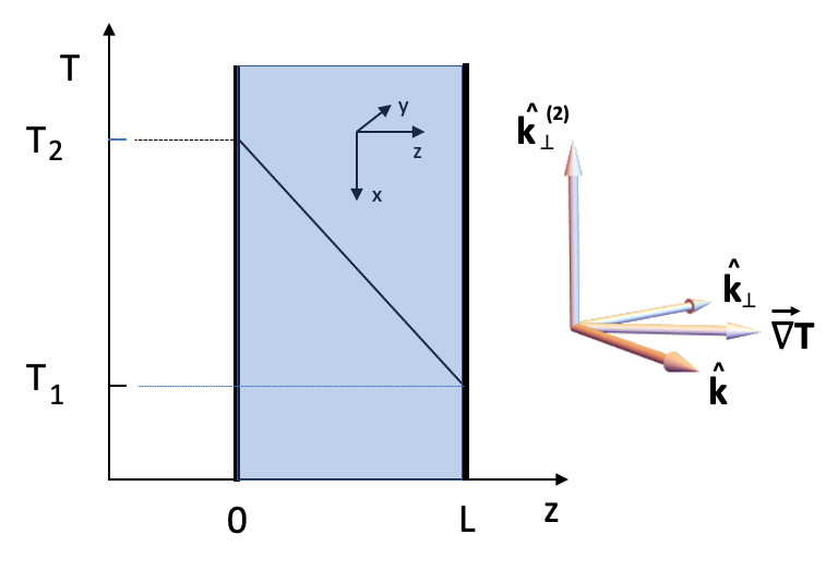
Figure 1: A fluid subject to a constant temperature gradient in the $z$-direction between two parallel confining plates. $\hat{\bm{k}}$, $\hat{\bm{k}}_{\perp}$, and $\hat{\bm{k}}_{\perp}^{(2)}$ are unit vectors that span the wave-number space, with the coordinate system chosen such that $\hat{\bm{k}}$ and $\hat{\bm{k}}_{\perp}$ are coplanar with the temperature gradient.

Consider a fluid confined between two plates that is subject to a constant temperature gradient ${\bm{\nabla}}T$ in the $z$-direction, see Fig. 1. Let ${\bm{k}}$ be the wave vector of a temperature fluctuation, and let the wave-vector space be spanned by three mutually perpendicular unit vectors $\hat{\bm{k}}={\bm{k}}/k$, $\hat{\bm{k}}_{\perp}$, and $\hat{\bm{k}}_{\perp}^{(2)}$ such that $\hat{\bm{k}}_{\perp}$ is coplanar with ${\bm{k}}$ and ${\bm{\nabla}}T$. For our purposes the temperature gradient will appear in the combination $\nabla_{\!\perp}T\equiv\hat{\bm{k}}_{\perp}\!\cdot\!{\bm{\nabla}}T$. For definiteness, we consider a fermionic quantum fluid (e.g., conduction electrons in metals). Analogous effects must be present in bosonic fluids as well, but at asymptotically low temperatures Bose-Einstein condensation will lead to complications that require additional investigation. Let $\tau$ be the relaxation time, $v_{\text{F}}$ the Fermi velocity, and $\omega$ the frequency. We need to distinguish between the hydrodynamic regime, where $\omega<1/\tau$ or $v_{\text{F}}k<1/\tau$, and the collisionless regime where $\omega>1/\tau$. The latter is in general subdivided into regimes where ${\hbar}\,\omega<T$ and ${\hbar}\,\omega>T$, respectively, see Fig. 2 Pla . Here $T$ is the spatially averaged temperature spa .

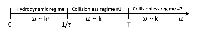
Figure 2: Frequency regimes. The hydrodynamic regime is characterized by a diffusive shear velocity, with the frequency $\omega$ scaling as the wave number squared. In the collisionless regimes the shear velocity is a propagating mode with the frequency scaling linearly with the wave number.

We are interested in the correlation functions for the temperature $T$ and the component $u_{\perp}\equiv\hat{\bm{k}}_{\perp}\cdot{\bm{u}}_{\perp}$ of the fluid shear velocity ${\bm{u}}_{\perp}$. The nature of the latter changes from diffusive to propagating as one goes from the hydrodynamic regime to the collisionless one. In the latter a hydrodynamic description no longer applies and one has to work with a quantum kinetic theory. In what follows we first state our results and then comment on their derivations. For details see the Supplemental Material SM_ .

Hydrodynamic Regime: In the hydrodynamic regime one has $\omega<1/\tau<T/\hbar$ Pla , and the correlation functions are the same as in a classical fluid. In particular, $S_{AB}^{\text{sym}}$ becomes a classical correlation function $\langle A\,B\rangle$ with the angular brackets denoting a classical statistical mechanics average, and we have Kirkpatrick et al. [1982a]:

$$S^{\text{sym}}_{TT}({\bm{k}},\omega) = \frac{2T^{2}}{c_{V}}\,\frac{D_{\text{T}}k^{2}}{\omega^{2}+(D_{\text{T}}k^{2})^{2}}$$ (5a)

$$\hskip-40.0pt+\,(\nabla_{\!\perp}T)^{2}\,\frac{2T}{\rho}\,\frac{\nu k^{2}}{(\omega^{2}+(D_{\text{T}}k^{2})^{2})(\omega^{2}+(\nu k^{2})^{2})}\qquad$$

The first term is the standard equilibrium contribution, and the second term is the long-ranged NESS contribution. $$c_{V} \rho D_{\text{T}} \nu$$ and are the spatially averaged specific heat per volume and the fluid mass density, respectively, and and are the spatially averaged heat diffusion coefficient and kinematic viscosity, respectively. The velocity-velocity correlation function is the same as in equilibrium,

$$S^{\text{sym}}_{u_{\perp}u_{\perp}}({\bm{k}},\omega)=\frac{2T}{\rho}\,\frac{\nu k^{2}}{\omega^{2}+(\nu k^{2})^{2}}\ ,$$ (5b)

and the mixed symmetrized correlation functions are

$$S^{\text{sym}}_{u_{\perp}T}({\bm{k}},\omega) = S^{\text{sym}}_{Tu_{\perp}}(-{\bm{k}},-\omega)$$ (5c)

$$= \nabla_{\!\perp}T\,\frac{1}{\rho}\,\frac{\nu k^{2}}{\omega^{2}+(\nu k^{2})^{2}}\,\frac{2T}{i\omega+D_{\text{T}}k^{2}}\ .\$$

The corresponding commutator correlation functions are given by Eq. (2) with $$\hbar\coth(\hbar\,\omega/2T)\approx 2T/\omega$$:

$$\chi^{\prime\prime}_{AB}({\bm{k}},\omega)=S^{\text{sym}}_{AB}({\bm{k}},\omega)\,\omega/2T\qquad(A,B=T,u_{\perp})\ .$$ (5d)

The static correlation functions are

$$S^{\text{sym}}_{TT}({\bm{k}}) = \frac{T^{2}}{c_{V}}+\frac{T(\nabla_{\!\perp}T)^{2}}{\rho D_{\text{T}}(\nu+D_{\text{T}})\,k^{4}}\ ,$$ (6a)

$$S^{\text{sym}}_{u_{\perp}u_{\perp}}({\bm{k}}) = T/\rho\ ,$$ (6b)

$$S^{\text{sym}}_{u_{\perp}T}({\bm{k}}) = S^{\text{sym}}_{Tu_{\perp}}(-{\bm{k}})=\nabla_{\!\perp}T\,\frac{T/\rho}{(\nu+D_{\text{T}})k^{2}}\ ,$$ (6c)

and

$$\chi_{AB}({\bm{k}})=S^{\text{sym}}_{AB}({\bm{k}})/T\qquad(A,B=T,u_{\perp})\ .$$ (6d)

$S^{\text{sym}}_{TT}({\bm{k}})$ in Eq. (6a) is the equal-time temperature-temperature correlation function mentioned in the introduction that diverges as $1/k^{4}$. This result is exactly the same as for a classical fluid, as expected in the hydrodynamic regime.

Collisionless Regime: In the collisionless regime the expressions for the dynamic correlation functions are lengthy and are given in the Supplemental Material, together with an outline of their derivations SM_ . Here we give only the results for the static temperature-temperature correlations. To leading order as $T\to 0$ we have

$$\chi_{TT}({\bm{k}})=\frac{1}{N_{\text{F}}}\,\frac{3}{\pi^{2}}\left[1+\frac{\pi^{2}}{12}\,(2\pi^{2}-3)\,\frac{(\nabla_{\!\perp}T)^{2}}{\epsilon_{\text{F}}^{2}k^{2}}\right]\$$ (7)

everywhere in the collisionless regime. Here $N_{\text{F}}$ is the density of states at the Fermi level, and $\epsilon_{\text{F}}$ is the Fermi energy. The symmetrized correlation function is $S^{\text{sym}}_{TT}({\bm{k}})=T\chi_{TT}({\bm{k}})$ in Collisionless Regime #1 in Fig. 2 and, apart from a factor of $O(1)$, $S^{\text{sym}}_{TT}({\bm{k}})\approx v_{\text{F}}k\,\chi_{TT}({\bm{k}})$ in Collisionless Regime #2.

To derive these results we note that in the hydrodynamic regime the usual Navier-Stokes equations are applicable, as they are based on very general physical principles, viz., the conservation laws for mass, momentum, and energy combined with force-balance considerations Landau and Lifshitz [1966], Chaikin and Lubensky [1995], us_ . Consequently, they hold for quantum fluids as well as for classical ones. In order to calculate correlation functions, they need to be augmented by fluctuating forces Landau and Lifshitz [1966], Kirkpatrick and Belitz [2022]. Of the various nonlinearities we need to keep only the crucial coupling between the temperature fluctuation and the transverse velocity, which turns into a linear term in the presence of a fixed temperature gradient. We can further ignore pressure fluctuations, which lead to sound waves (or plasmons in a charged Fermi liquid) that are much faster than the diffusive shear fluctuations. The equations for the operator-valued temperature and shear velocity then are

$$\left(-i\omega+\nu{\bm{k}}^{2}\right){\hat{u}}_{\perp}({\bm{k}},\omega)={\hat{P}}_{\perp}({\bm{k}},\omega)\ ,\qquad\quad$$ (8a)

$$\left(-i\omega+D_{T}{\bm{k}}^{2}\right){\hat{T}}({\bm{k}},\omega)+(\nabla_{\!\perp}T){\hat{u}}_{\perp}({\bm{k}},\omega)={\hat{Q}}({\bm{k}},\omega)\ .$$ (8b)

Here the transport coefficients $\nu$ and $D_{\text{T}}$ are to be understood as having been spatially averaged. ${\hat{P}}_{\perp}$ and $\hat{Q}$ are operator-valued fluctuating forces that are Gaussian distributed with zero mean. Their second moments can be obtained from the somewhat more general expressions derived in Ref. Kirkpatrick and Belitz [2022] and are given explicitly in the Supplemental Material SM_ . The $u_{\perp}$-$u_{\perp}$ correlation then is determined by the $P_{\perp}$ correlation and given by Eq. (5b). This is the same as in equilibrium since the temperature does not couple into the $u_{\perp}$ equation. The equilibrium part of the $T$-$T$ correlation is given by the $Q$ correlation, whereas the non-equilibrium part, as well as the mixed $T$-$u_{\perp}$ correlation, is given in terms of the $u_{\perp}$ fluctuation, with $\nabla_{\!\perp}T$ serving as a coupling constant. This yields the second term in Eq. (5a), and Eq. (5c). The leading singularity in the static $T$-$T$ correlation function is $1/k^{4}$, and $1/k^{2}$ in the $T$-$u_{\perp}$ correlation function, as in a classical fluid. This is because the hydrodynamic equations are the same in either case.

In order to properly describe the collisionless regime one has to work with the fluctuating quantum kinetic theory developed in Ref. Kirkpatrick and Belitz [2022], see the Supplemental Material for a derivation SM_ . However, the qualitative features of the results can be obtained from simple scaling arguments as follows. In the collisionless regime the diffusive inverse propagators of the form ${\cal D}^{-1}({\bm{k}},\omega)=\omega+iDk^{2}$ that appear on the left-hand sides of Eqs. (8), where $D$ can represent either $\nu$ or $D_{\text{T}}$, effectively turn into propagating zero modes of the form $\omega\mp ck$, with $c\approx v_{\text{F}}$ the propagation speed. The transport coefficients thus effectively become singular functions of the wave number and scale as $D\sim v_{\text{F}}/k$. The low-temperature result for $\chi_{TT}$, Eq. (7), then follows from Eq. (6a) by replacing $\nu,D_{\text{T}}\to v_{\text{F}}/k$ and using the low-temperature expression for the specific heat, $c_{V}\propto N_{\text{F}}T$ (prefactors, as well as issues regarding reality and signs, require a more detailed analysis). For the symmetrized correlation function one needs to consider the frequency integral in Eq. (3a) and recognize that for the equilibrium contribution it needs to be cut off at $\omega\approx D_{\text{T}}k^{2}$. In the limits $D_{\text{T}}k^{2}\ll T{/\hbar}$ and $D_{\text{T}}k^{2}\gg T{/\hbar}$, and using again the effective scaling of $D_{\text{T}}$ and $\nu$ explained above, one then obtains the relations between $S^{\text{sym}}_{TT}({\bm{k}})$ and $\chi_{TT}({\bm{k}})$ given after Eq. (7).

As mentioned above, the commutator functions $\chi^{\prime\prime}$ do not determine the linear response of the NESS to external perturbations, in contrast to an equilibrium system. In order to determine the response functions we consider the averaged Navier-Stokes equations in the presence of a field $h_{u_{\perp}}$ conjugate to $u_{\perp}$:

$$\left(-i\omega+\nu k^{2}\right)u_{\perp}({\bm{k}},\omega) = \frac{\nu}{\rho}\,k^{2}h_{u_{\perp}}({\bm{k}},\omega)\ ,$$ (9a)

$$\left(-i\omega+D_{T}k^{2}\right)\delta T({\bm{k}},\omega) + (\nabla_{\!\perp}T)u_{\perp}({\bm{k}},\omega)=$$ (9b)

$$\hskip-20.0pt\frac{1}{\rho}(\nabla_{\!\perp}T)h_{u_{\perp}}({\bm{k}},\omega)\ .\qquad$$

To avoid misunderstandings, we stress that these are equations for averaged, classical fluctuations $\delta T$ and $u_{\perp}$. They are the standard Navier-Stokes equations Landau and Lifshitz [1966] except that the sound modes have been omitted since they occur on time scales much faster than the diffusive shear and temperature fluctuations. They are driven by an external field $h_{u_{\perp}}$ that essentially represents a shift of the velocity reference frame and can be regarded as a field conjugate to $u_{\perp}$ Hohenberg and Halperin [1977], Chaikin and Lubensky [1995]. It can be experimentally realized by imposing a shear velocity on the system. For a derivation from kinetic theory, see Ref. Kirkpatrick and Belitz, 2023. The response functions $X_{AB}({\bm{k}},\omega)$ are defined by

$$u_{\perp}({\bm{k}},\omega) = X_{u_{\perp}u_{\perp}}({\bm{k}},\omega)\,h_{u_{\perp}}({\bm{k}},\omega)\ .$$ (10a)

$$\delta T({\bm{k}},\omega) = X_{Tu_{\perp}}({\bm{k}},\omega)\,h_{u_{\perp}}({\bm{k}},\omega)\ ,$$ (10b)

From Eqs. (9) we find

$$X_{u_{\perp}u_{\perp}}({\bm{k}},\omega) = \frac{1}{\rho}\,\frac{\nu k^{2}}{-i\omega+\nu k^{2}}\ .$$ (11a)

$$X_{Tu_{\perp}}({\bm{k}},\omega) = \frac{1}{\rho}\,(\nabla_{\!\perp}T)\,\frac{1}{-i\omega+D_{\text{T}}k^{2}}\,\frac{-i\omega}{-i\omega+\nu k^{2}}\ .$$

(11b)

From Eqs. (5b) and (11a) we see that the spectrum sem of $X_{u_{\perp}u_{\perp}}$, $X^{\prime\prime}_{u_{\perp}u_{\perp}}({\bm{k}},\omega)=\text{Im}\,X_{u_{\perp}u_{\perp}}({\bm{k}},\omega)$, equals the commutator correlation function $\chi^{\prime\prime}({\bm{k}},\omega)$, as expected. However, the spectrum of $X_{Tu_{\perp}}$,

$$X_{Tu_{\perp}}^{\prime\prime}({\bm{k}},\omega)=-(\nabla_{\!\perp}T)\,\frac{\omega(\nu D_{\text{T}}k^{2}-\omega^{2})}{(\omega^{2}+D_{\text{T}}^{2}k^{4})(\omega^{2}+\nu^{2}k^{4})}\ ,$$ (12)

while showing the same scaling behavior as $\chi^{\prime\prime}_{Tu_{\perp}}$, see Eqs. (5c, 5d), is not identical with the latter. In particular, the static response function vanishes,

$$X_{Tu_{\perp}}({\bm{k}})=\int\frac{d\omega}{\pi}\,\frac{X_{Tu_{\perp}}^{\prime\prime}({\bm{k}},\omega)}{\omega}=0\ ,$$ (13)

while the static correlation function is nonzero, see Eq. (6c). Nonetheless, the response functions still provide a way to directly measure the commutator correlation functions, without relying on their symmetrized counterparts that are suppressed at low temperatures. Specifically, considering Eqs. (10), (11), and (5c, 5d) we have

$$\delta T({\bm{k}},\omega)\,u_{\perp}(-{\bm{k}},-\omega)=\frac{i}{\rho}\,\chi^{\prime\prime}_{Tu_{\perp}}({\bm{k}},\omega)\,|h_{u_{\perp}}({\bm{k}},\omega)|^{2}$$ (14)

That is, the commutator $T$-$u_{\perp}$ correlation function describes the bilinear response of the product of the temperature and the shear velocity to the field conjugate to $u_{\perp}$. Similarly, the non-equilibrium part of the commutator $T$-$T$ correlation function can be expressed as a bilinear response to the field $h_{u_{\perp}}$. We define an observable

$${\tilde{T}}({\bm{k}},\omega)=T({\bm{k}},\omega)-\frac{1}{\rho}\,(\nabla_{\!\perp}T)\,\frac{1}{-i\omega+D_{\text{T}}k^{2}}\,h_{u_{\perp}}({\bm{k}},\omega)$$ (15)

that obeys the equation

$$\left(-i\omega+D_{T}k^{2}\right)\delta{\tilde{T}}({\bm{k}},\omega)+(\nabla_{\!\perp}T)u_{\perp}({\bm{k}},\omega)=0\ .$$ (16)

The physical interpretation of Eq. (16) is the heat equation with a streaming term that contains the absolute shear velocity, whereas Eq. (9b) contains the shear velocity relative to the field $h_{u_{\perp}}$. The response of ${\tilde{T}}$ to the field $h_{u_{\perp}}$ is given by a response function

$$X_{{\tilde{T}}u_{\perp}}({\bm{k}},\omega)=\frac{1}{\rho}\,(\nabla_{\!\perp}T)\,\frac{-1}{-i\omega+D_{\text{T}}k^{2}}\,\frac{\nu k^{2}}{-i\omega+\nu k^{2}}\ .$$ (17)

From Eqs. (17), (11b), (5a), and (5d) we find that the non-equilibrium part of the commutator $T$-$T$ correlation function describes the bilinear response of the product of $\tilde{T}$ and $T$ to the field $h_{u_{\perp}}$:

$$\delta{\tilde{T}}({\bm{k}},\omega)\,\delta T(-{\bm{k}},-\omega)=\frac{i}{\rho}\,\chi_{TT}^{\prime\prime\text{\,neq}}({\bm{k}},\omega)\,|h_{u_{\perp}}({\bm{k}},\omega)|^{2}$$ (18)

The Eqs. (14) and (18) constitute our main result. They demonstrate that in a NESS characterized by a constant temperature gradient the commutator correlation functions for the temperature and the shear velocity are still related to the response of the system to an external shear perturbation, even though the usual fluctuation-dissipation theorem is not valid. In contrast to the situation in equilibrium, where the correlation functions are the same as the response functions, in a NESS the correlation functions are given by the bilinear response of products of observables. We note that Eqs. (14) and (18) involve the non-equilibrium parts of the correlation functions only. For $\Delta T\to 0$, $\chi^{\prime\prime}_{Tu_{\perp}}$ vanishes and $\chi^{\prime\prime}_{TT}$ reduces to its equilibrium part that obeys the usual fluctuation-dissipation theorem.

To summarize, we have established a relation between correlation functions and response functions for a fluid in a NESS. The resulting NESS fluctuation formulas (14) and (18) resemble the equilibrium fluctuation-dissipation theorem, Eq. (2) in the hydrodynamic limit, with the symmetrized correlation function replaced by the product of two averaged observables, and the temperature replaced by the driving field squared. The driving field, which is realized by an imposed shear velocity, one has experimental control over regardless of how low the temperature is. We stress that we have derived this relation between the fluctuation functions and the response functions only for the special case of a constant temperature gradient. Their structure suggests that they might hold for more general nonequilibrium states as well, but whether or not that is true is an open question. We also have determined the quantum analogs of the long-ranged correlations known to exist in a classical fluid in a NESS. In the latter context we note that in a fermionic quantum fluid there potentially (depending on the values of the Landau Fermi-liquid parameters) are many other zero modes that also display $\omega\sim k$ scaling, in addition to the shear velocity. These can change the prefactor of the singularity, but not the scaling behavior. Also, in a charged Fermi liquid (e.g., conduction electrons in metals) the first-sound mode turns into the massive plasmon, so our approximation of neglecting pressure fluctuations is valid a fortiori.

For the purpose of this Supplemental Material section we use units such that $\hbar=k_{\text{B}}=1$.

Fluctuating-Force Correlations

For the explicit determination of correlation functions one needs the correlations of the fluctuating forces ${\hat{P}}_{\perp}$ and ${\hat{Q}}$ in Eqs. (8). They follow from the correlations of a more general Langevin operator that were determined in Ref. Kirkpatrick and Belitz, 2022. ${\hat{Q}}$ is related to the fluctuating heat current denoted by $\hat{\bm{q}}_{\text{L}}$ in that reference by

$$c_{p}\,{\hat{Q}}({\bm{k}},\omega)=-i{\bm{k}}\cdot{\hat{\bm{q}}}_{\text{L}}({\bm{k}},\omega)\ ,$$ (S0)

where $c_{p}$ is the specific heat at constant pressure, and ${\hat{P}}_{\perp}$ is related to the fluctuating stress tensor ${\hat{\tau}}_{\text{L}}$ in the same reference by

$${\hat{P}}_{\perp}({\bm{k}},\omega)=\frac{-i}{\rho}\,{\hat{k}}_{\perp}^{i}k^{j}({\hat{\tau}}_{\text{L}})_{ij}({\bm{k}},\omega)\ .$$ (S0)

The force correlations are obtained from Eqs. (3.24) in Ref. Kirkpatrick and Belitz, 2022. One obtains

$$\frac{1}{2}\left\langle\left[{\hat{Q}}({\bm{k}}_{1},\omega_{1}),{\hat{Q}}({\bm{k}}_{2},\omega_{2})\right]_{\pm}\right\rangle=2\pi\delta(\omega_{1}+\omega_{2})\,V\delta_{{\bm{k}}_{1},-{\bm{k}}_{2}}\,\frac{D_{T}}{c_{p}}\,{\bm{k}}_{1}^{2}\,\omega_{1}Tc_{\pm}(\omega_{1}/2T)\ ,$$ (S0)

$$\frac{1}{2}\left\langle\left[{\hat{P}}_{\perp}({\bm{k}}_{1},\omega_{1}),{\hat{P}}_{\perp}({\bm{k}}_{2},\omega_{2})\right]_{\pm}\right\rangle=-2\pi\delta(\omega_{1}+\omega_{2})\,V\delta_{{\bm{k}}_{1},-{\bm{k}}_{2}}\,\frac{\nu}{\rho}\,k_{1}^{2}\,\omega_{1}c_{\pm}(\omega_{1}/2T)\ ,$$ (S0)

where

$$c_{\pm}(\Omega)=\begin{cases}1&\text{for}\quad+\\ \coth\Omega&\text{for}\quad-\end{cases}$$ (S0)

The cross correlations vanish,

$$\left\langle\left[{\hat{Q}}({\bm{k}}_{1},\omega_{1}),{\hat{P}}_{\perp}({\bm{k}}_{2},\omega_{2})\right]_{\pm}\right\rangle=0\ .$$ (S0)

With Eqs. (S3) - (S6) the correlation functions in the hydrodynamic regime, Eqs. (5), (6) in the main text, are easily determined.

Correlation Functions in the Collisionless Regime

Kinetic Theory

For the correlation functions in the collisionless regime one needs to utlilize kinetic theory. Let

$$f_{\bm{p}}^{\text{eq}}=\frac{1}{e^{(\epsilon_{p}-\mu)/T}+1}$$ (S0)

be the equilibrium Fermi-Dirac distribution, with $\epsilon_{p}$ the single-particle energy and $\mu$ the chemical potential, and let ${\hat{f}}({\bm{p}},{\bm{x}},t)$ be the operator-valued single-particle distribution function which, in the collisionless regime, is governed by a fluctuating Boltzmann-Landau kinetic equation Lifshitz and Pitaevskii [1981], Kirkpatrick and Belitz [2022]

$$\partial_{t}{\hat{f}}({\bm{p}},{\bm{x}},t)+{\bm{v}}_{\bm{p}}\cdot{\bm{\nabla}}_{\bm{x}}{\hat{f}}({\bm{p}},{\bm{x}},t)=w({\bm{p}})\,{\hat{F}}_{\text{L}}({\bm{p}},{\bm{x}},t)\ .$$ (S0)

Here

$$w({\bm{p}})=-\partial f_{\bm{p}}^{\text{eq}}/\partial\epsilon_{p}=\frac{1}{4T\cosh^{2}((\epsilon_{p}-\mu)/2T)}\ ,$$ (S0)

and ${\hat{F}}_{\text{L}}$ is a fluctuating-force operator whose correlations were given in Sec. II.C of Ref. Kirkpatrick and Belitz, 2022. Now consider the local equilibrium distribution

$$f_{\bm{p}}^{(0)}({\bm{x}},t)=\frac{1}{\exp\left[\left(\frac{({\bm{p}}-m{\bm{u}}({\bm{x}},t))^{2}}{2m}-\mu({\bm{x}},t)\right)/T({\bm{x}},t)\right]+1}\ ,$$ (S0)

with ${\bm{u}}$, $\mu$, and $T$ the local fluid velocity, chemical potential, and temperature, respectively Chapman and Cowling [1970], and write

$${\hat{f}}({\bm{p}},{\bm{x}},t)=f_{\bm{p}}^{(0)}({\bm{x}},t)+w({\bm{p}})\,{\hat{\phi}}({\bm{p}},{\bm{x}},t)\ .$$ (S0)

In the presence of an externally imposed temperature gradient ${\bm{\nabla}}T$ the streaming term in Eq. (S8) acting on the local equilibrium distribution produces a term proportional to ${\bm{\nabla}}T$. We neglect pressure fluctuations as we did in the hydrodynamic regime, and keep only the crucial coupling of ${\bm{\nabla}}T$ to the shear velocity, ignoring all other effects of the temperature gradient. It is convenient to define functions

$$a_{5}({\bm{p}})=\epsilon_{p}-\mu+T(\partial\mu/\partial T)_{N,V}$$ (S0)

and

$$a_{s}({\bm{p}})=a_{5}({\bm{p}})-(T/n)(\partial p/\partial T)_{N,V}=\epsilon_{p}-\mu-sT/n$$ (S0)

with $s/n$ the averaged entropy per particle. Then we obtain for the linearized version of Eq. (S8)

$$\left(\partial_{t}+{\bm{v}}_{\bm{p}}\cdot{\bm{\nabla}}_{\bm{x}}\right){\hat{\phi}}({\bm{p}},{\bm{x}},t)={\hat{F}}_{\text{L}}({\bm{p}},{\bm{x}},t)-{\hat{u}}_{\perp}({\bm{x}},t)\,\frac{({\hat{\bm{k}}}_{\perp}\!\!\cdot\!{\bm{\nabla}}T)}{T}\,a_{s}({\bm{p}})\ .$$ (S0)

This generalizes Eq. (2.6b) in Ref. Kirkpatrick and Belitz, 2022 to the situation of a constant temperature gradient while neglecting the Fermi-liquid interactions. Performing Fourier transforms in space and time, we now have

$${\hat{\phi}}({\bm{p}},{\bm{k}},\omega)=G_{0}({\bm{p}},{\bm{k}},\omega)\biggl{[}{\hat{F}}_{\text{L}}({\bm{p}},{\bm{k}},\omega)-\hat{u}_{\perp}({\bm{k}},\omega)\,\frac{({\hat{\bm{k}}}_{\perp}\!\!\cdot\!{\bm{\nabla}}T)}{T}\,a_{s}({\bm{p}})\biggr{]}\ ,$$ (S0)

with

$$G_{0}({\bm{p}},{\bm{k}},\omega)=\frac{i}{\omega-{\bm{k}}\cdot{\bm{p}}/m+i0}$$ (S0)

a Green function.

Correlation Functions

Temperature fluctuations are defined as linear combinations of fluctuations of the internal energy density $e$ and the number density $n$,

$$\delta T=\left(\frac{\partial T}{\partial e}\right)_{n,V}\delta e+\left(\frac{\partial T}{\partial n}\right)_{e,V}\delta n$$ (S0)

This is true classically, and it remains true if the classical fluctuations are replaced by their operator-value quantum mechanical counterparts. In terms of the function $\hat{\phi}$ this implies

$$\delta{\hat{T}}({\bm{k}},\omega)=\frac{1}{c_{V}}\,\frac{1}{V}\sum_{\bm{p}}a_{5}({\bm{p}})\,w({\bm{p}})\,{\hat{\phi}}({\bm{p}},{\bm{k}},\omega)\ .$$ (S0)

Substituting (S0) this becomes

$$\delta{\hat{T}}({\bm{k}},\omega)=\frac{1}{c_{V}}\,\frac{1}{V}\sum_{\bm{p}}w({\bm{p}})\,a_{5}({\bm{p}})\,G_{0}({\bm{p}},{\bm{k}},\omega)\,{\hat{F}}_{\text{L}}({\bm{p}},{\bm{k}},\omega)-({\hat{\bm{k}}}_{\perp}\!\!\cdot\!{\bm{\nabla}}T)\,{\hat{u}}_{\perp}({\bm{k}},\omega)\,\tau({\bm{k}},\omega)\ ,$$ (S0)

where

$$\tau({\bm{k}},\omega)=\frac{1}{c_{V}T}\,\frac{1}{V}\sum_{\bm{p}}w({\bm{p}})\,a_{5}({\bm{p}})\,a_{s}({\bm{p}})\,G_{0}({\bm{p}},{\bm{k}},\omega)\ .$$ (S0)

In the low-temperature limit this becomes

$$\tau({\bm{k}},\omega)=\frac{N_{\text{F}}T}{c_{V}}\,\frac{\pi^{2}}{6}\,\frac{-i}{v_{\text{F}}k}\,\log\left(\frac{1-\omega/v_{\text{F}}k-i0}{-1-\omega/v_{\text{F}}k-i0}\right)+O(T^{3})\ .$$ (S0)

We see that the equilibrium part of the temperature fluctuations is given by the fluctuating force, whereas the non-equilibrium part is given by the fluctuations of the shear velocity. The latter are given by

$${\hat{u}}_{\perp}({\bm{k}},\omega)=\frac{1}{\rho}\,\frac{1}{V}\sum_{\bm{p}}({\hat{\bm{k}}}_{\perp}\cdot{\bm{p}})\,w({\bm{p}})\,{\hat{\phi}}({\bm{p}},{\bm{k}},\omega)\ .$$ (S0)

Using (S0) again, and the fluctuating force correlations from Ref. Kirkpatrick and Belitz, 2022, we find, to leading order as $T\to 0$,

$$\frac{1}{2}\Big{\langle}\left[{\hat{u}}_{\perp}({\bm{k}}_{1},\omega_{1}),{\hat{u}}_{\perp}({\bm{k}}_{2},\omega_{2})\right]_{\pm}\Big{\rangle}=2\pi\delta(\omega_{1}+\omega_{2})\,V\,\delta_{{\bm{k}}_{1},-{\bm{k}}_{2}}\,\frac{\pi}{\rho^{2}}\,\omega_{1}\,\frac{1}{V}\sum_{\bm{p}}w({\bm{p}})\,\left(\hat{\bm{k}}_{1\perp}\cdot{\bm{p}}\right)^{2}\delta(\omega_{1}-{\bm{k}}_{1}\cdot{\bm{p}}/m)\,c_{\pm}(\omega_{1}/2T)$$ (S0)

with $c_{\pm}$ from (S5). Here we have used the expressions for the fluctuating-force correlations given in Ref. Kirkpatrick and Belitz, 2022, in particular (2.11), (2.18), (2.15c), and (3.7) in that paper.

We can now assemble the temperature-temperature correlation functions. We find

$$\chi^{\prime\prime}_{TT}({\bm{k}},\omega)=\frac{\pi}{c_{V}^{2}}\,\frac{1}{V}\sum_{\bm{p}}w({\bm{p}})\,\left(a_{5}({\bm{p}})\right)^{2}\omega\,\delta(\omega-{\bm{k}}\cdot{\bm{p}}/m)\hskip 220.0pt\mbox{}$$

$$\qquad+\,\omega\,\frac{\pi}{4}\,\frac{(\nabla_{\!\perp}T)^{2}}{v_{\text{F}}^{2}k^{2}}\,\frac{k_{\text{F}}^{2}}{\rho^{2}}\,\frac{1}{V}\sum_{\bm{p}}w({\bm{p}})\left(1-(\hat{\bm{k}}\cdot\hat{\bm{p}})^{2}\right)\left[\log^{2}\left|\frac{1-\hat{\bm{k}}\cdot\hat{\bm{p}}}{1+\hat{\bm{k}}\cdot\hat{\bm{p}}}\right|+\pi^{2}\right]\,\delta(\omega-{\bm{k}}\cdot{\bm{p}}/m)$$ (S0)

and

$$S^{\text{sym}}_{TT}({\bm{k}},\omega)=\chi^{\prime\prime}_{TT}({\bm{k}},\omega)\,\coth(\omega/2T)$$ (S0)

From these expressions one can determine the static correlation functions. At $T=0$, $w({\bm{p}})$ turns into a delta function and for $\chi_{TT}({\bm{k}})$ one obtains obtains Eq. (7) in the main text.

References

- Nyquist [1928] H. Nyquist. Thermal agitation of electric charge in conductors. Phys. Rev., 32:110, 1928.
- Callen and Welton [1951] H. B. Callen and T. A. Welton. Irreversibility and generalized noise. Phys. Rev., 83:34, 1951.
- Forster [1975] D. Forster. Hydrodynamic Fluctuations, Broken Symmetry, and Correlation Functions. Benjamin, Reading, MA, 1975.
- Sevick et al. [2008] E. M. Sevick, R. Prabhakar, S. R. Williams, and D. J. Searles. Fluctuation theorems. Annu. Rev. Phys. Chem., 59:603, 2008.
- Gaspard [2022] P. Gaspard. The Statistical Mechanics of Irreversible Phenomena. Cambridge University Press, Cambridge, UK, 2022.
- Baiesi and Maes [2013] M. Baiesi and C. Maes. An update on the nonequilibrium linear response. New J. Phys., 15:103004, 2013.
- Andrieux and Gaspard [2004] D. Andrieux and P. Gaspard. Fluctuation theorem and Onsager reciprocity relations. J. Chem. Phys., 121:6167, 2004.
- Maes [2020] C. Maes. Frenesy: time-symmetric dynamical activity in nonequilibria. Phys. Rep., 805:1, 2020.
- Kirkpatrick et al. [1982a] T. R. Kirkpatrick, E. G. D. Cohen, and J. R. Dorfman. Light scattering by a fluid in a nonequilibrium steady state. II. Large gradients. Phys. Rev. A, 26:995, 1982a.
- Dorfman et al. [1994] J. R. Dorfman, T. R. Kirkpatrick, and J. V. Sengers. Generic long-range correlations in molecular fluids. Ann. Rev. Phys. Chem., 45:213, 1994.
- Ortiz de Zárate and Sengers [2007] J. M. Ortiz de Zárate and J. V. Sengers. Hydrodynamic fluctuations in fluids and fluid mixtures. Elsevier, Amsterdam, 2007.
- Kirkpatrick et al. [1982b] T. R. Kirkpatrick, E. G. D. Cohen, and J. R. Dorfman. Fluctuations in a nonequilibrium steady state: Basic equations. Phys. Rev. A, 26:950, 1982b.
- Ronis and Procaccia [1982] D. Ronis and I. Procaccia. Nonlinear resonant coupling between shear and heat fluctuations in fluids far from equilibrium. Phys. Rev. A, 26:1812, 1982.
- Sengers et al. [2016] J. V. Sengers, J. M. Ortiz de Zárate, and T. R. Kirkpatrick. Thermal fluctuations in non-equilibrium steady states. In D. Bedeaux, S. Kjelstrup, and J. V. Sengers, editors, Non-equilibrium thermodynamics with applications, chapter 3, page 39. RSC Publishing, Cambridge, 2016.
- Anderson [1984] P. W. Anderson. Basic Notions of Condensed Matter Physics. Benjamin, Menlo Park, CA, 1984.
- Kirkpatrick et al. [2021] T. R. Kirkpatrick, D. Belitz, and J. R. Dorfman. Superfast signal propagation in fluids and solids in non-equilibrium steady states. J. Chem. Phys. B, 125:7499, 2021.
- [17] Our approach to quantum fluids Kirkpatrick and Belitz [2022] is based on a quantum mechanical version of the classical hydrodynamic equations for collective variables Landau and Lifshitz [1966], Pines and Nozières [1989]. It should not be confused with the hydrodynamic formulation of quantum mechanics that has received much interest over almost 100 years, see, e.g., Refs. Wyatt, 2005, Ruggiero et al., 2020 and references therein.
- [18] Note that the commutator correlations still exist in the classical limit, due to the factor of in the definition. Alternatively, they can be defined in terms of Poisson brackets.
- [19] In an ordinary Fermi liquid, , with the Fermi energy. More generally, can scale with a smaller power of , but always holds Hartnoll and Mackenzie [2022].
- [20] The spatial average is taken over the entire system. This approximation neglects effects of the temperature gradient that are less leading than the one caused by the term in Eq. (5b) Kirkpatrick et al. [1982a].
- [21] See the Supplemental Material section below.
- Landau and Lifshitz [1966] L. D. Landau and E. M. Lifshitz. Fluid Mechanics, chapter XVII. Pergamon, Oxford, Third Revised English edition, 1966. Many editions are missing this chapter.
- Chaikin and Lubensky [1995] P. Chaikin and T. C. Lubensky. Principles of Condensed Matter Physics. Cambridge University, Cambridge, 1995.
- [24] For a derivation of the linearized Navier-Stokes equations from quantum kinetic theory, see Ref. Kirkpatrick and Belitz, 2022.
- Kirkpatrick and Belitz [2022] T. R. Kirkpatrick and D. Belitz. Fluctuating quantum kinetic theory. Phys. Rev. B, 105:245147, 2022.
- Hohenberg and Halperin [1977] P. C. Hohenberg and B. I. Halperin. Theory of dynamic critical phenomena. Rev. Mod. Phys., 49:435, 1977.
- Kirkpatrick and Belitz [2023] T. R. Kirkpatrick and D. Belitz. Velocity-dependent forces and non-hydrodynamic initial conditions in quantum and classical fluids. arXiv:2304.06157, 2023.
- [28] Some authors, e.g., Pines and Noziéres Pines and Nozières [1989], refer to as the ‘spectral density’ of .
- Pines and Nozières [1989] D. Pines and P. Nozières. The Theory of Quantum Liquids. Addison-Wesley, Redwood City, CA, 1989.
- Wyatt [2005] R. E. Wyatt. Quantum Dynamics with Trajectories: Introduction to Quantum Hydrodynamics. Springer, NY, 2005.
- Ruggiero et al. [2020] P. Ruggiero, P. Calabrese, B. Doyon, and J. Dubail. Quantum generalized hydrodynamics. Phys. Rev. Lett., 124:140603, 2020.
- Hartnoll and Mackenzie [2022] S. A. Hartnoll and A. P. Mackenzie. Planckian dissipation in metals. Rev. Mod. Phys., 94:041002, 2022.
SUPPLEMENTAL MATERIAL

References

- Kirkpatrick and Belitz [2022] T. R. Kirkpatrick and D. Belitz. Fluctuating quantum kinetic theory. Phys. Rev. B, 105:245147, 2022.
- Lifshitz and Pitaevskii [1981] E. M. Lifshitz and L. P. Pitaevskii. Statistical Physics, Part 2. Pergamon, Oxford, second edition, 1981.
- Chapman and Cowling [1970] S. Chapman and T. G. Cowling. The Mathematical Theory of Nonuniform Gases. Cambridge University, Cambridge, 1970.