ACTC: Active Threshold Calibration
for Cold-Start Knowledge Graph Completion

Abstract

Self-supervised knowledge-graph completion (KGC) relies on estimating a scoring model over (entity, relation, entity)-tuples, for example, by embedding an initial knowledge graph. Prediction quality can be improved by calibrating the scoring model, typically by adjusting the prediction thresholds using manually annotated examples. In this paper, we attempt for the first time cold-start calibration for KGC, where no annotated examples exist initially for calibration, and only a limited number of tuples can be selected for annotation.

Our new method ACTC finds good per-relation thresholds efficiently based on a limited set of annotated tuples. Additionally to a few annotated tuples, ACTC also leverages unlabeled tuples by estimating their correctness with Logistic Regression or Gaussian Process classifiers. We also experiment with different methods for selecting candidate tuples for annotation: density-based and random selection. Experiments with five scoring models and an oracle annotator show an improvement of 7% points when using ACTC in the challenging setting with an annotation budget of only 10 tuples, and an average improvement of 4% points over different budgets.

1 Introduction

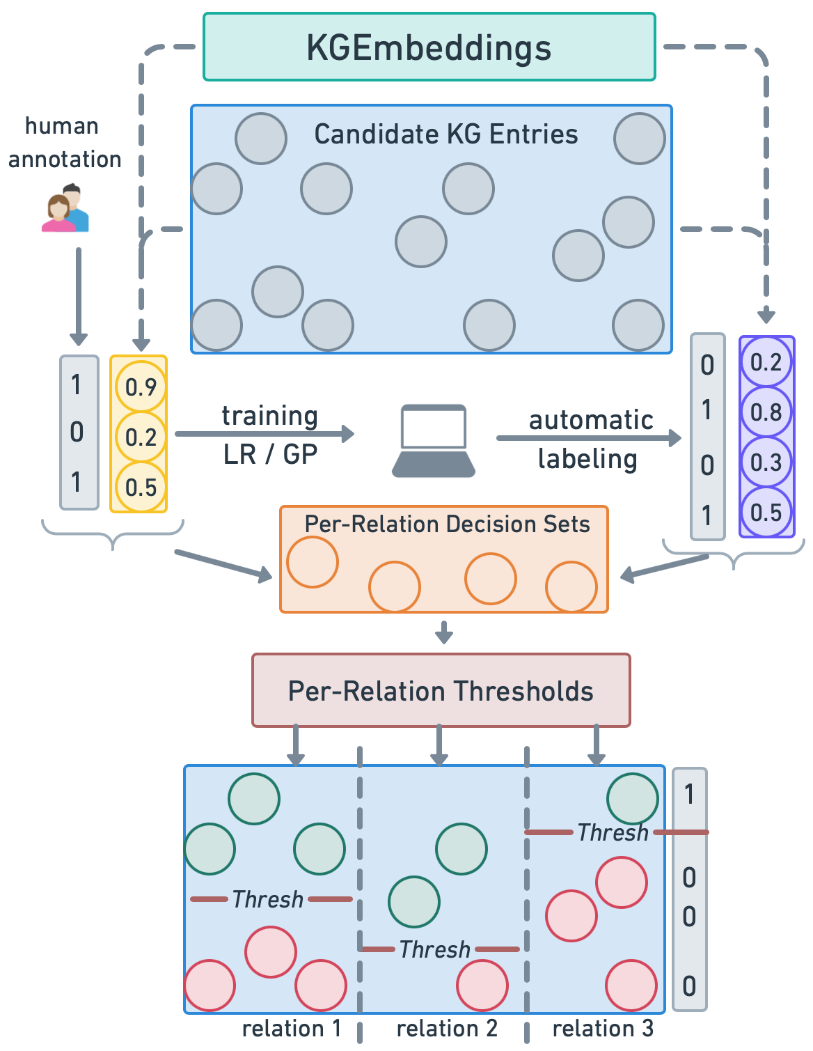
Figure 1: ACTC method. The manually annotated samples are used to train a Logistic Regression or Gaussian Processes classifier, which labels the additional tuples using their scores predicted by a KGE model. All annotations (manual and automatic) are later used to estimate the per-relation thresholds.

Knowledge graphs (KG) organize knowledge about the world as a graph where entities (nodes) are connected by different relations (edges). The knowledge-graph completion (KGC) task aims at adding new information in the form of (entity, relation, entity) triples to the knowledge graph. The main objective is assigning to each triple a plausibility score, which defines how likely this triple belongs to the underlying knowledge base. These scores are usually predicted by the knowledge graph embedding (KGE) models. However, most KGC approaches do not make any binary decision and provide a ranking, not classification, which does not allow one to use them as-is to populate the KGs Speranskaya et al. (2020). To transform the scores into predictions (i.e., how probable is it that this triple should be included in the KG), decision thresholds need to be estimated. Then, all triples with a plausibility score above the threshold are classified as positive and included in the KG; the others are predicted to be negatives and not added to the KG. Since the initial KG includes only positive samples and thus cannot be used for threshold calibration, the calibration is usually performed on a manually annotated set of positive and negative tuples (decision set). However, manual annotation is costly and limited, and, as most knowledge bases include dozens Ellis et al. (2018), hundreds Toutanova and Chen (2015) or even thousands Auer et al. (2007) of different relation types, obtaining a sufficient amount of labeled samples for each relation may be challenging. This raises a question:

How to efficiently solve the cold-start thresholds calibration problem with minimal human input?

We propose a new method for Active Threshold Calibration ACTC, which estimates the relation thresholds by leveraging unlabeled data additionally to human-annotated data. In contrast to already existing methods Safavi and Koutra (2020); Speranskaya et al. (2020) that use only the annotated samples, ACTC labels additional samples automatically with a trained predictor (Logistic Regression or Gaussian Process model) estimated on the KGE model scores and available annotations. A graphical illustration of ACTC is provided in Figure 1.

Our main contributions are:

• We are the first to study threshold tuning in a budget-constrained environment. This setting is more realistic and challenging in contrast to the previous works where large validation sets have been used for threshold estimation.

• We propose actively selecting examples for manual annotation, which is also a novel approach for the KGC setting.

• We leverage the unlabeled data to have more labels at a low cost without increasing the annotation budget, which is also a novel approach for the KGC setting.

Experiments on several datasets and with different KGE models demonstrate the efficiency of ACTC for different amounts of available annotated samples, even for as little as one.

2 Related Work

Knowledge graph embedding methods Dettmers et al. (2017); Trouillon et al. (2016); Bordes et al. (2013); Nickel et al. (2011) have been originally evaluated on ranking metrics, not on the actual task of triple classification, which would be necessary for KGC. More recent works have acknowledged this problem by creating data sets for evaluating KGC (instead of ranking) and proposed simple algorithms for finding prediction thresholds from annotated triples Speranskaya et al. (2020); Safavi and Koutra (2020). In our work, we study the setting where only a limited amount of such annotations can be provided, experiment with different selection strategies of samples for annotation, and analyze how to use them best. Ostapuk et al. (2019) have studied active learning for selecting triples for training a scoring model for KG triples, but their method cannot perform the crucial step of calibration. They consequently only evaluate on ranking metrics, not measuring actual link prediction quality. In contrast, our approach focuses on selecting much fewer samples for optimal calibration of a scoring model (using positive, negative, and unlabeled samples).

3 ACTC: Active Threshold Calibration

ACTC consists of three parts: selection of samples for manual annotation, automatic labeling of additional samples, and estimating the per-relation thresholds based on all available labels (manual and automatic ones).

The first step is selecting unlabeled samples for human annotation. In ACTC this can be done in two ways. One option is a random sampling from the set of all candidate tuples ($\textbf{ACTC}_{rndm}$; the pseudocodes can be found in Algorithm 1). However, not all annotations are equally helpful and informative for estimation. To select the representative and informative samples that the system can profit the most from, especially with a small annotation budget, we also introduce density-based selection $\textbf{ACTC}_{dens}$ inspired by the density-based selective sampling method in active learning Agarwal et al. (2020); Zhu et al. (2008) (the pseudocode can be found in Algorithm 2 in Appendix A). The sample density is measured by summing the squared distances between this sample’s score (predicted by the KGE model) and the scores of other samples in the unlabeled dataset. The samples with the highest density are selected for human annotation.

In a constrained-budget setting with a limited amount of manual annotations available, there are sometimes only a few samples annotated for some relations and not even one for others. To mitigate this negative effect and to obtain good thresholds even with limited manual supervision, ACTC labels more samples (in addition to the manual annotations) with a classifier trained on the manually annotated samples to predict the labels based on the KGE model scores. We experiment with two classifiers: Logistic Regression (ACTC-LR) and Gaussian Processes (ACTC-GP). The amount of automatically labeled samples depends on hyper-parameter $n$, which reflects the minimal amount of samples needed for estimating each threshold (see ablation study of different n values in Section 5). If the number of samples annotated for a relation $r$ ($l_{r}$) is larger or equal to $n$, only these $l_{r}$ annotated samples are used for threshold estimation. If the amount of manually annotated samples is insufficient (i.e., less than $n$), the additional $n-l_{r}$ samples are randomly selected from the dataset and labeled by a LR or GP classifier. The automatically labeled and manually annotated samples build a per-relation threshold decision set, which contains at least $n$ samples for a relation $r$ with (manual or predicted) labels. The threshold for relation $r$ is later optimized on this decision set.

Algorithm 1 $ACTC_{rndm}$ algorithm

Input: unlabeled dataset $\mathcal{X}$, annotation budget size $l$, minimal decision set size $n$, KGE model $M$, classifier $\mathcal{C}:\mathbb{R}\to[0,1]$
Output: set of per-relation thresholds $T$

 

1:# Step 1: samples selection for human annotation

2:$T\leftarrow$ a set of per-relational thresholds

3:$\mathcal{X}_{gold}\leftarrow$ randomly selected $l$ samples from $\mathcal{X}$

4:manually annotate $\mathcal{X}_{gold}$ with $y_{gold}$ labels

5:for relation $r$ do

6:     $\mathcal{X}_{{gold}_{r}}\leftarrow$ samples from $\mathcal{X}_{gold}$ with relation $r$

7:     $y_{{gold}_{r}}\leftarrow$ manual labels for $\mathcal{X}_{{gold}_{r}}$

8:     $scores_{{gold}_{r}}\leftarrow$ KGE model scores for $\mathcal{X}_{{gold}_{r}}$

9:     $l_{r}\leftarrow|\mathcal{X}_{{gold}_{r}}|$

10:# Step 2: automatically label additional samples

11:     if $n>l_{r}$ then

12:         Train a classifier $\mathcal{C}_{r}$ on $scores_{{gold}_{r}}$ and $y_{{gold}_{r}}$

13:         $\mathcal{X}_{{auto}_{r}}\leftarrow$ rand. selected $n-l_{r}$ samples from $\mathcal{X}$

14:         $scores_{{auto}_{r}}\leftarrow$ KGE model scores for $\mathcal{X}_{{auto}_{r}}$

15:         Predict $y_{{auto}_{r}}=\mathcal{C}_{r}(scores_{{auto}_{r}})$

16:         $\mathcal{X}_{dec}=(\mathcal{X}_{{gold}_{r}},y_{{gold}_{r}})\bigcup(\mathcal{X}_{{auto}_{r}},y_{{auto}_{r}})$

17:     else

18:         $\mathcal{X}_{dec}=(\mathcal{X}_{{gold}_{r}},y_{{gold}_{r}}$)      

19:# Step 3: estimate per-relation threshold $\tau_{r}$

20:     $\tau\leftarrow 0,best\_acc\leftarrow 0$

21:     for $score$ in $scores_{{gold}_{r}}$ do

22:         $\tau_{i}\leftarrow score$

23:         $accuracy_{i}\leftarrow acc(scores_{{gold}_{r}},y_{{gold}_{r}}|\tau_{i})$

24:         if $accuracy_{i}>best\_acc$ then

25:              $\tau\leftarrow\tau_{i}$

26:              $best\_acc\leftarrow accuracy_{i}$               

27:     $T.append(\tau)$

The final part of the algorithm is the estimation of the relation-specific thresholds. Each sample score from the decision set is tried out as a potential threshold; the relation-specific thresholds that maximize the local accuracy (calculated for this decision set) are selected.

4 Experiments

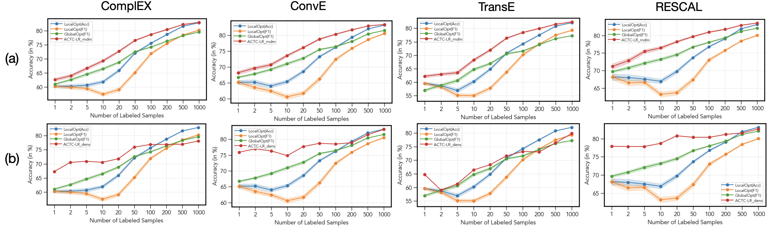
Figure 2: $ACTC-LR_{rndm}$ (upper) and $ACTC-LR_{dens}$ (lower) performance for different amounts of manually annotated samples and with different KGE models.

We evaluate our method on two KGC benchmark datasets extracted from Wikidata and augmented with manually verified negative samples: CoDEx-s and CoDEx-m Safavi and Koutra (2020). Some details on their organization are provided in Appendix B. The KGE models are trained on the training sets. The ACTC algorithm is applied on the validation sets: the gold validation labels are taken as an oracle (manual annotations; in an interactive setting they would be presented to human annotators on-the-fly); the remaining samples are used unlabeled. The test set is not exploited during ACTC training and serves solely for testing purposes. The dataset statistics are provided in Table 1. We run our experiments with four KGE models: ComplEx Trouillon et al. (2016), ConvE Dettmers et al. (2017), TransE Bordes et al. (2013), RESCAL Nickel et al. (2011). More information is provided in Appendix C.

Data	#Train	#Val	#Test	#Ent	#Rel
CoDEx-S	32,888	3,654	3,656	2,034	42
CoDEx-M	185,584	20,620	20,622	17,050	51

Table 1: Datasets statistics. The training sets contain only positive triples. The ratio of positive to negative samples in validation and test sets is 1:1.

	CoDEx-s								CoDEx-m								Avg
	ComplEx		ConvE		TransE		RESCAL		ComplEx		ConvE		TransE		RESCAL
	Acc	F1	Acc	F1	Acc	F1	Acc	F1	Acc	F1	Acc	F1	Acc	F1	Acc	F1	Acc	F1
LocalOpt (Acc)	70	70	72	72	69	68	74	73	72	70	68	66	65	64	68	67	70	69
Safavi and Koutra (2020)	$\pm 3$	$\pm 3$	$\pm 3$	$\pm 2$	$\pm 3$	$\pm 3$	$\pm 2$	$\pm 2$	$\pm 2$	$\pm 2$	$\pm 3$	$\pm 2$	$\pm 3$	$\pm 3$	$\pm 3$	$\pm 2$
LocalOpt (F1)	67	69	69	70	65	67	70	71	70	69	66	66	63	64	66	67	67	68
	$\pm 3$	$\pm 3$	$\pm 3$	$\pm 2$	$\pm 3$	$\pm 3$	$\pm 2$	$\pm 2$	$\pm 2$	$\pm 2$	$\pm 2$	$\pm 2$	$\pm 3$	$\pm 3$	$\pm 3$	$\pm 2$
GlobalOpt (F1)	70	74	74	77	68	71	76	79	73	75	68	70	65	68	68	71	70	73
Speranskaya et al. (2020)	$\pm 2$	$\pm 2$	$\pm 1$	$\pm 2$	$\pm 2$	$\pm 2$	$\pm 1$	$\pm 1$	$\pm 1$	$\pm 2$	$\pm 1$	$\pm 2$	$\pm 2$	$\pm 2$	$\pm 1$	$\pm 2$
$ACTC-LR_{dens}$	72	72	77	78	69	71	80	81	78	77	72	71	64	65	72	70	73	73
	$\pm 3$	$\pm 2$	$\pm 1$	$\pm 1$	$\pm 2$	$\pm 2$	$\pm 1$	$\pm 1$	$\pm 0$	$\pm 1$	$\pm 1$	$\pm 1$	$\pm 1$	$\pm 1$	$\pm 1$	$\pm 1$
$ACTC-GP_{dens}$	72	72	76	78	69	71	80	80	78	77	72	70	64	65	73	71	73	73
	$\pm 3$	$\pm 2$	$\pm 1$	$\pm 1$	$\pm 1$	$\pm 2$	$\pm 1$	$\pm 1$	$\pm 0$	$\pm 0$	$\pm 1$	$\pm 1$	$\pm 2$	$\pm 2$	$\pm 2$	$\pm 1$
$ACTC-LR_{rndm}$	74	74	77	77	73	72	79	79	78	78	72	72	69	69	73	73	74	74
	$\pm 3$	$\pm 2$	$\pm 2$	$\pm 2$	$\pm 3$	$\pm 3$	$\pm 1$	$\pm 1$	$\pm 1$	$\pm 1$	$\pm 2$	$\pm 2$	$\pm 3$	$\pm 2$	$\pm 2$	$\pm 2$
$ACTC-GP_{rndm}$	74	74	77	77	73	72	81	81	77	77	71	71	67	66	72	71	74	74
	$\pm 3$	$\pm 2$	$\pm 2$	$\pm 2$	$\pm 3$	$\pm 3$	$\pm 1$	$\pm 1$	$\pm 1$	$\pm 1$	$\pm 2$	$\pm 2$	$\pm 3$	$\pm 3$	$\pm 2$	$\pm 2$

Table 2: ACTC results in % averaged across different sizes of annotation budget reported with the standard error of the mean. The experiment with each annotation budget was repeated 100 times.

4.1 Baselines

ACTC is compared to three baselines. The first baseline LocalOpt (Acc) optimizes the per-relation thresholds towards the accuracy: for each relation, the threshold is selected from the embedding scores assigned to the samples with manual annotations that contain this relation, so that the local accuracy (i.e., accuracy, which is calculated only for these samples) is maximized (Safavi and Koutra, 2020). We also modified this approach into LocalOpt (F1) by changing the maximization metric to the local F1 score. The third baseline is GlobalOpt, where the thresholds are selected by iterative search over a manually defined grid Speranskaya et al. (2020). The best thresholds are selected based on the global F1 score calculated for the whole dataset. In all baselines, the samples for manual annotation are selected randomly.

4.2 Results

We ran the experiments for the following number of manually annotated samples: 1, 2, 5, 10, 20, 50, 100, 200, 500, and 1000. Experimental setup details are provided in Appendix E. Table 2 provides the result averaging all experiments (here and further, $n=500$ for a fair comparison; see Section 5 for analyze of $n$ value), and our method ACTC outperforms the baselines in every tried setting as well as on average. Figure 2a also demonstrates the improvement of $ACTC_{rndm}$ over the baselines for every tried amount of manually annotated samples on the example of CoDEx-s dataset; the exact numbers of experiments with different budgets are provided in Appendix F. The density-based selection, on the other hand, achieves considerably better results when only few manually annotated samples are available (see Figure 2b). Indeed, choosing representative samples from the highly connected clusters can be especially useful in the case of lacking annotation. $LR_{dense}$, which selects points from regions of high density, can be helpful for small annotation budgets since it selects samples that are similar to other samples. In contrast, when having a sufficient annotation budget and after selecting a certain number of samples, dense regions are already sufficiently covered, and $LR_{rndm}$ provides a more unbiased sample from the entire distribution.

5 Ablation Study

A more detailed ablation study of different ACTC settings is provided in Appendix D.

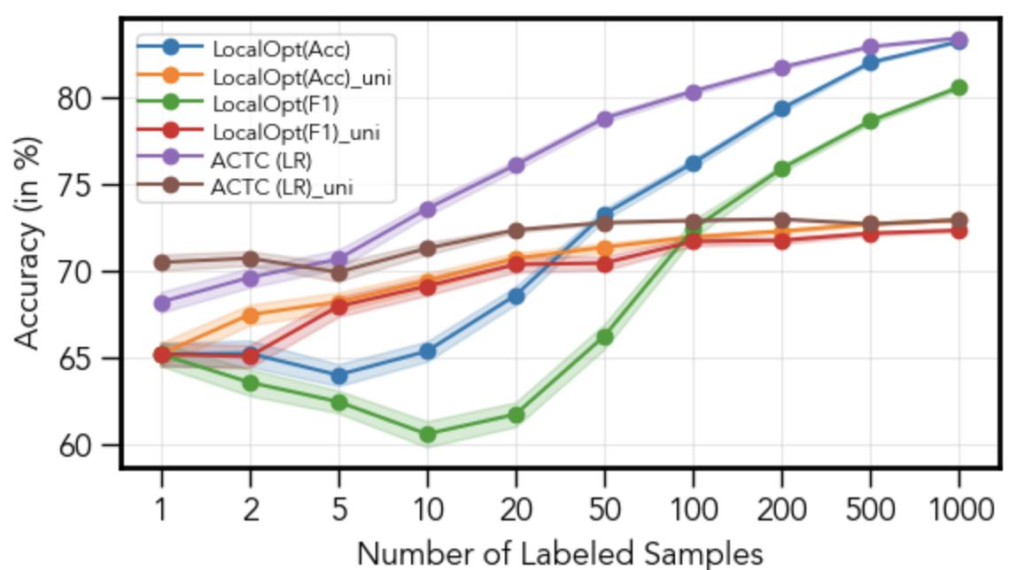
Figure 3: The universal threshold calibration methods compared to the per-relation methods.

Global Thresholds.

All methods described above calibrate the per-relation thresholds. Another option is to define a uniform (uni) threshold, which works as a generic threshold for all tuples regardless the relations involved. We implemented it as $ACTC-LR_{uni}$ method, where the additional samples are automatically labeled and used to build a decision dataset together with the manually annotated ones - in the same way as done for the relation-specific version, but only once for the whole dataset (thus, significantly reducing the computational costs). We also applied the LocalOpt(Acc) and LocalOpt(F1) baselines in the uniform setting. Figure 3 demonstrates the results obtained with the Conve KGE model and random selection mechanism on the CodEX-s dataset. Although the universal versions generally perform worse than the relation-specific, $ACTC_{uni}$ still outperforms the universal baselines and even relation-specific ones for a small annotation budget.

Different n values.

An important parameter in ACLC is n, the minimal sufficient amount of (manually or automatically) labeled samples needed to calibrate the threshold. The ablation study of different n values is provided in Figure 4 on the example of $ACTC-LR_{dens}$ setting, averaged across all annotation budgets. ACTC performs as a quite stable method towards the n values. Even a configuration with a minimum value of $n=5$ outperforms baselines with a small annotation budget or even with quite large one (e.g. for RESCAL).

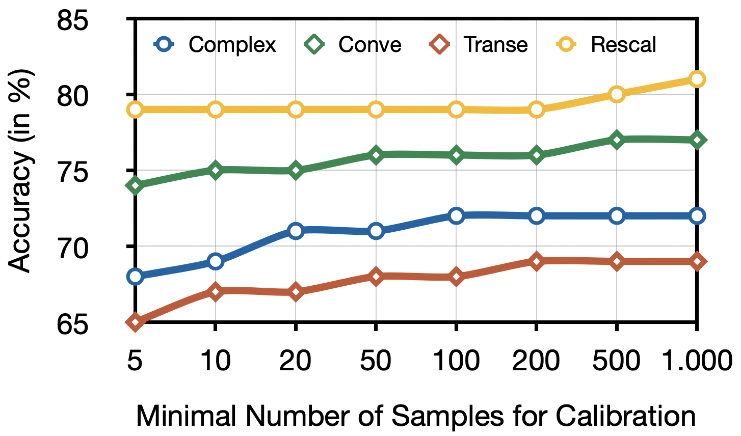
Figure 4: Ablation study for different n values.

6 Conclusion

In this work, we explored for the first time the problem of cold-start calibration of scoring models for knowledge graph completion. Our new method for active threshold calibration ACTC provides different strategies of selecting the samples for manual annotation and automatically labels additional tuples with Logistic Regression and Gaussian Processes classifiers trained on the manually annotated data. Experiments on datasets with oracle positive and negative triple annotations, and several KGE models, demonstrate the efficiency of our method and the considerable increase in the classification performance even for tiny annotation budgets.

7 Limitations

A potential limitation of our experiments is the use of oracle validation labels instead of human manual annotation as in the real-world setting. However, all validation sets we used in our experiments were collected based on the manually defined seed set of entities and relations, carefully cleaned and augmented with manually labeled negative samples. Moreover, we chose this more easy-to-implement setting to make our results easily reproducible and comparable with future work.

Another limitation of experiments that use established data sets and focus on isolated aspects of knowledge-graph construction is their detachment from the real-world scenarios. Indeed, in reality knowledge graph completion is done in a much more complicated environment, that involves a variety of stakeholders and aspects, such as data verification, requirements consideration, user management and so on. Nevertheless, we do believe that our method, even if studied initially in isolation, can be useful as one component in real world knowledge graph construction.

8 Ethics Statement

Generally, the knowledge graphs used in the experiments are biased towards the North American cultural background, and so are evaluations and predictions made on them. As a consequence, the testing that we conducted in our experiments might not reflect the completion performance for other cultural backgrounds. Due to the high costs of additional oracle annotation, we could not conduct our analysis on more diverse knowledge graphs. However, we have used the most established and benchmark dataset with calibration annotations, CoDEx, which has been collected with significant human supervision. That gives us hope that our results will be as reliable and trustworthy as possible.

While our method can lead to better and more helpful predictions from knowledge graphs, we cannot guarantee that these predictions are perfect and can be trusted as the sole basis for decision-making, especially in life-critical applications (e.g. healthcare).

Appendix A $\textbf{ACTC}_{dens}$ Pseudocode

	CoDEx-s								CoDEx-m								Avg
	ComplEx		ConvE		TransE		RESCAL		ComplEx		ConvE		TransE		RESCAL
	Acc	F1	Acc	F1	Acc	F1	Acc	F1	Acc	F1	Acc	F1	Acc	F1	Acc	F1	Acc	F1
LocalOpt (Acc)	70	70	72	72	69	68	74	73	72	70	68	66	65	64	68	67	70	69
Safavi and Koutra (2020)	$\pm 3$	$\pm 3$	$\pm 3$	$\pm 2$	$\pm 3$	$\pm 3$	$\pm 2$	$\pm 2$	$\pm 2$	$\pm 2$	$\pm 3$	$\pm 2$	$\pm 3$	$\pm 3$	$\pm 3$	$\pm 2$
LocalOpt (F1)	67	69	69	70	65	67	70	71	70	69	66	66	63	64	66	67	67	68
	$\pm 3$	$\pm 3$	$\pm 3$	$\pm 2$	$\pm 3$	$\pm 3$	$\pm 2$	$\pm 2$	$\pm 2$	$\pm 2$	$\pm 2$	$\pm 2$	$\pm 3$	$\pm 3$	$\pm 3$	$\pm 2$
GlobalOpt (F1)	70	74	74	77	68	71	76	79	73	75	68	70	65	68	68	71	70	73
Speranskaya et al. (2020)	$\pm 2$	$\pm 2$	$\pm 1$	$\pm 2$	$\pm 2$	$\pm 2$	$\pm 1$	$\pm 1$	$\pm 1$	$\pm 2$	$\pm 1$	$\pm 2$	$\pm 2$	$\pm 2$	$\pm 1$	$\pm 2$
$ACTC-LR_{dens}$	72	72	77	78	69	71	80	81	78	77	72	71	64	65	72	70	73	73
	$\pm 3$	$\pm 2$	$\pm 1$	$\pm 1$	$\pm 2$	$\pm 0$	$\pm 1$	$\pm 1$	$\pm 0$	$\pm 1$	$\pm 1$	$\pm 1$	$\pm 1$	$\pm 1$	$\pm 1$	$\pm 1$
$ACTC-GP_{dens}$	72	72	76	78	69	71	80	80	78	77	72	70	64	65	73	71	73	73
	$\pm 3$	$\pm 2$	$\pm 1$	$\pm 1$	$\pm 1$	$\pm 2$	$\pm 1$	$\pm 1$	$\pm 0$	$\pm 0$	$\pm 1$	$\pm 1$	$\pm 2$	$\pm 2$	$\pm 2$	$\pm 1$
$ACTC-LR_{rndm}$	74	74	77	77	73	72	79	79	78	78	72	72	69	69	73	73	74	74
	$\pm 3$	$\pm 2$	$\pm 2$	$\pm 2$	$\pm 3$	$\pm 3$	$\pm 1$	$\pm 1$	$\pm 1$	$\pm 1$	$\pm 2$	$\pm 2$	$\pm 3$	$\pm 2$	$\pm 2$	$\pm 2$
$ACTC-GP_{rndm}$	74	74	77	77	73	72	81	81	77	77	71	71	67	66	72	71	74	74
	$\pm 3$	$\pm 2$	$\pm 2$	$\pm 2$	$\pm 3$	$\pm 3$	$\pm 1$	$\pm 1$	$\pm 1$	$\pm 1$	$\pm 2$	$\pm 2$	$\pm 3$	$\pm 3$	$\pm 2$	$\pm 2$
$ACTC-LR_{dens}(F1)$	72	72	73	75	63	66	78	79	78	77	72	72	64	66	72	71	72	73
	$\pm 3$	$\pm 2$	$\pm 0$	$\pm 0$	$\pm 0$	$\pm 1$	$\pm 0$	$\pm 1$	$\pm 1$	$\pm 1$	$\pm 1$	$\pm 2$	$\pm 2$	$\pm 1$	$\pm 3$	$\pm 2$
$ACTC-GP_{dens}(F1)$	72	73	76	78	68	70	79	80	78	77	71	71	64	66	71	73	72	74
	$\pm 2$	$\pm 1$	$\pm 1$	$\pm 1$	$\pm 1$	$\pm 2$	$\pm 1$	$\pm 1$	$\pm 1$	$\pm 2$	$\pm 2$	$\pm 1$	$\pm 1$	$\pm 1$	$\pm 1$	$\pm 3$
$ACTC-LR_{rndm}(F1)$	73	74	77	78	72	74	79	80	76	75	69	70	66	67	70	70	73	74
	$\pm 3$	$\pm 2$	$\pm 2$	$\pm 1$	$\pm 3$	$\pm 2$	$\pm 1$	$\pm 1$	$\pm 2$	$\pm 1$	$\pm 2$	$\pm 2$	$\pm 3$	$\pm 2$	$\pm 2$	$\pm 2$
$ACTC-GP_{rndm}(F1)$	74	74	77	77	72	73	79	79	77	77	70	71	67	68	71	72	73	74
	$\pm 1$	$\pm 2$	$\pm 2$	$\pm 2$	$\pm 3$	$\pm 2$	$\pm 1$	$\pm 1$	$\pm 3$	$\pm 2$	$\pm 1$	$\pm 2$	$\pm 1$	$\pm 3$	$\pm 1$	$\pm 1$

Table 3: ACTC results in % averaged across different size of annotation budget reported with the standard error of the mean. The ACTC method is provided in two local optimization setting: first, the thresholds maximize accuracy (in the same way as it was presented in Figure 2), second, the thresholds are maximized towards F1 score. The experiment with each annotation budget was repeated 100 times.

Algorithm 2 $ACTC_{dens}$ algorithm

Input: unlabeled dataset $\mathcal{X}$, annotation budget size $l$, minimal decision set size $n$, KGE model $M$, classifier $\mathcal{C}:\mathbb{R}\to[0,1]$
Output: set of per-relation thresholds $T$

 

1:# Step 1: samples selection for human annotation

2:$T\leftarrow$ a set of per-relational thresholds

3:for $i=0,1,...,|\mathcal{X}|$ do

4:     $density_{x_{i}}=\sum_{j=0}^{|\mathcal{X}|}(score_{j}-score_{i})^{2}$

5:$\mathcal{X}_{gold}\leftarrow$ top $l$ samples with maximal $density_{x_{i}}$

6:manually annotate $\mathcal{X}_{gold}$ with $y_{gold}$ labels

7:[the rest is the same as in $ACTC_{rndm}$, see Alg. 1]

8:# Step 2: automatically label additional samples

9:[same as Step 2 in $ACTC_{rndm}$, see Alg. 1]

10:# Step 3: estimate per-relation threshold $\tau_{r}$

11:[same as Step 3 in $ACTC_{rndm}$, see Alg. 1]

Appendix B CoDEx datasets

In our experiments, we use benchmark CoDEx datasets Safavi and Koutra (2020). The datasets were collected based on the Wikidata in the following way: a seed set of entities and relations for 13 domains (medicine, science, sport, etc) was defined and used as queries to Wikidata in order to retrieve the entities, relations, and triples. After additional postprocessing (e.g. removal of inverse relations), the retrieved data was used to construct 3 datasets: CoDEx-S, CoDEx-M, and CoDEx-L. For the first two datasets, the authors additionally constructed hard negative samples (by annotating manually the candidate triples which were generated using a pre-trained embedding model), which allows us to use them in our experiments.

• An example of positive triple: (Senegal, part of, West Africa).

• An example of negative triple: (Senegal, part of, Middle East).

Appendix C Embedding models

We use four knowledge graph embedding models. This section highlights their main properties and provides their scoring functions.

ComplEX

Trouillon et al. (2016) uses complex-numbered embeddings and diagonal relation embedding matrix to score triples; the scoring function is defined as $s(h,r,t)=\mathbf{e}_{\mathbf{h}}^{T}\operatorname{diag}\left(\mathbf{r}_{\mathbf{r}}\right)\mathbf{e}_{\mathbf{t}}$.

ConvE

Dettmers et al. (2017) represents a neural approach to KGE scoring and exploits the non-linearities: $s(h,r,t)=f(\operatorname{vec}(f([\mathbf{e_{h}};\overline{\mathbf{r}}]*\omega)(\mathbf{W})\mathbf{t}$.

TransE

Bordes et al. (2013) is an example of translation KGE models, where the relations are tackled as translations between entities; the embeddings are scored with $s(h,r,t)=-\left\|\mathbf{e}_{\mathbf{h}}+\mathbf{r}_{\mathbf{r}}-\mathbf{e}_{\mathbf{t}}\right\|_{p}$.

RESCAL

Nickel et al. (2011) treats the entities as vectors and relation types as matrices and scores entities and relation embeddings with the following scoring function: $s(h,r,t)=\mathbf{e}_{\mathbf{h}}^{T}\mathbf{R}_{\mathbf{r}}\mathbf{e}_{\mathbf{t}}$.

These models were selected, first, following the previous works Safavi and Koutra (2020); Speranskaya et al. (2020), and, second, to demonstrate the performance of our method using the different KGE approaches: linear (ComplEX and RESCAL), translational (TransE), and neural (ConvE).

Appendix D Ablation Study

Optimization towards F1 score.

Just as we converted the LocalOpt (Acc) baseline from Safavi and Koutra (2020) to a LocalOpt(F1) setting, we also converted ACTC into ACTC(F1). The only difference is the metric, which the thresholds maximize: instead of accuracy, the threshold that provides the best F1 scores are looked for. Table 3 is an extended result table, which provides the ACTC(F1) numbers together with the standard ACTC (optimizing towards accuracy) and baselines. As can be seen, there is no dramatic change in ACTC performance; naturally enough, the F1 test score for ACTC(F1) experiments is slightly better than the F1 test score for experiments where thresholds were selected based on accuracy value.

	CoDEx-s								CoDEx-m								Avg
	ComplEx		ConvE		TransE		RESCAL		ComplEx		ConvE		TransE		RESCAL
	Acc	F1	Acc	F1	Acc	F1	Acc	F1	Acc	F1	Acc	F1	Acc	F1	Acc	F1	Acc	F1
LocalOpt (Acc)1	60	58	65	65	60	57	68	66	66	63	61	59	55	50	62	58	62	60
Safavi and Koutra (2020)	$\pm 1$	$\pm 2$	$\pm 1$	$\pm 1$	$\pm 1$	$\pm 1$	$\pm 1$	$\pm 2$	$\pm 1$	$\pm 2$	$\pm 1$	$\pm 1$	$\pm 0$	$\pm 2$	$\pm 1$	$\pm 2$
LocalOpt (F1)1	60	58	65	65	60	57	68	66	66	63	61	59	55	50	62	58	62	60
	$\pm 1$	$\pm 2$	$\pm 1$	$\pm 1$	$\pm 1$	$\pm 1$	$\pm 1$	$\pm 2$	$\pm 1$	$\pm 2$	$\pm 1$	$\pm 1$	$\pm 0$	$\pm 2$	$\pm 1$	$\pm 2$
GlobalOpt (F1)1	61	67	67	72	57	65	70	75	65	72	60	66	55	62	61	67	62	68
Speranskaya et al. (2020)	$\pm 0$	(1.0)	$\pm 0$	$\pm 0$	$\pm 0$	$\pm 1$	$\pm 0$	$\pm 0$	$\pm 1$	$\pm 0$	$\pm 0$	$\pm 0$	$\pm 0$	(1.0)	$\pm 0$	$\pm 0$
$ACTC-LR_{dens}^{1}$	67	68	76	77	65	66	78	79	71	75	69	66	57	65	68	62	69	70
	$\pm 0$	$\pm 0$	$\pm 0$	$\pm 0$	$\pm 0$	$\pm 0$	$\pm 0$	$\pm 0$	$\pm 0$	$\pm 0$	$\pm 0$	$\pm 0$	$\pm 0$	$\pm 0$	$\pm 0$	$\pm 0$
$ACTC-GP_{dens}^{1}$	59	47	72	76	61	59	50	67	76	76	71	70	58	66	68	62	64	65
	$\pm 0$	$\pm 0$	$\pm 0$	$\pm 0$	$\pm 1$	$\pm 1$	$\pm 0$	$\pm 0$	$\pm 0$	$\pm 0$	$\pm 0$	$\pm 0$	$\pm 0$	$\pm 0$	$\pm 0$	$\pm 0$
$ACTC-LR_{rndm}^{1}$	63	60	70	69	61	58	76	75	69	67	63	62	57	52	63	60	67	63
	$\pm 0$	$\pm 1$	$\pm 1$	$\pm 1$	$\pm 1$	$\pm 1$	$\pm 1$	$\pm 1$	$\pm 0$	$\pm 2$	$\pm 0$	$\pm 1$	$\pm 0$	$\pm 2$	$\pm 0$	$\pm 1$
$ACTC-GP_{rndm}^{1}$	63	61	71	70	61	59	76	76	74	73	64	65	56	64	65	64	66	67
	$\pm 1$	$\pm 1$	$\pm 0$	$\pm 1$	$\pm 1$	$\pm 1$	$\pm 1$	$\pm 1$	$\pm 0$	$\pm 0$	$\pm 0$	$\pm 0$	$\pm 0$	(0.02)	$\pm 0$	$\pm 0$

Table 4: ACTC results for $l=1$, $n=500$, averaged across 100 tries for each experiment and reported with the standard error of the mean

Estimate All Samples

Apart from the automatic labeling of additional samples discussed in Section 3 (i.e., the additional samples are labeled in case of insufficient manual annotations so that the size of the decision set built from manually annotated and automatically labeled samples equals $n$), we also experimented with annotating all samples. All samples that were not manually labeled are automatically labeled with a classifier. However, the performance was slightly better only for the middle budgets (i.e., for the settings with 5, 10, and 20 manually annotated samples) and became considerably worse for large budgets (i.e., 100, 200, etc), especially in the denstity_selection setting. Based on that, we can conclude that a lot of (automatically) labeled additional data is not what the model profits the most; the redundant labels (which are also not gold and potentially contain mistakes) only amplify the errors and lead to worse algorithm performance.

Hard VS Soft Labels.

The classifier’s predictions can be either directly used as real-valued soft labels or transformed to the hard ones by selecting the class with the maximum probability. In most of our experiments, the performance of soft and hard labels was practically indistinguishable (yet with a slight advantage of the latter). All the results provided in this paper were obtained with hard automatic labels.

Appendix E Experimental Setting

As no validation data is available in our setting, the ACTC method does not require any hyperparameter tuning. We did not use a GPU for our experiments; one ACTC run takes, on average, 2 minutes. All results are reproducible with a seed value $12345$.

	CoDEx-s								CoDEx-m								Avg
	ComplEx		ConvE		TransE		RESCAL		ComplEx		ConvE		TransE		RESCAL
	Acc	F1	Acc	F1	Acc	F1	Acc	F1	Acc	F1	Acc	F1	Acc	F1	Acc	F1	Acc	F1
LocalOpt (Acc)10	62	62	65	64	60	59	67	66	67	65	63	59	57	57	63	60	63	62
Safavi and Koutra (2020)	$\pm 1$	$\pm 1$	$\pm 1$	$\pm 1$	$\pm 1$	$\pm 1$	$\pm 1$	$\pm 1$	$\pm 1$	$\pm 1$	$\pm 1$	$\pm 1$	$\pm 0$	$\pm 1$	$\pm 1$	$\pm 1$
LocalOpt (F1)10	57	61	61	62	55	59	63	64	65	63	60	60	55	58	60	60	60	61
	$\pm 1$	$\pm 1$	$\pm 1$	$\pm 1$	$\pm 1$	$\pm 1$	$\pm 1$	$\pm 1$	$\pm 1$	$\pm 1$	$\pm 1$	$\pm 1$	$\pm 1$	$\pm 1$	$\pm 1$	$\pm 1$
GlobalOpt (F1)10	66	71	71	74	65	67	73	76	70	73	65	68	61	66	64	68	67	70
Speranskaya et al. (2020)	$\pm 0$	$\pm 0$	$\pm 0$	$\pm 1$	$\pm 1$	$\pm 1$	$\pm 0$	$\pm 0$	$\pm 0$	$\pm 0$	$\pm 0$	$\pm 0$	$\pm 0$	$\pm 1$	$\pm 0$	$\pm 0$
$ACTC-LR_{dens}^{10}$	70	73	74	76	66	67	79	80	77	77	71	70	61	61	73	72	71	72
	$\pm 0$	$\pm 0$	$\pm 0$	$\pm 0$	$\pm 0$	$\pm 0$	$\pm 0$	$\pm 0$	$\pm 0$	$\pm 0$	$\pm 0$	$\pm 0$	$\pm 0$	$\pm 0$	$\pm 0$	$\pm 0$
$ACTC-GP_{dens}^{10}$	64	71	73	76	68	65	78	80	77	77	72	70	61	61	73	72	71	72
	$\pm 0$	$\pm 0$	$\pm 0$	$\pm 0$	$\pm 1$	$\pm 1$	$\pm 0$	$\pm 0$	$\pm 0$	$\pm 0$	$\pm 0$	$\pm 0$	$\pm 0$	$\pm 0$	$\pm 0$	$\pm 0$
$ACTC-LR_{rndm}^{10}$	70	70	74	73	68	66	77	77	74	73	67	66	62	62	67	66	70	70
	$\pm 0$	$\pm 1$	$\pm 0$	$\pm 1$	$\pm 0$	$\pm 1$	$\pm 0$	$\pm 1$	$\pm 0$	$\pm 1$	$\pm 0$	$\pm 1$	$\pm 0$	$\pm 1$	$\pm 0$	$\pm 1$
$ACTC-GP_{rndm}^{10}$	71	70	73	73	68	65	77	77	75	74	68	67	62	61	68	67	70	70
	$\pm 0$	$\pm 1$	$\pm 0$	$\pm 1$	$\pm 1$	$\pm 1$	$\pm 0$	$\pm 1$	$\pm 0$	$\pm 1$	$\pm 0$	$\pm 1$	$\pm 1$	$\pm 1$	$\pm 1$	$\pm 1$

Table 5: ACTC results for $l=10$, $n=500$, averaged across 100 tries for each experiment and reported with the standard error of the mean

	CoDEx-s								CoDEx-m								Avg
	ComplEx		ConvE		TransE		RESCAL		ComplEx		ConvE		TransE		RESCAL
	Acc	F1	Acc	F1	Acc	F1	Acc	F1	Acc	F1	Acc	F1	Acc	F1	Acc	F1	Acc	F1
LocalOpt (Acc)50	72	73	73	74	71	71	74	74	73	72	70	69	67	68	71	70	71	71
Safavi and Koutra (2020)	$\pm 0$	$\pm 0$	$\pm 0$	$\pm 0$	$\pm 0$	$\pm 0$	$\pm 0$	$\pm 0$	$\pm 0$	$\pm 0$	$\pm 0$	$\pm 0$	$\pm 0$	$\pm 0$	$\pm 0$	$\pm 0$
LocalOpt (F1)50	65	69	66	70	64	68	67	71	69	71	66	68	64	67	67	69	66	69
	$\pm 1$	$\pm 0$	$\pm 1$	$\pm 0$	$\pm 1$	$\pm 0$	$\pm 1$	$\pm 0$	$\pm 0$	$\pm 0$	$\pm 0$	$\pm 0$	$\pm 0$	$\pm 0$	$\pm 0$	$\pm 0$
GlobalOpt (F1)50	73	76	75	78	71	73	77	79	74	76	70	72	67	71	69	72	72	75
Speranskaya et al. (2020)	$\pm 0$	$\pm 0$	$\pm 0$	$\pm 0$	$\pm 0$	$\pm 0$	$\pm 0$	$\pm 0$	$\pm 0$	$\pm 0$	$\pm 0$	$\pm 0$	$\pm 0$	$\pm 0$	$\pm 0$	$\pm 0$
$ACTC-LR_{dens}^{50}$	76	76	78	79	72	72	80	81	79	79	72	72	63	64	73	73	74	75
	$\pm 0$	$\pm 0$	$\pm 0$	$\pm 0$	$\pm 0$	$\pm 0$	$\pm 0$	$\pm 0$	$\pm 0$	$\pm 0$	$\pm 0$	$\pm 0$	$\pm 0$	$\pm 0$	$\pm 0$	$\pm 0$
$ACTC-GP_{dens}^{50}$	75	78	78	80	77	78	77	78	79	78	72	72	64	64	74	74	75	75
	$\pm 0$	$\pm 0$	$\pm 0$	$\pm 0$	$\pm 0$	$\pm 0$	$\pm 0$	$\pm 0$	$\pm 0$	$\pm 0$	$\pm 0$	$\pm 0$	$\pm 0$	$\pm 0$	$\pm 0$	$\pm 0$
$ACTC-LR_{rndm}^{10}$	76	78	79	79	76	77	80	80	78	78	71	71	69	70	73	73	75	76
	$\pm 0$	$\pm 0$	$\pm 0$	$\pm 0$	$\pm 0$	$\pm 0$	$\pm 0$	$\pm 0$	$\pm 0$	$\pm 0$	$\pm 0$	$\pm 0$	$\pm 0$	$\pm 0$	$\pm 0$	$\pm 0$
$ACTC-GP_{rndm}^{10}$	75	78	79	80	77	78	80	80	78	78	72	71	69	70	73	74	75	76
	$\pm 0$	$\pm 0$	$\pm 0$	$\pm 0$	$\pm 0$	$\pm 0$	$\pm 0$	$\pm 0$	$\pm 0$	$\pm 0$	$\pm 0$	$\pm 0$	$\pm 0$	$\pm 0$	$\pm 0$	$\pm 0$

Table 6: ACTC results for $l=50$, $n=500$, averaged across 100 tries for each experiment and reported with the standard error of the mean

ACTC does not imply any restrictions on the classifier architecture. We experimented with two classifiers: Logistic Regression classifier and Gaussian Processes classifier. For both of them, we used a Scikit-learn implementation Pedregosa et al. (2011). The Logistic Regression classifier was used in the default Scikit-learn setting, with L2 penalty term and inverse of regularization strength equals 100. In the Gaussian Processes classifier, we experimented with the following kernels:

• squared exponential RBF kernel with $length\_scale=10$

• its generalized and smoothed version, Matérn kernel, with $length\_scale=0.1$

• a mixture of different RBF kernels, RationalQuadratic kernel, with $length\_scale=0.1$

All the results for Gaussian Processes classifier provided in this paper are obtained with the Matérn kernel Minasny and McBratney (2005) using the following kernel function:

$$k\left(x_{i},x_{j}\right)=\frac{1}{\Gamma(\nu)2^{\nu-1}}\left(\frac{\sqrt{2\nu}}{l}d\left(x_{i},x_{j}\right)\right)^{\nu}*$$

$$*K_{\nu}\left(\frac{\sqrt{2\nu}}{l}d\left(x_{i},x_{j}\right)\right)$$

where $K_{\nu}$ is a Bessel function and $\Gamma$ is a Gamma function.

Appendix F Results for Different Annotation Budgets

Tables 4, 5, and 6 demonstrate the performance of the different ACTC settings for different annotation budgets (1, 10, and 50, respectively). The results are averaged over all settings; each setting was repeated 100 times. Table 4 demonstrates how useful and profitable the density-selection methods are in a lower budget setting. However, the non-biased random selection works better with more manually annotated samples (e.g., 50).

References

- Agarwal et al. (2020) Sharat Agarwal, Himanshu Arora, Saket Anand, and Chetan Arora. 2020. Contextual diversity for active learning. In Computer Vision – ECCV 2020, pages 137–153, Cham. Springer International Publishing.
- Auer et al. (2007) Sören Auer, Christian Bizer, Georgi Kobilarov, Jens Lehmann, Richard Cyganiak, and Zachary Ives. 2007. Dbpedia: A nucleus for a web of open data. In The Semantic Web, pages 722–735, Berlin, Heidelberg. Springer Berlin Heidelberg.
- Bordes et al. (2013) Antoine Bordes, Nicolas Usunier, Alberto Garcia-Duran, Jason Weston, and Oksana Yakhnenko. 2013. Translating embeddings for modeling multi-relational data. In Advances in Neural Information Processing Systems, volume 26. Curran Associates, Inc.
- Dettmers et al. (2017) Tim Dettmers, Pasquale Minervini, Pontus Stenetorp, and Sebastian Riedel. 2017. Convolutional 2d knowledge graph embeddings. CoRR, abs/1707.01476.
- Ellis et al. (2018) Joe Ellis, Jeremy Getman, and Stephanie Strassel. 2018. TAC KBP English Entity Linking - Comprehensive Training and Evaluation Data 2009-2013.
- Minasny and McBratney (2005) Budiman Minasny and Alex. B. McBratney. 2005. The matérn function as a general model for soil variograms. Geoderma, 128(3):192–207. Pedometrics 2003.
- Nickel et al. (2011) Maximilian Nickel, Volker Tresp, and Hans-Peter Kriegel. 2011. A three-way model for collective learning on multi-relational data. In Proceedings of the 28th International Conference on International Conference on Machine Learning, ICML’11, page 809–816, Madison, WI, USA. Omnipress.
- Ostapuk et al. (2019) Natalia Ostapuk, Jie Yang, and Philippe Cudre-Mauroux. 2019. Activelink: Deep active learning for link prediction in knowledge graphs. In The World Wide Web Conference, WWW ’19, page 1398–1408, New York, NY, USA. Association for Computing Machinery.
- Pedregosa et al. (2011) Fabian Pedregosa, Gaël Varoquaux, Alexandre Gramfort, Vincent Michel, Bertrand Thirion, Olivier Grisel, Mathieu Blondel, Peter Prettenhofer, Ron Weiss, Vincent Dubourg, et al. 2011. Scikit-learn: Machine learning in python. Journal of machine learning research, 12(Oct):2825–2830.
- Safavi and Koutra (2020) Tara Safavi and Danai Koutra. 2020. CoDEx: A Comprehensive Knowledge Graph Completion Benchmark. In Proceedings of the 2020 Conference on Empirical Methods in Natural Language Processing (EMNLP), pages 8328–8350, Online. Association for Computational Linguistics.
- Speranskaya et al. (2020) Marina Speranskaya, Martin Schmitt, and Benjamin Roth. 2020. Ranking vs. classifying: Measuring knowledge base completion quality. In Conference on Automated Knowledge Base Construction, AKBC 2020, Virtual, June 22-24, 2020.
- Toutanova and Chen (2015) Kristina Toutanova and Danqi Chen. 2015. Observed versus latent features for knowledge base and text inference. In Proceedings of the 3rd Workshop on Continuous Vector Space Models and their Compositionality, pages 57–66, Beijing, China. Association for Computational Linguistics.
- Trouillon et al. (2016) Théo Trouillon, Johannes Welbl, Sebastian Riedel, Eric Gaussier, and Guillaume Bouchard. 2016. Complex embeddings for simple link prediction. In Proceedings of The 33rd International Conference on Machine Learning, volume 48 of Proceedings of Machine Learning Research, pages 2071–2080, New York, New York, USA. PMLR.
- Zhu et al. (2008) Jingbo Zhu, Huizhen Wang, Tianshun Yao, and Benjamin K Tsou. 2008. Active learning with sampling by uncertainty and density for word sense disambiguation and text classification. In Proceedings of the 22nd International Conference on Computational Linguistics (Coling 2008), pages 1137–1144, Manchester, UK. Coling 2008 Organizing Committee.