X-Shooting ULLYSES: massive stars at low metallicity

Observations of individual massive stars, super-luminous supernovae, gamma-ray bursts, and gravitational-wave events involving spectacular black-hole mergers, indicate that the low-metallicity Universe is fundamentally different from our own Galaxy. Many transient phenomena will remain enigmatic until we achieve a firm understanding of the physics and evolution of massive stars at low metallicity ($Z$). The Hubble Space Telescope has devoted 500 orbits to observe $\sim$250 massive stars at low $Z$ in the ultraviolet (UV) with the COS and STIS spectrographs under the ULLYSES program. The complementary “X-Shooting ULLYSES” (XShootU) project provides enhanced legacy value with high-quality optical and near-infrared spectra obtained with the wide-wavelength coverage X-shooter spectrograph at ESO’s Very Large Telescope. We present an overview of the XShootU project, showing that combining ULLYSES UV and XShootU optical spectra is critical for the uniform determination of stellar parameters such as effective temperature, surface gravity, luminosity, and abundances, as well as wind properties such as mass-loss rates in function of $Z$. As uncertainties in stellar and wind parameters percolate into many adjacent areas of Astrophysics, the data and modelling of the XShootU project is expected to be a game-changer for our physical understanding of massive stars at low $Z$. To be able to confidently interpret James Webb Space Telescope (JWST) spectra of the first stellar generations, the individual spectra of low $Z$ stars need to be understood, which is exactly where XShootU can deliver.

1 Introduction

We find ourselves amidst a scientific revolution: gravitational wave (GW) observatories will soon be detecting black hole (BH) mergers as frequently as once per day. To interpret these events, we need to comprehend massive stars in low metallicity ($Z$) environments (Abbott et al. 2020). This is also crucial for other fields of Astrophysics, including feedback processes (e.g., Doran et al. 2013), star formation, interstellar medium (ISM) physics, supernovae (SNe), and cosmology. To enable progress in these research areas, we need to uniformly sample the relevant parameter space for massive OB stars, including spectral type, luminosity class, and metallicity ($Z$).

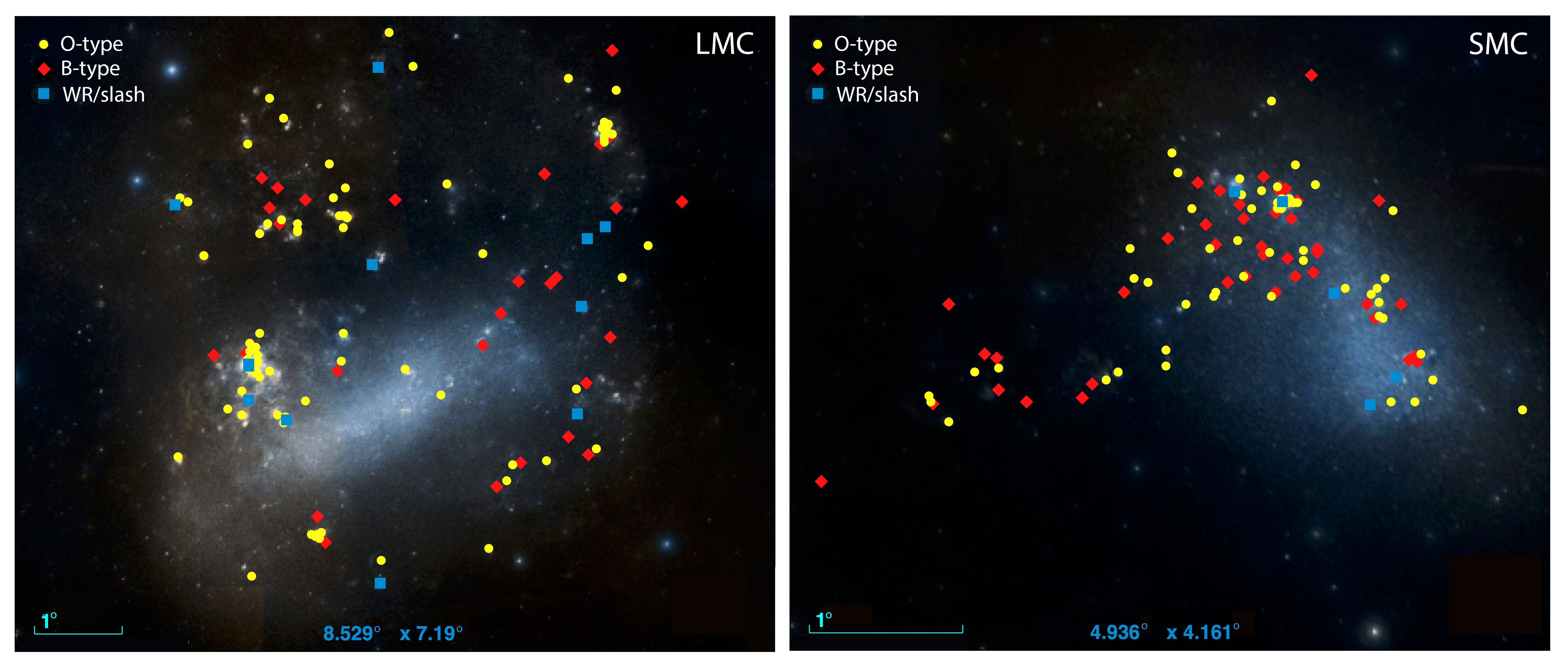
Figure 1: Positions of the ULLYSES/XShootU sources in the LMC (left) and SMC (right). Yellow dots are O-type stars, red diamonds are B-type stars, and blue squares are Wolf-Rayet (WR) and WR-like Of/WR ”slash” stars. We note that the two images have different spatial scales. This figure was made with the Aladin Sky Atlas (Bonnarel et al. 2000); the background consists of DSS2 colour images.

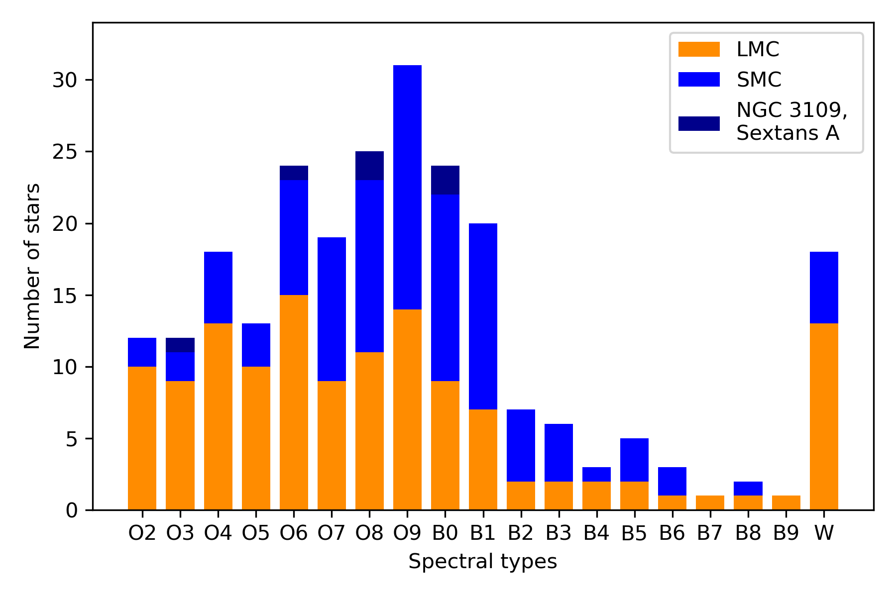
Figure 2: Distribution of the spectral types in ULLYSES. For the 10 known binaries in the sample only the primary component is accounted for. The category labeled ‘W’ includes Wolf-Rayet (WR) and WR-like ”slash” stars.

The Hubble Space Telescope (HST) has dedicated 1000 Orbits to the Director’s Discretionary Time project “Ultraviolet Legacy Library of Young Stars as Essential Standards” (ULLYSES; Roman-Duval et al. 2020),, making this the largest HST program ever conducted. ULLYSES compiles an ultraviolet (UV) spectroscopic Legacy Atlas of about 250 OB stars in low $Z$ regions. Due to their proximity, the Large and Small Magellanic Clouds (LMC, SMC) are the best low-$Z$ laboratories for massive star studies, with respectively 50% and 20% $Z_{\odot}$. They are ideal to study spatially resolved populations of low-$Z$ massive stars to make a leap towards understanding the Early Universe. As a pilot study, several stars at sub-SMC metallicities (in Sextans A and NGC 3109; $\sim$10% $Z_{\odot}$) are also included. The aim is to uniformly cover all spectral sub-types O2$-$B9 and to observe all luminosity classes with spectral types O2$-$B1.5, for both LMC and SMC metallicity, leading to $\sim 250$ stars (Figures  1 and 2).

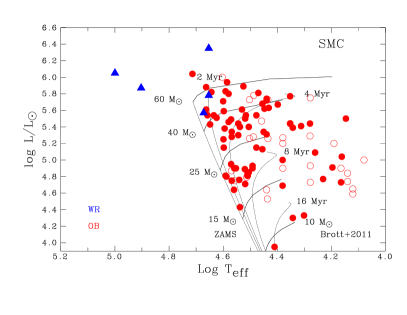
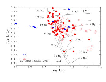
Figure 3: HR diagrams of the ULLYSES SMC and LMC targets. Stellar parameters are based on contemporary literature from Table LABEL:table:params (filled symbols) or spectral type calibrations (open symbols). For known binary/multiple systems, only primaries are indicated. Calibrations used are Doran et al. (2013) for O-type stars in both galaxies, Dufton et al. (2019), Trundle et al. (2004), Trundle & Lennon (2005) for SMC B-type stars and Dufton et al. (2018), Garland et al. (2017), McEvoy et al. (2015a), Urbaneja et al. (2017) for LMC B-type stars. Evolutionary tracks (solid lines) and isochrones (dotted lines) for non-rotating massive stars at 0.5 $Z_{\odot}$ and 0.2 $Z_{\odot}$ are from Brott et al. (2011), supplemented by tracks for very massive stars in the LMC from Köhler et al. (2015).

Although massive stars emit the bulk of their light at UV wavelengths, the optical region remains the cornerstone of spectroscopic analysis studies. The UV regime is powerful to determine the iron (Fe) abundance and to obtain information on wind parameters, such as the terminal velocity ($v_{\infty}$). The optical regime is crucial to determine the basic stellar parameters, such as effective temperature ($T_{\rm eff}$), surface gravity ($\log g$), and abundances (Hillier 2020, Simón-Díaz 2020, Brands et al. 2022) Key information on wind clumping and mass-loss rates ($\dot{M}$) only become reliable when optical and near-infrared (NIR) observations are added. Knowledge of the NIR regime is also critical for observations with instrumentation at the James Webb Space Telescope (JWST) and the Extremely Large Telescopes, which will predominately shift our focus to longer wavelengths. Despite the great potential of ULLYSES to transform our knowledge of massive stars, this Legacy dataset is not complete without observations in the optical and NIR regimes. Thus, the XShootU project was conceived to obtain complementary high quality spectra of the ULYSSES targets with X-shooter at ESO’s Very Large Telescope (Vernet et al. 2011).

The optical Large VLT-Flames Survey of massive stars (PI: S.J. Smartt) and its successor, the VLT-Flames Tarantula survey VFTS (PI: C.J. Evans), tackled many science questions including the $Z$-dependence of stellar wind mass-loss rates (Mokiem et al. 2007b) and the rotation velocities of massive stars (Ramírez-Agudelo et al. 2013). The surface nitrogen (N) abundance of most massive stars in the MCs seemed to be consistent with theoretical predictions, but a significant fraction of stars ($20\%-40$% depending on sample and metallicity) showed chemical enrichment that is either too strong or too weak (e.g., Hunter et al. 2008a, Przybilla et al. 2010, Maeder et al. 2014, Grin et al. 2017).

The absolute mass-loss rates of massive OB and Wolf-Rayet (WR) stars are still uncertain (e.g., Sundqvist et al. 2019, Sander et al. 2020, Ramachandran et al. 2019, Marcolino et al. 2022, Rickard et al. 2022). According to evolutionary models, the bulk of the mass loss could occur during the B-supergiant phase rather than during the preceding O-star phase (Groh et al. 2014). The $Z$ dependence of mass-loss behaviour in this cooler regime is highly complex, involving various mass-loss discontinuities as a function of temperature (bi-stability jumps; Petrov et al. 2016), and is critical in predicting BH masses as a function of $Z$ (Belczynski et al. 2010) as well as GW mergers (Kruckow et al. 2016).

The combined UV and optical XShootU project was motivated to address these science questions as well as a large variety of additional questions concerning massive stars at low $Z$. The project will derive accurate stellar and wind parameters, such as effective temperatures, luminosities, gravities, abundances, and mass-loss rates. This will establish whether mass-loss rates are decreasing with lower $Z$, as predicted (Vink et al. 2001, Kudritzki 2002) and empirically supported for relatively small LMC and SMC VLT-Flames survey samples (Mokiem et al. 2007b, Ramachandran et al. 2019). Moreover, feedback parameters involving wind momenta, wind kinetic energy, and ionising fluxes are key ingredients for building the next generation of spectral population synthesis models that may be applied to extra-galactic surveys, such as CLUES (Sirressi et al. 2022), CLASSY (Berg et al. 2022), the HST spectroscopic survey of star-forming galaxies in the Local Universe, and future projects. Bright early-type stars are also excellent probes of ISM conditions (van Loon et al. 2013). We expect many spin-off projects using XShootU and ULLYSES data, including the derivation of the extinction law for which X-shooter’s wide spectral range is particularly useful.

In this work, we present the XShootU project. The science requirements are described, as well as initial results on data reduction and data analysis processes. We show how the legacy spectroscopic data-set of ULLYSES and XShootU can increase our knowledge of massive stars at low $Z$. The organisation of the XShootU collaboration is described in the Appendix. Already published data (Table LABEL:table:params, plotted in Fig. 3) may naively suggest that properties of LMC and SMC stars are known, but these pre-ULLYSES results have been derived for relatively small and heterogeneous data-sets, and gaps are evident. To make matters worse, spectral analyses to derive the stellar properties have also been heterogeneous, as different authors have not only used different tools, distances, and baseline abundances, but also different wavelength ranges.

To make progress, not only the spectroscopic data sets need to be uniform – as provided by ULLYSES and XShootU – but so does the spectral analysis approach. To give an example, to determine the $\dot{M}-Z$ relationship not only require accurate mass-loss rate determinations, but also reliable stellar parameters, such as luminosities, to compare $\dot{M}$ from one star with one set of stellar properties in one particular galaxy to the mass-loss rate from another star in another galaxy. A uniform data and analysis approach is at the heart of the XShootU project.

2 XShootU science requirements

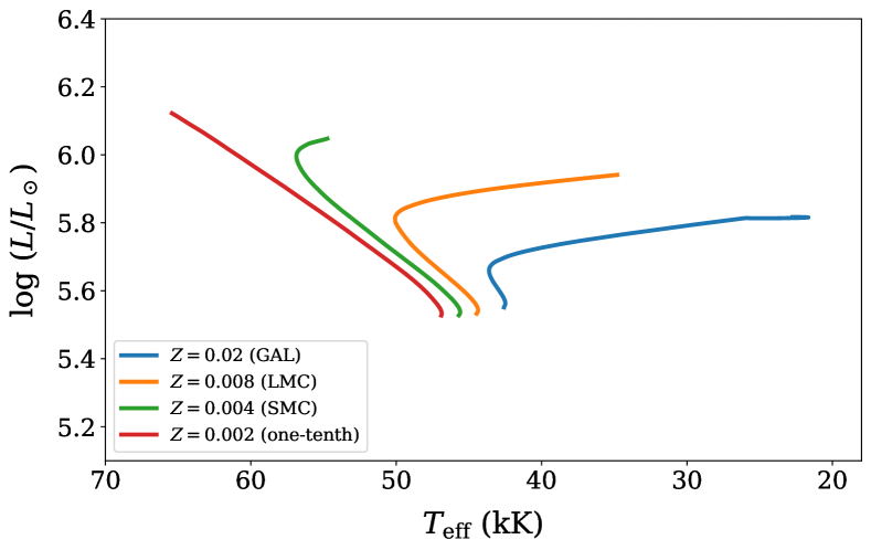
Figure 4: Main-sequence MESA stellar evolution models of a rapidly rotating ($v\sin{i}=550$ km/s) 50 $M_{\odot}$ star for a range of metallicities. The Galactic and LMC model show traditional redwards evolution, while the SMC and even lower $Z$ (1/10th solar) models start to show bluewards chemical homogeneous evolution. The models employ Vink et al. (2000, 2001) mass-loss rates and assume a moderate amount of core overshooting with a value of $\alpha_{\rm ov}$ of $0.335$, similar to Brott et al. (2011) models.

In order to build better population synthesis models of massive stars in low-$Z$ environments, such as those at high redshift studied with JWST, we require (i) more complete spectral libraries, as well as (ii) more reliable stellar evolution models for low-$Z$ stars. The former involves the construction of more accurate model atmospheres, but the latter implies a better handle on the behaviour of wind mass loss over a multi-dimensional parameter space, including $Z$. The key line driver of the inner winds that sets $\dot{M}$ of massive OB stars is iron (Fe), while intermediate mass elements such as CNO dominate the outer winds, setting the terminal velocity (Vink et al. 1999, Puls et al. 2000). While high redshift galaxies may have different [$\alpha$/Fe] ratios compared to local low-$Z$ galaxies, non-solar [$\alpha$/Fe] ratios should have very little impact on the expected mass-loss rate, as long as one correctly interprets low-$Z$ as having low Fe contents (see for instance Table 5 in Vink et al. 2001 for conversions between O and Fe).

One potential concern is whether the local low $Z$ LMC and SMC at 0.5 $Z_{\odot}$ and 0.2 $Z_{\odot}$ are sufficiently metal-poor to gain insight into low-$Z$ stellar evolution in high-redshift galaxies. In order to make the case that the SMC indeed has a sufficiently low Fe-contents to provide key insights into the Early Universe, we showcase a number of MESA stellar evolution models (see WG 5 in Appendix) in Fig. 4. The plot indicates that a rapidly rotating massive star at LMC metallicity still shows classical redwards evolution, just like in the Milky Way, but that already the 1/5th solar SMC metallicity is sufficiently low to undergo bluewards chemically homogeneous evolution (CHE), similar to even lower $Z$ stars at 1/10th solar. The Galactic model loses as much as a third of its initial 50 $M_{\odot}$ mass already on the main-sequence, while the SMC and lower-$Z$ models lose of order 10% or less. Moreover, while the Galactic and LMC models completely spin down during the main sequence (the Galactic model drops below the minimum observable $v\sin{i}$ value of 100 km/s after 3 Myrs, while the LMC star can delay this to 4.5 Myrs), the SMC and lower $Z$ models hardly spin down at all. In fact, the SMC and lower $Z$ model evolve towards critical rotation, rather than away from it. In other words, the SMC is an ideal test-bed for gaining an understanding of the physical difference between the high-$Z$ and the low-$Z$ Universe.

The results displayed in Fig. 4 may naively give the impression that stellar evolution is already well understood, but this is not the case, and the stellar evolution and population synthesis models are only as good as the input physics. In this parameter space those are predominately given by the assumed amounts of interior mixing and wind mass loss. It is commonly assumed that the only parameters setting the mass-loss rate are the stellar luminosity and the metallicity, but in the oft-used mass-loss recipe of Vink et al. (2000; 2001) parameters such as stellar mass, and effective temperature – including the B supergiant regime below the bistability jump – also play a crucial role. Therefore, in order to make progress on the accuracy of stellar evolution models at low $Z$ we firstly require large samples of wind parameters offered by the ULLYSES sample. Secondly, in order to test these in different parts of the HR diagram, the underlying stellar parameters also need to be robust. Thirdly, in order to test the role of rotational mixing for a range of metallicities we require stellar abundances.

Starting with the third requirement, massive stars undergo H-buring via the CNO cycle, and in the first instance the core nitrogen (N) abundance is expected to increase by an order of magnitude at the expense of carbon (C) (Brott et al. 2011, Ekström et al. 2012). Mixing can bring enhanced N to the surface, which is especially relevant for testing the physics of rotational mixing in stellar evolution models. Factors 2-10 in N enhancement and C depletion are realistically measurable from UV and optical spectroscopy as discussed in Sect. 4. For the stellar parameters, effective temperatures need to be accurate to within 5-10%, which is routinely achieved in non-LTE model atmosphere modelling. More cumbersome is the estimated $\log g$ that determines the spectroscopic mass. In Sect. 4 we show that in order to be able to derive accurate $\log g$ the UV alone does not suffice, and optical Balmer lines are mandatory (see below). Arguably the least well-constrained parameter is the wind mass-loss rate. While UV P Cygni lines offer relatively accurate values of the terminal wind velocity, $\sim$10% (Prinja et al. 1990), uncertainties in empirical mass-loss rates are about an order of magnitude due to the roles of respectively micro-clumping and macro-clumping (Fullerton et al. 2006, Oskinova et al. 2007, Sundqvist et al. 2018) Clearly such huge uncertainties are not acceptable when building reliable stellar evolution and populations synthesis models. From our experience in stellar modelling, such as the experiments performed in Fig. 4, we conclude that we need the mass-loss rate to be accurate to 0.3 dex.

As the mass-loss rate is a multi-variate function of stellar parameters, such as $L$, $M$, and $T_{\rm eff}$, the accuracy requirements on the stellar parameters need to be at least as good as those for the mass-loss rate. Accuracies on $T_{\rm eff}$ are easily within 10%, though precisions of 1 kK are sometimes quoted. Similarly, $\log{L}$ precisions of 0.1 dex are feasible. However, the real culprit is the stellar mass $M$ which can be obtained from $\log g$ spectroscopically, but which has a long history of uncertainty, culminating in systematic differences between these spectroscopic masses and evolutionary masses of the order of a factor $\sim$2 (Herrero et al. 1992). In Sect. 4 we show that the optical regime is absolutely critical to measure $\log g$.

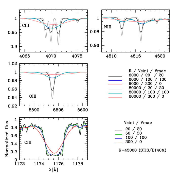
Figure 5: Effect of spectral resolution and rotational velocity on three sets of optical lines classically used to determine C, N, and O abundances. In each panel, the initial cmfgen model has T${}_{\rm eff}=31\,000$ K, $\log g=3.6$ and 0.2 $Z_{\odot}$. The model is degraded to a resolution of either 6000 (typical for our X-shooter UVB spectra) or 80 000 and further convolved with three rotational velocities (20, 100, and 300 km s^-1). No additional macro-turbulent broadening is considered. Also plotted is the UV C iii 1176 line. Here the spectral resolution is that of the STIS E140M grating ($R\sim 45\,000$).

3 XShootU data description

3.1 Target selection

The first objective of the XShootU project is to create a homogeneous legacy atlas of similar quality and scope as that of ULLYSES. The target sample contains 132 LMC stars, 106 SMC targets, and 6 very-low-$Z$ stars in Sextans A and NGC 3109 (Roman-Duval et al. 2020; Table LABEL:table:targets this paper).

Most ULLYSES targets are O-type stars (154), but B-type stars (72) and WR/Slash stars (18) are also included. Figure 1 displays the positions of the targets on the sky and Figure 2 shows the distribution of spectral types. The SMC targets have masses in the range of $10-60\leavevmode\nobreak\ M_{\odot}$, whereas the LMC targets have masses in the range of $15-150\leavevmode\nobreak\ M_{\odot}$. A subset of the ULLYSES targets have previously been spectroscopically analysed (see Table LABEL:table:params). These heterogeneous pre-ULLYSES data are presented in the Hertzsprung-Russell (HR) diagram in Figure 3 (filled symbols). Estimated parameters for targets lacking contemporary analyses are also shown (open symbols).

XShootU obtained a complementary data-set over the optical to NIR wavelength range for all ULLYSES targets that have not previously been observed with X-shooter. This resulted in a sample of 129 LMC stars and 103 SMC stars. In addition, three very low-$Z$ stars were included in the sample.

The ULLYSES and XShootU data-sets are not taken simultaneously in time, although, apart from a few exceptions, the vast majority of ULLYSES sources are not known variables. In reality, most stars are variable to some level, so care still needs to be taken when interpreting the data, but we do not anticipate this to be a massive issue. Existing ESO Science Archive Facility data are part of both spectroscopic and time-dependent aspects of XShootU. Over half of the ULLYSES targets have no previous high-quality optical spectra. Several have been observed with UVES (15%) and/or FLAMES ($\sim$50%), but the wavelength coverage of these FLAMES data is limited. Using (limited) time-sequence data, we will search for binary signatures, and in some cases be capable of disentangling spectra of multi-component systems (Mahy et al. 2020).

3.2 XShootU observing strategy

3.2.1 Wavelength Coverage

ULLYSES obtained moderate resolution spectra of OB stars with selected wavelength settings of the COS G130M, COS G160M, STIS E140M, COS G185M, and STIS E230M gratings in the far- and near-UV during HST cycles $27-29$. In order to complement this UV range, similar quality optical/NIR spectroscopy was carried out with the X-shooter instrument. This slit-fed (11″ slit length) spectrograph provides simultaneous coverage of the wavelength region between $300-2500$ nm, divided into three arms; UVB ($300\lesssim\lambda\lesssim 500$ nm), VIS ($500\lesssim\lambda\lesssim 1000$ nm), and NIR ($1000\lesssim\lambda\lesssim 2500$ nm). X-shooter’s wide wavelength coverage made it the instrument of choice for the purpose of building an optical-NIR legacy data-set.

3.2.2 Spectral Resolution

The X-shooter slit widths were chosen to obtain a spectral resolution of $R=5000-10\,000$, required for estimating the stellar parameters. Each target was observed with a set of $0\hbox to0.0pt{.\hss}^{\prime\prime}8$ (UVB, $R=6700$), $0\hbox to0.0pt{.\hss}^{\prime\prime}7$ (VIS, $R=11\,400$), and $0\hbox to0.0pt{.\hss}^{\prime\prime}6$ (NIR, $R=8100$) slit widths, matching also the average seeing conditions on Paranal. The slit position angle was set by default to parallactic angle, but when necessary a fixed position angle on the sky was used to optimally avoid nearby sources from entering the slits.

Figure 5 illustrates that although the spectral resolution is only medium, the determination of surface abundances, including nitrogen (N), carbon (C), and oxygen (O) should be feasible. It is the projected rotational velocity of some of the stars that will limit such studies. The higher $v\sin i$, the broader the lines, which become challenging to identify at very high $v\sin i$. Even with a S/N around 100 (see justification below) most lines would be undetectable at high $v\sin i$. On the other side of the distribution, lines are only partially resolved at low $v\sin i$. Consequently, the determination of accurate low $v\sin i$ values is not feasible and additional higher spectral resolution data are needed for this subset (see Appendix WG 11) description of auxiliary Magellan/MIKE data), although the combined analysis of optical and UV lines can partially alleviate this limitation. The bottom panel of Figure 5 illustrates the effect of rotational broadening of C iii 1176, a line complex relevant for the determination of $v\sin i$ (e.g., Bouret et al. 2013). Above 100 km s^-1, the components of the multiplet are blended, while at lower rotational velocities they are resolved individually.

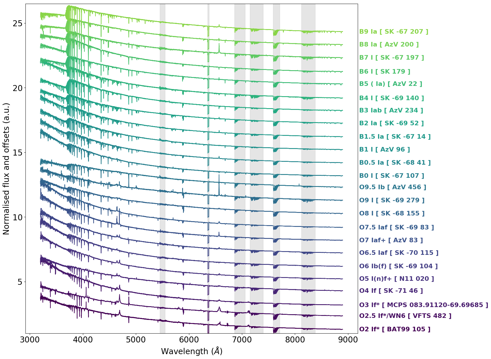
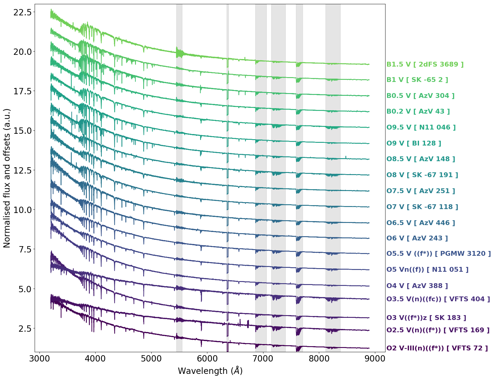
Figure 6: Reduced X-shooter spectra for a range of spectral types of single-star supergiants (top) and dwarfs (bottom). For illustration purposes the flux of each spectrum was divided by its mean value and an arbitrary offset was added. The grey regions correspond to the UVB-VIS common wavelength coverage ($\sim 5500\leavevmode\nobreak\ \AA$), a gap due to bad pixel masking ($\sim 6360\,\AA$), and telluric absorption. Minor manual treatment to remove strong cosmic rays was performed.

Figure 7: Xshooter/UBV spectrum of Sk $--67^{\circ}167$ (O4 Inf$+$) in the LMC, including zoom-in views of key spectroscopic diagnostics.

3.2.3 Signal-to-Noise Ratio

Some VLT instruments provide higher spectral resolution in certain wavelength regimes (e.g., UVES), but to build a homogeneous database with a wide spectral coverage could only be achieved with X-shooter. In addition to the wide wavelength coverage, a high signal-to-noise ratio (S/N) in addition to sufficient spectral resolution are essential to determine the fundamental stellar parameters and the abundances for various temperature regimes populated by OB and WR stars. For the preparation of the X-Shooter proposal, we estimated the required S/N, experimenting on a typical SMC mid-O dwarf/giant with cmfgen model spectra degraded to X-shooter’s spectral resolution. We found that the determination of basic stellar parameters such as $T_{\rm eff}$ and $\log g$ became prohibitive for quantitative interpretation if the S/N drops below $100$ per resolution element. To ensure maximal scientific return of XShootU, we achieved a S/N of $>100$ in the continuum in the UVB and VIS for all MC targets.

3.3 Data Reduction

A detailed description of the data reduction is provided in a paper associated with Data Release 1 (DR1; Sana et al. 2023, XShootU II). Here, we provide a brief summary, focusing on the UVB and VIS spectra. The data reduction of the NIR spectra requires additional efforts and will become part of DR2.

The initial data reduction was performed using the ESO X-shooter pipeline v3.5.0 (Goldoni 2011). The pipeline carried out the standard steps of bias, flat, wavelength calibration, spectral rectification, cosmic ray removal, sky subtraction, flux calibration, and extraction of a 1D spectrum. The wavelength calibration was performed using a physical model, i.e., the transformation from pixel to lambda space was optimized through the analysis of a multi-pinhole ThAr (UVB, VIS) or penray (NIR) lamp frame. The predicted positions of the lines were fitted using a 2D Gaussian to recover the actual positions on the frame.

The pipeline-reduced data were subsequently flux calibrated using a set of 6 standard stars observed during the same or adjacent nights. We found that the stellar models used by the public pipeline (Moehler et al. 2014) resulted in small (on the order of a few percent) changes in the Balmer line profiles depending on the standard star. This potentially impedes accurate $\log g$ measurements. In addition, the spectral energy distribution for some of the standard stars could be optimized. We decided to use new stellar models and new fit points to derive the response, starting with models used by HST for their fundamental flux standards GD 71 and GD 153 (Bohlin et al. 2020). We then reduced observations of the other 5 standard stars taken between October 2020 and April 2021 as if they were science objects, with the response determined by close-in-time observations of GD 71. Those spectra were then co-added to create high S/N spectra that were used to derive improved stellar models. The XShootU spectra were obtained with narrow slits. To obtain absolute flux calibrated spectra, corrections were applied for slit losses due to seeing and image quality across the detector and by re-scaling to existing photometry. The achieved accuracy is typically better than 5%.

Telluric correction was performed using the molecfit tool v3.0.3 (Smette et al. 2015, Kausch et al. 2015) for the VIS arm and generally leads to good results. For the MCs targets, we fitted the atmospheric model directly to the science spectra, as the S/N on the continuum is high enough to ensure a better correction than using a telluric standard star to compute the model. The regions with very deep O₂ telluric absorption lines at $\sim$760 nm and sometimes the one at $\sim$690 nm are poorly corrected and the correction of the H₂O bands at $\sim$950 nm leaves strong residuals. The correction from telluric lines around the [OI] 6300Å line is always good.

Results of the data reduction are shown in Figure 6. Here a sample of reduced X-shooter spectra is presented to highlight a sequence from the earliest to the latest spectral types for supergiant and dwarf targets. The spectra shown are single-epoch in order to avoid confusion in co-added spectra due to potential variability. Telluric correction (grey regions) and proper cosmic-ray removal was not performed for this plot, but will become part of the first data release (Sana et al. 2023, XShootU II). An example of an O4 supergiant spectrum is shown in Fig. 7 on a improved scale, focused on wavelength regions in which telluric corrections are not needed.

4 Multi-wavelength analyses

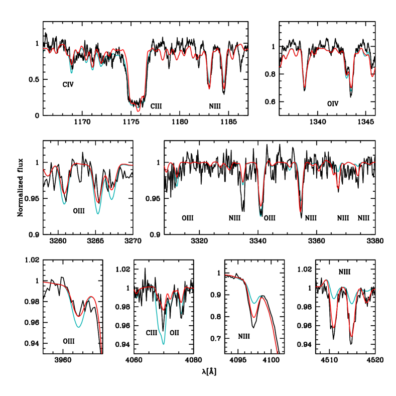
Figure 8: Comparison between the observed HST (top) and X-shooter spectrum (black line) of selected lines of C, N and O lines for AzV 327 (O9.5 II-Ibw) with two models (colored lines). The light blue line is for solar-scaled abundances (factor 1/5) while the red model has the following scaling: C abundance decreased by a factor 3.8, N abundance increased by a factor 4.5, and the O abundance decreased by a factor 1.6. The models were computed with the non-LTE CMFGEN (Hillier & Miller 1998) atmosphere code.

In Sect. 2 we showed that the low-$Z$ environment of the SMC can be considered rather characteristic of the Early Universe, with low mass-loss rates, and the potential for rapid rotation and bluewards evolution, while the LMC sample is more characteristic of today’s Universe, with higher mass-loss rates, slower rotation, and classical redwards stellar evolution. In reality, the situation is more complex, as the mass-loss rates is a function of $\dot{M}=f(Z,L,M,T_{\rm eff},v\sin{i})$, which implies we need to obtain stellar and wind parameters over a large parameter space, including not only the O-star regime, but also the B supergiant regime, where the bi-stability jump may increase mass-loss rates (Vink et al. 1999), or not (Björklund et al. 2021). Moreover, stellar evolution models depend on interior mixing, and stellar abundances can be utilized to test the efficiency of (rotational) mixing.

4.1 Diagnostics in the UV and Optical range

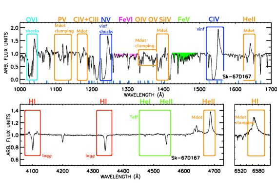
Figure 9: UV (top) and optical (bottom) spectrum of the LMC star Sk-67 167 (O4 Inf+). The UV spectrum consists of STIS E140M observations taken as part of the ULLYSES project and archival FUSE data. The optical spectrum was obtained with X-shooter. A selection of diagnostics for stellar and wind parameters are highlighted. Note that these diagnostics can vary with spectral type. The ticks at the bottom of the UV spectra mark the position of interstellar lines.

To start with the latter, He/H abundances can only be determined from the optical since H/He lines in the UV are dominated by strong interstellar features (e.g. Lyman alpha) so the Pickering-Balmer lines in the optical are critical for the He/H ratio.

Abundances of C, N, and O can in principle be determined from the UV range only (e.g. Bouret et al. 2003, 2013) but most lines are also sensitive to winds, especially as one moves away from the main sequence. Fig. 8 shows an example where winds are sufficiently weak for such a determination. The plot also highlights that the optical range contains more lines from these elements, and these lines depend far less on wind properties than those in the UV. Using more lines reduces the systematic uncertainties in the determinations. Figure 8 highlights that it is still challenging to obtain a perfect fit for all lines of the same element, but the availability of more lines helps identifying potential shortcomings in the atmosphere models. It also allows for a better determination of errors associated with abundance determinations, which is crucial to interpret stellar evolution predictions of interior mixing. A full error determination will follow in a dedicated paper, but we could already say that typical error bars are 15-30%, sometimes up to 50%, with these two data-sets combined (see Bouret et al. 2021), easily satisfying our science requirements.

Another key aspect of combining the ULLYSES and XShootU data-sets is that it allows stellar and wind parameters to be derived self-consistently using both optical and UV diagnostics, which was lacking in surveys such as VFTS. For O-type stars, there are no conclusive diagnostics in the UV to derive effective temperatures and gravities. The wind profiles of O iv, O v, and N iv impose a minimum effective temperature, but they are also sensitive to the mass-loss rate and clumping properties. Figure 9 highlights which parameters can be determined from specific UV as well as optical lines for an LMC O supergiant.

As 30% of the sample involves B stars rather than O-type stars, we also show Fig. 10 highlighting which parameters can be determined from the UV versus optical part for B supergiants (Crowther et al. 2006, Firnstein & Przybilla 2012, McEvoy et al. 2015b). The combination of UV and optical spectra is even more powerful to constrain the physical properties of B-type stars. As in the case of O-stars their UV spectrum alone does not contain diagnostics for gravity. Effective temperature could to first order be constrained by comparing the Cii/Ciii lines and the Feiii/Feiv line forests, although the C lines are also sensitive to mass loss, and Fe transitions depend also on $\log g$. The optical range offers cleaner $T_{\rm eff}$ diagnostics from the ionization balance of Siii/Siiii/Siiv (secondarily, the comparison of Hei and Mgii) and gravity (e.g. H$\gamma$ and the higher Balmer lines). The numerous metallic lines in the optical can be used to determine abundances and in the case of the strongest transitions (e.g. Siiii) micro-turbulence, and projected rotational velocity. The joint UV $+$ optical range offers several mass-loss rate and clumping diagnostics, with the Siiv doublet being the best wind velocity indicator for early B supergiants.

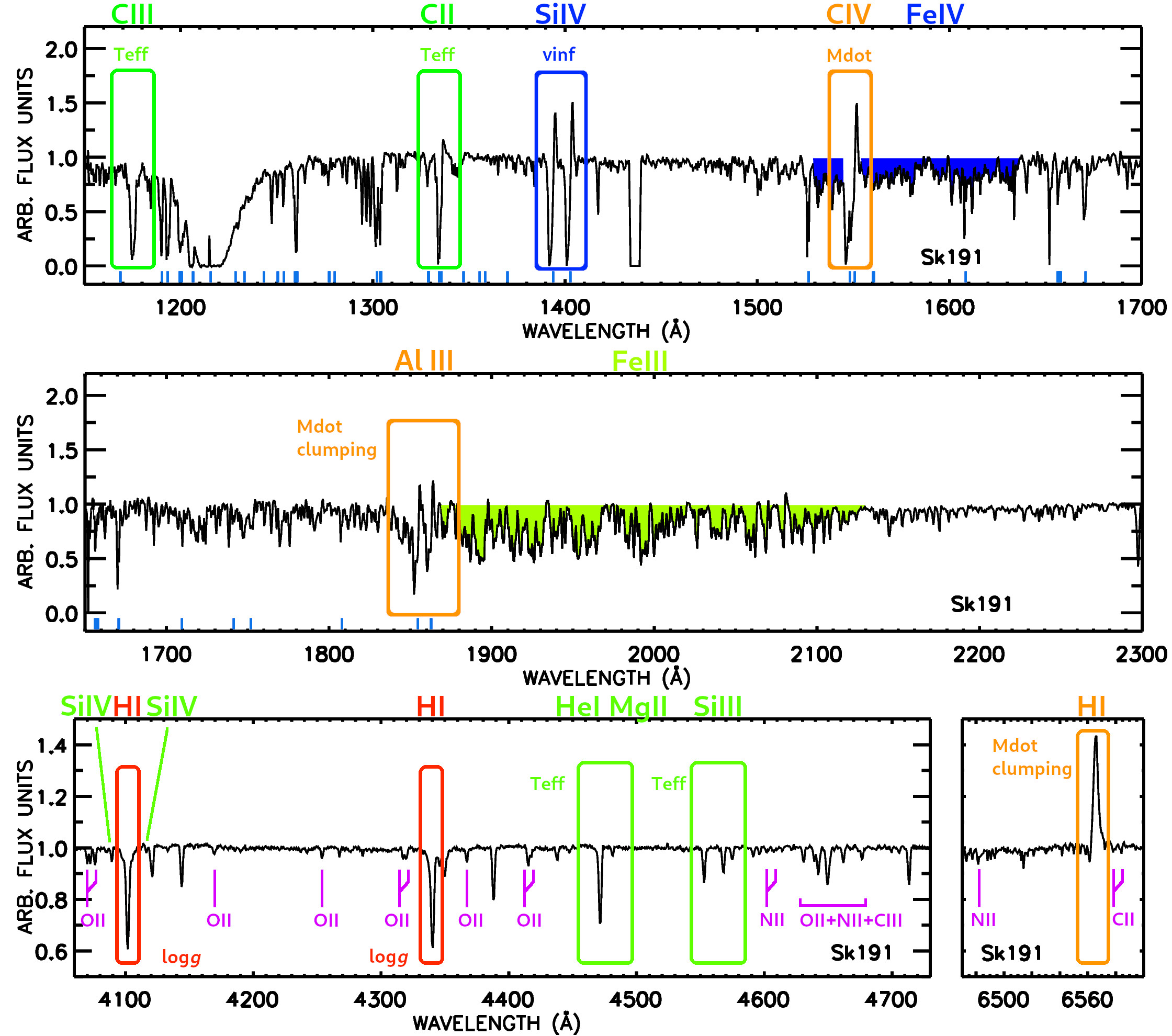
Figure 10: UV (top, middle) and optical (bottom) spectrum of the SMC star Sk191 (B1.5 Ia). The UV spectrum consists of FUSE, STIS E140M and STIS E230M observations compiled as part of the ULLYSES project. The optical spectrum was obtained with X-shooter. Similarly to Fig. 9 interstellar transitions and a selection of stellar and wind diagnostics are highlighted. In addition, metallic lines that can be used to measure abundances are marked in purple.

In order to further quantify the need for optical X-Shooter spectra in spectroscopic analyses, we present an example analysis for an O8 III SMC giant in Figure 11. The figure shows both the UV part of the spectrum and some Hydrogen Balmer lines that are routinely utilized to derive $\log g$ values. It can easily be seen that while high and low $\log g$ model values reproduce the UV spectra equally well, the optical is critical for accurate $\log g$ determination. While the complexity of the spectroscopic analysis is beyond the scope of this paper, the key point is that UV-only fits yield very poorly constrained surface gravities, which result in enormous uncertainties on spectroscopic masses.

In addition to the uncertainty in surface gravity, it is also appropriate to mention that for stars with strong winds, such as supergiants, the H$\alpha$ Balmer line is a key mass-loss and clumping factor diagnostic. When only accounting for micro-clumping and the UV part of the spectrum, Fullerton et al. (2006) showed that clumping factors were uncertain by factors of up to a hundred, and mass-loss rate reductions could easily be an order of magnitude. Only when accounting for the optical H$\alpha$ line and macro-clumping (see Appendix WG 4), Oskinova et al. (2007) showed that mass-loss rate uncertainties were significantly smaller, by a factor of 2 or so, and from the additional optical H$\alpha$ line, clumping factors are usually estimated to be lower of order 6-8 (e.g. Ramirez-Agudelo et al. 2017).

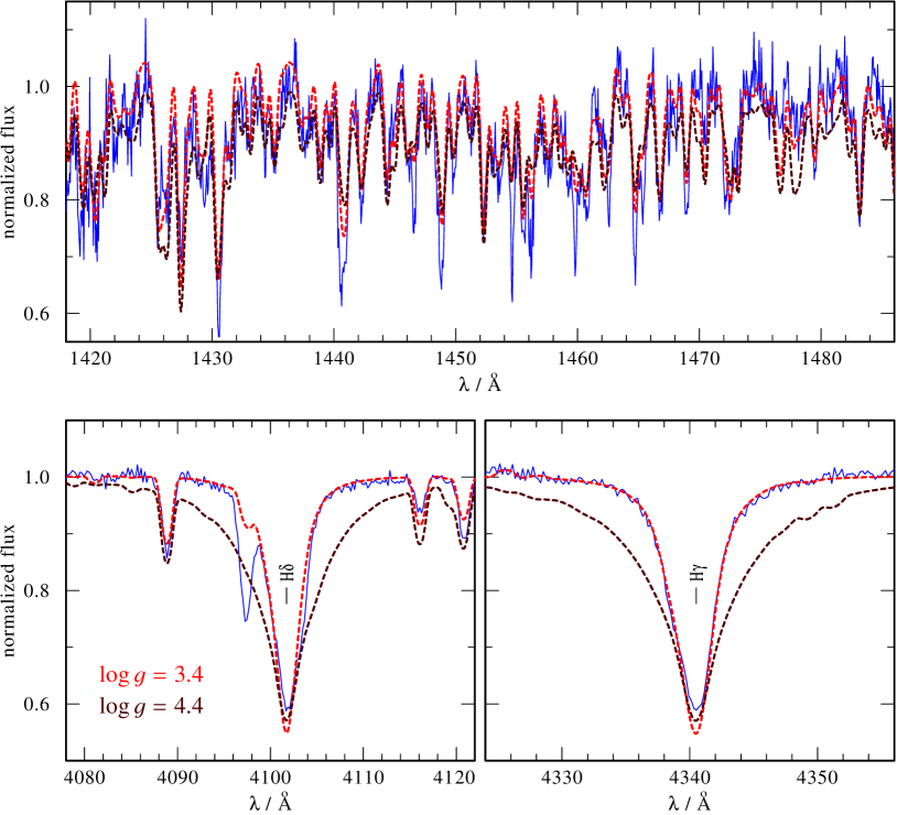
Figure 11: O giant (AV186, O8.5III). The best fitting model is for $T=33$ kK and $\log g=3.4$. Note that while a ten times higher mass star with $\log g=4.4$ would be indistinguishable in the UV, it would completely fail to reproduce the optical Balmer wings. The model was computed with the PoWR (Sander et al. 2017) non-LTE code.

4.2 Spectroscopic analyses tools and procedures

XShootU is coordinating spectral modelling efforts for massive stars on a world-wide scale never witnessed before in the massive-star community. Before we can scale-up the analysis to hundreds of massive stars with hugely varying spectral and wind properties over the entire hot part of the HR diagram, it is paramount that codes and analysis techniques are tested and compared as a function of stellar parameters and metallicity.

The spectral analysis of massive stars is rather intricate due to the highly non-local thermodynamic equilibrium (NLTE) conditions in their turbulent, supersonic atmospheres. Over the past decades, a number of highly complex, yet successful, model atmosphere codes have been developed, e.g., CMFGEN (Hillier & Miller 1998), PoWR (Hamann & Gräfener 2003, Sander et al. 2015) and FASTWIND (Santolaya-Rey et al. 1997, Puls et al. 2005). Although these codes have previously been applied to various sets of observations, only more recently have they been used for larger samples (e.g., Ramírez-Agudelo et al. 2017, Sabín-Sanjulián et al. 2017) due to the efficiency of numerical methods (applying certain physical approximations), and efficient spectral automated analysis tools including genetic algorithms and grid-based $\chi^{2}$ approaches.

At virtual and on-site Lorentz workshops in 2021 and 2022 (and various additional virtual XShootU meetings) preliminary comparisons of analyses with the various non-LTE codes were performed by modelling subsets of O-stars. Agreement was reached on a common methodology to perform the spectroscopic analyses within the XShootU Project.

This recommended procedure may be summarised as follows:

1. Use the same reference value for the distance moduli (DM) of the LMC and the SMC. We adopted DM(SMC) = 18.98 mag (Graczyk et al. 2020) and DM(LMC) = 18.48 mag (Pietrzyński et al. 2019).

2. Adopt the same photometry ($U,B,V,J,H,K_{\rm S}$, as minimum) for each star (Table LABEL:table:targets). Optical photometry is from a variety of sources, whereas near-IR photometry is from VISTA VMC (JKs) (Cioni et al. 2011a), 2MASS (JHKs) (Cutri et al. 2003a), or 2MASS 6X (JHKs) (Cutri et al. 2012a). H-band photometry is omitted if JKs values are discrepant between 2MASS and VMC owint to photometric variability or crowding.

3. Adopt the same literature source for the bolometric correction. The relation for bolometric correction as a function of $T_{\rm eff}$ and metallicity from Lanz & Hubeny (2003) is adopted for now. This relation may be updated in the course of this project.

4. Adopt the same reddening approach. Key references for the Milky Way foreground are Fitzpatrick et al. (2019), over earlier works by Seaton (1979), Cardelli et al. (1989), though Galactic foreground extinction is modest towards the MCs.

   For the MC contributions, Gordon et al. (2003) is preferred, recognising earlier contributions from e.g. Howarth (1983), Fitzpatrick (1986) to UV laws in the LMC, and for the SMC e.g. Prevot et al. (1984), Bouchet et al. (1985) to the UV and optical/IR respectively. For the FUSE range, Gordon et al. (2009) and Cartledge et al. (2005) are recommended for the Milky Way, and MCs, respectively.

5. Adopt the same baseline LMC and SMC abundances. Several abundance ratios in the MCs are notoriously non-solar, which is especially true for CNO in the SMC, and the use of scaled-solar values should be avoided when possible. Thus, the adopted abundance values were derived from an average of different determinations, e.g., from stars, H ii regions, and SN remnants. The recommended values are listed in Tables 2 and 3. For several species, however, we need to agree on default abundances, given the absence of lines in spectral ranges covered by ULLYSES $+$ XShootU. In such cases, scaled-solar values need to be adopted, using 0.5 $Z_{\odot}$ and 0.2 $Z_{\odot}$ scaling factors for the LMC and SMC, respectively (Asplund et al. 2009).

6. Whenever possible, adopt the same description of macro-turbulence for line broadening. The recommendation is to adopt a radial-tangential description of macro-turbulence (e.g., Simón-Díaz & Herrero 2014).

7. Adopt similar wind clumping implementation. We agreed to use the same parametric description as implemented in CMFGEN (Hillier & Miller 1998) for the standard derivation of the mass-loss rate. Clumping is predominately treated in the “microclumping” approximation, assuming a void interclump medium. The volume filling factor $f_{\text{V}}$ has a velocity-dependent behavior that goes as:

   $$f_{\text{V}}(r)=f_{\text{V},\infty}+(1-f_{\infty})\,e^{-\varv(r)/\varv_{\text{cl}}}$$ (1)

   where $f_{\text{V},\infty}$ denotes the value at $r\rightarrow\infty$. For a void inter-clump medium, the corresponding clumping factor $D\equiv f_{\text{cl}}$ is simply the inverse value, implying that $D_{\infty}=f_{\text{V},\infty}^{-1}$. The free parameter $\varv_{cl}$ is a characteristic velocity varied to describe the clumping onset. More sophisticated descriptions of the properties and nature of clumping can be implemented in the codes (e.g., Oskinova et al. 2007, Hawcroft et al. 2021, Flores & Hillier 2021). These predominately fall under the framework of WG 4 that focuses on wind structure (see below).

The next step is to benchmark the accuracy of stellar parameters derived with the different approaches. For this, a small set of stars was modelled with various non-LTE codes. The obtained stellar parameters were compared, allowing us to assess to what extent the physical interpretation depends on the modelling tools applied. In parallel, we also considered bench-marking of the non-LTE wind codes, i.e. against one another or against mock data, to perform a direct comparison of synthetic spectra computed for the same input model parameters. Alternatively, we could use a model obtained with one code and fit this model with the other codes. These various ”bench-marking” approaches will provide relevant information of systematic differences between codes, analyses tools, and other differences in approach, which will be detailed in a future (benchmarking) paper (Sander et al. 2023; XShootU IV).

Determination of the wind terminal velocities ($v_{\infty}$) is also taken on. As a global wind parameter, this is indeed an essential input for the models of stellar atmospheres used. The ULLYSES (UV) data are of particular importance for this task as they are rich in resonance transitions of ionised species which are prime $v_{\infty}$ diagnostics. For stars presenting saturated resonance-line UV profiles, considering that the spectral lines remain optically thick at the distances where the wind reaches its maximum speed, $v_{\infty}$ can be measured directly by measuring the maximum velocity shift of the absorption component of the UV C iv resonance doublet (see, e.g., Prinja et al. 1990, Prinja & Crowther 1998). Alternatively, the wind speeds can also be measured by fitting synthetic spectra produced using the Sobolev with Exact Integration (SEI) method (Lamers et al. 1987). This latest approach is particularly relevant for stars without saturation in their UV resonance-line profile (although it can also be used in the first case mentioned above). As this paper is being written, a significant fraction of the LMC and SMC star sample has been studied with either method. Results concerning the dependence of $v_{\infty}$ with the ambient metallicity or stellar parameters will be presented in dedicated papers (e.g. Hawcroft et al., XShootU III).

5 Final Perspectives

The XShootU project is expected to provide many pieces of data, models, as well as new physics of massive stars in low $Z$ environments. It is important to stress that the overarching aim is to provide a high-quality homogeneous optical database that is complementary to ULLYSES. These legacy data-sets are critical for a correct interpretation of unresolved high $Z$ observations with JWST/NIRSPEC (Curti et al. 2023, Carnall et al. 2023, De Barros et al. 2019). The next goal is to provide uniformly determined stellar and wind parameters from the combined UV and optical data-sets. For this part of the project, it is not only critical to include the correct non-LTE physics, but also to test the various spectral synthesis codes and analyses.

A key science aim is to quantify how the mass-loss rate declines with decreasing metallicity. This does not necessarily simply imply a determination of a power-law exponent, as the slope may easily vary with stellar parameters or $Z$ itself (Vink et al. 2001, Kudritzki 2002, Sander & Vink 2020, Marcolino et al. 2022, Rickard et al. 2022). In order to obtain an empirical $\dot{M}=f(Z)$ relationship, we not only require mass-loss rates and clumping properties, but simultaneously also need to obtain the underlying stellar parameters ($T_{\rm eff}$, $\log g$, $L$, $M$) as these parameters enable mass-loss properties from a given object in one galaxy to be compared to those from an entirely different object located elsewhere.

The XShootU data-set, coupled with surveys of H ii regions in the LMC and SMC such as SDSS LVM, represents a significant opportunity to advance the state-of-the-art in our understanding of how stars shape their environment. LVM is an optical ($3600-10000$ Å) integral-field spectroscopic survey ($R\sim 4000$) of the Milky Way and the Local Group (LMC/SMC/M31/M33). It will be the first IFU survey to isolate and resolve distinct environments within galaxies, and to cover significant portions of the night sky. New populations synthesis models – informed by the new physics obtained in the XShootU collaboration – can be used to remove the stellar contribution from LVM observations of star-forming regions, which will enable studies of the ionized-gas alone (H ii regions, diffuse ionized gas), over the large dynamic range in size of LVM, i.e., from clusters and clouds (10-50 pc) to the kpc scales of spiral arms, galactic in/outflows, and disk dynamics.

One should be aware that different communities refer to $Z$ in different ways. Extra-galactic communities usually work on the basis of nebular oxygen (O) lines, while stellar astronomers are sometimes able to derive Fe abundances of individual stars. It is predominately the Fe abundance that sets the mass-loss rate, while intermediate mass elements such as O set the wind terminal velocity (Vink et al. 1999, Puls et al. 2000). While the [$\alpha$/Fe] ratio in Local dwarf galaxies such as IC 1613 is generally found to be sub-solar (Tautvaišienė et al. 2007, Garcia et al. 2014), Steidel et al. (2016) and Strom et al. (2022) showed O to be enhanced in comparison to Fe for galaxies at intermediate redshift (”Cosmic Noon”). This is thought to be due to the time delay in the production of Fe from Type Ia supernovae with respect to $\alpha$ elements released by massive stars. It may therefore become relevant to consider more detailed abundance patterns than simply scaling all metals with the solar-abundance pattern, i.e. to make a clearer distinction between [Fe/H] and $\alpha$ elements for $\dot{M}$ calibrations of massive stars, as indicated in Table 5 in Vink et al. (2001). The ULLYSES and XSHootU sample will uniquely provide the opportunity to investigate potential differences between [Fe/H] and $\alpha$ elements with non-solar patterns.

When we are eventually able to provide a reliable empirical $\dot{M}=f(Z)$ relation we can compare these findings to theoretical predictions, and this will inform us on how to treat mass loss more reliably in models of stellar evolution – and thereby also in feedback and population synthesis studies – at low $Z$. It is currently unclear if most of the mass loss takes place in $Z$-dependent winds, or in $Z$-independent eruptions or binary interactions. Despite the possibility of significant $Z$-independent mass loss, there is ample evidence that massive-star evolution in metal-poor environments proceeds very differently from our Milky Way. Shirazi & Brinchmann (2012) and Kehrig et al. (2015) found strong nebular He ii emission lines in low-$Z$ galaxies, but not in metal-rich ones. Long-duration gamma-ray bursts (GRBs; e.g., Vreeswijk et al. 2004), superluminous SNe (e.g., Quimby et al. 2011, Gal-Yam 2012, Chen et al. 2015), and broad-line Type Ic SNe occur preferentially in low-$Z$ dwarf galaxies (e.g., Palmerio et al. 2019),whereas ordinary Type Ic SNe avoid dwarf galaxies.

The spectacular merger of two $\sim 30\leavevmode\nobreak\ M_{\odot}$ black holes observed through the detection of GWs by the LIGO observatory (Abbott et al. 2016a) most likely originated from a system that had an initial $Z$ similar to that of the SMC (Abbott et al. 2016b). This conclusion is inextricably linked to the predicted reduced stellar wind mass loss at low $Z$ (e.g., Vink et al. 2001). Proposed channels that may have lead to GW 150914 (and other more recent events) involve mass transfer and common envelope evolution (e.g., Belczynski et al. 2016) and “chemically homogeneous evolving” (CHE) systems (Mandel & de Mink 2016). The latter model is linked to rapid spin rates, leading to rotationally-induced mixing of the stellar interior (Maeder 1987, Yoon & Langer 2005). Predictions of single star evolution have shown this process to be increasingly important at lower $Z$ (Brott et al. 2011) due to lower mass-loss rates, and correspondingly less angular momentum loss. Support for the existence of CHE can be found in the properties of a small fraction of WR stars (Martins et al. 2009, Hainich et al. 2015), but CHE still lacks unambiguous observational confirmation in the O-star regime (see for example Walborn et al. 2004, Abdul-Masih et al. 2019; 2021 and Bouret et al. 2013 for candidates).

The properties of GW events and exotic SNe illustrate the key physics involved: spin rates and rotationally-induced mixing, CHE, and wind mass-loss rates. The XShootU sample consists of uniformly estimated spectral parameters, of objects previously classified in the literature to varying extents. Further analysis will include, for instance a determination of an upper limit to the number of chemically-homogeneous evolving (CHE) stars for which three basic observables need to be fulfilled: (i) a peculiar HR diagram location, as chemically homogeneous stars evolve bluewards instead of redwards (ii) higher average $v\sin i$, as they are thought to be caused by rapid rotation, and (iii) special chemical-abundance patterns showcasing chemical mixing.

These are just some of the studies that are being prepared and their results will be published in research articles of the XShootU series. It should be emphasised that some of the analysis is already ongoing, but there is ample space for new parties to join the project.

Moreover, the XShooter data is open to the public and we also plan to make the higher level data products open to the community at large, as these high-quality data have long-term utility for research projects that may not as yet have been foreseen.

Table 1: Photometric, spectroscopic and multiplicity of ULLYSES/XShootU targets, ordered by RA (Magellan/MIKE targets are indicated in the final column). The infrared photometry is drawn from 2MASS ($JHK_{s}$) or VISTA VMC ($JK_{s}$). $H$-band photometry is missing if 2MASS and VISTA are discrepant (presumably due to photometric variability or sensitivity/crowding issues).

Target, Alias	Sp Type	Ref	$U$	$B$	$V$	Ref	$J$	$H$	$K_{s}$	Ref	$(B-V)_{0}$	$E(B-V)$	Ref	$M_{V}$	Binary?	Ref	MIKE?
			(mag)	(mag)	(mag)		(mag)	(mag)	(mag)		(mag)	(mag)		(mag)
SMC targets
2dFS 163	O8 Ib(f)	1	13.84	14.95	15.11	2	15.28	15.31	15.14	3,4	–0.27	0.11	5	–4.21	$\cdots$	$\cdots$	$\cdots$
AzV 6, 2dFS 5002	O9 III	6	12.45	13.36	13.31	7	12.56	11.78	11.73	3,8	–0.26	0.31	5	–6.63	EB	9	$\cdots$
AzV 14, Sk 9	O5 V	10	12.38	13.38	13.55	7	14.25	14.30	14.31	3,8	–0.28	0.11	5	–5.77	$\cdots$	$\cdots$	$\cdots$
AzV 15, Sk 10	O6.5 II(f)	11	11.90	12.93	13.12	7	13.53	13.57	13.60	3,8	$\cdots$	0.10	12	–6.17	$\cdots$	$\cdots$	$\cdots$
AzV 16, Sk 11, R 4	sgB0$[\,$e$]\,$	13	12.29	13.10	12.97	7	12.35	11.73	11.35	3,8	$\cdots$	0.07	14	–6.23	SB2	14	$\cdots$
AzV 18, Sk 13	B2 Ia	6	11.70	12.49	12.46	15	12.47	12.36	12.32	3,8	–0.17	0.20	16	–7.16	$\cdots$	$\cdots$	$\checkmark$
AzV 22, 2dFS 5015	B5 Ia	6	11.53	12.19	12.20	17	12.27	12.20	12.15	3,8	–0.09	0.08	16	–7.03	$\cdots$	$\cdots$	$\checkmark$
AzV 39a, AB 2	WN5ha	18	13.08	14.08	14.26	7	14.67	14.64	14.64	3,4	$\cdots$	0.10	19	–5.03	$\cdots$	$\cdots$	$\cdots$
AzV 43, 2dFS 700	B0.5 III	20	12.80	13.76	13.88	7	14.37	14.33	14.48	3,8	$\cdots$	0.08	12	–5.35	$\cdots$	$\cdots$	$\cdots$
AzV 47	O8 III((f))	11	12.26	13.26	13.44	7	14.13	14.20	14.26	3,8	$\cdots$	0.05	12	–5.70	$\cdots$	$\cdots$	$\cdots$
AzV 61, Sk 32, 2dFS 748	O6 III((f))e	21	12.31	13.36	13.54	7	14.10	13.99	14.07	3,8	–0.27	0.09	5	–5.72	$\cdots$	$\cdots$	$\cdots$
AzV 69, Sk 34	OC7.5 III((f))	11	12.09	13.09	13.27	7	13.76	13.77	13.86	3,8	$\cdots$	0.11	12	–6.05	$\cdots$	$\cdots$	$\cdots$
AzV 70, Sk 35, 2dFS 756	O9.5 Ibw	22	11.27	12.21	12.38	23	12.77	12.79	12.86	3,8	$\cdots$	0.10	24	–6.91	$\cdots$	$\cdots$	$\cdots$
AzV 75, Sk 38	O5 III(f+)	11	11.55	12.55	12.70	7	13.15	13.22	13.22	3,8	$\cdots$	0.14	12	–6.71	$\cdots$	$\cdots$	$\cdots$
AzV 81, Sk 41, AB 4	WN6h	18	12.36	13.25	13.37	7	13.65	13.52	13.44	3,8	$\cdots$	0.09	19	–5.89	$\cdots$	$\cdots$	$\cdots$
AzV 80	O4-6n(f)p	11	12.22	13.19	13.32	7	13.80	13.74	13.87	3,8	–0.28	0.15	5	–6.13	$\cdots$	$\cdots$	$\cdots$
AzV 83	O7 Iaf+	11	$\cdots$	13.45	13.58	11	13.87	13.96	13.90	3,8	–0.27	0.14	5	–5.83	$\cdots$	$\cdots$	$\checkmark$
AzV 85	B1 II-IIIe	25	12.69	13.68	13.75	26	14.50	$\cdots$	14.60	3	–0.24	0.17	16	–5.76	$\cdots$	$\cdots$	$\cdots$
AzV 95	O7 III((f))	11	12.57	13.60	13.78	7	14.17	14.21	14.17	3,8	–0.27	0.09	5	–5.48	$\cdots$	$\cdots$	$\cdots$
AzV 96, Sk 46, 2dFS 801	B1.5 Ia	6	11.54	12.49	12.59	7	12.93	12.98	12.95	3,8	–0.18	0.08	16	–6.64	$\cdots$	$\cdots$	$\checkmark$
AzV 104	B0.5 Ia	6	12.05	13.01	13.17	7	13.65	13.71	13.73	3,8	–0.22	0.06	16	–6.00	$\cdots$	$\cdots$	$\checkmark$
AzV 148	O8.5 V	27	12.92	13.92	14.12	7	14.67	14.78	14.80	3,4	$\cdots$	0.09	28	–5.13	$\cdots$	$\cdots$	$\cdots$
2dFS 999, AB 9	WN3 ha	18	14.13	15.12	15.24	7	15.84	15.92	15.78	3,4	$\cdots$	0.09	19	–4.02	$\cdots$	$\cdots$	$\cdots$
NGC330 ELS 4 = Rob B37	B2.5 Ib	29	$\cdots$	13.26	13.33	29	13.44	13.45	13.46	3,8	–0.15	0.08	16	–5.90	$\cdots$	$\cdots$	$\checkmark$
NGC330 ELS 2 = Rob A2	B3 Ib	29	12.07	12.80	12.87	7	13.07	13.09	13.08	3,8	–0.13	0.06	16	–6.30	$\cdots$	$\cdots$	$\checkmark$
AzV 175, Sk 64	B1 IIw	30	12.61	13.45	13.53	7	13.83	13.87	13.89	3,8	–0.24	0.16	16	–5.95	$\cdots$	$\cdots$	$\checkmark$
AzV 177	O4 V((f))	31	13.27	14.32	14.53	7	15.15	15.23	15.29	3,4	$\cdots$	0.08	28	–4.70	$\cdots$	$\cdots$	$\cdots$
AzV 186, NGC330 ELS 13	O8.5 III((f))	21	12.75	13.77	13.98	7	14.45	14.47	14.51	3,8	–0.27	0.06	5	–5.19	$\cdots$	$\cdots$	$\cdots$
AzV 187, Sk 68	B3 Ia	6	11.21	11.96	12.06	15	12.29	12.23	12.29	3,8	–0.13	0.03	16	–6.13	$\cdots$	$\cdots$	$\checkmark$
AzV 189, 2dFS 5096	O9 V	27	13.32	14.26	14.37	7	14.92	15.09	15.06	3,8	$\cdots$	0.14	28	–5.03	$\cdots$	$\cdots$	$\cdots$
AzV 200, Sk 69	B8 Ia	6	11.72	12.24	12.17	15	12.10	11.88	11.89	3,8	–0.01	0.08	16	–7.06	$\cdots$	$\cdots$	$\checkmark$
NGC346 ELS 43 = MPG 11	B0 V	29	14.06	15.05	15.18	7	15.77	15.84	15.89	3,4	–0.30	0.17	16	–4.33	$\cdots$	$\cdots$	$\cdots$
NGC346 ELS 26 = MPG 12	O9.5–B0 V (N str)	11	13.77	14.68	14.76	7	15.26	14.98	15.36	3,4	$\cdots$	0.13	28	–4.64	$\cdots$	$\cdots$	$\cdots$
NGC346 ELS 28 = MPG 113	OC6 Vz	11	13.56	14.62	14.78	7	15.46	15.52	15.62	3,4	$\cdots$	0.09	28	–4.47	$\cdots$	$\cdots$	$\cdots$
AzV 207	O7 III((f))	21	12.99	14.05	14.25	7	14.79	14.84	14.94	3,4	–0.27	0.07	5	–4.95	$\cdots$	$\cdots$	$\cdots$
AzV 210, Sk 73	B1.5 Ia	6	11.73	12.58	12.6	7	12.80	12.77	12.79	3,8	–0.18	0.16	16	–6.88	$\cdots$	$\cdots$	$\checkmark$
NGC346 ELS 50 = MPG 299	O8 Vn	29	13.93	15.09	15.25	7	16.05	16.37	16.22	3,4	$\cdots$	0.05	28	–3.88	$\cdots$	$\cdots$	$\cdots$
AzV 215, Sk 76, 2dFS 1352	BN0 Ia	6	11.64	12.60	12.69	7	13.01	12.99	13.04	3,8	–0.24	0.15	16	–6.76	$\cdots$	$\cdots$	$\cdots$
NGC346 ELS 7 = MPG 324 = W6	O4 V((f))	32	12.73	13.78	14.02	33	14.53	14.66	14.68	3,4	$\cdots$	0.07	28	–5.08	$\cdots$	$\cdots$	$\cdots$
NGC346 MPG 355 = W3	ON2 III(f*)	34	12.15	13.27	13.50	33	13.98	14.11	14.14	3,4	$\cdots$	0.07	28	–5.70	$\cdots$	$\cdots$	$\cdots$
NGC346 MPG 368	O6 V	35	12.87	13.95	14.18	33	14.63	14.59	14.78	3,4	$\cdots$	0.07	28	–5.01	$\cdots$	$\cdots$	$\cdots$
NGC346 MPG 435 = W1	O4 If+O5-6	36	11.20	12.21	12.43	37	13.01	13.02	13.11	3,8	–0.28	0.06	5	–6.74	SB2	36,38	$\cdots$
NGC346 ELS 51 = MPG 523	O7 Vz	29	14.20	15.25	15.51	29,33	16.01	16.07	16.16	3,8	$\cdots$	0.05	28	–3.62	$\cdots$	$\cdots$	$\cdots$
AzV 224, NGC346 ELS 8	B1 III	28	13.02	13.97	14.12	7	14.55	14.62	14.56	3,8	–0.26	0.11	16	–5.20	$\cdots$	$\cdots$	$\cdots$
HD 5980, AzV 229, R 14, Sk 78, AB 5	WN6h+WNE+O	18	10.63	11.63	11.83	15	11.11	11.01	10.77	8	$\cdots$	0.08	39	–7.30	SB2	40	$\cdots$
NGC346 ELS 13 = MPG 782	O9 V+B1	41	13.36	14.28	14.46	33	14.95	$\cdots$	15.05	3	–0.27	0.09	5	–4.80	SB2,EB	41,44	$\cdots$
NGC346 ELS 46	O7 Vn	29	$\cdots$	15.16	15.44	29	15.91	15.81	16.08	3,4	$\cdots$	0.04	28	–3.66	$\cdots$	$\cdots$	$\cdots$
AzV 232, Sk 80, NGC 346 ELS 1 = MPG 789	O7 Iaf+	42	11.15	12.15	12.35	15	12.64	12.67	12.67	3,8	$\cdots$	0.05	12	–6.79	$\cdots$	$\cdots$	$\cdots$
AzV 234, Sk 81	B3 Iab	36	12.02	12.84	12.94	7	13.19	13.15	13.22	3,8	–0.13	0.03	16	–6.13	$\cdots$	$\cdots$	$\checkmark$
AzV 235, R 17, Sk 82	B0 Iaw	43	11.07	12.02	12.20	23	12.41	12.32	12.28	3,8	$\cdots$	0.07	24	–7.00	$\cdots$	$\cdots$	$\cdots$
NGC346 ELS 35, 2dFS 1418	B1 V	29	13.83	14.70	14.89	7	15.48	15.73	15.63	3,4	–0.26	0.07	16	–4.31	EB	44	$\cdots$
NGC346 ELS 25 = MPG 848	O9 V	29	13.67	14.67	14.91	33	15.47	15.59	15.63	3,4	–0.27	0.03	5	–4.16	$\cdots$	$\cdots$	$\cdots$
NGC346 ELS 31	O8 Vz	29	13.65	14.74	14.96	7	15.59	15.67	15.75	3,4	$\cdots$	0.09	28	–4.30	$\cdots$	$\cdots$	$\cdots$
AzV 238	O9.5 III	11	12.49	13.47	13.64	7	14.25	14.26	14.35	3,8	–0.26	0.09	5	–5.62	$\cdots$	$\cdots$	$\cdots$
AzV 243, Sk 84	O6 V	32	12.63	13.67	13.84	7	14.43	14.43	14.55	3,8	$\cdots$	0.10	28	–5.44	$\cdots$	$\cdots$	$\cdots$
AzV 242, R 18, Sk 85	B0.7 Iaw	43	11.03	11.95	12.06	15	12.42	12.33	12.38	3,8	–0.19	0.08	16	–7.17	$\cdots$	$\cdots$	$\cdots$
AzV 251	O7.5 V	21	13.32	14.34	14.52	7	15.20	15.18	15.33	3,4	–0.27	0.09	5	–4.74	$\cdots$	$\cdots$	$\cdots$
AzV 255, Sk 90	O8 V	27	11.58	12.59	12.78	15	13.47	13.41	13.13	3,8	–0.27	0.08	5	–6.45	$\cdots$	$\cdots$	$\cdots$
AzV 261, 2dFS 1527	B2 Ibe	1	12.90	13.81	13.88	7	13.81	13.95	13.43	3,8	–0.16	0.09	16	–5.38	$\cdots$	$\cdots$	$\cdots$
AzV 264, Sk 94	B1 Ia	6	11.33	12.24	12.37	15	12.75	12.76	12.75	3,8	–0.19	0.06	16	–6.80	$\cdots$	$\cdots$	$\checkmark$
AzV 266, Sk 95, 2dFS 1545	B1 I	21	11.47	12.43	12.55	7	12.88	12.91	12.91	3,8	–0.19	0.07	16	–6.65	$\cdots$	$\cdots$	$\checkmark$
AzV 267	O8 V	21	13.53	14.58	14.84	7	15.51	15.77	15.64	3,4	$\cdots$	0.05	28	–4.29	$\cdots$	$\cdots$	$\cdots$
AzV 296	O7.5 V((f))	10	13.05	14.07	14.26	7	14.90	14.91	15.00	3,4	–0.28	0.09	5	–5.00	$\cdots$	$\cdots$	$\cdots$
AzV 304	B0.5 V	45	13.74	14.66	14.77	7	15.44	15.50	15.56	3,4	–0.28	0.17	16	–4.74	$\cdots$	$\cdots$	$\checkmark$
AzV 307	O9 III	30	12.82	13.8	13.96	7	14.53	14.69	14.63	3,8	$\cdots$	0.10	12	–5.33	$\cdots$	$\cdots$	$\cdots$
AzV 314	B5 Iab	6	11.98	12.77	12.87	7	13.19	13.19	13.23	3,8	–0.10	0.00	16	–6.11	$\cdots$	$\cdots$	$\checkmark$
AzV 321, 2dFS 1720	O9 IInp	46	12.54	13.57	13.76	7	14.32	14.38	14.41	3,8	–0.26	0.07	5	–5.44	$\cdots$	$\cdots$	$\cdots$
AzV 324	B4 Iab	47	12.11	12.79	12.84	7	13.09	13.07	13.10	3,8	–0.13	0.08	16	–6.39	$\cdots$	$\cdots$	$\checkmark$
AzV 326	O9 V	27	12.84	13.80	13.92	7	15.08	$\cdots$	15.25	3	$\cdots$	0.06	28	–5.25	$\cdots$	$\cdots$	$\cdots$
AzV 327, R 28	O9.5 II-Ibw	11	11.83	12.87	13.03	7	13.78	13.85	13.90	3,8	$\cdots$	0.06	12	–6.14	$\cdots$	$\cdots$	$\checkmark$
AzV 332, R 31, Sk 108, AB 6	WN3:h+O+O+O	48	11.11	12.14	12.37	15	12.95	13.02	13.03	3,8	$\cdots$	0.08	48	–6.86	SB	48	$\cdots$
AzV 343, Sk 111	B6 Iab	47	12.32	12.95	12.99	7	13.08	13.05	13.07	3,8	–0.07	0.03	16	–6.08	$\cdots$	$\cdots$	$\checkmark$
AzV 362, R 36, Sk 114	B3 Ia	6	10.58	11.34	11.36	15	11.65	11.37	11.42	3,8	–0.13	0.11	16	–7.96	$\cdots$	$\cdots$	$\checkmark$
AzV 372, Sk 116	O9.5 Iabw	22	11.41	12.44	12.59	7	13.04	13.07	13.08	3,8	$\cdots$	0.12	24	–6.76	$\cdots$	$\cdots$	$\cdots$
AzV 374	B2 Ib	6	12.04	12.91	13.04	7	13.46	13.48	13.53	3,8	–0.16	0.03	16	–6.03	$\cdots$	$\cdots$	$\checkmark$
AzV 377, 2dFS 1971	O5 V((f))	1	13.19	14.25	14.45	7	15.21	15.18	15.33	3,4	–0.28	0.08	5	–4.78	$\cdots$	$\cdots$	$\cdots$
AzV 388, 2dFS 2049	O4 V	30	12.81	13.88	14.09	7	14.67	14.76	14.80	3,4	$\cdot$	0.08	28	–5.14	$\cdots$	$\cdots$	$\cdots$
AzV 393, R 39, Sk 124	B1.5 Ia	30	10.55	11.41	11.43	15	11.88	$\cdots$	11.60	3	–0.18	0.16	16	–8.05	$\cdots$	$\cdots$	$\checkmark$
AzV 410	B0 III	30	12.11	13.06	13.21	7	13.75	13.77	13.83	3,8	–0.30	0.15	16	–6.24	$\cdots$	$\cdots$	$\cdots$
2dFS 2266	OC7 II(f)	1	13.83	14.91	15.16	7	15.84	15.91	16.02	3,4	–0.27	0.02	5	–3.88	$\cdots$	$\cdots$	$\cdots$
AzV 423, Sk 132, 2dFS 2319	O9.5 II(n)	22	12.08	13.08	13.25	7	13.76	13.82	13.83	3,8	–0.26	0.09	5	–6.01	$\cdots$	$\cdots$	$\cdots$
AzV 435	O3 V((f*))	31	12.96	13.94	14.0	7	13.79	13.53	13.50	3,8	–0.28	0.22	5	–5.66	$\cdots$	$\cdots$	$\cdots$
AzV 440	O8 V	31	13.30	14.30	14.48	7	15.12	15.17	15.27	3,4	–0.27	0.09	5	–4.78	$\cdots$	$\cdots$	$\cdots$
AzV 445, Sk 138, 2dFS 2538	B5 Iab	6	11.90	12.65	12.71	7	12.92	12.93	12.94	3,8	–0.09	0.03	16	–6.36	$\cdots$	$\cdots$	$\checkmark$
2dFS 2553	O6.5 III((f))e	21	13.82	14.82	14.95	7	15.27	15.04	15.07	3,4	–0.27	0.14	5	–4.46	$\cdots$	$\cdots$	$\cdots$
AzV 446	O6.5 V	30	13.29	14.35	14.59	7	15.25	15.32	15.43	3,4	$\cdots$	0.06	28	–4.59	$\cdots$	$\cdots$	$\cdots$
AzV 456, Sk 143, 2dFS 2717	O9.5 Ibw	24	12.15	12.93	12.83	7	12.81	12.79	12.77	3,8	$\cdots$	0.35	24	–7.24	$\cdots$	$\cdots$	$\cdots$
AzV 468	O8.5 V	30	13.83	14.86	15.11	7	15.74	15.84	15.90	3,8	$\cdots$	0.04	28	–3.99	$\cdots$	$\cdots$	$\cdots$
AzV 469, Sk 148	O8.5 II((f))	22	11.91	12.96	13.12	7	13.58	13.63	13.68	3,4	$\cdots$	0.09	24	–6.14	$\cdots$	$\cdots$	$\cdots$
AzV 472, Sk 150, 2dFS 2907	B2 Ia	6	11.59	12.51	12.62	7	12.92	13.01	12.07	3,8	–0.17	0.06	16	–6.55	$\cdots$	$\cdots$	$\checkmark$
AzV 476	O4 IV–II((f))p+O9.5:	49	12.50	13.43	13.52	7	13.72	13.72	13.76	3,8	$\cdots$	0.26	49	–6.27	EB,SB2	44,49	$\cdots$
AzV 479, Sk 155	O9 Ib	6	11.29	12.26	12.42	15	12.84	12.88	12.92	3,8	–0.26	0.10	5	–6.87	$\cdots$	$\cdots$	$\checkmark$
AzV 488, Sk 159	B0.5 Iaw	43	10.79	11.76	11.89	15	12.26	12.18	12.24	3,8	$\cdots$	0.09	24	–7.37	$\cdots$	$\cdots$	$\cdots$
AzV 490, Sk 160, SMC X-1	B0 Iwp var	43	12.00	13.00	13.15	7	13.55	13.51	13.57	3,8	–0.24	0.09	16	–6.11	SB	50	$\cdots$
AzV 506, Sk 169	B0.5 II	21	12.38	13.36	13.53	7	14.01	13.99	14.12	3,8	–0.28	0.11	16	–5.79	$\cdots$	$\cdots$	$\checkmark$
$[\,$M2002$]\,$ SMC 81469	O9.7 V	51	12.78	13.77	13.97	7	14.80	14.89	14.95	3,4	–0.26	0.06	5	–5.20	$\cdots$	$\cdots$	$\cdots$
2dFS 3689, HV 2226	B1.5 V	51	14.12	15.11	15.25	7	15.73	15.86	16.00	3,4	–0.25	0.11	16	–4.07	EB	44	$\cdots$
2dFS 3694	B1 IV	51	12.80	13.73	13.92	7	14.49	14.44	14.63	3,8	–0.26	0.07	16	–5.28	$\cdots$	$\cdots$	$\cdots$
Sk 173, 2dFS 3747	B0.7 IIe	51	12.44	13.4	13.57	7	14.10	14.14	14.09	3,8	–0.24	0.07	16	–5.63	$\cdots$	$\cdots$	$\cdots$
2dFS 3780	O9.7 IV	51	13.10	14.12	14.37	7	14.97	15.05	15.10	3,4	–0.26	0.01	5	–4.64	$\cdots$	$\cdots$	$\cdots$
Sk 179	B6 I	52	12.24	12.96	13.06	7	13.32	13.33	13.37	3,8	–0.07	0.00	16	–5.92	$\cdots$	$\cdots$	$\checkmark$
Sk 183	O3 V((f*))z	51	12.51	13.59	13.82	7	14.45	14.61	14.60	3,8	–0.28	0.05	5	–5.32	$\cdots$	$\cdots$	$\cdots$
2dFS 3947	B1.5 IV	51	13.82	14.76	14.99	7	15.52	15.49	15.66	3,4	–0.28	0.02	16	–4.05	$\cdots$	$\cdots$	$\cdots$
2dFS 3954	O6 V((f))z	51	13.93	15.01	15.27	7	15.88	16.08	16.05	3,4	–0.28	0.02	5	–3.77	$\cdots$	$\cdots$	$\cdots$
Sk 187	O8.5 III	51	11.93	12.99	13.18	7	13.67	13.72	13.79	3,8	–0.27	0.08	5	–6.05	$\cdots$	$\cdots$	$\cdots$
Sk 191	B1.5 Ia	6	10.97	11.82	11.86	15	12.03	11.96	11.90	3,8	–0.18	0.14	16	–7.55	$\cdots$	$\cdots$	$\cdots$
LMC targets
Sk –67∘ 2, HDE 270754, R 51	B1 Ia+ (N wk)	53	10.49	11.30	11.26	54	12.24	11.00	11.01	3,8	$\cdots$	0.20	55	–7.84	$\cdots$	$\cdots$	$\checkmark$
Sk –67∘ 5, HDE 268605, R 53	O9.7 Ib	42	10.27	11.22	11.34	56	11.81	11.61	11.68	3,8	–0.26	0.14	5	–7.57	$\cdots$	$\cdots$	$\cdots$
BI 13	O6.5 V	7	12.58	13.66	13.75	7	14.39	14.54	14.55	3,8	–0.27	0.18	5	–5.29	$\cdots$	$\cdots$	$\cdots$
Sk –68∘ 8, HDE 268729, R 58	B5 Ia+	57	10.39	11.09	11.02	54	12.31	10.87	11.16	3,8	–0.09	0.16	16	–7.96	$\cdots$	$\cdots$	$\checkmark$
Sk –70∘ 13	O9 V	27	11.16	12.15	12.29	7	12.82	12.82	12.85	3,8	–0.27	0.13	5	–6.59	$\cdots$	$\cdots$	$\cdots$
Sk –67∘ 14, HDE 268685	B1.5 Ia	22	10.51	11.42	11.52	56	12.08	11.78	11.90	3,8	$\cdots$	0.08	55	–7.21	$\cdots$	$\cdots$	$\cdots$
Sk –70∘ 16	B4 I	58	12.19	13.04	13.10	7	13.33	13.34	13.34	3,8	–0.13	0.07	16	–5.60	$\cdots$	$\cdots$	$\checkmark$
Sk –67∘ 20, HD 32109, BAT99 7	WN4 b	59	12.89	13.53	13.79	7	13.26	13.10	12.75	3,8	$\cdots$	0.08	60	–4.94	$\cdots$	$\cdots$	$\cdots$
Sk –66∘ 17, N11 ELS 11	OC9.5 II	29	$\cdots$	12.81	12.89	29	13.22	13.23	13.27	3,8	–0.26	0.18	5	–6.15	SB1	29	$\cdots$
Sk –66∘ 18	O6 V((f))	27	12.23	13.30	13.50	61	13.99	13.97	14.09	3,8	–0.28	0.08	5	–5.23	$\cdots$	$\cdots$	$\cdots$
Sk –69∘ 43, HDE 268809, R 65	B0.5 Ia	57	10.96	11.90	11.98	54	12.22	12.13	12.15	3,8	$\cdots$	0.10	55	–6.81	$\cdots$	$\cdots$	$\cdots$
N11 ELS 33, PGMW 1005, LH 9–89	B0 IIIn	29	12.57	13.46	13.68	62	14.02	14.05	14.08	3,8	–0.30	0.08	16	–5.05	$\cdots$	$\cdots$	$\cdots$
N11 ELS 49, PGMW 1110, LH 9–73	O7.5 V	29	$\cdots$	13.78	14.02	29	14.47	14.51	14.57	3,4	–0.27	0.03	5	–4.55	EB	44	$\cdots$
N11 ELS 51	O5 Vn((f))	29	$\cdots$	13.77	14.03	29	14.39	14.28	14.49	3,8	–0.28	0.02	5	–4.51	$\cdots$	$\cdots$	$\cdots$
N11 ELS 18, PGMW 3053	O6 II(f+)	29	$\cdots$	13.04	13.13	29	13.33	13.31	13.35	3,8	–0.27	0.18	5	–5.91	$\cdots$	$\cdots$	$\cdots$
N11 ELS 60, PGMW 3058	O3 V((f*))	63	13.18	14.18	14.24	62	14.70	14.22	14.29	3,8	–0.28	0.22	5	–4.92	$\cdots$	$\cdots$	$\cdots$
N11 ELS 31, PGMW 3061, LH 10–3061	ON2 III(f*)	34	13.16	13.67	13.68	62	13.71	13.48	13.76	3,8	–0.28	0.27	5	–5.64	$\cdots$	$\cdots$	$\cdots$
PGMW 3070	O6 V	62	11.84	12.53	12.75	62	12.42	12.42	12.42	4	–0.28	0.06	5	–5.92	$\cdots$	$\cdots$	$\checkmark$
N11 ELS 46	O9.5 V	29	$\cdots$	13.74	13.98	29	14.32	14.36	14.44	3,8	–0.26	0.02	5	–4.56	$\cdots$	$\cdots$	$\cdots$
N11 ELS 38, PGMW 3100	O5 III(f+)	29	12.89	13.81	13.81	62	13.75	13.77	13.70	3,8	–0.28	0.28	5	–5.54	$\cdots$	$\cdots$	$\cdots$
PGMW 1363, BI 37, LH 9–34	O8.5 Iaf	62	11.66	12.61	12.69	54	12.88	12.86	12.86	3,8	–0.26	0.18	5	–6.35	$\cdots$	$\cdots$	$\cdots$
PGMW 3120	O5.5 V((f*))	62	11.71	12.73	12.80	62	13.08	13.00	13.07	3,8	–0.28	0.21	5	–6.33	$\cdots$	$\cdots$	$\cdots$
LMCe055-1	WN4 /O4	64	15.07	16.05	16.15	65	16.58	$\cdots$	16.59	3	–0.28	0.18	5	–2.89	EB	66	$\cdots$
N11 ELS 20	O5 Inf+p	46	$\cdots$	12.96	13.18	29	13.23	13.22	13.21	3,8	–0.28	0.06	5	–5.49	$\cdots$	$\cdots$	$\cdots$
Sk –65∘ 2	B1 V	27	11.89	12.51	12.65	65	13.17	13.21	13.22	3,8	–0.26	0.12	16	–6.20	$\cdots$	$\cdots$	$\cdots$
N11 ELS 26	O2.5 III(f*)	29	$\cdots$	13.34	13.51	29	13.80	13.84	13.86	3,8	–0.28	0.11	5	–5.31	$\cdot$	$\cdots$	$\cdots$
N11 ELS 32, PGMW 3168	O7 II(f)	29	12.58	13.57	13.68	62	13.81	13.79	13.18	3,8	–0.27	0.16	5	–5.30	$\cdots$	$\cdots$	$\cdots$
N11 ELS 48, PGMW 3204	O6.5 V((f))	29	12.87	13.85	14.02	62	14.20	$\cdots$	14.19	3	–0.27	0.10	5	–4.77	$\cdots$	$\cdots$	$\cdots$
N11 ELS 13, PGMW 3223, BI 42	O8 V	29	11.87	12.83	12.93	62	13.17	13.19	13.18	3,8	–0.27	0.17	5	–6.08	$\cdots$	$\cdots$	$\cdots$
Sk –66∘ 35, HDE 268732	BC1 Ia	53	10.62	11.52	11.61	54	11.70	11.74	11.69	3,8	$\cdots$	0.09	54	–7.15	SB1	67	$\checkmark$
Sk –69∘ 50	O7(n)(f)p	46	12.16	13.15	13.31	7	13.60	13.67	13.66	3,8	–0.27	0.11	5	–5.51	$\cdots$	$\cdots$	$\cdots$
Sk –68∘ 15, HD 32402, BAT99 11	WC4	68	12.19	12.77	12.90	7	13.32	13.22	12.69	8	$\cdots$	0.11	69	–5.92	$\cdots$	$\cdots$	$\cdots$
Sk –67∘ 22, BAT99 12	O2 If*/WN5	70	12.21	13.26	13.44	7	13.81	13.78	13.81	3,8	–0.28	0.10	5	–5.35	SB1	71	$\cdots$
Sk –68∘ 16, LH 12–43	O7 III	72	11.68	12.66	12.85	7	13.36	13.43	13.45	3,8	–0.27	0.08	5	–5.88	$\cdots$	$\cdots$	$\cdots$
Sk –69∘ 52, HDE 268867	B2 Ia	57	10.73	11.55	11.50	56	11.73	11.57	11.58	3,8	–0.17	0.22	16	–7.66	$\cdots$	$\cdots$	$\cdots$
Sk –70∘ 32	O9.5 II:	57	11.84	12.85	13.06	7	13.49	13.56	13.59	3,8	–0.26	0.05	5	–5.58	$\cdots$	$\cdots$	$\cdots$
Sk –68∘ 23a	B1 III	27	12.03	12.97	13.05	7	13.25	13.24	13.24	3,8	–0.26	0.18	16	–5.99	$\cdots$	$\cdots$	$\cdots$
Sk –65∘ 22, HDE 270952	O6 Iaf+	42	10.85	11.88	12.07	61	12.35	12.36	12.34	3,8	$\cdots$	0.07	73	–6.63	$\cdots$	$\cdots$	$\cdots$
Sk –68∘ 26	BC2 Ia	53	10.98	11.75	11.64	54	11.60	11.26	11.27	3,8	$\cdots$	0.22	55	–7.52	$\cdots$	$\cdots$	$\checkmark$
Sk –66∘ 50, HDE 268907, R 73	B8 Ia+	53	9.98	10.65	10.63	56	10.48	10.44	10.40	8	$\cdots$	0.07	55	–8.07	$\cdots$	$\cdots$	$\checkmark$
Sk –70∘ 50, HDE 269009	B3 Ia	53	10.45	11.16	11.20	56	11.22	11.27	11.22	8	–0.13	0.09	16	–7.56	$\cdots$	$\cdots$	$\checkmark$
Sk –70∘ 60	O4–5 V((f))pec	35	12.63	13.72	13.88	7	14.16	14.27	14.00	3,8	–0.28	0.12	5	–4.97	$\cdots$	$\cdots$	$\cdots$
Sk –70∘ 69	O5.5 V((f))	35	12.63	13.72	13.95	7	14.40	14.51	14.52	3,8	–0.28	0.05	5	–4.69	$\cdots$	$\cdots$	$\cdots$
Sk –68∘ 41	B0.5 Ia	57	10.97	11.90	12.04	74	12.23	12.30	12.24	8	$\cdots$	0.06	55	–6.63	$\cdots$	$\cdots$	$\cdots$
Sk –70∘ 79	B0 III	27	11.70	12.65	12.71	7	12.74	12.74	12.70	3,8	–0.30	0.24	16	–6.51	$\cdots$	$\cdots$	$\cdots$
Sk –68∘ 52, HDE 269050, R 78	B0 Ia	42	10.69	11.66	11.72	54	11.84	11.75	11.72	3,8	$\cdots$	0.17	24	–7.29	$\cdots$	$\cdots$	$\cdots$
Sk –71∘ 8, LH 28-12	O9 II	75	12.15	13.11	13.25	61	13.51	13.52	13.57	3,8	–0.26	0.12	5	–5.60	$\cdots$	$\cdots$	$\checkmark$
HV 5622	B0 V	76	14.09	14.61	14.85	65	15.20	15.18	15.40	3,4	–0.30	0.06	16	–3.82	EB	77	$\cdots$
Sk –67∘ 51	O6.5 III	75	11.53	12.48	12.68	65	13.03	13.07	13.16	3,8	–0.27	0.07	5	–6.02	$\cdots$	$\cdots$	$\cdots$
Sk –67∘ 69	O4 III(f)	78	11.88	12.93	13.09	61	13.52	13.64	13.60	3,8	–0.28	0.12	5	–5.76	$\cdots$	$\cdots$	$\cdots$
Sk –69∘ 83, HDE 269244	O7.5 Iaf	57	10.45	11.47	11.61	54	11.86	11.89	11.92	8	–0.27	0.13	5	–7.27	$\cdots$	$\cdots$	$\cdots$
BI 128	O9 V	27	12.55	13.57	13.82	79	14.33	14.34	14.41	3,8	–0.27	0.02	5	–4.72	$\cdots$	$\cdots$	$\cdots$
Sk –69∘ 104, HDE 269357	O6 Ib(f)	42	10.86	11.89	12.10	56	12.53	12.62	12.63	3,8	–0.27	0.06	5	–6.57	$\cdots$	$\cdots$	$\cdots$
Sk –67∘ 78, HDE 269371	B3 Ia	53	10.49	11.22	11.26	56	11.60	11.45	11.35	3,8	$\cdots$	0.06	55	–7.41	$\cdots$	$\cdots$	$\checkmark$
Sk –65∘ 47, LH 43–18	O4 I(n)f+p	46	11.27	12.33	12.51	80	12.95	12.90	12.98	3,8	–0.28	0.10	5	–6.28	$\cdots$	$\cdots$	$\cdots$
Sk –65∘ 55, BAT99 30	WN6 h	59	12.16	13.14	13.36	81	13.27	13.12	12.92	3,8	$\cdots$	0.07	60	–5.34	$\cdots$	$\cdots$	$\cdots$
Sk –71∘ 19, LH 50–5	O6 III	75	13.15	14.03	14.23	65	14.77	14.87	14.85	3,8	–0.27	0.07	5	–4.47	$\cdots$	$\cdots$	$\cdots$
Sk –71∘ 21, HD 36063, BAT99 32	WN6(h)	82	11.48	12.46	12.71	81	12.61	12.46	12.36	3,8	$\cdots$	0.08	60	–6.02	SB	71	$\cdots$
Sk –68∘ 73, HDE 269445, R 99, BAT99 33	WN9pec	83	10.92	11.72	11.45	80	10.54	10.32	10.01	8	$\cdots$	0.37	60	–8.18	$\cdots$	$\cdots$	$\cdots$
Sk –67∘ 101, LH 54–21	O8 II((f))	22	11.41	12.44	12.67	7	13.05	13.05	13.13	3,8	–0.27	0.04	5	–5.93	$\cdots$	$\cdots$	$\cdots$
Sk –67∘ 105	O4 f+O6	84	11.25	12.28	12.42	85	12.71	12.60	12.77	3,8	–0.28	0.14	5	–6.49	SB2	84	$\cdots$
Sk –67∘ 106, HDE 269525	O8 III((f))	86	10.76	11.8	11.96	86	12.33	12.35	12.39	3,8	–0.27	0.11	5	–6.86	$\cdots$	$\cdots$	$\checkmark$
Sk –67∘ 107	O9 Ib(f)	86	11.49	12.51	12.67	86	13.02	13.08	13.06	3,8	–0.26	0.10	5	–6.12	$\cdots$	$\cdots$	$\checkmark$
Sk –67∘ 108	O4-5 III	57	11.33	12.37	12.57	7	13.07	13.06	13.15	3,8	–0.28	0.08	5	–6.16	$\cdot$	$\cdots$	$\cdots$
LH 58–496	O5 V((f))	72	12.41	13.51	13.73	87	14.20	14.28	14.31	3,8	–0.28	0.06	5	–4.94	$\cdots$	$\cdots$	$\cdots$
Sk –67∘ 111, LH 60–53	O6 Ia(n)fpv	46	11.33	12.39	12.60	7	12.95	12.95	13.02	3,8	–0.27	0.06	5	–6.07	$\dots$	$\cdots$	$\cdots$
BI 173	O8 II:	22	11.78	12.8	12.96	7	13.24	13.27	13.30	3,8	–0.27	0.11	5	–5.86	$\cdots$	$\cdots$	$\cdots$
Sk –67∘ 118	O7 V	27	11.76	12.79	12.98	7	13.52	13.59	13.65	3,8	–0.27	0.08	5	–5.75	$\cdots$	$\cdots$	$\checkmark$
Sk –69∘ 140	B4 I	58	11.66	12.61	12.71	7	13.00	12.98	13.07	3,8	–0.13	0.03	16	–5.86	$\cdots$	$\cdots$	$\checkmark$
Sk –66∘ 100	O6 II(f)	32	11.99	13.05	13.26	61	13.74	13.75	13.84	3,8	–0.27	0.06	5	–5.41	$\cdots$	$\cdots$	$\cdots$
Sk -71∘ 35	B1 II	88	11.94	12.88	12.97	7	13.09	13.22	13.05	3,8	$\cdots$	0.12	88	–5.88	$\cdots$	$\cdots$	$\cdots$
BI 184	O8 (V)e	88	12.80	13.76	13.84	7	13.68	13.90	13.63	3,8	$\cdots$	0.17	88	–5.17	$\cdots$	$\cdots$	$\cdots$
Sk –71∘ 41	O9.7 Iab	88	11.78	12.75	12.82	7	12.94	12.98	12.91	3,8	$\cdots$	0.16	88	–6.16	$\cdots$	$\cdots$	$\cdots$
NGC2004 ELS 3, R 109	B5 Ia	29	11.26	11.97	12.05	54	12.21	12.12	12.09	3,8	–0.09	0.01	16	–6.46	$\cdots$	$\cdots$	$\checkmark$
BI 189	O8 IV((f))e	89	12.45	13.39	13.45	7	13.40	13.40	13.26	3,8	–0.27	0.21	5	–5.68	$\cdots$	$\cdots$	$\cdots$
N206–FS 170	B1 IV	88	13.63	14.22	14.39	65	14.91	14.86	15.01	3,4	–0.26	0.09	16	–4.37	$\cdots$	$\cdots$	$\cdots$
Sk –71∘ 45, HDE 269676, R 113	O4–5 III(f)	42	10.41	11.43	11.57	54	12.39	$\cdots$	12.40	3	–0.28	0.14	5	–7.34	$\cdots$	$\cdots$	$\cdots$
Sk –67∘ 166, HDE 269698, R 115	O4 If+	42	11.04	12.05	12.27	56	12.70	12.67	12.72	3,8	$\cdots$	0.08	73	–6.46	$\cdots$	$\cdots$	$\cdots$
Sk –71∘ 46	O4 If	27	12.37	13.26	13.27	27	13.02	12.93	12.99	3,8	–0.28	0.27	5	–6.05	EB	66	$\cdots$
Sk –67∘ 167, LH 76–21	O4 Inf+	78	11.24	12.31	12.53	7	12.90	12.88	12.94	3,8	–0.28	0.06	5	–6.14	$\cdots$	$\cdots$	$\cdots$
Sk –67∘ 168, HDE 269702	O8 I(f)p	46	10.91	11.91	12.08	80	12.48	12.51	12.58	3,8	–0.27	0.10	5	–6.71	$\cdots$	$\cdots$	$\cdots$
Sk –69∘ 178	O9.2 II	90	12.13	13.17	13.26	65	13.62	13.64	13.77	3,8	–0.26	0.17	5	–5.75	$\cdot$	$\cdots$	$\cdots$
LMC X-4	O8 III	91	$\cdots$	13.94	14.17	65	14.63	14.65	14.67	3,4	–0.27	0.04	5	–4.43	SB1	92	$\cdots$
Sk –67∘ 191	O8 V	75	12.21	13.25	13.46	61	13.77	13.82	13.84	3,8	–0.27	0.06	5	–5.21	$\cdots$	$\cdots$	$\cdots$
Sk –67∘ 195	B6 I	58	12.21	12.82	12.84	7	12.81	12.73	12.68	3,8	–0.07	0.05	16	–5.80	$\cdots$	$\cdots$	$\checkmark$
Sk –67∘ 197	B7 I	58	11.63	12.35	12.34	7	12.05	11.93	11.84	3,8	–0.04	0.05	16	–6.30	$\cdots$	$\cdots$	$\checkmark$
Sk –66∘ 152, HDE 271366	O7 Ib(f)	57	11.33	12.38	12.58	54	12.93	12.92	12.96	3,8	–0.27	0.07	5	–6.12	$\cdots$	$\cdots$	$\cdots$
Sk –69∘ 191, HD 37680, BAT99 61	WC4	68	12.98	12.92	13.01	72	13.30	12.67	13.26	3,8	$\cdots$	0.13	69	–5.87	$\cdots$	$\cdots$	$\cdots$
W61 28–5	O4 V((f+))	10	12.64	13.74	13.92	72	14.29	14.36	14.44	3,8	–0.28	0.10	5	–4.87	$\cdots$	$\cdots$	$\cdots$
W61 28–23	O3.5 V((f+))	31	12.52	13.65	13.81	72	14.16	14.20	14.24	3,8	–0.28	0.12	5	–5.04	$\cdots$	$\cdots$	$\cdots$
Sk –67∘ 207, HDE 269801, R 121	B9 Ia	57	10.04	10.57	10.51	56	10.31	10.20	10.20	8	0.00	0.06	16	–8.16	$\cdots$	$\cdots$	$\checkmark$
Sk –67∘ 211, HDE 269810, R 122	O2 III(f*)	63	11.03	12.10	12.28	54	12.79	12.79	12.87	3,8	–0.28	0.10	5	–6.51	$\cdots$	$\cdots$	$\cdots$
MCPS 083.91120-69.69685	O3 If*	90	12.34	13.14	13.28	65	13.69	13.77	13.78	3,8	–0.28	0.14	5	–5.63	$\cdots$	$\cdots$	$\cdots$
Sk –67∘ 216	B0.5 V	27	11.70	12.68	12.84	61	13.19	13.16	13.23	3,8	–0.28	0.12	16	–6.01	$\cdots$	$\cdots$	$\cdots$
Sk –69∘ 212	O5n(f)p	46	11.31	12.26	12.31	72	12.48	12.39	12.47	3,8	–0.28	0.23	5	–6.88	EB	93	$\cdots$
BI 237	O2 V((f*))	31	12.80	13.77	13.89	7	14.00	14.01	13.99	3,8	–0.28	0.16	5	–5.09	$\cdots$	$\cdots$	$\cdots$
Sk –68∘ 133	OC3.5 III(f*)	90	12.02	13.03	13.15	7	13.32	13.32	13.39	3,8	–0.28	0.16	5	–5.83	$\cdots$	$\cdots$	$\cdots$
Sk –66∘ 171, HDE 269889	O9 Ia	57	11.02	12.04	12.19	80	12.62	12.57	12.62	3,8	–0.26	0.11	5	–6.63	$\cdots$	$\cdots$	$\cdots$
LMCe078–1	O6 Ifc	64	12.49	13.46	13.49	65	13.68	$\cdots$	13.75	3	–0.27	0.24	5	–5.73	$\cdots$	$\cdots$	$\checkmark$
VFTS 66	O9 V+B0.2 V	94	$\cdots$	15.64	15.54	96	15.21	$\cdots$	15.10	3	–0.27	0.37	5	–4.09	SB2	94	$\cdots$
VFTS 72, BI 253	O2 V-III(n)((f*))	95	12.65	13.67	13.76	7	13.80	13.77	13.81	3	–0.28	0.19	5	–5.31	$\cdots$	$\cdots$	$\cdots$
Sk –68∘ 135, HDE 269896, R 129	ON9.7 Ia+	42	10.50	11.36	11.36	56	11.46	11.24	11.16	3,8	$\cdots$	0.25	24	–7.90	$\cdots$	$\cdots$	$\cdots$
VFTS 169, $[\,$ST92$]\,$ 1–71	O2.5 V(n)((f*))	96	$\cdots$	14.62	14.59	95	14.07	13.98	13.90	3,8	–0.28	0.31	5	–4.85	$\cdots$	$\cdots$	$\cdots$
VFTS 180, $[\,$ST92$]\,$ 1–78, LH 99–3, BAT99 93	O3 If*	70	$\cdots$	13.46	13.54	95	13.40	13.29	13.34	3,8	–0.28	0.20	5	–5.56	$\cdots$	$\cdots$	$\cdots$
VFTS 190	O7 Vnn((f))p	96	$\cdots$	14.63	14.67	95	14.66	14.68	14.66	3,4	–0.27	0.23	5	–4.52	$\cdots$	$\cdots$	$\cdots$
VFTS 244	O5 III(n)(fc)	96	$\cdots$	13.94	14.04	95	14.04	14.03	14.03	3,8	–0.28	0.18	5	–5.00	$\cdots$	$\cdots$	$\cdots$
VFTS 267	O3 III-I(n)f*	96	$\cdots$	13.44	13.49	95	13.34	13.27	13.30	3,8	–0.28	0.23	5	–5.70	$\cdots$	$\cdots$	$\cdots$
Sk –68∘ 137	O2 III(f*)	34	12.24	13.22	13.29	7	13.35	13.33	13.41	3,8	–0.28	0.21	5	–5.84	$\cdots$	$\cdots$	$\cdots$
VFTS 355	O4 V((n))((fc))z	96	$\cdots$	13.93	14.12	95	14.33	14.43	14.42	3,8	–0.28	0.09	5	–4.64	SB2	97	$\cdots$
VFTS 404	O3.5: V:((fc))+O5 V:	98	$\cdots$	14.16	14.14	95	13.75	13.73	13.66	3,8	–0.28	0.30	5	–5.27	SB2	98	$\cdots$
VFTS 406, Mk 55	O6 Vnn	96	13.67	14.31	14.30	99	14.15	14.21	14.07	3,8	–0.28	0.29	5	–5.08	$\cdots$	$\cdots$	$\cdots$
VFTS 482, Mk 39, BAT99 99	O2.5 If*/WN6	70	12.12	12.97	12.85	100	12.37	$\cdots$	12.09	3	–0.28	0.40	5	–6.87	SB2	83	$\cdots$
VFTS 506, Mk 25	ON2 V((n))((f*))	96	12.47	13.32	13.31	100	13.04	12.84	12.97	3,8	–0.28	0.29	5	–6.07	$\cdots$	$\cdots$	$\cdots$
BAT99 105, Mk 42	O2 If*	70	11.84	12.71	12.71	99	12.33	$\cdots$	12.10	3	–0.28	0.28	5	–6.64	$\cdots$	$\cdots$	$\cdots$
VFTS 542, Mk 30, BAT99 113	O2 If*/WN5 + B0	101	12.67	13.56	13.47	100	13.03	$\cdots$	12.86	3	–0.28	0.37	5	–6.16	SB2	101	$\cdots$
VFTS 545, Mk 35, BAT99 114	O2 If*/WN5	70	12.66	13.52	13.4	100	12.90	$\cdots$	12.70	3	–0.28	0.40	5	–6.32	$\cdots$	$\cdots$	$\cdots$
VFTS 586	O4 V((n))((fc))z	96	$\cdots$	14.92	15.04	95	14.95	14.84	14.85	3,4	–0.28	0.16	5	–3.94	$\cdots$	$\cdots$	$\cdots$
Sk –68∘ 140, VFTS 696	B0.7 Ib-Iab Nwk	102	11.99	12.84	12.79	7	12.51	12.43	12.41	3,8	–0.16	0.24	16	–6.43	$\cdots$	$\cdots$	$\cdots$
HDE 269927c, Sk –69∘ 249c, BAT99 120	WN9h	82	11.53	12.50	12.63	103	12.50	12.37	12.24	3,8	$\cdots$	0.15	60	–6.32	$\cdots$	$\cdots$	$\cdots$
$[\,$ST92$]\,$ 5–52, W61 3–14	O3V ((f*))+OB	63	12.37	13.26	13.41	103	13.84	13.86	13.94	3,8	–0.28	0.13	5	–5.47	$\cdots$	$\cdots$	$\cdots$
$[\,$ST92$]\,$ 5–27, W61 3–24	O3 V((f))	72	13.48	14.48	14.58	103	14.92	14.89	14.99	3,4	–0.28	0.18	5	–4.46	$\cdots$	$\cdots$	$\cdots$
$[\,$ST92$]\,$ 4–18, W61 4–4	O5 If	72	12.63	13.64	13.66	72	13.77	13.77	13.78	3,8	–0.28	0.26	5	–5.63	$\cdots$	$\cdots$	$\cdots$
BI 265, Farina 82	O5 III(fc)	90	11.42	12.43	12.58	54	12.70	12.72	12.79	3,8	–0.28	0.13	5	–6.30	$\cdots$	$\cdots$	$\cdots$
Farina 88, MCPS 085.03420-69.65476	O4 III(f)	104	12.87	13.56	13.63	65	13.86	13.82	13.92	3,8	–0.28	0.21	5	–5.50	$\cdots$	$\cdots$	$\checkmark$
Sk –71∘ 50	O6.5 III	75	12.31	13.32	13.44	61	13.73	13.76	13.82	3,8	–0.27	0.15	5	–5.51	$\cdots$	$\cdots$	$\cdots$
Sk –69∘ 279	O9.2 Iaf	105	12.00	12.84	12.79	80	12.62	12.58	12.50	3,8	–0.26	0.31	5	–6.65	$\cdots$	$\cdots$	$\cdots$
Sk –68∘ 155	B0.5 I	58	11.84	12.74	12.75	7	12.63	12.64	12.60	3,8	–0.24	0.23	16	–6.44	$\cdots$	$\cdots$	$\cdots$
LH 114–7	O2 III(f*)+OB?	63	12.27	13.41	13.66	7	14.12	14.26	14.38	4	–0.28	0.03	5	–4.91	$\cdots$	$\cdots$	$\cdots$
BI 272	O7 II	75	12.05	13.06	13.28	79	13.72	13.79	13.86	3,8	–0.27	0.05	5	–5.36	$\cdots$	$\cdots$	$\checkmark$
Sk –67∘ 261	O8.5 III	27	11.47	12.29	12.40	65	12.82	12.79	12.84	3,8	–0.27	0.16	5	–6.58	$\cdots$	$\cdots$	$\cdots$
Sk –67∘ 266, S 61, BAT99 133	WN11h	82	10.93	11.88	12.01	56	12.11	12.00	11.82	3,8	$\cdots$	0.11	60	–6.81	$\cdots$	$\cdots$	$\cdots$
Sk –70∘ 115, HDE 270145, LH 117-43	O6 If+O8:	106	11.16	12.14	12.24	80	12.37	12.30	12.33	3,8	–0.27	0.17	5	–6.77	SB2	106	$\cdots$
NGC 3109 targets
NGC 3109 EBU 07, SC88 B138	B0–1 Ia	107	$\cdots$	$\cdots$	18.69	107	$\cdots$	$\cdots$	$\cdots$	$\cdots$	$\cdots$	0.09	107	–7.16	$\cdots$	$\cdots$	$\cdots$
NGC 3109 EBU 20	O8 I	107	$\cdots$	$\cdots$	19.33	107	$\cdots$	$\cdots$	$\cdots$	$\cdots$	–0.27	$\cdots$	5	$\cdots$	$\cdots$	$\cdots$	$\cdots$
NGC 3109 EBU 34	O8 I(f)	107	$\cdots$	$\cdots$	19.61	107	$\cdots$	$\cdots$	$\cdots$	$\cdots$	–0.27	$\cdots$	5	$\cdots$	$\cdots$	$\cdots$	$\cdots$
Sextans A targets
Sextans A GHN s4 LGN22 s004	O5 III	108	19.44	20.64	20.92	109	$\cdots$	$\cdots$	$\cdots$	$\cdots$	–0.28	0.00	5	–4.71	$\cdots$	$\cdots$	$\cdots$
Sextans A GHN s2, LGN22 s003	O3–5 Vz	108	19.52	20.71	20.80	109	$\cdots$	$\cdots$	$\cdots$	$\cdots$	–0.28	0.19	5	–5.42	$\cdots$	$\cdots$	$\cdots$
Sextans A LGN22 s071	B0 I	108	18.39	19.46	19.70	109	$\cdots$	$\cdots$	$\cdots$	$\cdots$	–0.24	0.00	16	–5.93	$\cdots$	$\cdots$	$\cdots$

References: 1 Evans et al. (2004b), 2 Zaritsky et al. (2002), 3 Cioni et al. (2011b), 4 Cutri et al. (2012b), 5 Martins & Plez (2006), 6 Lennon (1997), 7 Massey (2002), 8 Cutri et al. (2003b), 9 Zasche et al. (2017), 10 Massey et al. (2004), 11 Walborn et al. (2000), 12 Bouret et al. (2021), 13 Lamers et al. (1998), 14 Zickgraf et al. (1996), 15 Ardeberg & Maurice (1977), 16 Fitzgerald (1970), 17 Ardeberg (1980), 18 Foellmi et al. (2003), 19 Hainich et al. (2015), 20 Lamb et al. (2013), 21 Lamb et al. (2016), 22 Walborn et al. (2002a), 23 Azzopardi et al. (1975), 24 Evans et al. (2004a), 25 Mennickent et al. (2006), 26 Azzopardi & Vigneau (1982), 27 Massey et al. (1995), 28 Bouret et al. (2013), 29 Evans et al. (2006), 30 Garmany et al. (1987), 31 Massey et al. (2005), 32 Walborn et al. (1995), 33 Massey et al. (1989), 34 Walborn et al. (2004), 35 Massey et al. (2009), 36 Dufton et al. (2019), 37 Heydari-Malayeri & Hutsemekers (1991), 38 Niemela (2002), 39 Shenar et al. (2016), 40 Koenigsberger et al. (2014), 41 Ritchie et al. (2012), 42 Walborn (1977), 43 Walborn (1983), 44 Pawlak et al. (2013), 45 Crampton & Greasley (1982), 46 Walborn et al. (2010), 47 Smith Neubig & Bruhweiler (1997), 48 Shenar et al. (2018), 49 Pauli et al. (2022), 50 Reynolds et al. (1993) 51 Ramachandran et al. (2019), 52 Sanduleak (1969), 53 Fitzpatrick (1991), 54 Schmidt-Kaler et al. (1999), 55 Urbaneja et al. (2017), 56 Ardeberg et al. (1972), 57 Fitzpatrick (1988), 58 Rousseau et al. (1978), 59 Smith et al. (1996), 60 Hainich et al. (2014), 61 Isserstedt (1979), 62 Parker et al. (1992), 63 Walborn et al. (2002b), 64 Massey et al. (2017), 65 Zaritsky et al. (2004), 66 Graczyk et al. (2011), 67 Morrell et al. (1999), 68 Smith et al. (1990), 69 Crowther et al. (2002a), 70 Crowther & Walborn (2011), 71 Schnurr et al. (2008), 72 Massey et al. (2000), 73 Crowther et al. (2002b), 74 Buscombe & Foster (1995), 75 Conti et al. (1986), 76 Blair et al. (2009), 77 Alcock et al. (1997), 78 Garmany & Walborn (1987), 79 Isserstedt (1982), 80 Isserstedt (1975), 81 Feitzinger & Isserstedt (1983), 82 Crowther & Smith (1997), 83 Crowther (2021, priv. com.), 84 Ostrov & Lapasset (2003), 85 Haefner et al. (1994), 86 Oey & Smedley (1998), 87 Garmany et al. (1994), 88 Ramachandran et al. (2018b), 89 Ramachandran et al. (2018a), 90 Evans et al. (2015b), 91 Negueruela & Coe (2002), 92 Hutchings et al. (1978), 93 Ulaczyk et al. (2013), 94 Mahy et al. (2020), 95 Evans et al. (2011), 96 Walborn et al. (2014), 97 Sana et al. (2013), 98 Shenar et al. (2022), 99 Parker (1993), 100 Selman et al. (1999), 101 Shenar et al. (2019), 102 Evans et al. (2015a), 103 Testor & Niemela (1998), 104 Fariña et al. (2009), 105 Gvaramadze et al. (2018), 106 Niemela & Gamen (2004), 107 Evans et al. (2007), 108 Lorenzo et al. (2022), 109 Massey et al. (2007),

Table 2: Baseline LMC metal abundances (X/H by number) with respect to $Z_{\odot}$ from 2022A&A...661A.140M. Values shown in parentheses are excluded from the average, due to issues with enhancements owing to mixing (e.g., N), depletion on dust grains (Fe) or other concerns. $\log(P/H)+12=5.1$ or 0.5 $Z_{\odot}$ is adopted for P following ISM studies of 2015ApJ...811...78T.

Element	SNR	——— H ii regions ———				—— B stars ——			— F supergiants —		¡LMC¿	Solar	¡LMC¿
	D19	G99	P03/SCT17	T03	L08	K00/K05	T07/H07	D18	HAS95	A01	$X/H$	MBS22	$\log X/H+12$	$Z_{\odot}$
C	1.2$\times 10^{-4}$	7.9$\times 10^{-5}$	1.0$\times 10^{-4}$	$\cdots$	$\cdots$	9.5$\times 10^{-5}$	$\cdots$	$\cdots$	1.2$\times 10^{-4}$	8.9$\times 10^{-5}$	1.0$\times 10^{-4}$	3.6$\times 10^{-4}$	8.01	0.28
N	(1.6$\times 10^{-5}$)	7.9$\times 10^{-6}$	1.6$\times 10^{-5}$	$\cdots$	$\cdots$	1.0$\times 10^{-5}$	7.9$\times 10^{-6}$	$\cdots$	$\cdots$	$\cdots$	1.1$\times 10^{-5}$	9.5$\times 10^{-5}$	7.03	0.12
O	2.2$\times 10^{-4}$	2.5$\times 10^{-5}$	3.2$\times 10^{-4}$	2.2$\times 10^{-4}$	$\cdots$	2.5$\times 10^{-4}$	2.3$\times 10^{-4}$	$\cdots$	(2.8$\times 10^{-4}$)	(3.2$\times 10^{-4}$)	2.5$\times 10^{-4}$	5.9$\times 10^{-4}$	8.40	0.42
Ne	4.0$\times 10^{-5}$	4.0$\times 10^{-5}$	6.8$\times 10^{-5}$	4.6$\times 10^{-5}$	5.8$\times 10^{-5}$	$\cdots$	$\cdots$	$\cdots$	$\cdots$	$\cdots$	5.0$\times 10^{-5}$	1.4$\times 10^{-4}$	7.70	0.35
Na	$\cdots$	$\cdots$	$\cdots$	$\cdots$	$\cdots$	$\cdots$	$\cdots$	$\cdots$	1.5$\times 10^{-6}$	7.9$\times 10^{-7}$	1.2$\times 10^{-6}$	1.9$\times 10^{-6}$	6.10	0.60
Mg	1.5$\times 10^{-5}$	$\cdots$	$\cdots$	$\cdots$	$\cdots$	1.4$\times 10^{-5}$	1.2$\times 10^{-5}$	1.0$\times 10^{-5}$	1.6$\times 10^{-5}$	$\cdots$	1.3$\times 10^{-5}$	3.5$\times 10^{-5}$	7.13	0.46
Al	$\cdots$	$\cdots$	$\cdots$	$\cdots$	$\cdots$	7.2$\times 10^{-7}$	$\cdots$	$\cdots$	2.2$\times 10^{-6}$	$\cdots$	1.5$\times 10^{-6}$	2.7$\times 10^{-6}$	6.20	0.50
Si	1.3$\times 10^{-5}$	5.0$\times 10^{-6}$	$\cdots$	$\cdots$	$\cdots$	1.2$\times 10^{-5}$	1.6$\times 10^{-5}$	$\cdots$	(3.7$\times 10^{-5}$)	$\cdots$	1.1$\times 10^{-5}$	3.9$\times 10^{-5}$	7.06	0.32
S	9.5$\times 10^{-6}$	5.0$\times 10^{-6}$	9.8$\times 10^{-6}$	5.9$\times 10^{-6}$	5.9$\times 10^{-6}$	$\cdots$	$\cdots$	$\cdots$	$9.9\times 10^{-6}$	$\cdots$	7.7$\times 10^{-6}$	1.4$\times 10^{-5}$	6.88	0.53
Cl	9.1$\times 10^{-8}$	$\cdots$	6.6$\times 10^{-8}$	$\cdots$	$\cdots$	$\cdots$	$\cdots$	$\cdots$	$\cdots$	$\cdots$	7.9$\times 10^{-8}$	1.8$\times 10^{-7}$	4.90	0.40
Ar	6.2$\times 10^{-7}$	1.6$\times 10^{-6}$	1.8$\times 10^{-6}$	1.4$\times 10^{-6}$	2.1$\times 10^{-6}$	$\cdots$	$\cdots$	$\cdots$	$\cdots$	$\cdots$	1.5$\times 10^{-6}$	3.2$\times 10^{-6}$	6.20	0.50
Ca	1.0$\times 10^{-6}$	$\cdots$	$\cdots$	$\cdots$	$\cdots$	$\cdots$	$\cdots$	$\cdots$	1.6$\times 10^{-6}$	$\cdots$	1.3$\times 10^{-6}$	2.3$\times 10^{-6}$	6.10	0.60
Cr	2.2$\times 10^{-7}$	$\cdots$	$\cdots$	$\cdots$	$\cdots$	$\cdots$	$\cdots$	$\cdots$	2.6$\times 10^{-7}$	$\cdots$	2.4$\times 10^{-7}$	5.5$\times 10^{-7}$	5.40	0.40
Fe	2.1$\times 10^{-5}$	$\cdots$	(2.5$\times 10^{-6}$)	$\cdots$	(1.7$\times 10^{-6}$)	1.2$\times 10^{-5}$	1.7$\times 10^{-5}$	$\cdots$	1.7$\times 10^{-5}$	$\cdots$	1.7$\times 10^{-5}$	3.2$\times 10^{-5}$	7.23	0.54
Ni	7.9$\times 10^{-7}$	$\cdots$	$\cdots$	$\cdots$	$\cdots$	$\cdots$	$\cdots$	$\cdots$	9.2$\times 10^{-7}$	$\cdots$	8.6$\times 10^{-7}$	1.7$\times 10^{-6}$	5.90	0.50

HAS95: 1995A&A...293..347H; G99: 1999IAUS..190..266G; K00: 2000A&A...353..655K (He/Al/Fe only); K05: 2005ApJ...633..899K; (excl He/Al/Fe) A01: 2001A&A...367..605A; P03: 2003ApJ...584..735P (excl. C/O);T03: 2003MNRAS.338..687T; T07: Trundle et al. (2007); H07: Hunter et al. (2007); L08: 2008ApJ...680..398L; SCT17: 2017MNRAS.467.3759T (C/O recomb lines for 30 Dor); D18: Dufton et al. (2018); D19: Dopita et al. (2019)

Table 3: Baseline SMC metal abundances (X/H by number) adopted with respect to $Z_{\odot}$ from 2022A&A...661A.140M. Values shown in parentheses are excluded from the average, due to issues with enhancements owing to mixing (e.g., N), depletion on dust grains (Fe) or other concerns. $\log(P/H)+12=4.7$ or 0.2 $Z_{\odot}$ is adopted for P from ISM studies of 2015ApJ...811...78T.

Element	SNR	——— H ii regions ———				A stars	— B stars —		K supergiants		¡SMC¿	Solar	¡SMC¿
	D19	KD98	G99	R02	L08	V99	K00	T07/H09	H97/HBS97	H99	$X/H$	MBS22	$\log X/H+12$	$Z_{\odot}$
C	3.2$\times 10^{-5}$	1.6$\times 10^{-5}$	2.5$\times 10^{-5}$	$\cdots$	$\cdots$	$\cdots$	2.5$\times 10^{-5}$	2.0$\times 10^{-5}$	3.6$\times 10^{-5}$	2.8$\times 10^{-5}$	2.6$\times 10^{-5}$	3.6$\times 10^{-4}$	7.42	0.07
N	6.6$\times 10^{-6}$	3.6$\times 10^{-6}$	3.2$\times 10^{-6}$	6.5$\times 10^{-6}$	$\cdots$	(2.1$\times 10^{-5}$)	3.2$\times 10^{-6}$	(1.7$\times 10^{-5}$)	(3.2$\times 10^{-5}$)	$\cdots$	4.6$\times 10^{-6}$	9.5$\times 10^{-5}$	6.66	0.05
O	1.0$\times 10^{-4}$	1.0$\times 10^{-4}$	1.0$\times 10^{-4}$	1.4$\times 10^{-4}$	$\cdots$	1.4$\times 10^{-4}$	1.4$\times 10^{-4}$	9.8$\times 10^{-5}$	1.2$\times 10^{-4}$	$\cdots$	1.1$\times 10^{-4}$	5.9$\times 10^{-4}$	8.05	0.19
Ne	1.1$\times 10^{-5}$	1.6$\times 10^{-5}$	1.6$\times 10^{-5}$	2.1$\times 10^{-5}$	2.2$\times 10^{-5}$	$\cdots$	$\cdots$	$\cdots$	2.9$\times 10^{-5}$	$\cdots$	1.7$\times 10^{-5}$	1.4$\times 10^{-4}$	7.23	0.12
Na	$\cdots$	$\cdots$		$\cdots$.	$\cdots$	$\cdots$	$\cdots$	$\cdots$	4.0$\times 10^{-7}$	2.6$\times 10^{-7}$	3.1$\times 10^{-7}$	1.9$\times 10^{-6}$	5.49	0.16
Mg	5.2$\times 10^{-6}$	$\cdots$	$\cdots$	$\cdots$	$\cdots$.	6.7$\times 10^{-6}$	6.0$\times 10^{-6}$	5.2$\times 10^{-6}$	1.1$\times 10^{-5}$	4.5$\times 10^{-6}$	6.1$\times 10^{-6}$	3.5$\times 10^{-5}$	6.78	0.17
Al	$\cdots$	$\cdots$	$\cdots$	$\cdots$	$\cdots$	$\cdots$	3.8$\times 10^{-7}$	$\cdots$	4.6$\times 10^{-7}$	3.6$\times 10^{-7}$	3.9$\times 10^{-7}$	2.7$\times 10^{-6}$	5.59	0.15
Si	5.9$\times 10^{-6}$	$\cdots$	2.0$\times 10^{-6}$	$\cdots$	$\cdots$	9.3$\times 10^{-6}$	6.9$\times 10^{-6}$	5.9$\times 10^{-6}$	5.2$\times 10^{-6}$	5.6$\times 10^{-6}$	5.3$\times 10^{-6}$	3.9$\times 10^{-5}$	6.72	0.14
S	$\cdots$	$\cdots$	2.0$\times 10^{-6}$	2.5$\times 10^{-6}$	2.3$\times 10^{-6}$	$\cdots$	$\cdots$	$\cdots$	$\cdots$.	$\cdots$	2.3$\times 10^{-6}$	1.4$\times 10^{-5}$	6.36	0.16
Cl	2.3$\times 10^{-8}$	$\cdots$.	$\cdots$	$\cdots$	$\cdots$	$\cdots$	$\cdots$	$\cdots$	$\cdots$	$\cdots$	2.3$\times 10^{-8}$	1.8$\times 10^{-7}$	4.37	0.13
Ar	5.1$\times 10^{-7}$	$\cdots$	7.9$\times 10^{-7}$	6.6$\times 10^{-7}$	9.3$\times 10^{-7}$	$\cdots$	$\cdots$	$\cdots$	$\cdots$	$\cdots$	7.2$\times 10^{-7}$	3.2$\times 10^{-6}$	5.86	0.23
Ca	5.9$\times 10^{-7}$	$\cdots$	$\cdots$	$\cdots$	$\cdots$	2.1$\times 10^{-7}$	$\cdots$	$\cdots$	3.9$\times 10^{-7}$	3.3$\times 10^{-7}$	4.1$\times 10^{-7}$	2.3$\times 10^{-6}$	5.61	0.17
Cr	$\cdots$	$\cdots$	$\cdots$	$\cdots$	$\cdots$	$\cdots$	$\cdots$	$\cdots$	4.6$\times 10^{-8}$	3.7$\times 10^{-8}$	4.0$\times 10^{-8}$	5.5$\times 10^{-7}$	4.61	0.07
Fe	5.9$\times 10^{-6}$	$\cdots$	$\cdots$	$\cdots$	$\cdots$	5.1$\times 10^{-6}$	6.6$\times 10^{-6}$	8.5$\times 10^{-6}$	6.4$\times 10^{-6}$	5.1$\times 10^{-6}$	6.3$\times 10^{-6}$	3.2$\times 10^{-5}$	6.80	0.20
Ni	3.5$\times 10^{-7}$	$\cdots$	$\cdots$	$\cdots$	$\cdots$	$\cdots$	$\cdots$	$\cdots$	3.4$\times 10^{-7}$	1.2$\times 10^{-7}$	2.4$\times 10^{-7}$	1.7$\times 10^{-6}$	5.37	0.14

H97: 1997A&A...324..435H HBS97; 1997A&A...323..461H KD98: 1998RMxAC...7..202K G99: 1999IAUS..190..266G V99: 1999ApJ...518..405V H99: 1999A&A...345..430H K00: 2000A&A...353..655K T07: Trundle et al. (2007) L08: 2008ApJ...680..398L H09: 2009A&A...496..841H D19: Dopita et al. (2019)

Appendix A The XShootU collaboration

A.1 Organisation (WG 1)

XShootU is a project with a wide-scale community approach. The collaboration is organised in 14 working groups (WGs) that anyone can join:

1. Organisation

2. Data Reduction and Calibration

3. Stellar Atmospheres and Benchmarking

4. Wind Structure

5. Stellar Evolution Modelling

6. Stellar Libraries

7. Population Synthesis

8. Interstellar Medium

9. Massive Star Feedback

10. Stripped Stars

11. Auxiliary/New Data

12. Pulsations

13. Magnetic Fields

14. Unusual Objects

A.2 Data Reduction and Calibration (WG 2)

The detailed description of the UVB and VIS higher level data products (HLDPs) will be associated with Data Release 1 (DR1; Sana et al. 2023, XShootU II). The data reduction of the NIR spectra will become part of DR2.

A.3 Stellar Atmospheres and Benchmarking (WG 3)

WG 3 was set up to foster discussions and cooperation between researchers performing the spectroscopic analysis of the XShootU datasets. Part of this work is described in the main part of the paper. Several sub-groups were organised by WG 3 members to address specific science questions and topics of interest. This ranges from the determination of the full photospheric and wind properties of the sample at large, to very specific issues such as studying the effects of rotational mixing on stars with different masses/ages through abundance studies. The three main codes that are employed for the spectroscopic analysis are the non-LTE expanding wind codes CMFGEN, FASTWIND, and PoWR (Hillier & Miller 1998, Puls et al. 2020, Gräfener et al. 2002), and the plane parallel non-LTE code TLUSTY for stars without strong winds.

A.4 Wind Structure (WG 4)

Winds of massive, hot stars are time-dependent and highly structured on small and large spatial scales (see overviews in Puls et al. 2008, Hamann et al. 2008). It has been shown that properties of structured winds have an enormous impact on empirical estimates of mass-loss rates, and thus on our understanding of stellar evolution. However, the question to which extent $\dot{M}$ is influenced by wind structures remains. WG 4 studies the clumping dependence on spectral and luminosity classes at different $Z$. Spectral modelling is performed using state-of-the-art model atmosphere codes (see WG 3), which can treat clumping properties with different levels of sophistication. Wind clumping is usually treated in the “microclumping” (i.e., optically thin clumps at all frequencies) or “macroclumping” (i.e., arbitrary optical thickness of clumps) approximations, still assuming a void inter-clump medium and a smooth velocity field (e.g., CMFGEN, PoWR, and METUJE – Krtička & Kubát 2017; 2018).

A.5 Stellar Evolution Modelling (WG 5)

The objectives of the stellar evolution group fall into two categories. The first one is to provide up to date sets of stellar evolution models covering not only the parameter space of initial conditions but also that of uncertain physical prescriptions such as overshooting. Following the work of Schneider et al. (2014) we will also provide open source tools to perform Bayesian inference of observed systems and infer their initial properties given a set of simulations. Even though the XShootU sample was designed to exclude known binary stars, it is possible that such a sample contains large numbers of binary products. Therefore extended grids of binary evolution will also be constructed and incorporated into the Bayesian inference framework under construction. Our simulations will be coded using the MESA software instrument (Paxton et al. 2011; 2013; 2015; 2018; 2019), but our Bayesian tools are designed to easily incorporate simulations from other stellar evolution simulations, allowing us to establish systematic biases on our theoretical models. The second objective of the working group will be the development of tailored evolutionary models for specific objects of interest found within the XShootU sample.

A.6 Stellar Libraries (WG 6)

Stellar spectral libraries are one of the main ingredients of stellar population synthesis models, which in turn are powerful tools in the study of fundamental properties of unresolved stellar systems. One of the major deficiencies of the empirical libraries available today is the coverage of hot and young stars at low $Z$ (Hill et al. 2022). A variety of empirical stellar spectral libraries, collected with different primary goals, are publicly available (see Table 1 in Verro et al. 2021 for a recent summary). In terms of spectral resolving power, only the X-shooter Spectral Library (XSL) and ELODIE are comparable to the XShootU data-set. ULLYSES $+$ XShootU is by far the most complete, highest-S/N, and highest resolution library of hot, massive stars with the broadest spectral coverage. While numerous libraries for low-mass stars are available, these libraries are incomplete at high masses. To illustrate this point, we compare the ULLYSES $+$ XShootU target sample with the XSL library (Verro et al. 2021) which was designed for stellar population synthesis. In Figure 12, we show the HR diagram coverage of the XSL library which shows the lack of massive OB stars at any Z. ULLYSES $+$ XShootU perfectly complement the missing parameter space of the XSL library. In combination, the two libraries allow self-consistent population synthesis models (see WG 7) of systems hosting both young and old stars.

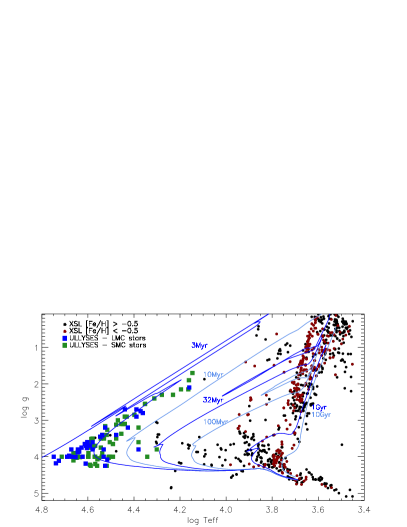
Figure 12: Comparison of the ULLYSES (blue: LMC; green: SMC) and XSL libraries. XSL stars (filled circles) are separated by metallicity: [Fe/H] $>-0.5$ (black) and [Fe/H] $<-0.5$ (dark red). Temperatures, gravities, and metallicities of the ULLYSES stars in this figure were obtained from the literature. Solid lines are Geneva isochrones for $Z_{\odot}$ and various ages (Ekström et al. 2012).

A.7 Population Synthesis (WG 7)

Population synthesis models are called semi-empirical if the stellar evolution tracks are theoretical but the individual stellar spectra are observed, and fully theoretical when both are calculated. XShootU observations will enable improvements of semi-empirical models because they will provide the most complete spectral library to date. In addition, the XShootU observations will guide new generations of atmosphere and evolution models, which will help improve fully theoretical population synthesis models. The new empirical library of LMC $+$ SMC UV-to-NIR massive-star spectra built by the ULLYSES and XShootU projects will replace the Starburst99 LMC $+$ SMC library, greatly improving the realism of population synthesis predictions. Once the library is implemented in Starburst99, corresponding Cloudy (Ferland et al. 2017) photoionization models will be computed in order to account for the contribution of the ionized gas and dust to the integrated light of young OB star populations. The models, which will be publicly available, will be used to interpret existing and future observations of star-forming and starburst galaxies with similar metallicities, in particular those from the COS Legacy Spectroscopic SurveY (CLASSY, Berg et al. 2022, James et al. 2022), which obtained the first high-resolution ($R\sim 15\,000$) FUV spectral database of 45 nearby ($0.002<z<0.182$) star-forming galaxies, the majority of which have LMC- or SMC-like metallicities.

A.8 Interstellar Medium (WG 8)

The intervening ISM along the line of sight to each target star will impact the observed UV and optical spectra. Cool atomic and molecular gas produces absorption features superimposed on stellar photospheric and wind lines. Furthermore, dust in the Milky Way and the host galaxy extinguishes and reddens the stellar spectra. These effects must be accounted for to reliably analyse stellar features, but also enable ISM science that is interesting in its own right. Due to the nature of the UV-based selection process of the target sample and the fact that most OB stars in the MCs experience low extinctions ($E(B-V)<0.20$ mag), strong ISM signatures are not expected in the optical and NIR X-shooter spectra. Nevertheless, clear signatures are expected in strong atomic lines such as the Na i $\lambda\lambda$5889.951,5895.924 and Ca ii $\lambda\lambda$3933.663,3968.468 doublets. For the targets with the strongest extinctions, detection are expected for some molecular lines, such as CH $\lambda$4300.313 and CH+ $\lambda$4232.548, and strong diffuse interstellar bands (DIBs), such as those at 4428 Å, 5780.5 Å, 5797.1 Å and 6614 Å. These lines have been well studied for Galactic targets but less so for objects in the MCs (though see, e.g., Ehrenfreund et al. 2002, Welty et al. 2006, Cox et al. 2006; 2007, van Loon et al. 2013, Bailey et al. 2015). The coverage of the significantly less studied wavelength region between $3200-3800$ Å could provide detections of some lines such as Ti i $\lambda$3729.8069 and Ti ii $\lambda$3383.759. In addition, the flux calibration of the X-shooter spectra will provide insights into the MC extinction laws (Maíz Apellániz et al. 2014) and possibly detect the recently discovered very broad absorption band centered on 7700 Å (Maíz Apellániz et al. 2021).

A.9 Massive Star Formation and Feedback (WG 9)

The energy output from young OB stars creates expanding H ii regions that are overpressurised with respect to their surroundings by photoionization, radiation pressure on dust grains, and shock heating by stellar winds (Mathews1967, Weaver1977, SpitzerLyman1978). Key stellar properties for the structure and dynamics of these regions are the flux in FUV and EUV photons and the stellar wind mass-loss rate and terminal velocity. The density distribution, chemistry, and equilibrium temperature of the photoionised gas also play important roles (Ferland2017). Because the LMC and SMC have substantially lower metallicities than the Galaxy, their H ii regions are ideal test cases for the impacts of stellar ionizing flux (Voges2008, Oey1997) and winds (e.g., Oey1996, Oey1998) in low-metallicity environments typical of high-redshift galaxies. The XShootU dataset in the Magellanic Clouds represents a significant opportunity to advance the state of the art in our understanding of how stars shape their environment. WG9 has identified a sample of relatively isolated XShootU stars that reside inside H ii regions identified in the mcels survey (Pellegrini2012). These single-star H ii regions are valuable tools for calibrating stellar atmosphere models (like those produced by WG 3) by comparing observed nebular emission lines to photoionization models adopting those model atmospheres as the ionizing sources (Zastrow2013). Combining stellar properties inferred from the XShootU spectra with the observed structure and emission of the ionized gas in these regions will clarify the role stars play in shaping their environment.

A.10 Stripped Stars (WG 10)

Stars stripped of their hydrogen-rich envelopes via mass transfer or common envelope ejection in binary systems are thought to be the fate of a third of all massive stars (Sana et al. 2012). In fact, in a continuously star-forming population, a few percent of all massive stars should be accompanied by a stripped companion. Binary-stripped stars are the exposed helium cores of their progenitors. During the long-lived phase of core helium burning these stars are small ($R_{\star}\lesssim 1\leavevmode\nobreak\ R_{\odot}$), hot ($T_{\rm eff}\sim 50-100$ kK), compact ($\log g\sim 5$), helium-rich ($Y_{\rm surf}\sim 0.5-1$), and hydrogen-poor ($X_{\rm surf}\sim 0-0.5$), but span a range of luminosities ($1-10^{6}\leavevmode\nobreak\ L_{\odot}$) and masses ($\sim 0.5-10\leavevmode\nobreak\ M_{\odot}$) (Götberg et al. 2018). After core-helium exhaustion, they can expand to giant sizes, depending on the fraction of hydrogen they retain, and appear as helium-enriched blue, yellow, or red supergiants (Yoon et al. 2017, Laplace et al. 2020). ULLYSES offers an excellent sample to search for hot binary-stripped stars that are sufficiently massive to explode as SNe. Especially with the effort to exclude apparent binaries from the target sample, the likelihood of having a few hidden binary-stripped companions increases, as they are not expected to significantly contribute to the optical flux or to cause large radial velocities. While UV spectra will be crucial for this analysis, the optical spectra are needed for stellar characterisation of both the binary-stripped star and the accretor star. We expect that discovering binary-stripped star $+$ OB star systems in the ULLYSES sample will help constrain uncertainties, such as how common and efficient mass transfer is, and exactly how the two stars are affected by such mass transfer.

A.11 Auxiliary/New Data (WG 11)

There are multiple ways in which auxiliary data can help to increase the value of the ULLYSES/XShootU library, including different wavelength regimes (e.g. X-rays) and observing strategies. For example, the intermediate spectral resolving power of the X-shooter data only partially resolves spectral lines, especially for stars with low projected rotational velocities ($v\sin i$), and higher resolution spectra are needed for a detailed spectroscopic analysis. WG 11 will provide high-resolution optical spectroscopy of a selection of slow rotating ULLYSES targets. Targets were selected on the basis of showing narrow, resolved C iii 1176 Å  lines in their UV spectra or having low $v\sin i$ reported in the literature. In Dec 2021 - Dec 2022, we obtained high resolution ($R\sim 40\,000$) and high signal-to-noise ratio (S/N $\sim 200$ in the 4100 Å  region) optical spectra with the 6.5m Magellan Clay telescope (+MIKE spectrograph) for 48 ULLYSES targets. Basic reductions confirmed the high quality of the data, and final reductions are underway. The Magellan/MIKE data will be made available to the massive stars community. WG11 also plans to organize archival searches aimed to identify data that will enhance the ULLYSES/XShootU library:

• High spectral resolution optical spectra of ULLYSES targets, e.g., obtained with the UVES, FLAMES, FEROS, and HARPS instruments.

• UV spectra obtained with IUE, FUSE, and HST.

A.12 Pulsations (WG 12)

The study of spectroscopic variability in XShootU targets is naturally supported by the analysis of time-series photometry from the NASA Transiting Exoplanet Survey Satellite (TESS) mission (Ricker et al. 2015). The LMC is within the southern continuous viewing zone of the TESS mission, such that all XShootU stars in the LMC have continuous light curves spanning 1 yr. TESS light curves have been used to demonstrate that heat-driven pulsations and the signatures of rotational modulation are common in early-type main-sequence stars in the Galaxy (David-Uraz et al. 2019, Burssens et al. 2020). Whereas, the brightest massive stars in the MCs, i.e., OB supergiants, have light curves dominated by stochastic low-frequency variability (SLF; Bowman et al. 2019). Interestingly, in low metallicity environments such as the MCs, the driving of heat-driven pulsations is less efficient (Salmon et al. 2012). For massive stars with identified pulsation modes, forward asteroseismic modelling is able to provide constraints on their (core) masses, ages, interior rotation profiles, and mixing properties (e.g. Aerts et al. 2003, Dupret et al. 2004, Salmon et al. 2021), but also probe the strength and geometry of an interior magnetic field (Lecoanet et al. 2022). A key goal of WG12 is to extract reliable TESS light curves, provide complementary constraints on the variability amplitudes and timescales of each XShootU target, and ultimately perform forward asteroseismic modelling (see Bowman 2020 for a review).

A.13 Magnetic Fields (WG13)

WG13 seeks to leverage the UV and optical spectral libraries provided by the ULLYSES and XShootU programmes to shed light on how magnetism affects massive star structure and evolution. In magnetic massive stars, which make up $\sim$7% of the total OB star population (e.g., Morel et al. 2015, Wade et al. 2016, Grunhut et al. 2017), stable, nearly dipolar surface magnetic fields warp the stellar wind into a structurally complex magnetosphere, trapping the wind near the stellar surface, thus significantly altering the circumstellar environment. This magnetic wind confinement has been shown to reduce stellar mass-loss rate compared to non-magnetic stars of similar spectral type (ud-Doula et al. 2008). It should be noted that atypical features in P-Cygni profiles are not necessarily the result of a magnetic fields, as variability in the absorption components of wind-sensitive UV resonance lines have also been observed in non-magnetic massive stars (e.g., Massa et al. 1995, Kaper et al. 1996; 1999). Erba et al. (2021)’s synthetic line profiles can be adapted for direct comparison with observations, and used in conjunction with the XShootU spectral libraries to identify new magnetic candidates.

A.14 Unusual Objects (WG14)

Finally, the data offer many opportunities to study key objects. For example, combining the radial velocities from XShootU with the exquisite proper motions from Gaia DR3, we can reconstruct the space motions of ULLYSES targets, which can be used to identify runaway and walkaway stars. Moreover, Gaia DR3 light-curves can be used in conjunction with radial velocities of known eclipsing binaries to estimate fundamental stellar parameters, providing unique tests of stellar evolution.

Appendix B ULLYSES target parameters

In this Appendix we present a literature search for the stellar and wind parameters as they were known prior to the start of ULLYSES. Obviously, these data (see Table A1) are rather heterogeneous and they will quickly become outdated as new spectral analyses are underway.

Table 4: Pre-ULLYSES target parameters compiled by the ULLYSES team at STScI. References have been added in columns for all parameters.

Target	SpType	Ref	$T_{\mathrm{eff}}$	Ref	$\log\leavevmode\nobreak\ g$	Ref	$\log\leavevmode\nobreak\ L/L_{\odot}$	Ref	$R/R_{\odot}$	Ref	$M/M_{\odot}$	Ref	$v\sin i$	Ref	$v_{\mathrm{inf}}$	Ref	$\dot{M}$	Ref
			(K)		(cgs)								(km s-1)		(km s-1)		($M_{\odot}\leavevmode\nobreak\$yr-1)
SMC targets
2dFS 163	O8 Ib(f)	1	-	-	-	-	-	-	-	-	-	-	-	-	-	-	-	-
AzV 6	O9 III	2	-	-	-	-	-	-	-	-	-	-	-	-	-	-	-	-
AzV 14	O5 V	3	44000	3	4.0	3	5.82	3	14.2	3	74.0	3	261	4	2000	3	1.0E-07	3
AzV 15	O6.5 II(f)	5	39000	6	3.6	6	5.83	6	18.0	From L,Teff	47.2	6	120	6	2050	6	1.1E-06	6
AzV 16	sgB0[e—	7	-	-	-	-	-	-	-	-	-	-	-	-	-	-	-	-
AzV 18	B2 Ia	2	19000	8	2.3	8	5.44	8	49.0	8	28.0	8	49	8	325	9	2.3E-07	8
AzV 22	B5 Ia	2	14500	8	1.9	8	5.04	8	53.0	8	19.0	8	46	8	280	8	2.3E-07	8
AzV 39a	WN5ha	10	47000	11	-	-	5.57	11	9.1	11	43.0	11	-	-	900	11	1.8E-06	11
AzV 43	B0.5 III	12	28500	6	3.4	6	5.13	6	15.1	From L,Teff	22.4	6	200	6	1200	6	2.2E-08	6
AzV 47	O8 III((f))	5	35000	6	3.8	6	5.44	6	14.3	6	42.2	6	60	6	2000	6	2.1E-08	6
AzV 61	O6 III((f))e	13	-	-	-	-	-	-	-	-	-	-	228	4	2025	14	-	-
AzV 69	OC7.5 III((f))	5	33900	6	3.5	6	5.61	6	18.6	From L,Teff	39.7	6	70	6	1800	6	9.8E-07	6
AzV 70	O9.5 Ibw	15	28500	16	3.1	16	5.68	16	28.4	16	-	-	100	16	1450	16	1.5E-06	16
AzV 75	O5 III(f+)	5	38500	6	3.5	6	5.94	6	21.0	From L,Teff	51.1	6	120	6	2050	6	1.6E-06	6
AzV 81	WN6h	10	45000	11	-	-	5.78	11	13.0	11	38.0	11	-	-	1000	11	6.6E-06	11
AzV 80	O4-6n(f)p	5	38000	17	3.5	17	-	-	-	-	-	-	325	17	1550	9	-	-
AzV 83	O7 Iaf+	5	32800	6	3.3	6	5.54	6	18.3	From L,Teff	22.1	6	80	6	940	6	2.3E-06	6
AzV 85	B1 II-IIIe	18	-	-	-	-	-	-	-	-	-	-	-	-	-	-	-	-
AzV 95	O7 III((f))	5	38200	19	3.7	19	5.56	19	13.8	19	39.3	19	68	19	1700	9	3.6E-07	19
AzV 96	B1.5 Ia	2	22000	20	2.6	20	5.39	20	34.0	20	27.0	20	90	20	850	20	2.4E-07	20
AzV 104	B0.5 Ia	2	27500	8	3.1	8	5.31	8	20.0	8	26.0	8	80	8	1340	8	4.0E-07	8
AzV 148	O8.5 V	21	32300	22	4.0	22	4.84	22	8.4	From L,Teff	19.0	22	60	22	1540	22	2.0E-09	22
2dFS 999	WN3 ha	10	100000	11	-	-	6.05	11	3.5	11	-	-	-	-	1800	11	2.2E-06	11
NGC330 ELS 4	B2.5 Ib	23	17000	24	2.3	24	4.77	24	28.0	From L,Teff	15.0	24	41	24	-	-	-	-
NGC330 ELS 2	B3 Ib	23	14590	24	2.2	24	4.73	24	36.3	From L,Teff	15.0	24	14	24	-	-	-	-
AzV 175	B1 IIW	25	-	-	-	-	-	-	-	-	-	-	51	4	-	-	-	-
AzV 177	O4 V((f))	26	44500	22	4.0	22	5.43	22	8.7	From L,Teff	38.8	22	220	22	2400	22	1.4E-07	22
AzV 186	O8.5 III((f))	13	34500	19	3.4	19	5.40	19	14.1	19	32.2	19	73	19	1600	19	3.0E-07	19
AzV 187	B3 Ia	2	-	-	-	-	-	-	-	-	-	-	-	-	-	-	-	-
AzV 189	O9 V	21	32300	22	4.0	22	4.81	22	8.1	From L,Teff	18.8	22	150	22	1250	22	6.0E-10	22
AzV 200	B8 Ia	2	12100	27	1.7	27	-	-	-	-	-	-	-	-	-	-	-	-
NGC346 ELS 43	B0 V	23	33000	28	4.3	28	4.71	28	6.9	From L,Teff	18.0	28	10	28	-	-	-	-
NGC346 ELS 26	O9.5-B0 V (N str)	5	31000	22	3.7	22	4.93	22	10.1	From L,Teff	21.0	22	60	22	1250	22	5.0E-10	22
NGC346 ELS 28	OC6 Vz	5	39600	22	4.0	22	5.15	22	8.0	From L,Teff	27.8	22	35	22	1250	22	3.0E-09	22
AzV 207	O7 III((f))	13	37000	3	3.7	3	5.34	3	11.0	3	22.0	3	75	4	-	-	-	-
AzV 210	B1.5 Ia	2	20500	8	2.4	8	5.41	8	40.0	8	27.0	8	65	8	750	9	2.0E-07	8
NGC346 ELS 50	O8 Vn	23	36300	22	4.3	22	4.64	22	5.3	From L,Teff	19.5	22	360	22	1540	22	3.0E-09	22
AzV 215	BN0 Ia	2	27000	8	2.9	8	5.63	8	30.0	8	39.0	8	91	8	1400	9	1.4E-06	8
NGC346 ELS 7	O4 V((f))	29	42100	22	4.0	22	5.51	22	10.7	From L,Teff	40.0	22	70	22	2300	22	1.4E-07	22
NGC346 MPG 355	ON2 III(f*)	30	51700	22	4.0	22	6.04	22	13.1	From L,Teff	70.0	22	120	22	2800	22	1.8E-07	22
NGC346 MPG 368	O6 V	31	39300	22	3.8	22	5.38	22	10.6	From L,Teff	33.2	22	60	22	2100	22	3.7E-08	22
NGC346 MPG 435	O4 If	32	-	-	-	-	-	-	-	-	-	-	93	4	-	-	-	-
NGC346 ELS 51	O7 Vz	23	38700	22	4.3	22	4.80	22	5.6	From L,Teff	23.1	22	50	22	1950	22	6.0E-10	22
AzV 224	B1 III	25	-	-	-	-	-	-	-	-	-	-	299	33	-	-	-	-
HD 5980	WN6h	10	43000	34	3.5	34	6.35	34	24.0	34	61.0	34	-	-	2200	34	3.2E-05	34
NGC346 ELS 13	O9 V	35	34500	35	3.9	35	-	-	-	-	-	-	320	35	-	-	-	-
NGC346 ELS 46	O7 Vn	23	39000	22	4.2	22	4.81	22	5.6	From L,Teff	23.7	22	300	22	1950	22	6.0E-10	22
AzV 232	O7 Iaf+	36	33500	6	3.2	6	5.89	6	26.2	From L,Teff	35.3	6	75	6	1350	6	4.5E-06	6
AzV 234	B3 Iab	32	15700	32	2.2	32	4.91	32	38.6	From L,Teff	-	-	43	32	-	-	-	-
AzV 235	B0 Iaw	37	27500	16	2.9	16	5.72	16	31.9	16	-	-	80	16	1400	16	4.0E-06	16
NGC346 ELS 35	B1 V	23	-	-	-	-	-	-	-	-	-	-	145	33	-	-	-	-
NGC346 ELS 25	O9 V	23	36200	19	4.1	19	4.90	19	7.2	19	22.6	19	138	19	2816	19	1.3E-07	19
NGC346 ELS 31	O8 Vz	23	37200	22	4.0	22	4.95	22	7.2	From L,Teff	23.2	22	25	22	1540	22	6.0E-10	22
AzV 238	O9.5 III	5	-	-	-	-	-	-	-	-	-	-	71	4	1200	38	-	-
AzV 243	O6 V	29	39600	22	3.9	22	5.59	22	13.3	From L,Teff	41.0	22	60	22	2000	22	7.9E-08	22
AzV 242	B0.7 Iaw	37	25000	20	2.9	20	5.67	20	36.6	20	39.5	20	83	4	950	9	8.4E-07	20
AzV 251	O7.5 V	13	33100	39	-	-	4.89	39	8.5	From L,Teff	-	-	-	-	-	-	-	-
AzV 255	O8 V	21	-	-	-	-	-	-	-	-	-	-	188	4	-	-	-	-
AzV 261	B2 Ibe	1	-	-	-	-	-	-	-	-	-	-	87	4	-	-	-	-
AzV 264	B1 Ia	2	22500	20	2.6	20	5.44	20	34.8	20	29.0	20	85	20	600	9	2.9E-07	20
AzV 266	B1 I	13	18200	39	-	-	5.09	39	35.3	From L,Teff	-	-	61	4	-	-	-	-
AzV 267	O8 V	13	35700	22	4.0	22	4.90	22	7.4	From L,Teff	21.5	22	220	22	1250	22	2.5E-09	22
AzV 296	O7.5 V((f))	3	35000	3	3.5	3	5.30	3	11.9	3	16.0	3	-	-	2000	3	5.0E-07	3
AzV 304	B0.5 V	40	27500	41	3.9	41	-	-	-	-	-	-	11	42	-	-	-	-
AzV 307	O9 III	25	30000	6	3.5	6	5.15	6	13.9	From L,Teff	22.5	6	60	6	1300	6	4.8E-09	6
AzV 314	B5 Iab	2	-	-	-	-	-	-	-	-	-	-	-	-	-	-	-	-
AzV 321	O9 IInp	43	-	-	-	-	-	-	-	-	-	-	357	4	-	-	-	-
AzV 324	B4 Iab	44	-	-	-	-	-	-	-	-	-	-	-	-	-	-	-	-
AzV 326	O9 V	21	32400	22	4.0	22	4.81	22	8.1	From L,Teff	18.8	22	200	22	1250	22	7.1E-10	22
AzV 327	O9.5 II-Ibw	5	30000	6	3.1	6	5.54	6	21.8	From L,Teff	22.8	6	95	6	1500	6	1.3E-07	6
AzV 332	WN3:h	45	80000	45	-	-	5.87	45	4.7	45	-	-	-	-	2000	45	6.3E-06	45
AzV 343	B6 Iab	44	-	-	-	-	-	-	-	-	-	-	-	-	-	-	-	-
AzV 362	B3 Ia	2	14000	8	1.7	8	5.50	8	96.0	8	30.0	8	51	8	270	8	8.0E-07	8
AzV 372	O9.5 Iabw	15	28000	16	3.1	16	5.62	16	27.5	16	-	-	120	16	1550	16	1.0E-06	16
AzV 374	B2 Ib	2	18500	46	2.5	46	-	-	-	-	-	-	47	47	-	-	-	-
AzV 377	O5 V((f))	1	45500	3	4.0	3	5.54	3	9.1	3	45.0	26	-	-	2350	3	1.0E-07	3
AzV 388	O4 V	25	43100	22	4.0	22	5.54	22	10.6	From L,Teff	42.0	22	150	22	2100	22	1.0E-07	22
AzV 393	B1.5 Ia	25	-	-	-	-	-	-	-	-	-	-	-	-	-	-	-	-
AzV 410	B0 III	25	-	-	-	-	-	-	-	-	-	-	-	-	-	-	-	-
2dFS 2266	OC7 II(f)	1	-	-	-	-	-	-	-	-	-	-	-	-	-	-	-	-
AzV 423	O9.5 II(n)	15	28200	39	-	-	5.34	39	19.6	From L,Teff	-	-	163	4	-	-	-	-
AzV 435	O3 V((f*))	26	46000	48	3.9	48	5.88	48	13.8	48	-	-	110	48	1500	48	2.1E-07	48
AzV 440	O8 V	26	37000	26	4.0	26	5.28	26	10.6	26	42.0	26	62	4	1300	26	1.0E-07	26
AzV 445	B5 Iab	2	-	-	-	-	-	-	-	-	-	-	-	-	-	-	-	-
2dFS 2553	O6.5 III((f))e	13	-	-	-	-	-	-	-	-	-	-	-	-	-	-	-	-
AzV 446	O6.5 V	25	39700	22	4.0	22	5.25	22	8.9	From L,Teff	30.0	22	30	22	1400	22	4.0E-09	26
AzV 456	O9.5 Ibw	16	29500	16	3.0	16	5.81	16	30.6	16	-	-	80	16	1450	16	7.0E-07	16
AzV 468	O8.5 V	25	34700	22	4.0	22	4.76	22	6.6	From L,Teff	19.3	22	50	22	1540	22	7.1E-10	22
AzV 469	O8.5 II((f))	15	33000	16	3.4	16	5.50	16	17.2	16	-	-	80	16	1550	16	1.3E-06	16
AzV 472	B2 Ia	2	19000	46	2.4	46	-	-	-	-	-	-	33	47	-	-	-	-
AzV 476	O2-3 V	26	40000	39	-	-	5.71	39	14.9	From L,Teff	-	-	65	4	2670	26	-	-
AzV 479	O9 Ib	2	-	-	-	-	-	-	-	-	-	-	-	-	-	-	-	-
AzV 488	B0.5 Iaw	37	27500	16	2.9	16	5.74	16	32.6	16	-	-	80	16	1250	16	1.2E-06	16
AzV 490	B0 Iwp var	37	-	-	-	-	-	-	-	-	-	-	-	-	-	-	-	-
AzV 506	B0.5 II	13	25700	39	-	-	5.10	39	17.9	From L,Teff	-	-	-	-	-	-	-	-
$[$M2002$]$ SMC 81469	O9.7 V	49	31000	49	4.0	49	4.90	49	9.8	49	35.0	49	70	49	2100	49	4.0E-09	49
2dFS 3689	B1.5 V	49	22000	49	4.0	49	4.30	49	9.8	49	9.3	50	250	49	900	49	2.0E-09	49
2dFS 3694	B1 IV	49	24000	49	3.6	49	4.69	49	12.8	49	24.0	49	120	49	1600	49	2.5E-09	49
SK 173	B0.7 IIe	49	24000	49	3.2	49	5.00	49	18.3	49	19.0	49	120	49	1100	49	5.0E-09	49
2dFS 3780	O9.7 IV	49	32000	49	4.0	49	4.85	49	8.7	49	28.0	49	30	49	1900	49	3.2E-09	49
SK 179	B6 I	51	-	-	-	-	-	-	-	-	-	-	-	-	-	-	-	-
SK 183	O3 V((f*))z	49	46000	49	4.1	49	5.61	49	10.1	49	47.0	49	100	49	2900	49	3.2E-08	49
2dFS 3947	B1.5 IV	49	20000	49	3.8	49	4.33	49	12.2	49	34.0	49	140	49	752	49	7.9E-10	49
2dFS 3954	O6 V((f))z	49	37000	49	4.2	49	4.75	49	5.8	49	19.0	49	40	49	2500	49	2.5E-09	49
SK 187	O8.5 III	49	32000	49	3.6	49	5.40	49	16.4	49	39.0	49	100	49	1900	49	1.3E-08	49
SK 191	B1.5 Ia	2	22500	8	2.6	8	5.77	8	51.0	8	41.0	8	96	8	425	9	6.8E-07	8
LMC targets
SK -67 2	B1 Ia+ (N wk)	52	19910	53	2.3	53	-	-	-	-	-	-	-	-	-	-	-	-
SK -67 5	O9.7 Ib	36	-	-	-	-	-	-	-	-	-	-	90	54	-	-	-	-
BI 13	O6.5 V	55	-	-	-	-	-	-	-	-	-	-	118	4	-	-	-	-
SK -68 8	B5 Ia+	56	-	-	-	-	-	-	-	-	-	-	-	-	-	-	-	-
SK -70 13	O9 V	21	-	-	-	-	-	-	-	-	-	-	84	4	-	-	-	-
SK -67 14	B1.5 Ia	15	22890	53	2.7	53	-	-	-	-	-	-	88	4	-	-	-	-
SK -70 16	B4 I	57	-	-	-	-	-	-	-	-	-	-	-	-	-	-	-	-
SK -67 20	WN4 b	58	158000	59	-	-	5.84	59	1.1	59	25.0	59	-	-	1600	59	3.3E-05	59
SK -66 17	OC9.5 II	23	29500	33	3.2	33	5.49	33	-	-	35.0	33	60	33	-	-	-	-
SK -66 18	O6 V((f))	21	40200	60	3.8	60	5.55	60	12.2	60	40.7	60	82	60	2200	60	1.1E-06	60
SK -69 43	B0.5 Ia	56	22845	53	2.6	53	-	-	-	-	-	-	102	4	-	-	-	-
N11 ELS 33	B0 IIIn	23	26700	61	3.2	61	5.05	61	15.7	61	-	-	256	61	1540	61	2.5E-07	61
N11 ELS 49	O7.5 V	23	-	-	-	-	-	-	-	-	-	-	-	-	-	-	-	-
N11 ELS 51	O5 Vn((f))	23	41400	61	3.7	61	5.42	61	8.6	61	-	-	350	61	2110	61	4.1E-07	61
N11 ELS 18	O6 II(f+)	23	-	-	-	-	-	-	-	-	-	-	110	4	-	-	-	-
N11 ELS 60	O3 V((f*))	62	48000	61	4.0	61	5.63	61	9.5	61	-	-	68	61	2740	61	5.1E-07	61
N11 ELS 31	ON2 III(f*)	30	56000	48	4.0	48	6.12	48	12.2	48	-	-	71	48	3200	14	2.2E-06	48
PGMW 3070	O6 V	63	-	-	-	-	-	-	-	-	-	-	72	4	-	-	-	-
N11 ELS 46	O9.5 V	23	33500	33	4.3	33	5.21	33	-	-	28.0	33	205	33	-	-	-	-
N11 ELS 38	O5 III(f+)	23	40500	61	3.7	61	5.67	61	14.0	61	-	-	100	61	2600	61	1.2E-06	61
PGMW 1363	O8.5 Iaf	63	-	-	-	-	-	-	-	-	-	-	-	-	-	-	-	-
PGMW 3120	O5.5 V((f*))	63	-	-	-	-	-	-	-	-	-	-	111	4	-	-	-	-
LMCe055-1	WN4 /O4	64	-	-	-	-	-	-	-	-	-	-	-	-	-	-	-	-
N11 ELS 20	O5 Inf+p	43	-	-	-	-	-	-	-	-	-	-	260	43	-	-	-	-
SK -65 2	B1 V	21	-	-	-	-	-	-	-	-	-	-	-	-	-	-	-	-
N11 ELS 26	O2.5 III(f*)	23	49000	48	4.0	48	5.82	48	11.3	48	-	-	72	48	3120	48	1.6E-06	48
N11 ELS 32	O7 II(f)	23	36000	61	3.5	61	5.44	61	13.6	61	-	-	60	61	1920	61	9.7E-07	61
N11 ELS 48	O6.5 V((f))	23	40700	60	4.2	60	5.38	60	9.9	60	36.6	60	130	60	3790	60	1.7E-07	60
N11 ELS 13	O8 V	23	-	-	-	-	-	-	-	-	-	-	147	4	-	-	-	-
SK -66 35	BC1 Ia	52	22000	53	2.6	53	-	-	-	-	-	-	-	-	-	-	-	-
SK -69 50	O7(n)(f)p	43	-	-	-	-	-	-	-	-	-	-	210	43	-	-	-	-
SK -68 15	WC4	65	90000	66	-	-	5.70	66	2.9	66	-	-	-	-	3000	66	3.2E-05	66
SK -67 22	O2 If*/WN5	67	50000	59	-	-	5.80	59	10.6	59	53.0	59	200	48	2400	59	5.0E-06	59
SK -68 16	O7 III	65	-	-	-	-	-	-	-	-	-	-	100	4	-	-	-	-
SK -69 52	B2 Ia	56	-	-	-	-	-	-	-	-	-	-	105	4	-	-	-	-
SK -70 32	O9.5 II:	56	-	-	-	-	-	-	-	-	-	-	97	4	-	-	-	-
SK -68 23a	B1 III	21	-	-	-	-	-	-	-	-	-	-	-	-	-	-	-	-
SK -65 22	O6 Iaf+	36	33500	68	3.2	68	5.86	68	25.0	68	-	-	90	68	1520	68	1.1E-05	68
SK -68 26	BC2 Ia	52	18160	53	2.2	53	-	-	-	-	-	-	-	-	-	-	-	-
SK -66 50	B8 Ia+	52	11900	53	1.5	53	-	-	-	-	-	-	-	-	-	-	-	-
SK -70 50	B3 Ia	52	-	-	-	-	-	-	-	-	-	-	-	-	-	-	-	-
SK -70 60	O4-5 V((f))pec	31	-	-	-	-	-	-	-	-	-	-	256	4	2150	14	-	-
SK -70 69	O5.5 V((f))	31	40500	31	3.7	31	5.35	31	9.6	31	-	-	98	4	2300	31	8.0E-07	31
SK -68 41	B0.5 Ia	56	24500	31	2.9	31	5.56	31	33.4	31	33.0	31	77	4	865	14	9.0E-07	31
SK -70 79	B0 III	21	-	-	-	-	-	-	-	-	-	-	86	4	-	-	-	-
SK -68 52	B0 Ia	36	24500	16	2.7	16	5.76	16	42.2	16	-	-	80	16	1400	16	3.2E-06	16
SK -71 8	O9 II	69	-	-	-	-	-	-	-	-	-	-	75	4	-	-	-	-
HV 5622	B0 V	70	-	-	-	-	-	-	-	-	-	-	-	-	-	-	-	-
SK -67 51	O6.5 III	69	-	-	-	-	-	-	-	-	-	-	-	-	-	-	-	-
SK -67 69	O4 III(f)	71	-	-	-	-	-	-	-	-	-	-	121	4	2500	72	-	-
SK -69 83	O7.5 Iaf	56	-	-	-	-	-	-	-	-	-	-	-	-	-	-	-	-
BI 128	O9 V	21	-	-	-	-	-	-	-	-	-	-	-	-	-	-	-	-
SK -69 104	O6 Ib(f)	36	-	-	-	-	-	-	-	-	-	-	117	4	2160	14	-	-
SK -67 78	B3 Ia	52	16150	53	2.0	53	-	-	-	-	-	-	-	-	-	-	-	-
SK -65 47	O4 I(n)f+p	43	40500	48	3.6	48	5.98	48	19.8	48	-	-	160	48	2100	48	1.1E-05	48
SK -65 55	WN6 h	73	47000	59	-	-	5.65	59	10.0	59	-	-	-	-	1000	59	8.9E-06	59
SK -71 19	O6 III	69	-	-	-	-	-	-	-	-	-	-	242	4	-	-	-	-
SK -71 21	WN6(h)	74	47000	59	-	-	5.94	59	13.9	59	-	-	-	-	1600	59	2.3E-05	59
SK -68 73	WN9pec	75	28000	59	-	-	6.50	59	74.8	59	-	-	-	-	400	59	3.7E-05	59
SK -67 101	O8 II((f))	15	-	-	-	-	-	-	-	-	-	-	103	4	2005	14	-	-
SK -67 105	O4 f + O6 V	76	-	-	3.6	76	-	-	16.9	76	48.3	76	-	-	-	-	-	-
SK -67 106	O8 III((f))	77	-	-	-	-	-	-	-	-	-	-	99	4	-	-	-	-
SK -67 107	O9 Ib(f)	77	-	-	-	-	-	-	-	-	-	-	82	4	-	-	-	-
SK -67 108	O4-5 III	56	-	-	-	-	-	-	-	-	-	-	-	-	-	-	-	-
LH 58-496	O5 V((f))	65	42000	26	4.0	26	5.48	26	10.5	26	44.0	26	-	-	2400	26	6.0E-07	26
SK -67 111	O6 Ia(n)fpv	43	-	-	-	-	-	-	-	-	-	-	230	43	2000	72	-	-
BI 173	O8 II:	15	34500	31	3.4	31	5.60	31	17.6	31	40.0	31	200	31	1950	14	1.6E-06	31
SK -67 118	O7 V	21	-	-	-	-	-	-	-	-	-	-	61	4	-	-	-	-
SK -69 140	B4 I	57	-	-	-	-	-	-	-	-	-	-	-	-	-	-	-	-
SK -66 100	O6 II(f)	29	39000	61	3.7	61	5.59	61	13.7	61	-	-	59	61	2075	61	8.3E-07	61
SK -71 35	B1 II	78	23000	78	2.8	78	5.34	78	29.5	78	20.0	78	87	78	400	78	1.1E-06	78
BI 184	O8 (V)e	78	34000	78	4.0	78	5.28	78	12.6	78	58.0	78	100	78	2470	78	2.2E-07	78
SK -71 41	O9.7 Iab	78	30000	78	3.4	78	5.50	78	20.9	78	40.0	78	90	78	1800	78	8.1E-07	78
NGC2004 ELS 3	B5 Ia	23	14450	24	2.1	24	5.10	24	56.7	From L,Teff	20.0	24	42	24	-	-	-	-
BI 189	O8 IV((f))e	79	34000	79	3.8	79	5.60	79	18.2	79	77.0	79	83	79	2100	79	9.3E-07	79
N206-FS 170	B1 IV	78	24000	78	3.8	78	4.55	78	10.9	78	28.0	78	80	78	2100	78	2.0E-08	78
SK -71 45	O4-5 III(f)	36	38000	79	3.6	79	6.28	79	31.9	79	148.0	79	116	79	2300	79	1.6E-05	79
SK -67 166	O4 If+	36	40000	68	3.6	68	5.98	68	20.5	68	-	-	97	4	1750	68	8.5E-06	68
SK -71 46	O4 If	21	38000	79	3.6	79	6.10	79	26.0	79	98.0	79	98	79	2300	79	1.2E-05	79
SK -67 167	O4 Inf+	71	-	-	-	-	-	-	-	-	-	-	155	4	2200	72	-	-
SK -67 168	O8 I(f)p	43	-	-	-	-	-	-	-	-	-	-	-	-	-	-	-	-
SK -69 178	O9.2 II	80	-	-	-	-	-	-	-	-	-	-	-	-	-	-	-	-
LMC X-4	O8 III	81	-	-	-	-	-	-	-	-	-	-	-	-	-	-	-	-
SK -67 191	O8 V	69	-	-	-	-	-	-	-	-	-	-	100	4	1950	72	-	-
SK -67 195	B6 I	57	-	-	-	-	-	-	-	-	-	-	-	-	-	-	-	-
SK -67 197	B7 I	57	-	-	-	-	-	-	-	-	-	-	-	-	-	-	-	-
SK -66 152	O7 Ib(f)	56	-	-	-	-	-	-	-	-	-	-	-	-	-	-	-	-
SK -69 191	WC4	65	85000	66	-	-	5.68	66	3.2	66	-	-	-	-	3200	66	4.0E-05	66
W61 28-5	O4 V((f+))	3	44000	48	3.8	48	5.51	48	9.8	48	-	-	120	48	2700	48	1.1E-06	48
W61 28-23	O3.5 V((f+))	26	47000	48	3.8	48	5.65	48	10.0	48	-	-	146	48	3050	48	1.6E-06	48
SK -67 207	B9 Ia	56	-	-	-	-	-	-	-	-	-	-	-	-	-	-	-	-
SK -67 211	O2 III(f*)	62	52500	30	-	-	6.34	30	17.9	From L,Teff	-	-	-	-	3750	29	2.5E-06	30
MCPS 083.91120-69.69685	O3 If*	80	-	-	-	-	-	-	-	-	-	-	-	-	-	-	-	-
SK -67 216	B0.5 V0	21	-	-	-	-	-	-	-	-	-	-	-	-	-	-	-	-
SK -69 212	O5n(f)p	43	-	-	-	-	-	-	-	-	-	-	-	-	-	-	-	-
BI 237	O2 V((f*))	26	53200	48	4.1	48	5.83	48	9.7	48	-	-	140	48	3400	48	6.2E-07	48
SK -68 133	OC3.5 III(f*)	80	-	-	-	-	-	-	-	-	-	-	-	-	-	-	-	-
SK -66 171	O9 Ia	56	-	-	-	-	-	-	-	-	-	-	90	4	-	-	-	-
LMCe078-1	O6 Ifc	64	-	-	-	-	-	-	-	-	-	-	-	-	-	-	-	-
VFTS 66	O9 V	82	32800	82	4.1	82	4.54	82	5.8	82	16.6	82	117	82	-	-	-	-
VFTS 72	O2 V-III(n)((f*))	83	54800	48	4.2	48	5.97	48	10.7	48	-	-	230	48	3180	26	1.5E-06	48
SK -68 135	ON9.7 Ia+	36	27500	16	2.7	16	5.97	16	42.3	16	-	-	70	16	1350	16	7.5E-06	16
VFTS 169	O2.5 V(n)((f*))	83	47300	84	-	-	5.89	84	13.1	From L,Teff	76.0	84	200	84	3200	84	3.2E-06	84
VFTS 180	O3 If*	67	42200	84	-	-	5.92	84	17.1	From L,Teff	58.0	84	93	84	2500	84	1.0E-05	84
VFTS 190	O7 Vnn((f))p	83	-	-	-	-	-	-	-	-	-	-	445	85	-	-	-	-
VFTS 244	O5 III(n)(fc)	83	41050	86	3.7	86	5.58	86	12.4	86	39.2	86	230	86	2123	86	2.2E-06	86
VFTS 267	O3 III-I(n)f*	83	44100	86	3.9	86	5.96	86	16.6	86	65.6	86	182	86	3208	86	1.0E-05	86
SK -68 137	O2 III(f*)	30	55000	30	-	-	6.19	30	13.7	From L,Teff	-	-	107	4	3200	14	2.0E-06	30
VFTS 355	O4 V((n))((fc))z	83	43400	87	3.8	87	5.52	87	10.4	87	57.3	87	134	88	-	-	-	-
VFTS 404	O3.5 V(n)((fc))	83	44700	84	-	-	5.91	84	-	-	78.0	84	-	-	3010	84	1.6E-06	84
VFTS 406	O6 Vnn	83	37600	84	-	-	5.48	84	13.0	From L,Teff	44.0	84	356	88	2600	84	4.0E-06	84
VFTS 482	O2.5 If*/WN6	67	42200	84	-	-	6.40	84	29.7	From L,Teff	145.0	84	200	84	2600	84	4.0E-05	84
VFTS 506	ON2 V((n))((f*))	83	47300	84	-	-	6.24	84	19.7	From L,Teff	122.0	84	93	88	3040	84	2.5E-06	84
BAT99 105	O2 If*	67	47300	84	-	-	6.56	84	28.4	From L,Teff	189.0	84	200	84	2800	84	2.5E-05	84
VFTS 542	O2 If*/WN5	89	47000	89	-	-	6.14	89	18.0	89	101.0	89	130	89	1800	89	1.0E-05	89
VFTS 545	O2 If*/WN5	67	47300	84	-	-	6.30	84	21.1	From L,Teff	133.0	84	200	84	2800	84	2.5E-05	84
VFTS 586	O4 V((n))((fc))z	83	45000	90	4.0	90	5.42	90	8.5	From L,Teff	-	-	100	90	-	-	-	-
SK -68 140	B0.7 Ib-Iab Nwk	91	23500	92	2.8	92	5.64	92	39.9	From L,Teff	37.0	92	53	92	-	-	-	-
HD 269927C	WN9h	58	32000	59	-	-	5.58	59	20.6	59	32.0	59	-	-	500	59	4.7E-06	59
$[$ST92$]$ 5-52	O3V ((f*))	62	-	-	-	-	-	-	-	-	-	-	-	-	3100	26	-	-
$[$ST92$]$ 5-27	O3 V((f))	65	47000	48	4.0	48	5.46	48	8.1	48	-	-	120	48	2400	48	2.7E-07	48
$[$ST92$]$ 4-18	O5 If	65	-	-	-	-	-	-	-	-	-	-	-	-	-	-	-	-
BI 265	O5 III(fc)	80	-	-	-	-	-	-	-	-	-	-	280	43	-	-	-	-
Farina 88	O4 III(f)	93	-	-	-	-	-	-	-	-	-	-	-	-	-	-	-	-
SK -71 50	O6.5 III	69	-	-	-	-	-	-	-	-	-	-	296	4	-	-	-	-
SK -69 279	O9.2 Iaf	94	29500	94	-	-	5.54	94	22.7	94	-	-	97	94	800	94	5.5E-06	94
SK -68 155	B0.5 I	57	-	-	-	-	-	-	-	-	-	-	96	4	-	-	-	-
LH 114-7	O2 III(f*)	62	-	-	-	-	-	-	-	-	-	-	-	-	3200	26	-	-
BI 272	O7 II	69	-	-	-	-	-	-	-	-	-	-	212	4	3400	72	-	-
SK -67 261	O8.5 III	21	-	-	-	-	-	-	-	-	-	-	-	-	-	-	-	-
SK -67 266	WN11h	74	28000	59	-	-	5.69	59	29.4	59	41.0	59	-	-	200	59	3.8E-06	59
SK -70 115	O6 If	95	-	-	-	-	-	-	-	-	-	-	164	4	2200	72	-	-
NGC 3109 targets
NGC 3109 EBU 07	B0-1 Ia	96	27000	96	2.9	96	5.82	96	37.0	96	39.7	96	-	-	-	-	-	-
NGC 3109 EBU 20	O8 I	96	31150	97	3.5	97	5.87	97	23.7	97	69.1	97	110	97	2166	97	4.5E-06	97
NGC 3109 EBU 34	O8 I(f)	96	33050	97	3.2	97	5.69	97	21.8	97	25.0	97	82	97	1357	97	1.8E-06	97
Sextans A targets
Sextans A GHF s4	O6 Vz	98	-	-	-	-	-	-	-	-	-	-	-	-	-	-	-	-
Sextans A GHF s2	O3-5 Vz	98	-	-	-	-	-	-	-	-	-	-	-	-	-	-	-	-
Sextans A GHF s8	B0 I	99	-	-	-	-	-	-	-	-	-	-	-	-	-	-	-	-

References: 1 Evans et al. (2004b), 2 Lennon (1997), 3 Massey et al. (2004), 4 Penny & Gies (2009), 5 Walborn et al. (2000), 6 Bouret et al. (2021), 7 Lamers et al. (1998), 8 Trundle et al. (2004), 9 Evans et al. (2004c), 10 Foellmi et al. (2003), 11 Hainich et al. (2015), 12 Lamb et al. (2013), 13 Lamb et al. (2016), 14 Prinja & Crowther (1998), 15 Walborn et al. (2002a), 16 Evans et al. (2004a), 17 Heap et al. (2006), 18 Mennickent et al. (2006), 19 Mokiem et al. (2006), 20 Trundle & Lennon (2005), 21 Massey et al. (1995), 22 Bouret et al. (2013), 23 Evans et al. (2006), 24 Trundle et al. (2007), 25 Garmany et al. (1987), 26 Massey et al. (2005), 27 Hosek et al. (2014), 28 Hunter et al. (2007), 29 Walborn et al. (1995), 30 Walborn et al. (2004), 31 Massey et al. (2009), 32 Dufton et al. (2019), 33 Hunter et al. (2008b), 34 Shenar et al. (2016), 35 Ritchie et al. (2012), 36 Walborn (1977), 37 Walborn (1983), 38 Puls et al. (1996), 39 Castro et al. (2018), 40 Crampton & Greasley (1982), 41 Hunter et al. (2005), 42 Rolleston et al. (2003), 43 Walborn et al. (2010), 44 Smith Neubig & Bruhweiler (1997), 45 Shenar et al. (2018), 46 Dufton et al. (2005), 47 Dufton et al. (2006), 48 Rivero González et al. (2012a), 49 Ramachandran et al. (2019), 50 Bell et al. (1991), 51 Sanduleak (1969), 52 Fitzpatrick (1991), 53 Urbaneja et al. (2017), 54 Penny et al. (2004), 55 Massey (2002), 56 Fitzpatrick (1988), 57 Rousseau et al. (1978), 58 Smith et al. (1996), 59 Hainich et al. (2014), 60 Mokiem et al. (2007a), 61 Rivero González et al. (2012b), 62 Walborn et al. (2002b), 63 Parker et al. (1992), 64 Massey et al. (2017), 65 Massey et al. (2000), 66 Crowther et al. (2002a), 67 Crowther & Walborn (2011), 68 Crowther et al. (2002b), 69 Conti et al. (1986), 70 Blair et al. (2009), 71 Garmany & Walborn (1987), 72 Massa et al. (2003), 73 Schnurr et al. (2008), 74 Crowther & Smith (1997), 75 Crowther (2021, priv. com.), 76 Ostrov & Lapasset (2003), 77 Oey & Smedley (1998), 78 Ramachandran et al. (2018b), 79 Ramachandran et al. (2018a), 80 Evans et al. (2015b), 81 Negueruela & Coe (2002), 82 Mahy et al. (2020), 83 Walborn et al. (2014), 84 Bestenlehner et al. (2014), 85 Ramírez-Agudelo et al. (2013), 86 Ramírez-Agudelo et al. (2017), 87 Sabín-Sanjulián et al. (2017), 88 Ramírez-Agudelo et al. (2013), 89 Shenar et al. (2019), 90 Sabín-Sanjulián et al. (2014), 91 Evans et al. (2015a), 92 McEvoy et al. (2015a), 93 Fariña et al. (2009), 94 Gvaramadze et al. (2018), 95 Niemela & Gamen (2004), 96 Evans et al. (2007), 97 Tramper et al. (2014), 98 Garcia et al. (2019), 99 Garcia (2019, priv. com.).

References

- Abbott et al. (2016a) Abbott, B. P., Abbott, R., Abbott, T. D., et al. 2016a, Phys. Rev. Lett., 116, 241102
- Abbott et al. (2016b) Abbott, B. P., Abbott, R., Abbott, T. D., et al. 2016b, ApJ, 818, L22
- Abbott et al. (2020) Abbott, B. P., Abbott, R., Abbott, T. D., et al. 2020, ApJ, 892, L3
- Abdul-Masih et al. (2021) Abdul-Masih, M., Sana, H., Hawcroft, C., et al. 2021, A&A, 651, A96
- Abdul-Masih et al. (2019) Abdul-Masih, M., Sana, H., Sundqvist, J., et al. 2019, ApJ, 880, 115
- Aerts et al. (2003) Aerts, C., Thoul, A., Daszyńska, J., et al. 2003, Science, 300, 1926
- Alcock et al. (1997) Alcock, C., Allsman, R. A., Alves, D., et al. 1997, AJ, 114, 326
- Ardeberg (1980) Ardeberg, A. 1980, A&AS, 42, 1
- Ardeberg et al. (1972) Ardeberg, A., Brunet, J. P., Maurice, E., & Prevot, L. 1972, A&AS, 6, 249
- Ardeberg & Maurice (1977) Ardeberg, A. & Maurice, E. 1977, A&AS, 30, 261
- Asplund et al. (2009) Asplund, M., Grevesse, N., Sauval, A. J., & Scott, P. 2009, ARA&A, 47, 481
- Azzopardi & Vigneau (1982) Azzopardi, M. & Vigneau, J. 1982, A&AS, 50, 291
- Azzopardi et al. (1975) Azzopardi, M., Vigneau, J., & Macquet, M. 1975, A&AS, 22, 285
- Bailey et al. (2015) Bailey, M., van Loon, J. T., Sarre, P. J., & Beckman, J. E. 2015, MNRAS, 454, 4013
- Belczynski et al. (2010) Belczynski, K., Bulik, T., Fryer, C. L., et al. 2010, ApJ, 714, 1217
- Belczynski et al. (2016) Belczynski, K., Holz, D. E., Bulik, T., & O’Shaughnessy, R. 2016, Nature, 534, 512
- Bell et al. (1991) Bell, S. A., Hill, G., Hilditch, R. W., et al. 1991, MNRAS, 250, 119
- Berg et al. (2022) Berg, D. A., James, B. L., King, T., et al. 2022, ApJS, 261, 31
- Bestenlehner et al. (2014) Bestenlehner, J. M., Gräfener, G., Vink, J. S., et al. 2014, A&A, 570, A38
- Blair et al. (2009) Blair, W. P., Oliveira, C., LaMassa, S., et al. 2009, PASP, 121, 634
- Bohlin et al. (2020) Bohlin, R. C., Hubeny, I., & Rauch, T. 2020, AJ, 160, 21
- Bonnarel et al. (2000) Bonnarel, F., Fernique, P., Bienaymé, O., et al. 2000, A&AS, 143, 33
- Bouchet et al. (1985) Bouchet, P., Lequeux, J., Maurice, E., Prevot, L., & Prevot-Burnichon, M. L. 1985, A&A, 149, 330
- Bouret et al. (2013) Bouret, J. C., Lanz, T., Martins, F., et al. 2013, A&A, 555, A1
- Bouret et al. (2021) Bouret, J. C., Martins, F., Hillier, D. J., et al. 2021, A&A, 647, A134
- Bowman (2020) Bowman, D. M. 2020, Frontiers in Astronomy and Space Sciences, 7, 70
- Bowman et al. (2019) Bowman, D. M., Burssens, S., Pedersen, M. G., et al. 2019, Nature Astronomy, 3, 760
- Brands et al. (2022) Brands, S. A., de Koter, A., Bestenlehner, J. M., et al. 2022, A&A, 663, A36
- Brott et al. (2011) Brott, I., de Mink, S. E., Cantiello, M., et al. 2011, A&A, 530, A115
- Burssens et al. (2020) Burssens, S., Simón-Díaz, S., Bowman, D. M., et al. 2020, A&A, 639, A81
- Buscombe & Foster (1995) Buscombe, W. & Foster, B. E. 1995, MK spectral classifications. Twelfth general catalogue, Epoch 2000 including UBV photometry
- Cardelli et al. (1989) Cardelli, J. A., Clayton, G. C., & Mathis, J. S. 1989, ApJ, 345, 245
- Carnall et al. (2023) Carnall, A. C., Begley, R., McLeod, D. J., et al. 2023, MNRAS, 518, L45
- Cartledge et al. (2005) Cartledge, S. I. B., Clayton, G. C., Gordon, K. D., et al. 2005, ApJ, 630, 355
- Castro et al. (2018) Castro, N., Oey, M. S., Fossati, L., & Langer, N. 2018, ApJ, 868, 57
- Chen et al. (2015) Chen, T. W., Smartt, S. J., Jerkstrand, A., et al. 2015, MNRAS, 452, 1567
- Cioni et al. (2011a) Cioni, M. R. L., Clementini, G., Girardi, L., et al. 2011a, A&A, 527, A116
- Cioni et al. (2011b) Cioni, M. R. L., Clementini, G., Girardi, L., et al. 2011b, A&A, 527, A116
- Conti et al. (1986) Conti, P. S., Garmany, C. D., & Massey, P. 1986, AJ, 92, 48
- Cox et al. (2006) Cox, N. L. J., Cordiner, M. A., Cami, J., et al. 2006, A&A, 447, 991
- Cox et al. (2007) Cox, N. L. J., Cordiner, M. A., Ehrenfreund, P., et al. 2007, A&A, 470, 941
- Crampton & Greasley (1982) Crampton, D. & Greasley, J. 1982, PASP, 94, 31
- Crowther et al. (2002a) Crowther, P. A., Dessart, L., Hillier, D. J., Abbott, J. B., & Fullerton, A. W. 2002a, A&A, 392, 653
- Crowther et al. (2002b) Crowther, P. A., Hillier, D. J., Evans, C. J., et al. 2002b, ApJ, 579, 774
- Crowther et al. (2006) Crowther, P. A., Lennon, D. J., & Walborn, N. R. 2006, A&A, 446, 279
- Crowther & Smith (1997) Crowther, P. A. & Smith, L. J. 1997, A&A, 320, 500
- Crowther & Walborn (2011) Crowther, P. A. & Walborn, N. R. 2011, MNRAS, 416, 1311
- Curti et al. (2023) Curti, M., D’Eugenio, F., Carniani, S., et al. 2023, MNRAS, 518, 425
- Cutri et al. (2003a) Cutri, R. M., Skrutskie, M. F., van Dyk, S., et al. 2003a, VizieR Online Data Catalog, II/246
- Cutri et al. (2012a) Cutri, R. M., Skrutskie, M. F., van Dyk, S., et al. 2012a, VizieR Online Data Catalog, II/281
- Cutri et al. (2012b) Cutri, R. M., Skrutskie, M. F., van Dyk, S., et al. 2012b, VizieR Online Data Catalog, II/281
- Cutri et al. (2003b) Cutri, R. M., Skrutskie, M. F., van Dyk, S., et al. 2003b, VizieR Online Data Catalog, II/246
- David-Uraz et al. (2019) David-Uraz, A., Neiner, C., Sikora, J., et al. 2019, MNRAS, 487, 304
- De Barros et al. (2019) De Barros, S., Oesch, P. A., Labbé, I., et al. 2019, MNRAS, 489, 2355
- Dopita et al. (2019) Dopita, M. A., Seitenzahl, I. R., Sutherland, R. S., et al. 2019, AJ, 157, 50
- Doran et al. (2013) Doran, E. I., Crowther, P. A., de Koter, A., et al. 2013, A&A, 558, A134
- Dufton et al. (2019) Dufton, P. L., Evans, C. J., Hunter, I., Lennon, D. J., & Schneider, F. R. N. 2019, A&A, 626, A50
- Dufton et al. (2006) Dufton, P. L., Ryans, R. S. I., Simón-Díaz, S., Trundle, C., & Lennon, D. J. 2006, A&A, 451, 603
- Dufton et al. (2005) Dufton, P. L., Ryans, R. S. I., Trundle, C., et al. 2005, A&A, 434, 1125
- Dufton et al. (2018) Dufton, P. L., Thompson, A., Crowther, P. A., et al. 2018, A&A, 615, A101
- Dupret et al. (2004) Dupret, M. A., Thoul, A., Scuflaire, R., et al. 2004, A&A, 415, 251
- Ehrenfreund et al. (2002) Ehrenfreund, P., Cami, J., Jiménez-Vicente, J., et al. 2002, ApJ, 576, L117
- Ekström et al. (2012) Ekström, S., Georgy, C., Eggenberger, P., et al. 2012, A&A, 537, A146
- Erba et al. (2021) Erba, C., David-Uraz, A., Petit, V., et al. 2021, Monthly Notices of the Royal Astronomical Society, 506, 5373
- Evans et al. (2007) Evans, C. J., Bresolin, F., Urbaneja, M. A., et al. 2007, ApJ, 659, 1198
- Evans et al. (2004a) Evans, C. J., Crowther, P. A., Fullerton, A. W., & Hillier, D. J. 2004a, ApJ, 610, 1021
- Evans et al. (2004b) Evans, C. J., Howarth, I. D., Irwin, M. J., Burnley, A. W., & Harries, T. J. 2004b, MNRAS, 353, 601
- Evans et al. (2015a) Evans, C. J., Kennedy, M. B., Dufton, P. L., et al. 2015a, A&A, 574, A13
- Evans et al. (2006) Evans, C. J., Lennon, D. J., Smartt, S. J., & Trundle, C. 2006, A&A, 456, 623
- Evans et al. (2004c) Evans, C. J., Lennon, D. J., Trundle, C., Heap, S. R., & Lindler, D. J. 2004c, ApJ, 607, 451
- Evans et al. (2011) Evans, C. J., Taylor, W. D., Hénault-Brunet, V., et al. 2011, A&A, 530, A108
- Evans et al. (2015b) Evans, C. J., van Loon, J. T., Hainich, R., & Bailey, M. 2015b, A&A, 584, A5
- Fariña et al. (2009) Fariña, C., Bosch, G. L., Morrell, N. I., Barbá, R. H., & Walborn, N. R. 2009, AJ, 138, 510
- Feitzinger & Isserstedt (1983) Feitzinger, J. V. & Isserstedt, J. 1983, A&AS, 51, 505
- Ferland et al. (2017) Ferland, G. J., Chatzikos, M., Guzmán, F., et al. 2017, Rev. Mexicana Astron. Astrofis., 53, 385
- Firnstein & Przybilla (2012) Firnstein, M. & Przybilla, N. 2012, A&A, 543, A80
- Fitzgerald (1970) Fitzgerald, M. P. 1970, A&A, 4, 234
- Fitzpatrick (1986) Fitzpatrick, E. L. 1986, AJ, 92, 1068
- Fitzpatrick (1988) Fitzpatrick, E. L. 1988, ApJ, 335, 703
- Fitzpatrick (1991) Fitzpatrick, E. L. 1991, PASP, 103, 1123
- Fitzpatrick et al. (2019) Fitzpatrick, E. L., Massa, D., Gordon, K. D., Bohlin, R., & Clayton, G. C. 2019, ApJ, 886, 108
- Flores & Hillier (2021) Flores, B. L. & Hillier, D. J. 2021, MNRAS, 504, 311
- Foellmi et al. (2003) Foellmi, C., Moffat, A. F. J., & Guerrero, M. A. 2003, MNRAS, 338, 360
- Fullerton et al. (2006) Fullerton, A. W., Massa, D. L., & Prinja, R. K. 2006, ApJ, 637, 1025
- Gal-Yam (2012) Gal-Yam, A. 2012, Science, 337, 927
- Garcia et al. (2019) Garcia, M., Herrero, A., Najarro, F., Camacho, I., & Lorenzo, M. 2019, MNRAS, 484, 422
- Garcia et al. (2014) Garcia, M., Herrero, A., Najarro, F., Lennon, D. J., & Alejandro Urbaneja, M. 2014, ApJ, 788, 64
- Garland et al. (2017) Garland, R., Dufton, P. L., Evans, C. J., et al. 2017, A&A, 603, A91
- Garmany et al. (1987) Garmany, C. D., Conti, P. S., & Massey, P. 1987, AJ, 93, 1070
- Garmany et al. (1994) Garmany, C. D., Massey, P., & Parker, J. W. 1994, AJ, 108, 1256
- Garmany & Walborn (1987) Garmany, C. D. & Walborn, N. R. 1987, PASP, 99, 240
- Goldoni (2011) Goldoni, P. 2011, Astronomische Nachrichten, 332, 227
- Gordon et al. (2009) Gordon, K. D., Cartledge, S., & Clayton, G. C. 2009, ApJ, 705, 1320
- Gordon et al. (2003) Gordon, K. D., Clayton, G. C., Misselt, K. A., Landolt, A. U., & Wolff, M. J. 2003, ApJ, 594, 279
- Götberg et al. (2018) Götberg, Y., de Mink, S. E., Groh, J. H., et al. 2018, A&A, 615, A78
- Graczyk et al. (2020) Graczyk, D., Pietrzyński, G., Thompson, I. B., et al. 2020, ApJ, 904, 13
- Graczyk et al. (2011) Graczyk, D., Soszyński, I., Poleski, R., et al. 2011, Acta Astron., 61, 103
- Gräfener et al. (2002) Gräfener, G., Koesterke, L., & Hamann, W. R. 2002, A&A, 387, 244
- Grin et al. (2017) Grin, N. J., Ramírez-Agudelo, O. H., de Koter, A., et al. 2017, A&A, 600, A82
- Groh et al. (2014) Groh, J. H., Meynet, G., Ekström, S., & Georgy, C. 2014, A&A, 564, A30
- Grunhut et al. (2017) Grunhut, J. H., Wade, G. A., Neiner, C., et al. 2017, MNRAS, 465, 2432
- Gvaramadze et al. (2018) Gvaramadze, V. V., Kniazev, A. Y., Maryeva, O. V., & Berdnikov, L. N. 2018, MNRAS, 474, 1412
- Haefner et al. (1994) Haefner, R., Simon, K. P., & Fiedler, A. 1994, A&A, 288, L9
- Hainich et al. (2015) Hainich, R., Pasemann, D., Todt, H., et al. 2015, A&A, 581, A21
- Hainich et al. (2014) Hainich, R., Rühling, U., Todt, H., et al. 2014, A&A, 565, A27
- Hamann et al. (2008) Hamann, W.-R., Feldmeier, A., & Oskinova, L. M., eds. 2008, Clumping in hot-star winds
- Hamann & Gräfener (2003) Hamann, W. R. & Gräfener, G. 2003, A&A, 410, 993
- Hawcroft et al. (2021) Hawcroft, C., Sana, H., Mahy, L., et al. 2021, A&A, 655, A67
- Heap et al. (2006) Heap, S. R., Lanz, T., & Hubeny, I. 2006, ApJ, 638, 409
- Heydari-Malayeri & Hutsemekers (1991) Heydari-Malayeri, M. & Hutsemekers, D. 1991, A&A, 243, 401
- Hillier (2020) Hillier, D. J. 2020, Galaxies, 8, 60
- Hillier & Miller (1998) Hillier, D. J. & Miller, D. L. 1998, ApJ, 496, 407
- Hosek et al. (2014) Hosek, Matthew W., J., Kudritzki, R.-P., Bresolin, F., et al. 2014, ApJ, 785, 151
- Howarth (1983) Howarth, I. D. 1983, MNRAS, 203, 301
- Hunter et al. (2008a) Hunter, I., Brott, I., Lennon, D. J., et al. 2008a, ApJ, 676, L29
- Hunter et al. (2005) Hunter, I., Dufton, P. L., Ryans, R. S. I., et al. 2005, A&A, 436, 687
- Hunter et al. (2007) Hunter, I., Dufton, P. L., Smartt, S. J., et al. 2007, A&A, 466, 277
- Hunter et al. (2008b) Hunter, I., Lennon, D. J., Dufton, P. L., et al. 2008b, A&A, 479, 541
- Hutchings et al. (1978) Hutchings, J. B., Crampton, D., & Cowley, A. P. 1978, ApJ, 225, 548
- Isserstedt (1975) Isserstedt, J. 1975, A&AS, 19, 259
- Isserstedt (1979) Isserstedt, J. 1979, A&AS, 38, 239
- Isserstedt (1982) Isserstedt, J. 1982, A&AS, 50, 7
- James et al. (2022) James, B. L., Berg, D. A., King, T., et al. 2022, arXiv e-prints, arXiv:2206.01224
- Kaper et al. (1996) Kaper, L., Henrichs, H. F., Nichols, J. S., et al. 1996, A&AS, 116, 257
- Kaper et al. (1999) Kaper, L., Henrichs, H. F., Nichols, J. S., & Telting, J. H. 1999, A&A, 344, 231
- Kausch et al. (2015) Kausch, W., Noll, S., Smette, A., et al. 2015, A&A, 576, A78
- Kehrig et al. (2015) Kehrig, C., Vílchez, J. M., Pérez-Montero, E., et al. 2015, ApJ, 801, L28
- Koenigsberger et al. (2014) Koenigsberger, G., Morrell, N., Hillier, D. J., et al. 2014, AJ, 148, 62
- Köhler et al. (2015) Köhler, K., Langer, N., de Koter, A., et al. 2015, A&A, 573, A71
- Krtička & Kubát (2017) Krtička, J. & Kubát, J. 2017, A&A, 606, A31
- Krtička & Kubát (2018) Krtička, J. & Kubát, J. 2018, A&A, 612, A20
- Kruckow et al. (2016) Kruckow, M. U., Tauris, T. M., Langer, N., et al. 2016, A&A, 596, A58
- Kudritzki (2002) Kudritzki, R. P. 2002, ApJ, 577, 389
- Lamb et al. (2013) Lamb, J. B., Oey, M. S., Graus, A. S., Adams, F. C., & Segura-Cox, D. M. 2013, ApJ, 763, 101
- Lamb et al. (2016) Lamb, J. B., Oey, M. S., Segura-Cox, D. M., et al. 2016, ApJ, 817, 113
- Lamers et al. (1987) Lamers, H. J. G. L. M., Cerruti-Sola, M., & Perinotto, M. 1987, ApJ, 314, 726
- Lamers et al. (1998) Lamers, H. J. G. L. M., Zickgraf, F.-J., de Winter, D., Houziaux, L., & Zorec, J. 1998, A&A, 340, 117
- Lanz & Hubeny (2003) Lanz, T. & Hubeny, I. 2003, ApJS, 146, 417
- Laplace et al. (2020) Laplace, E., Götberg, Y., de Mink, S. E., Justham, S., & Farmer, R. 2020, A&A, 637, A6
- Lecoanet et al. (2022) Lecoanet, D., Bowman, D. M., & Van Reeth, T. 2022, MNRAS, 512, L16
- Lennon (1997) Lennon, D. J. 1997, A&A, 317, 871
- Lorenzo et al. (2022) Lorenzo, M., Garcia, M., Najarro, F., et al. 2022, MNRAS, 516, 4164
- Maeder (1987) Maeder, A. 1987, A&A, 178, 159
- Maeder et al. (2014) Maeder, A., Przybilla, N., Nieva, M.-F., et al. 2014, A&A, 565, A39
- Mahy et al. (2020) Mahy, L., Sana, H., Abdul-Masih, M., et al. 2020, A&A, 634, A118
- Maíz Apellániz et al. (2021) Maíz Apellániz, J., Barbá, R. H., Caballero, J. A., Bohlin, R. C., & Fariña, C. 2021, MNRAS, 501, 2487
- Maíz Apellániz et al. (2014) Maíz Apellániz, J., Evans, C. J., Barbá, R. H., et al. 2014, A&A, 564, A63
- Mandel & de Mink (2016) Mandel, I. & de Mink, S. E. 2016, MNRAS, 458, 2634
- Marcolino et al. (2022) Marcolino, W. L. F., Bouret, J. C., Rocha-Pinto, H. J., Bernini-Peron, M., & Vink, J. S. 2022, MNRAS, 511, 5104
- Martins et al. (2009) Martins, F., Hillier, D. J., Bouret, J. C., et al. 2009, A&A, 495, 257
- Martins & Plez (2006) Martins, F. & Plez, B. 2006, A&A, 457, 637
- Massa et al. (1995) Massa, D., Fullerton, A. W., Nichols, J. S., et al. 1995, ApJ, 452, L53
- Massa et al. (2003) Massa, D., Fullerton, A. W., Sonneborn, G., & Hutchings, J. B. 2003, ApJ, 586, 996
- Massey (2002) Massey, P. 2002, ApJS, 141, 81
- Massey et al. (2004) Massey, P., Bresolin, F., Kudritzki, R. P., Puls, J., & Pauldrach, A. W. A. 2004, ApJ, 608, 1001
- Massey et al. (1995) Massey, P., Lang, C. C., Degioia-Eastwood, K., & Garmany, C. D. 1995, ApJ, 438, 188
- Massey et al. (2017) Massey, P., Neugent, K. F., & Morrell, N. 2017, ApJ, 837, 122
- Massey et al. (2007) Massey, P., Olsen, K. A. G., Hodge, P. W., et al. 2007, AJ, 133, 2393
- Massey et al. (1989) Massey, P., Parker, J. W., & Garmany, C. D. 1989, AJ, 98, 1305
- Massey et al. (2005) Massey, P., Puls, J., Pauldrach, A. W. A., et al. 2005, ApJ, 627, 477
- Massey et al. (2000) Massey, P., Waterhouse, E., & DeGioia-Eastwood, K. 2000, AJ, 119, 2214
- Massey et al. (2009) Massey, P., Zangari, A. M., Morrell, N. I., et al. 2009, ApJ, 692, 618
- McEvoy et al. (2015a) McEvoy, C. M., Dufton, P. L., Evans, C. J., et al. 2015a, A&A, 575, A70
- McEvoy et al. (2015b) McEvoy, C. M., Dufton, P. L., Evans, C. J., et al. 2015b, A&A, 575, A70
- Mennickent et al. (2006) Mennickent, R. E., Cidale, L., Pietrzyński, G., Gieren, W., & Sabogal, B. 2006, A&A, 457, 949
- Moehler et al. (2014) Moehler, S., Modigliani, A., Freudling, W., et al. 2014, A&A, 568, A9
- Mokiem et al. (2007a) Mokiem, M. R., de Koter, A., Evans, C. J., et al. 2007a, A&A, 465, 1003
- Mokiem et al. (2006) Mokiem, M. R., de Koter, A., Evans, C. J., et al. 2006, A&A, 456, 1131
- Mokiem et al. (2007b) Mokiem, M. R., de Koter, A., Vink, J. S., et al. 2007b, A&A, 473, 603
- Morel et al. (2015) Morel, T., Castro, N., Fossati, L., et al. 2015, in New Windows on Massive Stars, ed. G. Meynet, C. Georgy, J. Groh, & P. Stee, Vol. 307, 342–347
- Morrell et al. (1999) Morrell, N. I., Niemela, V. S., Barbá, R. H., et al. 1999, in Revista Mexicana de Astronomia y Astrofisica Conference Series, Vol. 8, Revista Mexicana de Astronomia y Astrofisica Conference Series, ed. N. I. Morrell, V. S. Niemela, & R. H. Barbá, 149–155
- Negueruela & Coe (2002) Negueruela, I. & Coe, M. J. 2002, A&A, 385, 517
- Niemela & Gamen (2004) Niemela, V. & Gamen, R. 2004, New A Rev., 48, 727
- Niemela (2002) Niemela, V. S. 2002, in Extragalactic Star Clusters, ed. D. P. Geisler, E. K. Grebel, & D. Minniti, Vol. 207, 202
- Oey & Smedley (1998) Oey, M. S. & Smedley, S. A. 1998, AJ, 116, 1263
- Oskinova et al. (2007) Oskinova, L. M., Hamann, W. R., & Feldmeier, A. 2007, A&A, 476, 1331
- Ostrov & Lapasset (2003) Ostrov, P. G. & Lapasset, E. 2003, MNRAS, 338, 141
- Palmerio et al. (2019) Palmerio, J. T., Vergani, S. D., Salvaterra, R., et al. 2019, A&A, 623, A26
- Parker (1993) Parker, J. W. 1993, AJ, 106, 560
- Parker et al. (1992) Parker, J. W., Garmany, C. D., Massey, P., & Walborn, N. R. 1992, AJ, 103, 1205
- Pauli et al. (2022) Pauli, D., Oskinova, L. M., Hamann, W. R., et al. 2022, A&A, 659, A9
- Pawlak et al. (2013) Pawlak, M., Graczyk, D., Soszyński, I., et al. 2013, Acta Astron., 63, 323
- Paxton et al. (2011) Paxton, B., Bildsten, L., Dotter, A., et al. 2011, ApJS, 192, 3
- Paxton et al. (2013) Paxton, B., Cantiello, M., Arras, P., et al. 2013, ApJS, 208, 4
- Paxton et al. (2015) Paxton, B., Marchant, P., Schwab, J., et al. 2015, ApJS, 220, 15
- Paxton et al. (2018) Paxton, B., Schwab, J., Bauer, E. B., et al. 2018, ApJS, 234, 34
- Paxton et al. (2019) Paxton, B., Smolec, R., Schwab, J., et al. 2019, ApJS, 243, 10
- Penny & Gies (2009) Penny, L. R. & Gies, D. R. 2009, ApJ, 700, 844
- Penny et al. (2004) Penny, L. R., Sprague, A. J., Seago, G., & Gies, D. R. 2004, ApJ, 617, 1316
- Petrov et al. (2016) Petrov, B., Vink, J. S., & Gräfener, G. 2016, MNRAS, 458, 1999
- Pietrzyński et al. (2019) Pietrzyński, G., Graczyk, D., Gallenne, A., et al. 2019, Nature, 567, 200
- Prevot et al. (1984) Prevot, M. L., Lequeux, J., Maurice, E., Prevot, L., & Rocca-Volmerange, B. 1984, A&A, 132, 389
- Prinja et al. (1990) Prinja, R. K., Barlow, M. J., & Howarth, I. D. 1990, ApJ, 361, 607
- Prinja & Crowther (1998) Prinja, R. K. & Crowther, P. A. 1998, MNRAS, 300, 828
- Przybilla et al. (2010) Przybilla, N., Firnstein, M., Nieva, M. F., Meynet, G., & Maeder, A. 2010, A&A, 517, A38
- Puls et al. (1996) Puls, J., Kudritzki, R. P., Herrero, A., et al. 1996, A&A, 305, 171
- Puls et al. (2020) Puls, J., Najarro, F., Sundqvist, J. O., & Sen, K. 2020, A&A, 642, A172
- Puls et al. (2000) Puls, J., Springmann, U., & Lennon, M. 2000, A&AS, 141, 23
- Puls et al. (2005) Puls, J., Urbaneja, M. A., Venero, R., et al. 2005, A&A, 435, 669
- Puls et al. (2008) Puls, J., Vink, J. S., & Najarro, F. 2008, A&A Rev., 16, 209
- Quimby et al. (2011) Quimby, R. M., Kulkarni, S. R., Kasliwal, M. M., et al. 2011, Nature, 474, 487
- Ramachandran et al. (2018a) Ramachandran, V., Hainich, R., Hamann, W. R., et al. 2018a, A&A, 609, A7
- Ramachandran et al. (2018b) Ramachandran, V., Hamann, W. R., Hainich, R., et al. 2018b, A&A, 615, A40
- Ramachandran et al. (2019) Ramachandran, V., Hamann, W. R., Oskinova, L. M., et al. 2019, A&A, 625, A104
- Ramírez-Agudelo et al. (2017) Ramírez-Agudelo, O. H., Sana, H., de Koter, A., et al. 2017, A&A, 600, A81
- Ramírez-Agudelo et al. (2013) Ramírez-Agudelo, O. H., Simón-Díaz, S., Sana, H., et al. 2013, A&A, 560, A29
- Reynolds et al. (1993) Reynolds, A. P., Hilditch, R. W., Bell, S. A., & Hill, G. 1993, MNRAS, 261, 337
- Rickard et al. (2022) Rickard, M. J., Hainich, R., Hamann, W. R., et al. 2022, A&A, 666, A189
- Ricker et al. (2015) Ricker, G. R., Winn, J. N., Vanderspek, R., et al. 2015, Journal of Astronomical Telescopes, Instruments, and Systems, 1, 014003
- Ritchie et al. (2012) Ritchie, B. W., Stroud, V. E., Evans, C. J., et al. 2012, A&A, 537, A29
- Rivero González et al. (2012a) Rivero González, J. G., Puls, J., Massey, P., & Najarro, F. 2012a, A&A, 543, A95
- Rivero González et al. (2012b) Rivero González, J. G., Puls, J., Najarro, F., & Brott, I. 2012b, A&A, 537, A79
- Rolleston et al. (2003) Rolleston, W. R. J., Venn, K., Tolstoy, E., & Dufton, P. L. 2003, A&A, 400, 21
- Roman-Duval et al. (2020) Roman-Duval, J., Proffitt, C. R., Taylor, J. M., et al. 2020, Research Notes of the American Astronomical Society, 4, 205
- Rousseau et al. (1978) Rousseau, J., Martin, N., Prévot, L., et al. 1978, A&AS, 31, 243
- Sabín-Sanjulián et al. (2017) Sabín-Sanjulián, C., Simón-Díaz, S., Herrero, A., et al. 2017, A&A, 601, A79
- Sabín-Sanjulián et al. (2014) Sabín-Sanjulián, C., Simón-Díaz, S., Herrero, A., et al. 2014, A&A, 564, A39
- Salmon et al. (2021) Salmon, S., Eggenberger, P., Montalbán, J., et al. 2021, arXiv e-prints, arXiv:2112.04064
- Salmon et al. (2012) Salmon, S., Montalbán, J., Morel, T., et al. 2012, MNRAS, 422, 3460
- Sana et al. (2013) Sana, H., de Koter, A., de Mink, S. E., et al. 2013, A&A, 550, A107
- Sana et al. (2012) Sana, H., de Mink, S. E., de Koter, A., et al. 2012, Science, 337, 444
- Sander et al. (2015) Sander, A., Shenar, T., Hainich, R., et al. 2015, A&A, 577, A13
- Sander et al. (2017) Sander, A. A. C., Hamann, W. R., Todt, H., Hainich, R., & Shenar, T. 2017, A&A, 603, A86
- Sander & Vink (2020) Sander, A. A. C. & Vink, J. S. 2020, MNRAS, 499, 873
- Sander et al. (2020) Sander, A. A. C., Vink, J. S., & Hamann, W. R. 2020, MNRAS, 491, 4406
- Sanduleak (1969) Sanduleak, N. 1969, AJ, 74, 877
- Santolaya-Rey et al. (1997) Santolaya-Rey, A. E., Puls, J., & Herrero, A. 1997, A&A, 323, 488
- Schmidt-Kaler et al. (1999) Schmidt-Kaler, T., Gochermann, J., Oestreicher, M. O., et al. 1999, MNRAS, 306, 279
- Schneider et al. (2014) Schneider, F. R. N., Langer, N., de Koter, A., et al. 2014, A&A, 570, A66
- Schnurr et al. (2008) Schnurr, O., Moffat, A. F. J., St-Louis, N., Morrell, N. I., & Guerrero, M. A. 2008, MNRAS, 389, 806
- Seaton (1979) Seaton, M. J. 1979, MNRAS, 187, 73
- Selman et al. (1999) Selman, F., Melnick, J., Bosch, G., & Terlevich, R. 1999, A&A, 341, 98
- Shenar et al. (2018) Shenar, T., Hainich, R., Todt, H., et al. 2018, A&A, 616, A103
- Shenar et al. (2016) Shenar, T., Hainich, R., Todt, H., et al. 2016, A&A, 591, A22
- Shenar et al. (2019) Shenar, T., Sablowski, D. P., Hainich, R., et al. 2019, A&A, 627, A151
- Shenar et al. (2022) Shenar, T., Sana, H., Mahy, L., et al. 2022, A&A, 665, A148
- Shirazi & Brinchmann (2012) Shirazi, M. & Brinchmann, J. 2012, MNRAS, 421, 1043
- Simón-Díaz (2020) Simón-Díaz, S. 2020, in Reviews in Frontiers of Modern Astrophysics; From Space Debris to Cosmology, 155–187
- Simón-Díaz & Herrero (2014) Simón-Díaz, S. & Herrero, A. 2014, A&A, 562, A135
- Sirressi et al. (2022) Sirressi, M., Adamo, A., Hayes, M., et al. 2022, AJ, 164, 208
- Smette et al. (2015) Smette, A., Sana, H., Noll, S., et al. 2015, A&A, 576, A77
- Smith et al. (1990) Smith, L. F., Shara, M. M., & Moffat, A. F. J. 1990, ApJ, 348, 471
- Smith et al. (1996) Smith, L. F., Shara, M. M., & Moffat, A. F. J. 1996, MNRAS, 281, 163
- Smith Neubig & Bruhweiler (1997) Smith Neubig, M. M. & Bruhweiler, F. C. 1997, AJ, 114, 1951
- Steidel et al. (2016) Steidel, C. C., Strom, A. L., Pettini, M., et al. 2016, ApJ, 826, 159
- Strom et al. (2022) Strom, A. L., Rudie, G. C., Steidel, C. C., & Trainor, R. F. 2022, ApJ, 925, 116
- Sundqvist et al. (2019) Sundqvist, J. O., Björklund, R., Puls, J., & Najarro, F. 2019, A&A, 632, A126
- Sundqvist et al. (2018) Sundqvist, J. O., Owocki, S. P., & Puls, J. 2018, A&A, 611, A17
- Tautvaišienė et al. (2007) Tautvaišienė, G., Geisler, D., Wallerstein, G., et al. 2007, AJ, 134, 2318
- Testor & Niemela (1998) Testor, G. & Niemela, V. 1998, A&AS, 130, 527
- Tramper et al. (2014) Tramper, F., Sana, H., de Koter, A., Kaper, L., & Ramírez-Agudelo, O. H. 2014, A&A, 572, A36
- Trundle et al. (2007) Trundle, C., Dufton, P. L., Hunter, I., et al. 2007, A&A, 471, 625
- Trundle & Lennon (2005) Trundle, C. & Lennon, D. J. 2005, A&A, 434, 677
- Trundle et al. (2004) Trundle, C., Lennon, D. J., Puls, J., & Dufton, P. L. 2004, A&A, 417, 217
- ud-Doula et al. (2008) ud-Doula, A., Owocki, S. P., & Townsend, R. H. D. 2008, MNRAS, 385, 97
- Ulaczyk et al. (2013) Ulaczyk, K., Szymański, M. K., Udalski, A., et al. 2013, Acta Astron., 63, 159
- Urbaneja et al. (2017) Urbaneja, M. A., Kudritzki, R. P., Gieren, W., et al. 2017, AJ, 154, 102
- van Loon et al. (2013) van Loon, J. T., Bailey, M., Tatton, B. L., et al. 2013, A&A, 550, A108
- Vernet et al. (2011) Vernet, J., Dekker, H., D’Odorico, S., et al. 2011, A&A, 536, A105
- Verro et al. (2021) Verro, K., Trager, S. C., Peletier, R. F., et al. 2021, arXiv e-prints, arXiv:2110.10188
- Vink et al. (1999) Vink, J. S., de Koter, A., & Lamers, H. J. G. L. M. 1999, A&A, 350, 181
- Vink et al. (2000) Vink, J. S., de Koter, A., & Lamers, H. J. G. L. M. 2000, A&A, 362, 295
- Vink et al. (2001) Vink, J. S., de Koter, A., & Lamers, H. J. G. L. M. 2001, A&A, 369, 574
- Vreeswijk et al. (2004) Vreeswijk, P. M., Ellison, S. L., Ledoux, C., et al. 2004, A&A, 419, 927
- Wade et al. (2016) Wade, G. A., Neiner, C., Alecian, E., et al. 2016, MNRAS, 456, 2
- Walborn (1977) Walborn, N. R. 1977, ApJ, 215, 53
- Walborn (1983) Walborn, N. R. 1983, ApJ, 265, 716
- Walborn et al. (2002a) Walborn, N. R., Fullerton, A. W., Crowther, P. A., et al. 2002a, ApJS, 141, 443
- Walborn et al. (2010) Walborn, N. R., Howarth, I. D., Evans, C. J., et al. 2010, AJ, 139, 1283
- Walborn et al. (2002b) Walborn, N. R., Howarth, I. D., Lennon, D. J., et al. 2002b, AJ, 123, 2754
- Walborn et al. (1995) Walborn, N. R., Lennon, D. J., Haser, S. M., Kudritzki, R.-P., & Voels, S. A. 1995, PASP, 107, 104
- Walborn et al. (2000) Walborn, N. R., Lennon, D. J., Heap, S. R., et al. 2000, PASP, 112, 1243
- Walborn et al. (2004) Walborn, N. R., Morrell, N. I., Howarth, I. D., et al. 2004, ApJ, 608, 1028
- Walborn et al. (2014) Walborn, N. R., Sana, H., Simón-Díaz, S., et al. 2014, A&A, 564, A40
- Welty et al. (2006) Welty, D. E., Federman, S. R., Gredel, R., Thorburn, J. A., & Lambert, D. L. 2006, ApJS, 165, 138
- Yoon et al. (2017) Yoon, S.-C., Dessart, L., & Clocchiatti, A. 2017, ApJ, 840, 10
- Yoon & Langer (2005) Yoon, S. C. & Langer, N. 2005, A&A, 443, 643
- Zaritsky et al. (2004) Zaritsky, D., Harris, J., Thompson, I. B., & Grebel, E. K. 2004, AJ, 128, 1606
- Zaritsky et al. (2002) Zaritsky, D., Harris, J., Thompson, I. B., Grebel, E. K., & Massey, P. 2002, AJ, 123, 855
- Zasche et al. (2017) Zasche, P., Wolf, M., & Vraštil, J. 2017, MNRAS, 472, 2241
- Zickgraf et al. (1996) Zickgraf, F. J., Kovacs, J., Wolf, B., et al. 1996, A&A, 309, 505